Dynamical properties of an exactly solvable coupled quantum double-well system: The evolution speed and entanglement

Abstract

We have studied dynamical properties of an exactly solvable quantum coupled double-well (DW) system with Razavy’s hyperbolic potential. With the use of four kinds of initial wavepackets, the correlation function $\Gamma(t)$ and the concurrence $C(t)$ which is a typical measure of the entanglement in two qubits, are calculated. We obtain the orthogonality time $\tau$ which signifies a time interval for an initial state to evolve to its orthogonal state, and the temporal average of $C_{av}$ $(=\sqrt{\langle C(t)^{2}\rangle})$. The coupling dependence of $\tau$ and the concurrence [$C_{av}$ or $C(0)$], and the relation between $\tau$ and the concurrence are investigated. Our calculations have shown that the evolution speed measured by $\tau^{-1}$ is not necessarily increased with increasing the concurrence in coupled DW systems.

Keywords: coupled double-well potential, Razavy’s potential, evolution speed, entanglement

I Introduction

The two-level (TL) system has been employed for a study on qubits which play important roles in quantum information and quantum computation Ref1 . The connection between the quantum evolution speed and the entanglement has been extensively studied with the use of the TL model Margolus98 ; Pfeifer93 ; Giovannetti03 ; Giovannetti03b ; Batle05 ; Curilef06 ; Borras06 ; Chau10 ; Zander13 . It has been pointed out that the speed of evolution in certain quantum state may be measured by the orthogonality time which expresses a time for an initial state to reach its orthogonal state Margolus98 ; Pfeifer93 ; Giovannetti03 ; Giovannetti03b . Margolus and Levitin Margolus98 asserted that the orthogonal time $\tau$ is given by $\tau\geq\pi\hbar/(2E)$ where $E$ stands for the expectation energy of a given quantum system relative to the ground-state energy. This result complements the time-energy uncertainty relation requiring $\tau\geq\pi\hbar/(2\>\Delta E)$ where $\Delta E$ expresses the root-mean-square value of the system energy Pfeifer93 . Combining the above two results Margolus98 ; Pfeifer93 , Giovannetti et al. Giovannetti03 ; Giovannetti03b pointed out that the entanglement permits to achieve the maximum evolution speed measured by $\tau_{\min}$ which is given by

$$\tau \geq \tau_{\min}\equiv\max\left(\frac{\pi\hbar}{2E},\;\;\frac{\pi\hbar}{2\>\Delta E}\right).$$ (1)

Batle et al. Batle05 and Curilef et al. Curilef06 showed that in two uncoupled qubits, the ratio of $\tau/\tau_{min}$ is unity for a maximally entangled state and $\sqrt{2}$ for a separate state Batle05 ; Curilef06 . Borrás et al. Borras06 made an extension of Ref. Batle05 for two uncoupled qubits, showing a clear correlation between the evolution speed and concurrence. It was pointed out by Chau Chau10 that for the singular case with $|a_{3}|^{2}=0$ which was not discussed in Refs. Borras06 ; Batle05 , the relation between entanglement and $\tau$ can be very different from the generic case with $|a_{3}|^{2}\neq 0$, where $a_{3}$ means the expansion coefficient in a wavepacket [Eq. (28)]. A concept of the orthogonality time is generalized to the case where an initial state evolves to an arbitrary final state Giovannetti03b ; Borras06 . Effects of interactions between two qubits which modify the entanglement are investigated in Refs. Giovannetti03 ; Zander13 . Zander et al. Zander13 have made a detailed study on the relation between the ratio of $\tau/\tau_{min}$ and the entanglement in interacting two qubits. It is shown that, with the exception of some marginal special cases, only initial states with low entanglement tend to evolve in the fastest way in coupled qubits Zander13 . Related discussion will be given in Sec. IV.

Double-well (DW) potential models have been widely employed in various fields of quantum physics. Although quartic DW potentials are commonly adopted for the theoretical study, one cannot obtain their exact eigenvalues and eigenfunctions of the Schrödinger equation. Then it is necessary to apply various approximate approaches such as perturbation and spectral methods to quartic potential models Tannor07 . Razavy Razavy80 proposed the quasi-exactly solvable hyperbolic DW potential, for which one may exactly determine a part of whole eigenvalues and eigenfunctions. A family of quasi-exactly solvable potentials has been investigated Finkel99 ; Bagchi03 . In contrast to the TL model which is a simplified model of a DW system, studies on coupled DW systems are scanty, as far as we are aware of. This is because a calculation of a coupled DW system is much tedious than those of a single DW system and of a coupled TL model. In the present study, we adopt coupled two DW systems, each of which is described by Razavy’s potential. One of advantages of our model is that we may exactly determine eigenvalues and eigenfunctions of the coupled DW system. We study dynamics of wavepackets, calculating the correlation function $\Gamma(t)$ by which the orthogonality time $\tau$ is obtained, and the concurrence $C(t)$ which is one of typical measures of entanglement. We investigate the relation between the speed of quantum evolution measured by $\tau^{-1}$ and the entanglement expressed by the concurrence. The difference and similarity between results in our coupled DW system and the TL model Giovannetti03 ; Giovannetti03b ; Batle05 ; Curilef06 ; Borras06 ; Zander13 are discussed. These are purposes of the present paper.

The paper is organized as follows. In Sec. II, we describe the calculation method employed in our study, briefly explaining Razavy’s potential Razavy80 . Exact analytic expressions for eigenvalues and eigenfunctions for coupled DW systems are presented. In Sec. III, with the use of four kinds of initial wavepackets, we perform model calculations of the time-dependent correlation $\Gamma(t)$ and concurrence $C(t)$, evaluating the orthogonality time $\tau$ and temporal average of concurrence $C_{av}$ $(=\sqrt{\langle C(t)^{2}\rangle})$. The relation between the calculated $\tau$ and the concurrence, $C_{av}$ or $C(0)$, is studied. Sec. IV is devoted to our conclusion.

II The adopted method

II.1 Coupled double-well system with Razavy’s potential

We consider coupled two DW systems whose Hamiltonian is given by

$$H = \sum_{n=1}^{2}\left[-\frac{\hbar^{2}}{2m}\frac{\partial^{2}}{\partial x_{n}^{2}}+V(x_{n})\right]-gx_{1}x_{2},$$ (2)

with

$$V(x) = \frac{\hbar^{2}\kappa^{2}}{2m}\left[\frac{\xi^{2}}{8}\>{\rm cosh}\>4\kappa x-4\xi\>{\rm cosh}\>2\kappa x-\frac{\xi^{2}}{8}\right],$$ (3)

where $x_{1}$ and $x_{2}$ stand for coordinates of two distinguishable particles of mass $m$ in double-well systems coupled by an interaction $g$, and Razavy’s potential $V(x)$ depends on two parameters of $\xi$ and $\kappa$ Razavy80 . The potential $V(x)$ with $\hbar=m=\xi=\kappa=1.0$ adopted in this study is plotted in Fig. 1(a). Minima of $V(x)$ locate at $x_{s}=\pm 1.38433$ with $V(x_{s})=-8.125$ and its maximum is $V(0)=-2.0$ at $x=0.0$ Note2 .

First we consider the case of $g=0.0$ in Eqs. (2) and (3). Eigenvalues of Razavy’s double-well potential of Eq. (3) are given by Razavy80

$$\epsilon_{0} = \frac{1}{2}\left[-\xi-5-2\sqrt{4-2\xi+\xi^{2}}\right],$$ (4)

$$\epsilon_{1} = \frac{1}{2}\left[\xi-5-2\sqrt{4+2\xi+\xi^{2}}\right],$$ (5)

$$\epsilon_{2} = \frac{1}{2}\left[-\xi-5+2\sqrt{4-2\xi+\xi^{2}}\right],$$ (6)

$$\epsilon_{3} = \frac{1}{2}\left[\xi-5+2\sqrt{4+2\xi+\xi^{2}}\right].$$ (7)

Eigenvalues for the adopted parameters are $\epsilon_{0}=-4.73205$, $\epsilon_{1}=-4.64575$, $\epsilon_{2}=-1.26795$ and $\epsilon_{3}=0.645751$. Both $\epsilon_{0}$ and $\epsilon_{1}$ locate below $V(0)$ as shown by dashed curves in Fig. 1(a), and $\epsilon_{2}$ and $\epsilon_{3}$ are far above $\epsilon_{1}$. In this study, we take into account the lowest two states of $\epsilon_{0}$ and $\epsilon_{1}$ whose eigenfunctions are given by Razavy80

$$\phi_{0}(x) = A_{0}\;e^{-\xi\>{\rm cosh}\>2x/4}\left[3\xi\>{\rm cosh}\>x+(4-\xi+2\sqrt{4-2\xi+\xi^{2}})\>{\rm cosh}\>3x\right],$$ (8)

$$\phi_{1}(x) = A_{1}\;e^{-\xi\>{\rm cosh}\>2x/4}\left[3\xi\>{\rm sinh}\>x+(4+\xi+2\sqrt{4+2\xi+\xi^{2}})\>{\rm sinh}\>3x\right],$$ (9)

$A_{n}$ ($n=0,1$) denoting normalization factors. Figure 1(b) shows the eigenfunctions of $\phi_{0}(x)$ and $\phi_{1}(x)$, which are symmetric and anti-symmetric, respectively, with respect to the origin.

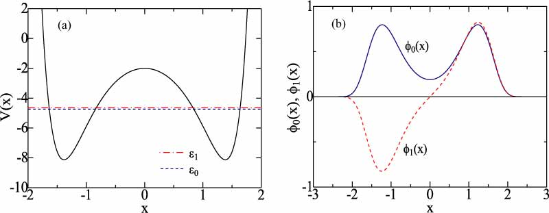
Figure 1: (Color online) (a) Razavy’s DW potential $V(x)$ (solid curve), dashed and chain curves expressing eigenvalues of $\epsilon_{0}$ and $\epsilon_{1}$, respectively, for $\hbar=m=\xi=\kappa=1.0$ [Eq.(3)]. (b) Eigenfunctions of $\phi_{0}(x)$ (solid curve) and $\phi_{1}(x)$ (dashed curve).

II.2 Eigenvalues and eigenstates of the coupled DW system

We calculate exact eigenvalues and eigenstates of the coupled two DW systems described by Eq. (2). With basis states of $\phi_{0}\phi_{0}$, $\phi_{0}\phi_{1}$, $\phi_{1}\phi_{0}$ and $\phi_{1}\phi_{1}$ where $\phi_{n}\phi_{k}\equiv\phi_{n}(x_{1})\phi_{k}(x_{2})$, the energy matrix for the Hamiltonian given by Eq. (2) is expressed by

$${\cal H} = \left({\begin{array}[]{*{20}c}{2\epsilon_{0}}&{0}&{0}&{-g\gamma^{2}}\\ {0}&{\epsilon_{0}+\epsilon_{1}}&{-g\gamma^{2}}&{0}\\ {0}&{-g\gamma^{2}}&{\epsilon_{0}+\epsilon_{1}}&{0}\\ {-g\gamma^{2}}&{0}&{0}&{2\epsilon_{1}}\\ \end{array}}\right),$$ (14)

with

$$\gamma = \int_{-\infty}^{\infty}\phi_{0}(x)\>x\>\phi_{1}(x)\>dx=1.13823.$$ (15)

Eigenvalues of the energy matrix are given by

$$E_{0} = \epsilon-\sqrt{\delta^{2}+g^{2}\gamma^{4}},$$ (16)

$$E_{1} = \epsilon-g\gamma^{2},$$ (17)

$$E_{2} = \epsilon+g\gamma^{2},$$ (18)

$$E_{3} = \epsilon+\sqrt{\delta^{2}+g^{2}\gamma^{4}},$$ (19)

where

$$\epsilon = \epsilon_{1}+\epsilon_{0}=-9.3778,$$ (20)

$$\delta = \epsilon_{1}-\epsilon_{0}=0.0863.$$ (21)

Corresponding eigenfunctions are given by

$$\Phi_{0}(x_{1},x_{2}) = \cos\theta\>\phi_{0}(x_{1})\phi_{0}(x_{2})+\sin\theta\>\phi_{1}(x_{1})\phi_{1}(x_{2}),$$ (22)

$$\Phi_{1}(x_{1},x_{2}) = \frac{1}{\sqrt{2}}\left[\phi_{0}(x_{1})\phi_{1}(x_{2})+\phi_{1}(x_{1})\phi_{0}(x_{2})\right],$$ (23)

$$\Phi_{2}(x_{1},x_{2}) = \frac{1}{\sqrt{2}}\left[-\phi_{0}(x_{1})\phi_{1}(x_{2})+\phi_{1}(x_{1})\phi_{0}(x_{2})\right],$$ (24)

$$\Phi_{3}(x_{1},x_{2}) = -\sin\theta\>\phi_{0}(x_{1})\phi_{0}(x_{2})+\cos\theta\>\phi_{1}(x_{1})\phi_{1}(x_{2}),$$ (25)

where

$$\tan\>2\theta = \frac{g\gamma^{2}}{\delta}.\;\;\;\;\mbox{$\left(-\frac{\pi}{4}\leq\theta\leq\frac{\pi}{4}\right)$}$$ (26)

Eigenvalues $E_{\nu}$ ($\nu=0-3$) are plotted as a function of $g$ in Fig. 2, which is symmetric with respect to $g=0.0$. For $g=0.0$, $E_{1}$ and $E_{2}$ are degenerate. We hereafter study the case of $g\geq 0.0$. With increasing $g$, energy gaps between $E_{0}$ and $E_{1}$ and between $E_{2}$ and $E_{3}$ are gradually decreased while that between $E_{1}$ and $E_{2}$ is increased. We note that differences between eigenvalues defined by $\Omega_{\nu}=(E_{\nu}-E_{0})/\hbar$ satisfy the relation:

$$\Omega_{3} = \Omega_{1}+\Omega_{2}.$$ (27)

For $g=0.0$, we obtain $\Omega_{1}=\Omega_{2}=\Omega_{3}/2$.

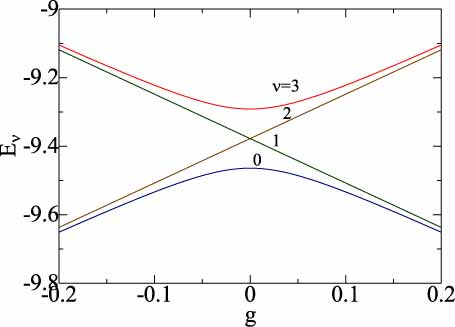
Figure 2: (Color online) Eigenvalues $E_{\nu}$ ($\nu=0-$3) of a coupled DW system as a function the coupling strength $g$.

II.3 The correlation function and orthogonality time

The time-dependent wavepacket is expressed by

$$\Psi(t) = \Psi(x_{1},x_{2},t)=\sum_{\nu=0}^{3}\>a_{\nu}\>\Phi_{\nu}(x_{1},x_{2})\>e^{-iE_{\nu}t/\hbar},$$ (28)

where expansion coefficients $a_{\nu}$ satisfy the relation

$$\sum_{\nu=0}^{3}|a_{\nu}|^{2} = 1.$$ (29)

The correlation function $\Gamma(t)$ is defined by

$$\Gamma(t) = |\int_{-\infty}^{\infty}\int_{-\infty}^{\infty}\Psi^{*}(x_{1},x_{2},0)\>\Psi(x_{1},x_{2},t)\;dx_{1}\>dx_{2}\>|,$$ (30)

$$= |\;|a_{0}|^{2}+\sum_{\nu=1}^{3}\>|a_{\nu}|^{2}\>e^{-i\Omega_{\nu}t}\>|.$$ (31)

The orthogonality time $\tau$ is provided by a time interval such that an initial wavepacket takes to evolve into the orthogonal state Giovannetti03 ; Giovannetti03b ; Batle05 ; Curilef06 ,

$$\tau = \min_{\forall\>t\>>0}\;\{\Gamma(t)=0\}.$$ (32)

In the case of wavepackets including only two states with $a_{\nu}=(1/\sqrt{2})\>(\delta_{\nu,0}+\delta_{\nu,\kappa})$, the correlation function becomes

$$\Gamma(t) = \frac{1}{2}|1+e^{-i\Omega_{\kappa}t}|=\sqrt{\frac{1+\cos\Omega_{\kappa}t}{2}},$$ (33)

for which we easily obtain $\tau$

$$\tau = \frac{\pi}{\Omega_{\kappa}}.$$ (34)

In the case of $g=0.0$, Eq. (32) becomes

$$\tau = \min_{\forall\>t}\;\large\{|a_{0}|^{2}+(|a_{1}|^{2}+|a_{2}|^{2})\>z(t)+|a_{3}|^{2}z(t)^{2}=0\large\},$$ (35)

where $z(t)=e^{-i\Omega_{1}t}$. Solutions of $\tau$ may be obtainable from roots of respective polynomial equations for $z(t)$ Batle05 ; Borras06 ; Curilef06 . In a general case, however, $\tau$ is obtainable by solving Eq. (32) with a numerical method.

II.4 The concurrence

We have calculated the concurrence of coupled DW systems. Substituting Eqs. (22)-(25) into Eq. (28), we obtain

$$|\Psi\rangle = c_{00}|0\;0\rangle+c_{01}|0\;1\rangle+c_{10}|1\;0\rangle+c_{11}|1\;1\rangle,$$ (36)

with

$$c_{00} = a_{0}\>\cos\theta\>e^{-iE_{0}t}-a_{3}\>\sin\theta\>e^{-iE_{3}t},$$ (37)

$$c_{01} = \frac{1}{\sqrt{2}}(a_{1}\>e^{-iE_{1}t}-a_{2}\>e^{-iE_{2}t}),$$ (38)

$$c_{10} = \frac{1}{\sqrt{2}}(a_{1}\>e^{-iE_{1}t}+a_{2}\>e^{-iE_{2}t}),$$ (39)

$$c_{11} = a_{0}\>\sin\theta\>e^{-iE_{0}t}+a_{3}\>\cos\theta\>e^{-iE_{3}t},$$ (40)

where $|k\;\ell\rangle=\phi_{k}(x_{1})\phi_{\ell}(x_{2})$ with $k,\ell=0,1$. The concurrence $C$ of the state $|\Psi\rangle$ given by Eq. (36) is defined by Wootters01

$$C^{2} = 4\>|c_{00}c_{11}-c_{01}c_{10}|^{2}.$$ (41)

The state given by Eq. (36) becomes factorizable if and only if the relation: $c_{00}c_{11}-c_{01}c_{10}=0$ holds. Substituting Eqs. (37)-(40) into Eq. (41), we obtain the concurrence

$$C(t)^{2} = |(a_{0}^{2}-a_{3}^{2}\>e^{-2i\Omega_{3}t})\sin 2\theta+2a_{0}a_{3}\>\cos 2\theta\>e^{-i\Omega_{3}t}-a_{1}^{2}\>e^{-2i\Omega_{1}t}+a_{2}^{2}\>e^{-2i\Omega_{2}t}|^{2},$$

whose initial value becomes

$$C(0)^{2} = |(a_{0}^{2}-a_{3}^{2})\>\sin 2\theta+2a_{0}a_{3}\>\cos 2\theta-a_{1}^{2}+a_{2}^{2}|^{2}.$$ (43)

We should note that the concurrence becomes time dependent in general for $g\neq 0.0$ because the coupling modifies the entanglement in two qubits, although it is time-independent for uncoupling case ($g=0.0$) where $\theta=0.0$ and $\Omega_{1}=\Omega_{2}=\Omega_{3}/2$.

III Model calculations and discussion

III.1 Adopted wavepackets

There are many possibilities in choosing expansion coefficients $a_{\nu}$ ($\nu=0-3$) of a wavepacket which satisfy Eq. (29). Among them, we have studied in this paper, the four wavepackets A-D whose expansion coefficients are listed in Table 1.

wavepacket	$a_{0}$	$a_{1}$	$a_{2}$	$a_{3}$
A	$\;\;\;\;\frac{1}{2}\;\;\;\;$	$\;\;\frac{1}{\sqrt{2}}\;\;$	$\;\;\;0\;\;\;$	$\;\;\;\frac{1}{2}\;\;\;$
B	$\frac{1}{\sqrt{2}}$	0	0	$\frac{1}{\sqrt{2}}$
C	$\frac{1}{\sqrt{2}}$	$\frac{1}{\sqrt{2}}$	0	0
D	$\frac{1}{2}$	$\;\;\frac{1}{2}\;\;$	$\;\;\frac{1}{2}\;\;$	$\frac{1}{2}$

Table 1 Assumed expansion coefficients $a_{\nu}$ ($\nu=0$ to 3) for four wavepackets A, B, C and D.

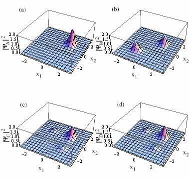
Figure 3: (Color online) Magnitudes $|\Psi(x_{1},x_{2})|^{2}$ of adopted four wavepackets of (a) A, (b) B, (c) C and (d) D for $g=0.0$ at $t=0.0$.

Coefficients in adopted wavepackets A-D are chosen as follows: A factorizable product state for $g=0.0$ is expressed by

$$\Psi_{prod} = \Psi_{R}(x_{1})\Psi_{R}(x_{2}),$$ (44)

$$= \frac{1}{2}\left[\phi_{0}(x_{1})\phi_{0}(x_{2})+\phi_{0}(x_{1})\phi_{1}(x_{2})+\phi_{1}(x_{1})\phi_{0}(x_{2})+\phi_{1}(x_{1})\phi_{1}(x_{2})\right],$$ (45)

$$= \frac{1}{2}\left[\Phi_{0}(x_{1},x_{2})+\Phi_{3}(x_{1},x_{2})\right]+\frac{1}{\sqrt{2}}\Phi_{1}(x_{1},x_{2}),$$ (46)

where magnitude of $\Psi_{R}(x_{\nu})$ $(=[\phi_{0}(x_{\nu})+\phi_{1}(x_{\nu})]/\sqrt{2})$ localizes at the right well in the $x_{\nu}$ axis ($\nu=1,\>2$). The wavepacket yielding initially the product state given by Eq. (46) is described by the wavepacket A with $a_{0}=a_{3}=1/2$ and $a_{1}=1/\sqrt{2}$.

As a typical entangled state which cannot be expressed in a factorized form, we consider the state for $g=0.0$,

$$\Psi_{ent}(x_{1},x_{2}) = \frac{1}{\sqrt{2}}\left[\phi_{0}(x_{1})\phi_{0}(x_{2})+\phi_{1}(x_{1})\phi_{1}(x_{2})\right],$$ (47)

$$= \frac{1}{\sqrt{2}}\left[\Phi_{0}(x_{1},x_{2})+\Phi_{3}(x_{1},x_{2})\right].$$ (48)

The relevant wavepacket is expressed by the wavepacket B with $a_{0}=a_{3}=1/\sqrt{2}$.

The wavepacket C consists of the ground and first-excited states with $a_{0}=a_{1}=1/\sqrt{2}$, which has been commonly adopted as a wavepacket. The wavepacket D includes four components with equal weights of $a_{\nu}=1/2$ for $\nu=0-3$.

Figures 3(a), 3(b), 3(c) and 3(d) show magnitudes $|\Psi(x_{1},x_{2})|^{2}$ of wavepackets A, B, C and D, respectively, for $g=0.0$ at $t=0.0$ generated by Eq. (28) with expansion coefficients shown in Table 1. The wavepacket A has a peak at the RR side in the $(x_{1},x_{2})$ space while the wavepacket B has two peaks at RR and LL sides, where $RR$ ($LL$) signifies the right (left) side in the $x_{1}$ axis and the right (left) side in $x_{2}$ axis. Wavepackets C and D have similar profiles with main peaks at the RR side at $t=0.0$ for $g=0.0$, but they are quite different at $t\neq 0.0$ or for $g\neq 0.0$ (compare Figs. 8 and 9 with Figs. 10 and 11, respectively). Wavepackets A, B, C and D which are initially localized in the $(x_{1},x_{2})$ space are expected to be meaningful among conceivable wavepackets.

III.2 Dynamics of $\Gamma(t)$ and $C(t)$

We will study dynamics of $\Gamma(t)$ and $C(t)$ for wavepackets A, B, C and D, which are separately described in subsections 1, 2, 3 and 4, respectively Note2 .

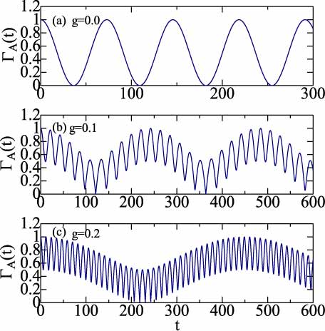
Figure 4: (Color online) Correlation function $\Gamma_{A}(t)$ for the wavepacket A with (a) $g=0.0$, (b) $g=0.1$ and (c) $g=0.2$.

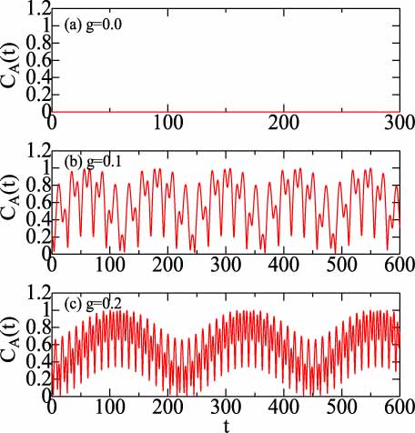
Figure 5: (Color online) Concurrence $C_{A}(t)$ for the wavepacket A with (a) $g=0.0$, (b) $g=0.1$ and (c) $g=0.2$, $C_{A}(t)$ being vanishing in (a).

III.2.1 Wavepacket A: $a_{0}=1/2$, $a_{1}=1/\sqrt{2}$, $a_{2}=0$ and $a_{3}=1/2$

From Eq. (31) and expansion coefficients in Table 1, the correlation function of the wavepacket A is given by

$$\Gamma_{A} = |\frac{1}{2}e^{-i\Omega_{1}t}+\frac{1}{4}(1+e^{-i\Omega_{3}t})|.$$ (49)

Figure 4(a) shows the correlation function $\Gamma_{A}(t)$ calculated for $g=0.0$ which yields $\tau=36.40$. Figures 4(b) and 4(c) show $\Gamma_{A}(t)$ with $g=0.1$ and $0.2$, respectively, which oscillate more rapidly than that with $g=0.0$ in Fig. 4(a). However, the orthogonality times for $g=0.1$ and 0.2 are given by $\tau=121.0$ and $218.8$, respectively, which are larger than that for $g=0.0$ (36.40).

From Eq. (LABEL:eq:K4b), the concurrence of the wavepacket A is given by

$$C_{A}(t)^{2} = \frac{1}{16}\;|2\>e^{-2i\Omega_{1}t}-2\cos 2\theta\>e^{-i\Omega_{3}t}-\sin 2\theta(1-e^{-2i\Omega_{3}t})|^{2},$$ (50)

which reduces to

$$C_{A}(0)^{2} = \frac{1}{4}\;(1-\cos 2\theta)^{2}.$$ (51)

Figure 5(a) shows that $C_{A}(t)$ for $g=0.0$ is vanishing independently of time. We note in Figs. 5(b) and 5(c) that when the coupling is introduced, $C_{A}(t)$ with initial values of $C_{A}(0)=0.223$ and 0.342 for $g=0.1$ and $0.2$, respectively, show complex time dependence which arises from a superposition of multiple contributions with frequencies of $\Omega_{1}$, $\Omega_{3}$, $\Omega_{3}-\Omega_{1}$ and $\Omega_{3}-2\Omega_{1}$.

The temporal average of $\langle C_{A}(t)^{2}\rangle$ may be analytically calculated as

$$C_{av}^{2}=\langle C_{A}(t)^{2}\rangle = \frac{1}{8}(4-\sin^{2}2\theta)\hskip 28.45274pt\mbox{for $g>0.0$},$$ (52)

$$= 0\hskip 85.35826pt\mbox{for $g=0.0$}.$$

Note that $C^{2}_{av}$ has the discontinuity at $g=0.0$ where $\Omega_{3}-2\Omega_{1}=0$ (Fig. 2) Note1 . We obtain $C_{av}=0.0$, 0.707, 0.643 and 0.622 for $g=0$, $0_{+}$, 0.1 and 0.2, respectively, where $0_{+}=\lim_{\epsilon\rightarrow 0}0+\epsilon$.

III.2.2 Wavepacket B: $a_{0}=1/\sqrt{2}$, $a_{1}=a_{2}=0.0$ and $a_{3}=1/\sqrt{2}$

The correlation function of the wavepacket B is given by

$$\Gamma_{B}(t) = \frac{1}{2}(1+e^{-i\Omega_{3}t}),$$ (53)

which leads to $\tau=\pi/\Omega_{3}$. Figures 6(a), 6(b) and 6(c) show $\Gamma_{B}(t)$ for $g=0.0$, 0.1 and 0.2, respectively, for which the orthogonality times are $\tau=18.2$, 10.1 and 5.75.

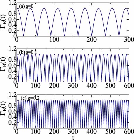
Figure 6: (Color online) Correlation function $\Gamma_{B}(t)$ for the wavepacket B with (a) $g=0.0$, (b) $g=0.1$ and (c) $g=0.2$.

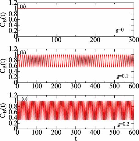
Figure 7: (Color online) Concurrence $C_{B}(t)$ for the wavepacket B with (a) $g=0.0$, (b) $g=0.1$ and (c) $g=0.2$.

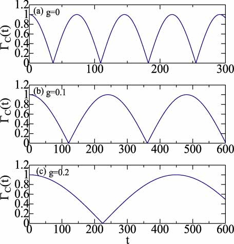
Figure 8: (Color online) Correlation function $\Gamma_{C}(t)$ for the wavepacket C with (a) $g=0.0$, (b) $g=0.1$ and (c) $g=0.2$.

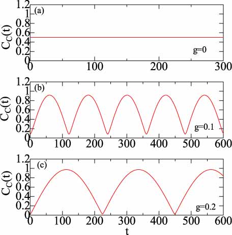
Figure 9: (Color online) Concurrence $C_{C}(t)$ for the wavepacket C with (a) $g=0.0$, (b) $g=0.1$ and (c) $g=0.2$.

The concurrence of the wavepacket B is expressed by

$$C_{B}(t)^{2} = \frac{1}{4}|\sin 2\theta(1-e^{-2i\Omega_{3}t})+2\cos 2\theta\>e^{-i\Omega_{3}t}|^{2},$$ (54)

with

$$C_{B}(0)^{2} = \cos^{2}2\theta,$$ (55)

from which we obtain $C_{B}(0)=1.0$, 0.554 and 0.316 for $g=0.0$, 0.1 and 0.2, respectively. Calculated $C_{B}(t)$ for $g=0.0$, 0.1 and 0.2 are plotted in Figs. 7(a), 7(b) and 7(c), respectively. $C_{B}(t)$ for $g=0.0$ is unity independently of time. When the coupling $g$ is introduced, $C_{B}(t)$ becomes time dependent, showing rapid oscillations as shown in Figs. 7(b) and 7(c).

The temporal average of $\langle C_{B}(t)^{2}\rangle$ is given by

$$C_{av}^{2} = \langle C_{B}(t)^{2}\rangle=1-\frac{1}{2}\sin^{2}2\theta,$$ (56)

which leads to $C_{av}=1.0$, 0.808 and 0.742 for $g=0.0$, 0.1 and 0.2, respectively.

III.2.3 Wavepacket C: $a_{0}=a_{1}=1/\sqrt{2}$ and $a_{2}=a_{3}=0.0$

The correlation function of the wavepacket C is given by

$$\Gamma_{C}(t) = \frac{1}{2}(1+e^{-i\Omega_{1}t}),$$ (57)

leading to $\tau=\pi/\Omega_{1}$. Figures 8(a), 8(b) and 8(c) show $\Gamma_{C}(t)$ for $g=0.0$, 0.1 and 0.2, respectively, from which the orthogonality time is given by $\tau=36.40$, 120.3 and 224.5.

The concurrence of the wavepacket C is expressed by

$$C_{C}(t)^{2} = \frac{1}{4}\;|e^{-2i\Omega_{1}t}-\sin{2\theta}|^{2},$$ (58)

which reduces to

$$C_{C}(0)^{2} = \frac{1}{4}(1-\sin 2\theta)^{2}.$$ (59)

We obtain $C_{C}(0)=0.5$, 0.0839 and 0.0256 for $g=0.0$, 0.1 and 0.2, respectively. Figure 9(a) shows the time-independent $C_{C}(t)=0.5$ for $g=0.0$. For $g=0.1$ and $0.2$, $C_{C}(t)$ show oscillations as shown in Figs. 9(b) and 9(b).

The temporal average is given by

$$C_{av}^{2} = \langle C_{C}(t)^{2}=\frac{1}{4}(1+\sin^{2}2\theta),$$ (60)

which yields $C_{av}=0.5$, 0.651 and 0.689 for $g=0.0$, 0.1 and 0.2, respectively.

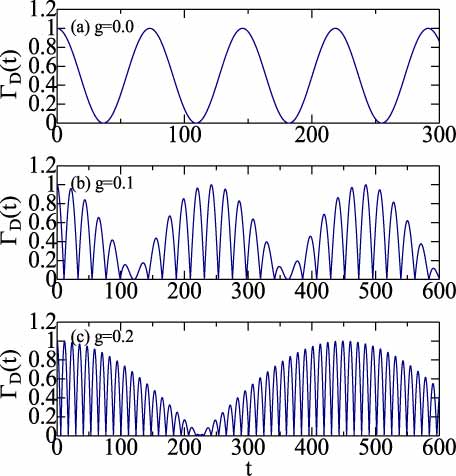
Figure 10: (Color online) Correlation function $\Gamma_{D}(t)$ for the wavepacket D with (a) $g=0.0$, (b) $g=0.1$ and (c) $g=0.2$.

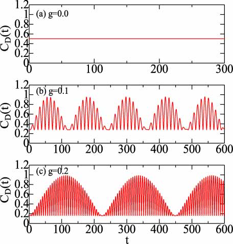
Figure 11: (Color online) Concurrence $C_{D}(t)$ for the wavepacket D with (a) $g=0.0$, (b) $g=0.1$ and (c) $g=0.2$.

III.2.4 Wavepacket D: $a_{0}=a_{1}=a_{2}=a_{3}=1/2$

The correlation function of the wavepacket D is expressed by

$$\Gamma_{D}(t) = \frac{1}{4}|1+e^{-i\Omega_{1}t}+e^{-i\Omega_{2}t}+e^{-i\Omega_{3}t}|,$$ (61)

$$= \frac{1}{4}|(1+e^{-i\Omega_{1}t})(1+e^{-i\Omega_{2}t})|,$$ (62)

where Eq. (27) is employed. For $g=0.0$, $\Gamma_{D}(t)$ shows a simple sinusoidal oscillation because $\Omega_{1}=\Omega_{2}=\Omega_{3}/2$ [Fig. 10(a)]. For $g\neq 0.0$, however, $\Gamma_{D}(t)$ exhibits a rather complex oscillation as shown in Figs. 10(b) and 10(c), where $\Gamma_{D}(t)$ vanishes at $t=36.40\>(2k+1)$, $11.02\>(2k+1)$ and $5.903\>(2k+1)$ for $g=0.0$, 0.1 and 0.2, respectively, with $k=0,1,2\cdots$. We obtain the orthogonality time expressed by $\tau=\pi/\Omega_{2}$, which leads to $\tau=36.40$, 11.02 and 5.903 for $g=0.0$, 0.1 and 0.2, respectively.

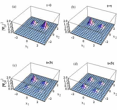
Figure 12: (Color online) Magnitudes of $|\Psi_{D}(x_{1},x_{2},t)|^{2}$ of the wavepacket D with $g=0.1$ at (a) $t=0$, (b) $t=\tau$, (c) $t=3\tau$ and (d) $t=5\tau$, $\Psi_{D}(x_{1},x_{2},t)$ at $t=\tau$, $3\tau$ and $5\tau$ being orthogonal to $\Psi_{D}(x_{1},x_{2},0)$.

The concurrence of the wavepacket D is given by

$$C_{D}(t)^{2} = \frac{1}{16}\;|\sin 2\theta(1-e^{-2i\Omega_{3}t})+2\cos{2\theta}\>e^{-i\Omega_{3}t}-e^{-2i\Omega_{1}t}+e^{-2i\Omega_{2}t}|^{2},$$ (63)

with

$$C_{D}(0)^{2} = \frac{1}{4}\cos^{2}2\theta,$$ (64)

yielding $C_{D}(0)=0.5$, 0.277 and 0.158 for $g=0.0$, 0.1 and 0.2, respectively. Although $C_{D}(t)$ for $g=0.0$ is 0.5 independently of $t$ in Fig. 11(a), $C_{D}(t)$ for $g=0.1$ and 0.2 show complicated time dependence in Figs. 11(b) and 11(c), respectively.

The averaged concurrence is given by

$$C_{av}^{2}=\langle C_{D}(t)^{2}\rangle = \frac{1}{8}(3-\sin^{2}2\theta)\hskip 28.45274pt\mbox{for $g>0.0$},$$ (65)

$$= \frac{1}{4}\hskip 85.35826pt\mbox{for $g=0.0$},$$ (66)

where a discontinuity arises from the relation: $\Omega_{1}-\Omega_{2}\rightarrow 0$ as $g\rightarrow 0.0$ Note1 . We obtain $C_{av}=0.5$, 0.612, 0.537 and 0.512 for $g=0$, $0_{+}$, 0.1 and 0.2, respectively.

Before closing the subsection of Sec. III B, it is worthwhile to make a closer look to the dynamical properties of wavefunctions. There is one kind of wavepackets which is orthogonal to the initial wavepacket A, B or C: for example, $|\Psi_{A}(x_{1},x_{2},\tau(2k+1))|^{2}$ with $k=0,1,2,\cdots$ has a peak at the LL side while $|\Psi_{A}(x_{1},x_{2},0)|^{2}$ at the RR side. It is, however, not the case for the wavepacket D. Magnitudes of wavefunctions $|\Psi_{D}(x_{1},x_{2},t)|^{2}$ for $g=0.1$ at $t=0.0$, $\tau$, $3\tau$ and $5\tau$ ($\tau=11.02$) are plotted in Figs. 12(a)-12(d), respectively, where all wavefunctions in Figs. 12(b), 12(c) and 12(d) are orthogonal to that in Fig. 12(a).

III.3 The $g$ dependence of $\tau$ and $\tau_{min}$

Although calculations in the preceding subsection Sec. III B have been reported only for $g=0.0$, 0.1 and 0.2, we may repeat calculations of the orthogonality time $\tau$ by changing $g$ for the four wavepackets. Calculated $\tau$ is plotted as a function of $g$ by dashed curves in Figs. 13(a)-13(d). Obtained $\tau$ for the four wavepackets is expressed in the second column of Table 2, whose third and fourth columns show $C^{2}_{av}$ and $C(0)^{2}$, respectively, $E_{\nu}$ ($\nu=0-3$) and $\theta$ being $g$ dependent [Eqs. (16)-(19), (26)]. Figures 13(a)-13(d) show that with increasing $g$, $\tau_{A}$ and $\tau_{C}$ are increased, while $\tau_{B}$ and $\tau_{D}$ are decreased. This is because with increasing $g$, a gap of $E_{1}-E_{0}$ is decreased whereas $E_{3}-E_{0}$ and $E_{2}-E_{0}$ are increased (Fig. 2).

wavepacket	$\;\;\;\tau\;\;\;$	$C^{2}_{av}$	$C(0)^{2}$
A	$\;\;\;\;\simeq\frac{\pi\hbar}{(E_{1}-E_{0})}\;\;\;\;$	$\;\;\frac{1}{8}(4-\sin^{2}2\theta)-\frac{1}{2}\>\delta(g)\;\;$	$\;\;\;\frac{1}{4}(1-\cos 2\theta)^{2}\;\;\;$
B	$\frac{\pi\hbar}{(E_{3}-E_{0})}$	$1-\frac{1}{2}\sin^{2}2\theta$	$\cos^{2}2\theta$
C	$\;\;\;\frac{\pi\hbar}{(E_{1}-E_{0})}\;\;\;$	$\frac{1}{4}(1+\sin^{2}2\theta)$	$\frac{1}{4}(1-\sin 2\theta)^{2}$
D	$\frac{\pi\hbar}{(E_{2}-E_{0})}$	$\frac{1}{8}(3-\sin^{2}2\theta)-\frac{1}{8}\>\delta(g)$	$\frac{1}{4}\cos^{2}2\theta$

Table 2 Calculated $\tau$, $C^{2}_{av}$ and $C(0)^{2}$ for four wavepackets A, B, C and D.

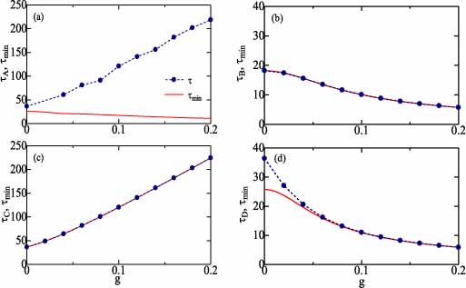
Figure 13: (Color online) The $g$ dependence of the orthogonality time $\tau$ (dashed curves) and minimum values $\tau_{min}$ (solid curves) for (a) wavepacket A, (b) B, (c) C and (d) D.

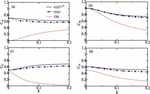
Figure 14: (Color online) The $g$ dependence of averaged concurrences, $C_{av}$ [$=\sqrt{\langle C(t)^{2}\rangle}$] (solid curves) and $\langle C(t)\rangle$ (chain curves), and of the initial concurrence $C(0)$ (dashed curves) for (a) wavepacket A, (b) B, (c) C and (d) D.

We may evaluate the minimum orthogonality time $\tau_{min}$ of our DW model, calculating the expectation energy $E$ and its root-mean-square value $\Delta E$ in Eq. (1), which are expressed by

$$E = \sum_{\nu}\>|a_{\nu}|^{2}\>(E_{\nu}-E_{0})=|a_{1}|^{2}\Omega_{1}+|a_{2}|^{2}\Omega_{2}+|a_{3}|^{2}\Omega_{3},$$ (67)

$$(\Delta E)^{2} = \sum_{\nu}\>|a_{\nu}|^{2}\>(E_{\nu}-E_{0})^{2}-E^{2}=|a_{1}|^{2}\Omega_{1}^{2}+|a_{2}|^{2}\Omega_{2}^{2}+|a_{3}|^{2}\Omega_{3}^{2}-E^{2}.$$ (68)

Solid curves in Figs. 13(a)-13(d) express $\tau_{min}$ calculated by Eqs. (1), (67) and (68) as a function of $g$ for four wavepackets A-D. With increasing $g$, $\tau_{min}$ increases for the wavepacket C, whereas those for wavepackets A, B and D decrease. The ratio of $\tau/\tau_{min}$ is unity for wavepackets B and C in Figs. 13(b) and 13(c). However, we obtain $\tau/\tau_{min}=1.414$ and 1.0 for $g=0.0$ and $g\gtrsim 0.06$, respectively, for the wavepacket D in Fig. 13(d). Furthermore, this ratio more apparently exceeds unity for the wavepacket A in Fig. 13(a) where $\tau/\tau_{min}$ $=1.414$, 7.00 and 20.0 for $g=0.0$, 0.1 and 0.2, respectively. This is accounted for by the fact that with increasing $g$, $\tau$ is increased because of a narrowed energy gap of $E_{1}-E_{0}$ while $\tau_{min}$ is decreased by a high-energy contribution of $E_{3}-E_{0}$ to $E$ (Fig. 2) .

III.4 $g$ dependence of $C_{av}$ and $C(0)$

We may calculate $C_{av}$ and $C(0)$ of the four wavepackets as a function of $g$, whose results are plotted in Figs. 14(a)-14(d). In the wavepacket A, $C_{av}$ has a discontinuity at $g=0.0$ as mentioned before: $C_{av}=0.0$ and 0.707 at $g=0$ and $0_{+}$, respectively. When $g$ is introduced, $C(0)$ is increased from zero while $C_{av}$ is decreased from $0.707$ [Fig. 14(a)]. In the wavepacket B, both $C_{av}$ and $C(0)$ are gradually decreased with increasing $g$ [Fig. 14(b)]. On the contrary, in the wavepacket C, $C_{av}$ is increased from 0.5 but $C(0)$ is decreased form 0.5 when $g$ is introduced [Fig. 14(c)]. In the wavepacket D, $C_{av}$ has a discontinuity at $g=0.0$: $C_{av}=0.5$ and 0.612 at $g=0$ and $0_{+}$, respectively, and both $C_{av}$ and $C(0)$ are decreased with increasing $g$ [Fig. 14(d)].

Chain curves in Figs. 14(a)-14(d) show $\langle C(t)\rangle$ for the four wavepackets, which are nearly in agreement with $C_{av}$ ($=\sqrt{C(t)^{2}}$) plotted by solid curves.

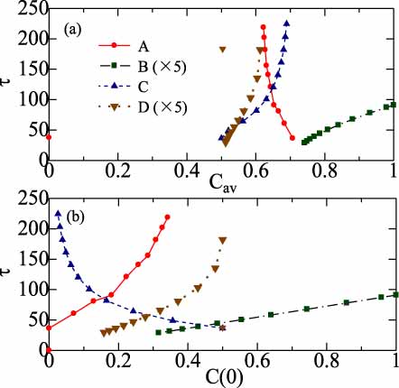
Figure 15: (Color online) (a) $C_{av}$ vs. $\tau$ and (b) $C(0)$ vs. $\tau$ for wavepackets A (circles), B (squares), C (triangles) and D (inverted triangles), $\tau$ for wavepackets B and D being multiplied by a factor of five. In (a), a point at $(C_{av},\tau)=(0.0,36.40)$ for the wavepacket A is separated from that at $(0.706,36.40)$ because of the discontinuity of $C_{av}$ at $g=0.0$ (Fig. 14). Similarly, a point at $(C_{av},\tau)=(0.5,36.40)$ for the wavepacket D is separated from that at $(0.6124,36.40)$.

III.5 The dependence of $\tau$ on $C_{av}$ and $C(0)$

Comparing Figs. 13(a)-13(d) and Figs. 14(a)-14(d), respectively, we may examine the relation between the orthogonality time ($\tau$) and the concurrence ($C_{av}$ or $C(0)$). Figures 15(a) and 15(b) show the $C_{av}$ vs. $\tau$ plot and the $C(0)$ vs. $\tau$ plot, respectively. For wavepackets B and D (squares and inverted triangles), $\tau$ is increased with increasing $C_{av}$ or $C(0)$. We note, however, that $\tau$ of the wavepacket A (circles) is increased with increasing $C(0)$ but with decreasing $C_{av}$. On the contrary, $\tau$ of the wavepacket C (triangles) is increased with increasing $C_{av}$ but with decreasing $C(0)$. Figures 15(a) and 15(b) imply that the effect of $C_{av}$ on $\tau$ is generally different from that of $C(0)$ and that when the concurrence is increased, the orthogonality time may be increased or decreased, depending on the adopted wavepacket. This is in contrast with Refs. Giovannetti03 ; Batle05 ; Curilef06 but in agreement with Refs. Giovannetti03b ; Borras06 ; Zander13 .

IV Concluding remark

Batle et al. Batle05 and Curilef et al. Curilef06 studied two uncoupled qubits with eigenvalues

$$E_{0}=0,\;\;\;E_{1}=E_{2}=\epsilon_{1},\;\;\;E_{3}=2\epsilon_{1},$$ (69)

where $\epsilon_{1}$ stands for an energy of a free qubit. For wavepackets with $|a_{0}|^{2}=|a_{3}|^{3}\neq 0.0$, the ratio of $\tau/\tau_{min}$ is shown to be unity for a maximally entangled state and $\sqrt{2}$ for a separate state Batle05 ; Curilef06 . In our wavepackets A, B and D with $a_{3}=a_{0}\neq 0.0$ for $g=0.0$, the ratio is $\tau/\tau_{min}=1.0$ in the wavepacket B while it is $\sqrt{2}$ in wavepackets A and D, which are consistent with results of Refs. Batle05 ; Curilef06 . However, in the wavepacket C with $a_{3}=0.0$, which corresponds to the singular case after Chau Chau10 , we obtain $\tau/\tau_{min}=1.0$ for $g=0.0$ although it is not a maximally entangled state ($C=0.5$), in agreement with Ref. Chau10 .

Zander et al. Zander13 adopted two interacting qubits given by the Hamiltonian

$$H = \hbar\omega_{0}[2I^{(1)}\otimes I^{(2)}-\sigma_{x}^{(1)}\otimes I^{(2)}-I^{(1)}\otimes\sigma_{x}^{(2)}]+\hbar\omega[I^{(1)}\otimes I^{(2)}-\sigma_{x}^{(1)}\otimes\sigma_{x}^{(2)}],$$ (70)

where $\omega_{0}$ expresses the energy of free qubits, $\omega$ stands for the interaction, $I$ is the identity matrix and $\sigma_{x}$ is the $x$-Pauli matrix. Eigenvalues of the Hamiltonian are Zander13

$$E_{0}=0,\;\;\;E_{1}=E_{2}=2\hbar(\omega+\omega_{0}),\;\;\;E_{3}=4\hbar\omega_{0}.$$ (71)

Ref. Zander13 studied effects of entanglement on the evolution speed in interacting two qubits, evaluating the linear entropy mainly for the three cases of $\omega=\omega_{0}$, $\omega_{0}=0$ and $\omega=3\omega_{0}$ with arbitrary expansion coefficients $\{a_{\nu}\}$ for wavepackets. The study of Ref. Zander13 is complementary to ours in which calculations have been made for an arbitrary interaction $g$ with four sets of expansion coefficients $\{a_{\nu}\}$ for wavepackets A-D. It was claimed in Ref. Zander13 that with the exception of some special cases, states with a small initial entanglement tend to evolve in the fastest way in coupled qubits. This is not inconsistent with our result of the wavepacket A showing that $\tau/\tau_{min}=7.00$ and $20.0$ for $C(0)=0.223$ and 0.342, respectively. However, we obtain $\tau/\tau_{min}=1.0$ almost independently of $C(0)$ in wavepackets B, C, and D (Figs. 13 and 14), which might correspond to special cases after Ref. Zander13 . Refs. Giovannetti03 and Zander13 explained that for $\tau$ to reach the bound, it is necessary to have either an initial entangled state, or an interaction term capable of creating entanglement. This seems not to be applicable to the wavepacket A for which $\tau/\tau_{min}=20.0\gg 1.0$ even if $C(0)=0.342$ for $g=0.2$ (Figs. 13 and 14). This disagreement might arise from a difference in models adopted in Ref. Zander13 and the present study: the interaction dependence of eigenvalues in Eq. (71) are different from that in Eqs. (16)-(19).

In the simple case, we may obtain an analytical expression for $\tau$ expressed in terms of $C_{av}$ and/or $C(0)$. Indeed, for the wavepacket B, a calculation with Eqs. (26), (55)and (56) leads to

$$\tau_{B} = \tau_{min}=\left(\frac{\pi}{2\delta}\right)\>\sqrt{2C_{av}^{2}-1}=\left(\frac{\pi}{2\delta}\right)C(0),$$ (72)

which is numerically confirmed in Fig. 15. Unfortunately it is impossible to obtain analytical results for wavepackets A, C and D.

In summary, we have studied dynamical properties of four wavepackets A, B, C and D (Table 1), by using an exactly solvable coupled DW system described by Razavy’s potential Razavy80 . Our model calculations yield the followings:

(1) The correlation function $\Gamma(t)$ and concurrence $C(t)$ in interacting two qubits show complicate and peculiar time dependence (Figs. 4-11),

(2) The quantum evolution speed measured by $\tau^{-1}$ is not necessarily increased by an introduced interaction $g$: e.g. it is decreased in wavepackets A and C (Fig. 13),

(3) The concurrence, $C_{av}$ or $C(0)$, may be decreased by an increased interaction (Fig. 14),

(4) The relation between $C(0)$ and $\tau$ is generally not the same as that between $C_{av}$ and $\tau$, and the evolution speed may be increased or decreased with the increased concurrence ($C_{av}$ or $C(0)$), depending on a wavepacket (Fig. 15), and

(5) $\tau$ may not reach its minimum value $\tau_{min}$ even when the entanglement is present in coupled DW systems.

Items (4) and (5) are in contrast with the non-interacting case where $\tau$ is decreased with increasing $C(0)$ and the ratio $\tau/\tau_{min}$ approaches unity in entangled state Giovannetti03 ; Giovannetti03b ; Batle05 ; Borras06 ; Curilef06 . Items (4) and (5) suggest that the relation between the evolution speed and the entanglement in coupled qubits is not definite in contrast to that in uncoupled case Giovannetti03 ; Giovannetti03b ; Batle05 ; Borras06 ; Curilef06 . In the present study, we do not take into account environmental effects which are expected to play important roles in real DW systems. An inclusion of dissipative effects is left as our future subject.

- (1) M. J. Storcz and F. K. Wilhelm, Phys. Rev. A 67 (2003) 042319.
- (2) N. Margolus and L. B. Levitin, Physica D 120 (1998) 188.
- (3) L. Mandelstam and I. G. Tamm, J. Phys. USSR 9 (1945) 249; K. Bhattacharyya, J. Phys. A 16 (1983) 2993; P. Pfeifer, Phys. Rev. Lett. 70 (1993) 3365.
- (4) V. Giovannetti, S. Lloyd, and L. Maccone, Europhys. Lett. 62 (2003) 615.
- (5) V. Giovannetti, S. Lloyd, and L. Maccone, Phys. Rev. A 67 (2003) 052109.
- (6) J. Batle, M. Casas, A. Plastino, and A. R. Plastino, Phys. Rev. A 72 (2005) 032337.
- (7) S. Curilef, C. Zander and A. R. Plastino, Eur. J. Phys. 27 (2006) 1193.
- (8) A. Borrás, M. Casas, A. R. Plastino, and A. Plastino, Phys. Rev. A 74 (2006) 022326.
- (9) H. F. Chau, Phys. Rev. A 82 (2010) 056301.
- (10) C. Zander, A. Borras, A. R. Plastino, A. Plastino, and M. Casas, J. Phys. A 46, 095302 (2013).
- (11) D. J. Tannor, Introduction to quantum mechanics: A time-dependent perspective (Univ. Sci. Books, Sausalito, California, 2007).
- (12) M. Razavy, Am. J. Phys. 48 (1980) 285.
- (13) F. Finkel, F. Finkel, A. Gonzalez-Lopez and M. A. Rodriguez, J. Phys. A 32 (1999) 6821.
- (14) B. Bagchi and A. Ganguly, J. Phys. A 36 (2003) L161.
- (15) The energy and time are measured in units of and , respectively, in this study.
- (16) W. K. Wootters, Quan. Inf. Comp. 1 (2001) 27.
- (17) In the wavepacket A, one term in leads to which yields the delta-function contribution at where . The situation is similar to the wavepacket D in which at .