The Higgs oscillator on the hyperbolic plane and Light Front Holography

Abstract

The Light Front Holographic (LFH) wave equation, which is the conformal scalar equation on the plane, is revisited from the perspective of the supersymmetric quantum mechanics, and attention is drawn to the fact that it naturally emerges in the small hyperbolic angle approximation to the “curved” Higgs oscillator on the hyperbolic plane, i.e. on the upper part of the two-dimensional hyperboloid of two sheets, H${}_{+R}^{2}$, a space of constant negative curvature. Such occurs because the particle dynamics under consideration reduces to the one dimensional Schrödinger equation with the second hyperbolic Pöschl-Teller potential, whose flat-space (small-angle) limit reduces to the conformally invariant inverse square distance plus harmonic oscillator interaction, on which LFH is based. In consequence, energies and wave functions of the LFH spectrum can be approached by the solutions of the Higgs oscillator on the hyperbolic plane in employing its curvature and the potential strength as fitting parameters. Also the proton electric charge form factor is well reproduced within this scheme by means of a Fourier-Helgason hyperbolic wave transform of the charge density. In conclusion, in the small angle approximation, the Higgs oscillator on H${}_{+R}^{2}$ is demonstrated to satisfactory parallel essential outcomes of the Light Front Holographic QCD. The findings are suggestive of associating the H${}_{+R}^{2}$ curvature with a second scale in LFH, which then could be employed in the definition of a chemical potential.

I Introduction to the LFH wave equation. Goals and motivation.

Supersymmetric quantum mechanics has exercised over the years notable influence on various fields of spectroscopic studies by providing an efficient machinery in handling a large variety of interactions in complex systems by means of exactly solvable potentials CooperKhare . Specifically in particle physics, one repeatedly faces situations in which most complicated field-theoretical considerations amount to known Sturm-Liouville problems, a prominent example being the Light-Front Holographic QCD Review –BdTD . This approach is derived from the first-principle motivated gauge-gravity duality concept and is quite successful in describing a broad range of hadron properties. At its root one finds two effective one-dimensional Schrödinger equations with an inverse square distance plus harmonic oscillator potential, which defines the conformal scalar equations on the plane according to,

$$\left(-\frac{{\mathrm{d}}^{2}}{{\mathrm{d}}\zeta^{2}}+\frac{\nu^{2}-\frac{1}{4}}{\zeta^{2}}+\kappa^{4}\zeta^{2}+c_{+}^{\nu}\right)\Psi^{n\nu}_{+}(\zeta)=E^{2}\Psi^{n\nu}_{+}(\zeta),\,\,c^{\nu}_{+}=2\kappa^{2}(\nu+1),$$ (1)

$$\left(-\frac{{\mathrm{d}}^{2}}{{\mathrm{d}}\zeta^{2}}+\frac{(\nu+1)^{2}-\frac{1}{4}}{\zeta^{2}}+\kappa^{4}\zeta^{2}+c_{-}^{\nu}\right)\Psi^{n(\nu+1)}_{-}(\zeta)=E^{2}\Psi^{n(\nu+1)}_{-}(\zeta),\,\,c_{-}^{\nu}=2\kappa^{2}\nu,$$ (2)

with $1/\kappa$ being an external lengths scale. The equations (1)-(2) can be viewed either as one-dimensional Klein-Gordon equations, or equivalently, as one-dimensional Schrödinger equations under the identifications,

$$E^{2}=\frac{2\mu c^{2}E^{Schr}}{\hbar^{2}c^{2}},\quad\kappa^{4}=\frac{\mu^{2}\omega^{2}}{\hbar^{2}},\quad\left[E^{2}\right]={\mbox{fm}}^{-2},\quad E^{2}={\mathcal{M}}^{2},$$ (3)

where $E^{Schr}$ is the energy in MeV of a particle of mass $\mu$ in the stationary Schrödinger equation or, the reduced mass of a two-body system, such as quark–diquark (q-qq), with $\zeta$ being associated with a relative distance. In introducing the operators, $B^{+}_{\nu}$ and $B_{\nu}$, laddering back and forth between $\Psi_{-}^{n(\nu+1)}(\zeta)$ and $\Psi_{+}^{n\nu}(\zeta)$ according to,

$$B^{+}_{\nu}\Psi_{-}^{n(\nu+1)}(\zeta) = E\Psi_{+}^{n\nu}(\zeta),\quad B^{+}_{\nu}=-\frac{{\mathrm{d}}}{{\mathrm{d}}\zeta}-\frac{\nu+\frac{1}{2}}{\zeta}-\kappa^{2}\zeta,$$

$$B_{\nu}\Psi_{+}^{n\nu}(\zeta) = E\Psi_{-}^{n(\nu+1)}(\zeta),\quad B_{\nu}=\frac{{\mathrm{d}}}{{\mathrm{d}}\zeta}-\frac{\nu+\frac{1}{2}}{\zeta}-\kappa^{2}\zeta,\quad$$ (4)

one finds a Dirac-like factorization of the equations (1) and (2),

$$B^{+}_{\nu}B_{\nu}\Psi_{+}^{n\nu}=E^{2}\Psi_{+}^{n\nu}, B_{\nu}B^{+}_{\nu}\Psi_{-}^{n(\nu+1)}=E^{2}\Psi_{-}^{n(\nu+1)},$$ (5)

admittedly with vectorial rather than scalar inverse-distance plus linear potentials. The explicit solutions to (1) and (2) read,

$$\Psi^{n\nu}_{+}(\zeta) = N_{n\nu}(\kappa^{2}\zeta^{2})^{\frac{\nu}{2}+\frac{1}{4}}e^{-\frac{\kappa^{2}\zeta^{2}}{2}}L_{n}^{\nu}(\kappa^{2}\zeta^{2}),\,L_{n}^{\nu}(\kappa^{2}\zeta^{2})\sim\,_{1}F_{1}(-n,\nu+1,\kappa^{2}\zeta^{2}),$$

$$\Psi^{n(\nu+1)}_{-}(\zeta) = {\bar{N}}_{n\nu}(\kappa^{2}\zeta^{2})^{\frac{\nu+1}{2}+\frac{1}{4}}e^{-\frac{\kappa^{2}\zeta^{2}}{2}}L_{n}^{\nu+1}(\kappa^{2}\zeta^{2}),\,E^{2}=4\hbar^{2}c^{2}\kappa^{2}\left(n+\nu+1\right)$$ (6)

$$= 4\hbar^{2}c^{2}\kappa^{2}\left(n+\frac{\nu+1}{2}\right)+c^{\nu}_{+}=4\hbar^{2}c^{2}\kappa^{2}\left(n+\frac{\nu+2}{2}\right)+c^{\nu}_{-},$$

with $c^{\nu}_{+}$ from (1) and $c_{-}^{\nu}$ from (2). Here $L_{n}^{\nu}$ are the generalized Laguerre polynomials, $N_{n\nu}$, and ${\bar{N}}_{n\nu}$ are normalization constants, and ${}_{1}F_{1}$ stands for the confluent hypergeometric function. In being distinct by $\Delta\nu=1$, $\Psi^{n\nu}_{+}(\zeta)$, and $\Psi^{n(\nu+1)}_{-}(\zeta)$ are given within the LFH method under discussion the interpretation of a large and a small component of a Dirac spinor, thus allowing to correct for the scalar nature of eqs. (1)–(2).

The first goal of the present study is to comment on some specific supersymmetric quantum mechanical aspects of the above equations (1) and (2) and explore consequences. The pair of wave functions, $\Psi^{n\nu}_{+}(\zeta)$, and $\Psi_{-}^{n(\nu+1)}(\zeta)$, in reality describe states belonging to either even or odd principal quantum numbers, $N_{+}=(2n+\nu)$, and $N_{-}=(2n+\nu+1)$, of the three dimensional harmonic oscillator, distinct by one unit. In addition, they belong to a pair of supersymmetric partner spectra, and the corresponding SUSY-QM equations satisfied by them predict distinct energy excitations, $E_{+}=4\hbar^{2}c^{2}\kappa^{2}n$, versus $E_{-}=4\hbar^{2}\kappa^{2}(n+1)$, respectively. This energy separation has been removed in the above LFH equations (1) and (2) through shifts of the respective SUSY-QM Hamiltonians by the additive constants $2c_{+}^{\nu}$, and $2c_{-}^{\nu}$, respectively. Gaining a deeper insight into the nature of the $\Psi^{n\nu}$–$\Psi^{n(\nu+1)}$ wave functions would allow to understand as two what extent the consideration of such pairs as Dirac spinor components is amenable to generalizations to other potentials.

The next goal of the present study is to show that  (1)-(2) represent the decreasing curvature limit of quantum motion on the hyperbolic plane within the Higgs oscillator potential and to explore consequences. The paper is structured as follows. The next section is devoted to the SUSY-QM aspects of the equations (1)-(2). In section 3 we briefly highlight the basics of quantum motion on the hyperbolic plane, define the Higgs oscillator potential problem there, and show that it is equivalent to the one dimensional Schrödinger equation with the generalized hyperbolic Pöschl-Teller potential CooperKhare . In section 4 we take the small hyperbolic angle limit of the latter equation and its solutions and reveal their equivalence to the LFH wave equation and its solutions. We furthermore calculate the proton electric charge form factor and draw conclusions on the relevance of the conformal symmetry in the two extreme regimes of QCD, the infrared and the ultraviolet. The paper closes with brief conclusions and has one Appendix.

II The SUSY-QM aspects of Light-Front Holography and conformal symmetry

We first notice that, modulo the additive constants, $c_{\nu}^{+}$, and $c_{\nu}^{-}$, the equations (1), (2) are known from the SuperSymmetric Quantum Mechanics (SUSY-QM) of the three dimesnional (3D) harmonic oscillator in the presence of a centrifugal barrier CooperKhare . In using $\hbar=1$, $2\mu=1$ units, and introducing the operators $A_{\nu}$ and $A^{+}_{\nu}$, as

$$A^{+}_{\nu}=-\frac{{\mathrm{d}}}{{\mathrm{d}}\zeta}+{\mathcal{W}}_{\nu}(\zeta), A_{\nu}=\frac{{\mathrm{d}}}{{\mathrm{d}}\zeta}+{\mathcal{W}}_{\nu}(\zeta),\quad{\mathcal{W}}_{\nu}(\zeta)=-\frac{\nu+\frac{1}{2}}{\zeta}+\kappa^{2}\zeta,$$ (7)

where ${\mathcal{W}}_{\nu}(\zeta)$ is the superpotential, it is straightforward to calculate that the $n=0$ function, $\Psi^{01}_{+}(\zeta)$ in (6) is nullified by $A_{1}$,

$$A_{1}\Psi^{01}_{+}(\zeta)=0,$$ (8)

meaning that it refers to a genuine SUSY-QM ground state. This ground state is vanishing in the $\zeta\to\pm\infty$ limit, as it should be. Therefore, the LFH ground state wave function in (1) is consistent with the SUSY-QM definition of a ground state in terms of the superpotential as,

$$\Psi^{01}_{+}(\zeta)\sim\exp\left(-\int_{0}^{\zeta}{\mathcal{W}}_{1}(y){\mathrm{d}}y\right)\sim\zeta^{\nu+\frac{1}{2}}e^{-\frac{1}{2}\kappa^{2}\zeta^{2}}.$$ (9)

In now introducing the two SUSY-QM supercharges (for any general $\nu\geq 1$) $Q_{\nu}$, and $Q^{+}_{\nu}$,

$$Q_{\nu}=\left(\begin{array}[]{cc}0&0\\ A_{\nu}&0\\ \end{array}\right), Q^{+}_{\nu}=\left(\begin{array}[]{cc}0&A^{+}_{\nu}\\ 0&0\\ \end{array}\right),$$ (14)

satisfying the $sl(1/1)$ superalgebra, one defines the standard matrix SUSY-QM Hamiltonian as,

$$H=\{Q_{\nu},Q_{\nu}^{+}\}=\left(\begin{array}[]{cc}H_{+}&0\\ 0&H_{-}\end{array}\right)=\left(\begin{array}[]{cc}A^{+}_{\nu}A_{\nu}&0\\ 0&A_{\nu}A^{+}_{\nu}\end{array}\right),$$ (19)

$$H\Psi^{n\nu}(\zeta)=\left(E_{S}^{n\nu}\right)^{2}\Psi^{n\nu}(\zeta),\,\,\Psi^{n\nu}(\zeta)=\left(\begin{array}[]{c}\Psi_{+}^{n\nu}(\zeta)\\ \Psi_{-}^{(n-1)(\nu+1)}(\zeta)\end{array}\right),\,\,\left(E^{n\nu}_{S}\right)^{2}=4\kappa^{2}n.$$ (22)

In terms of $A_{\nu}$, and $A^{+}_{\nu}$, the superpotential ${\mathcal{W}}_{\nu}(\zeta)$, and its first derivative, ${\mathcal{W}}_{\nu}^{\prime}(\zeta)$, the wave functions $\Psi_{+}^{n\nu}(\zeta)$ and $\Psi_{-}^{n(\nu+1)}(\zeta)$ satisfy the following “factorized” wave equations CooperKhare :

$$A^{+}_{\nu}A_{\nu}\Psi_{+}^{n\nu}(\zeta)=\left(-\frac{{\mathrm{d}}^{2}}{{\mathrm{d}}\zeta^{2}}+{\mathcal{W}}^{2}_{\nu}(\zeta)-{\mathcal{W}}_{\nu}^{\prime}(\zeta)\right)\Psi_{+}^{n\nu}(\zeta)=\left(E_{S}^{n\nu}\right)^{2}\Psi^{n\nu}_{+}(\zeta),$$

$$A_{\nu}A^{+}_{\nu}\Psi_{-}^{n(\nu+1)}(\zeta)=\left(-\frac{{\mathrm{d}}^{2}}{{\mathrm{d}}\zeta^{2}}+{\mathcal{W}}_{\nu}^{2}(\zeta)+{\mathcal{W}}_{\nu}^{\prime}(\zeta)\right)\Psi^{n(\nu+1)}_{-}(\zeta)$$

$$=\left(E_{S}^{n(\nu+1}\right)^{2}\Psi^{n(\nu+1)}_{-}(\zeta),\,\,\left(E_{S}^{n\nu}\right)^{2}=4\kappa^{2}n,\,\left(E_{S}^{n(\nu+1)}\right)^{2}=4\kappa^{2}(n+1).$$ (23)

The latter show that the first excited level in $H_{+}$, with $n=1$, and $\nu=1$, has same energy as the ground state of $H_{-}$, with $n=0$ and $\nu=2$. These two states are supersymmetric partners and are related by $A^{+}_{1}\Psi_{-}^{02}=\Psi_{+}^{11}$, more general $A^{+}_{\nu}\Psi_{-}^{n(\nu+1)}=\Psi^{(n+1)\nu}_{+}$, holds valid. The equations (23) can be cast into the form of the LFH equations (1)-(2) upon introducing the shifted partner Hamlitonians, ${\bar{H}}_{+}=\left({H}_{+}+2c_{\nu}^{+}\right)$, and ${\bar{H}}_{-}=\left({H}_{-}+2c_{\nu}^{-}\right)$, as

$${\bar{H}}_{+}\Psi_{+}^{n(\nu)}(\zeta) = \left(-\frac{{\mathrm{d}}^{2}}{{\mathrm{d}}\zeta^{2}}+\frac{\nu^{2}-\frac{1}{4}}{\zeta^{2}}+\kappa^{4}\zeta^{2}+c_{\nu}^{+}\right)\Psi_{+}^{n\nu}(\zeta)=E\Psi_{+}^{n\nu}(\zeta),$$ (24)

$${\bar{H}}_{-}\Psi_{-}^{n(\nu+1)}(\zeta) = \left(-\frac{{\mathrm{d}}^{2}}{{\mathrm{d}}\zeta^{2}}+\frac{(\nu+1)^{2}-\frac{1}{4}}{\zeta^{2}}+\kappa^{4}\zeta^{2}+c^{\nu}_{-}\right)\Psi^{n(\nu+1)}_{-}(\zeta)$$ (25)

$$= E\Psi^{n(\nu+1)}_{-}(\zeta).$$

The LFH energy, $E$, now expresses in terms of the SUSY-QM energies in (22) as,

$$E=4\kappa^{2}\left(n+\nu+1\right)=\left(E_{S}^{n\nu}\right)^{2}+2c^{\nu}_{+} = \left(E_{S}^{n(\nu+1)}\right)^{2}+2c^{\nu}_{-}.$$ (26)

In effect, in LFH the former degenerate SUSY partner states, $\Psi_{+}^{n\nu}(\zeta)$ and $\Psi_{-}^{(n-1)(\nu+1)}(\zeta)$, acquire the energies, $4\kappa^{2}(n+\nu+1)$, and $4\kappa^{2}(n+\nu)$ and appear split by the constant gap of $4\kappa^{2}$. In this way, the solutions to the equations (1)-(2) have been identified as belonging to supersymmetric partner spectra, though the SUSY-QM degeneracies have then been removed by the shifted Hamiltonians in (24)–(25) in favor of the ${\Big{(}}\Psi^{n\nu}$–$\Psi^{n(\nu+1)}{\Big{)}}$ degeneracy, with the aim to interpret these functions as the large and small Dirac spinor components, respectively. That such a shift amounts to universal ${\Big{(}}\Psi^{n\nu}$–$\Psi^{n(\nu+1)}{\Big{)}}$ degeneracies for any $n$ and $\nu$ is inherent to the harmonic oscillator potential and happens by virtue of the equidistant spacings between its levels. For a general potential of non-equidistant level splittings, the universal degeneracy of states of equal nodes and angular momenta distinct by one unit will be as a rule beyond reach. Finally, the $B_{\nu}$ and $B_{\nu}^{+}$ operators in (4) are not useful as SUSY-QM factorizations because the ground state defined as $B_{\nu}\phi_{0}=0$ is obtained as $\phi_{0}\sim e^{\frac{\kappa^{2}\zeta^{2}}{2}}$ and is not vanishing at infinity, due to the negative sign of the $\kappa^{2}\zeta$ term.

For $\nu^{2}>\frac{1}{2},$ and $\kappa^{4}>0$, (1)-(6) have the remarkable property to describe propagation on the real line of a conformal particle in flat space-time and have found application in the context of AdS₂/CFT₁ correspondence GdTSBJ , Barbon , Leiva , Karsch , AW , BdTD , where one expects duality between a string theory a AdS${}_{2}\times$ S² background and a conformal theory on the boundary. Indeed, the shifted SUSY-QM Hamiltonian, ${\bar{H}}_{+}=\left({H}_{+}+2c_{\nu}^{+}\right)$, in eq. (24), again in units of $\hbar=1$, $2\mu=1$ for convenience, can be cast in the form of a linear combination of elements of a properly designed dynamical conformal $so(2,1)$ algebra, according to AW

$${\bar{H}}_{+}={H}_{+}+2c_{\nu}^{+} = 2\left(J_{+}+\kappa^{4}J_{-}\right),$$

$$J_{-}=\frac{1}{2}\zeta^{2}, J_{+}=-\frac{1}{2}\left(\frac{{\mathrm{d}}^{2}}{{\mathrm{d}}\zeta^{2}}-\frac{\nu^{2}-\frac{1}{4}}{\zeta^{2}}\right),$$

$$\left[J_{+},J_{-}\right]=-2D_{0}, \left[D_{0},J_{\pm}\right]=\mp J_{\pm},\quad D_{0}=\frac{1}{4}\left(\zeta\,\frac{{\mathrm{d}}}{{\mathrm{d}}\,\zeta}+\frac{{\mathrm{d}}}{{\mathrm{d}}\zeta}\zeta\right).$$ (27)

A recent achievement in the field concerns the derivation in BdTD of the $J_{-}$ related oscillator potential from the conformal action upon generalizing the Hamiltonian to a translation operator of an adequate time variable. In the next section we turn to our second goal, which is to relate LFH to perturbed motion on the hyperbolic plane.

III Quantum motion on the hyperbolic plane

The hyperbolic plane, H${}_{+R}^{2}$ is the upper part of a two-dimensional hyperboloid of two sheets,

$${\mathbf{H}}^{2}_{+R}:\quad x_{1}^{2}+x_{2}^{2}-x_{0}^{2}=-R^{2},$$ (28)

where $\left(-1/R^{2}\right)$ is the constant negative curvature of the surface under consideration. The isometry algebra of H${}_{+R}^{2}$ is $so(1,2)$ and thereby the Lorentz group in $(1+2)$ dimensions. In comparison, the conformal $so(2,1)$ underlying LFH is a remnant of the conformal $so(2,4)$ algebra of the Minkowski space-time, and acts as isometry algebra of an AdS₂ space represented by the two-dimensional hyperboloid of one sheet. We shall comment on this point at a due place below. The H${}^{2}_{+R}$ geometry we are interested in here, derives its importance from the light cone,

$$x_{1}^{2}+x_{2}^{2}+x_{3}^{2}-x_{0}^{2} = 0,$$ (29)

restricted to

$$x_{1}^{2}+x_{2}^{2}-x_{0}^{2}=-R^{2}=-x_{3}^{2}.$$ (30)

In this section we shall highlight the essentials of quantum dynamics on the non-compact surface in (28).

III.1 Free quantum motion on $H^{2}_{+R}$

In global coordinates, the hyperbolic plane in (28) is parametrized as (we closely follow presentation in cocoyoc and references therein)

$$x_{1}=R\sinh\rho\cos\varphi, x_{2}=R\sinh\rho\sin\varphi,\quad x_{0}=R\cosh\eta,$$

$${\mathcal{C}}(\rho,\varphi) = \frac{1}{\sinh\rho}\frac{\partial}{\partial\rho}\sinh\rho\frac{\partial}{\partial\rho}+\frac{\frac{\partial^{2}}{\partial\varphi^{2}}}{\sinh^{2}\rho},$$ (31)

with ${\mathcal{C}}(\rho,\varphi)$ standing for the geometric $so(1,2)$ Casimir operator. The quantum mechanical free motion is described in terms of the eigenvalue problem of ${\mathcal{C}}(\rho,\varphi)$, as

$$-\frac{\hbar^{2}}{2\mu R^{2}}{\mathcal{C}}(\rho,\varphi)\,Y_{\ell}^{m}(\rho,\varphi) = E^{so(1,2)}_{\ell}Y_{\ell}^{m}(\rho,\varphi),\quad Y_{\ell}^{m}(\rho,\varphi)=P_{\ell}^{m}(\cosh\rho)e^{im\varphi},$$

$$E^{so(1,2)}_{\ell} = -\frac{\hbar^{2}}{2\mu R^{2}}\ell(\ell+1),$$ (32)

where $Y_{\ell}^{m}(\rho,\varphi)$ are the pseudo-spherical harmonics.

III.2 Equivalent description in terms of the Schrödinger equation with the Eckart potential

A suitable variable change,

$$Y_{\ell}^{m}(\rho,\varphi)={P}_{\ell}^{m}(\cosh\rho)e^{im\varphi}=\frac{U_{n}^{m}(\rho)}{\sqrt{\sinh\rho}}e^{im\varphi},$$ (33)

(with $n$ defined in (37) below) converts the free motion on the hyperbolic plane, into an 1D Schrödinger equation with the Eckart potential, $\frac{a(a-1)}{\sinh^{2}\rho}$ CooperKhare , Manning_Rosen , and with $a$ chosen as $a=|m|+1/2$, one finds

$${\mathcal{H}}(\rho,\varphi)U_{n}^{m}(\rho)e^{im\varphi}=\left(E^{Schr}_{n}+\frac{\hbar^{2}}{8\mu R^{2}}\right)U_{n}^{m}(\rho)e^{im\varphi}=E_{\ell}^{so(1,2)}U_{n}^{m}(\rho)e^{im\varphi},$$

$${\mathcal{H}}(\rho,\varphi)=-\frac{\hbar^{2}}{2\mu R^{2}}\frac{1}{\sqrt{\sinh\rho}}{\mathcal{C}}(\rho,\varphi)\sqrt{\sinh\rho}=-\frac{\hbar^{2}}{2\mu R^{2}}\frac{\partial^{2}}{\partial\rho^{2}}$$

$$+\frac{\hbar^{2}}{2\mu R^{2}}\frac{a(a-1)}{\sinh^{2}\rho}+\frac{\hbar^{2}}{8\mu R^{2}},\quad a=|m|+\frac{1}{2}.$$ (34)

The energies in (34) express in terms of the potential parameter $a$ in (34) as

$$E^{Schr}_{n}+\frac{\hbar^{2}}{8\mu R^{2}}=-\frac{\hbar^{2}}{2\mu R^{2}}\left(a+n\right)^{2}+\frac{\hbar^{2}}{8\mu R^{2}} = -\frac{\hbar^{2}}{2\mu R^{2}}\left(|m|+n+\frac{1}{2}\right)^{2}+\frac{\hbar^{2}}{8\mu R^{2}}$$

$$=-\frac{\hbar^{2}}{2\mu R^{2}}(|m|+n)(|m|+n+1) = E_{\ell}^{so(1,2)}.$$ (35)

In view of (32), the latter equation implies,

$$\ell=|m|+n,\quad|m|\in[0,\ell].$$ (36)

The wave functions are determined by Jacobi polynomials, $P_{n}^{\alpha,\beta}$, with parameters depending on their degree, $n$, as

$$U_{n}^{m}(\rho)=\sinh^{n+a}\rho P_{n}^{-n-a,-n-a}(\coth\rho)=\sinh^{|m|+n+\frac{1}{2}}\rho P_{n}^{-|m|-n-\frac{1}{2},-|m|-n-\frac{1}{2}}(\coth\rho).$$ (37)

In terms of the quantum numbers in (36), the wave functions take their final forms as,

$$U_{n}^{m}(\rho)=\sinh^{\frac{1}{2}}\rho P_{\ell}^{|m|}(\cosh\rho) = \sinh^{\frac{1}{2}}\rho\sinh^{|m|+n}\rho P_{n}^{-|m|-n-\frac{1}{2},-|m|-n-\frac{1}{2}}(\coth\rho)$$ (38)

$$= \sinh^{\frac{1}{2}}\rho\sinh^{\ell}\rho P_{\ell-|m|}^{-\left(\ell+\frac{1}{2}\right),-\left(\ell+\frac{1}{2}\right)}(\coth\rho).$$

This equation by itself reproduces the following relationship between the associated Legendre functions and the Jacobi polynomials,

$$P_{\ell}^{|m|}(\cosh\rho)=\sinh^{-\alpha_{\ell}-\frac{1}{2}}\rho P_{n}^{\alpha_{\ell},\alpha_{\ell}}(\coth\rho),\quad\alpha_{\ell}=-\ell-\frac{1}{2},\quad n=\ell-|m|.$$ (39)

The latter equality means that if one were to prefer pseudo-spherical harmonics to be expressed in terms of the Jacobi polynomials in place of the associated Legendre functions of common use, the degree of the Jacobi polynomial has to be taken according to (39), (36). In consequence, the conclusion can be drawn that the isometry algebra of the surface on which the free motion takes place, acts as a symmetry algebra of the potential (the one of Eckart in this case) appearing in the equivalent Schrödinger equation (34).

III.3 The Higgs oscillator on H${}^{2}_{+R}$

Now we shall introduce a perturbation of the free motion on H${}^{2}_{+R}$ in (32) by an oscillator interaction. The general definition of an oscillator on a curved surface, referred to as Higgs oscillator Higgs , is given in terms of the square tangent to a geodesic. Specifically on the hyperboloid under consideration it is introduced as

$$V_{\mbox{Osc}}(\rho)=\frac{\mu^{2}\omega^{2}R^{2}}{\hbar^{2}}\tanh^{2}\rho = \kappa^{4}R^{2}\left(1-\frac{1}{\cosh^{2}\rho}\right),\quad\frac{\mu^{2}\omega^{2}}{\hbar^{2}}=\kappa^{4}.$$ (40)

In so doing amounts to

$$\left[-\frac{1}{R^{2}}{\mathcal{C}}(\rho,\varphi)+\kappa^{4}R^{2}\tanh^{2}\rho\right]\Psi_{n}^{a\kappa}(\rho,\varphi) = \left({\epsilon}_{n}^{a\lambda}\right)^{Higgs}\Psi_{n}^{a\kappa}(\rho,\varphi),$$

$$\left({\epsilon}_{n}^{a\lambda}\right)^{Higgs} = \frac{2\mu}{\hbar^{2}}\left(E^{a\kappa}_{n}\right)^{{Higgs}}.$$ (41)

Changing variable to $\Psi^{a\kappa}_{n}(\rho,\varphi)==\psi_{n}^{a\lambda}(\rho)e^{im\varphi}/\sqrt{\sinh\rho}$, with $\lambda$ to be defined shortly below, allows again to cast the Higgs oscillator potential problem on H${}^{2}_{+R}$ as the following one-dimensional Schrödinger equation, which, in units of $\hbar^{2}/(2\mu)=1$, i.e. in units of $[R^{2}]$=fm^-2 reads,

$$\frac{1}{R^{2}}\left[-\frac{{\mathrm{d}}^{2}}{{\mathrm{d}}\rho^{2}}+{\mathcal{V}}_{PTII}(\rho)\right]\psi_{n}^{a\lambda}(\rho)=\left({\epsilon}_{n}^{a\lambda}\right)^{Higgs}\psi_{n}^{a\lambda}(\rho),$$ (42)

$${\mathcal{V}}_{PTII}(\rho)=\frac{a(a-1)}{\sinh^{2}\rho}-\frac{\lambda(\lambda+1)}{\cosh^{2}\rho}+\kappa^{4}R^{2}+\frac{1}{4R^{2}},$$ (43)

$$a=\pm|m|+\frac{1}{2},\quad\lambda(\lambda+1)=\kappa^{4}R^{4},\quad\lambda=-\frac{1}{2}\pm|s|,\,\,|s|=\sqrt{\kappa^{4}R^{4}+\frac{1}{4}}.$$ (44)

The potential ${\mathcal{V}}_{PTII}(\rho)$ (modulo the two additive constants) is known CooperKhare , Wipf , Suprami under the names of either the “generalized”, or the “second” hyperbolic Pöschl-Teller potential, abbreviated, Pöschl-Teller II . In other words, in the hyperbolic variable, the Higgs oscillator on H${}_{+R}^{2}$ amounts equivalent to the second Pöschl-Teller potential on a hyperbolic geodesic. Notice, that such a potential can be obtained within the AdS/CFT framework as a Wilson loop potential with a Rindler universe as a background Rindler . The related energies, $\left({\epsilon}_{n}^{a\lambda}\right)^{{PTII}}$, are given by Wipf , Suprami

$$\left({\epsilon}_{n}^{a\lambda}\right)^{{PTII}}=-\frac{1}{R^{2}}\left(\lambda-a-2n\right)^{2}=-\frac{1}{R^{2}}{\Big{(}}\sqrt{\kappa^{4}R^{4}+\frac{1}{4}} - {\Big{(}}\frac{1}{2}+a+2n{\Big{)}}{\Big{)}}^{2},$$

$$n=0,1,2...<\frac{\lambda-a}{2}\,\, = \frac{|s|-|m|-1}{2},$$ (45)

$$\left({\epsilon}_{n}^{a\lambda}\right)^{{Higgs}}=\left({\epsilon}_{n}^{a\lambda}\right)^{{PTII}} + \kappa^{4}R^{2}+\frac{1}{4R^{2}}.$$ (46)

Correspondingly, the wave functions are

$$\psi_{n}^{a\lambda}(\rho)\sim\sinh^{1-a}\rho\,\cosh^{\lambda+1}\rho\,\,_{1}F_{1}\left(-n,\lambda-a-n+1,\frac{3}{2}-a,-\sinh^{2}\rho\right).$$ (47)

The spectrum (45) no longer shares the $so(1,2)$ Lorentz symmetry with the unperturbed excitations in (35), (32).

IV Light-Front Holography as the small hyperbolic angle limit of the Higgs oscillator on $H_{+R}^{2}$. Conformally symmetric quark-diquark models in the ultraviolet and infrared regimes of QCD

IV.1 Reproducing the conformal holographic interaction

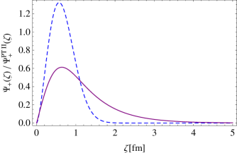
Figure 1: Comparison of the hyperbolic ground state wave function $\psi^{PTII}_{+}(\zeta)=\psi_{01\left(\frac{5}{2}\right)}(\zeta)$ in (56) (solid line) to the LFH wave function of equal quantum numbers, $\Psi_{+}^{01}(\zeta)$, in (60) (dashed line). We suppressed the upper indexes in the LFH wave function for the sake of keeping same notations as in GdTSBJ . The $\kappa$ and $\nu$ parameters have been taken same in both functions, and carry the values $\nu=1$, and $\kappa$= 2.14 fm^-1, respectively. The value of the radius of the hyperbolic function has to be consistent with the condition in (45), i.e. with $|s|>2n+|m|+1$, which determines the number of bound states within the potential under discussion. The radius is then deduced from our adopted $|s|=\frac{5}{2}$ value as $R=0.728$ fm. These are the parameters to be used in all subsequent calculations.

In the limit of small hyperbolic angles, which formally coincides with the limit of an increasing radius, $R\to\infty$, the equations (42)- (43) approach, modulo additive constants, the Light-Front Holographic equation (1). Indeed, it is not difficult to see that the $\textrm{ csch }^{2}\rho$ term approaches the inverse square distance potential, while the $\textrm{ sech }^{2}\rho$ potential goes to the harmonic oscillator according to,

$$\frac{1}{R^{2}}\frac{a(a-1)}{\sinh^{2}\rho} \longrightarrow a(a-1)\frac{1}{\zeta^{2}},\quad\rho=\frac{\stackrel{{\scriptstyle\frown}}{{z}}}{R},\quad\stackrel{{\scriptstyle\frown}}{{z}}\,\stackrel{{\scriptstyle R\to\infty}}{{\longrightarrow}}\,\zeta,$$ (48)

$$\kappa^{4}R^{2}{\tanh^{2}\rho} \longrightarrow \kappa^{4}R^{2}\frac{\stackrel{{\scriptstyle\frown}}{{z}}^{2}}{R^{2}}\longrightarrow\kappa^{4}\zeta^{2}.$$ (49)

Here, use has been made of the fact that the arc of the hyperbolic geodesic, $\stackrel{{\scriptstyle\frown}}{{z}}$, approaches the segment, $\zeta$, of a straight line. In effect, the form of the conformal interaction in (1), (2) is recovered as,

$$R\to\infty:\quad\frac{1}{R^{2}}\frac{a(a-1)}{\sinh^{2}\rho}-\frac{1}{R^{2}}\frac{\kappa^{4}R^{4}}{\cosh^{2}\rho}+\kappa^{4}R^{2}\longrightarrow\frac{a(a-1)}{\zeta^{2}}+\kappa^{4}\zeta^{2}.$$ (50)

This is in accord with (1), for $a$ becoming $\left(\nu+\frac{1}{2}\right)$. With that, the equivalence of the differential equations (42)–(44) and (1) (modulo the additive constants) has been demonstrated.

IV.2 Reproducing the LFH energies

Upon substituting again in (45)-(46) the $\lambda$ value from (44), the contraction limit of the energy is easily worked out as (see Alonso for a related consideration)

$$\lim_{R\to\infty}\left(\epsilon_{n}^{a\lambda}\right)^{Higgs}=\lim_{R\to\infty}\left[-\frac{1}{R^{2}}\left(\sqrt{\kappa^{4}R^{4}+\frac{1}{4}}-\left(\frac{1}{2}+a+2n\right)\right)^{2}+\kappa^{4}R^{2}+\frac{1}{R^{2}}\right]$$

$$\to\lim_{R\to\infty}\left[\kappa^{4}R^{2}-\frac{\left(2n+a+\frac{1}{2}\right)}{R^{2}}\left(\left(2n+a+\frac{1}{2}\right)-2\sqrt{{\kappa^{4}R^{4}}+\frac{1}{4}}+{\kappa^{4}R^{4}}+\frac{1}{4}\right)\right]$$

$$\longrightarrow 2\kappa^{2}\left(2n+a+\frac{1}{2}\right)=4\kappa^{2}\left(n+\frac{|m|+1}{2}\right),$$ (51)

with $a$ being substituted by $a=|m|+\frac{1}{2}$. We now recall that the energy in (51) has the dimensionality of fm^-2, i.e. $\left[\left({\epsilon}_{n}^{a\lambda}\right)^{Higgs}\right]={{\mathrm{f}}{\mathrm{m}}}^{-2}$, and coincides with the dimensionality of the quadratic energy in (26). Upon identifying $|m|$ with $\nu$, taking into account the rational units, $\hbar=1=2\mu$, and finally incorporating the additive constant $c_{+}^{\nu}=2\kappa^{2}(\nu+1)$ from (1) into (51), one finds that the contraction limit of the second Pöschl-Teller II potential on the hyperbola H${}_{+R}^{1}$ generates same spectrum as the Light-Front framework in (1), (2), namely,

$$\lim_{R\to\infty}\left(\epsilon_{n}^{a\lambda}\right)^{Higgs}+2\kappa^{2}(|m|+1) = 4\kappa^{2}\left(n+{|m|+1}\right)={E}^{2},\,|m|=\nu.$$ (52)

In conclusion, we demonstrated that the Light-Front holographic equation and its spectrum can, alternatively to AdS₂/CFT₁, be also traced back to the decreasing curvature (equivalently, small hyperbolic angle) limit of the Higgs oscillator on the hyperbolic plane H${}_{+R}^{2}$ , reduced to the one-dimensional Pöschl-Teller potential on the hyperbola ${\mathbf{H}}_{+R}^{1}$. In this fashion, the one dimensional Schrödinger equation of the holographic Light-Front QCD in the ${\mathcal{R}}^{1}$ space of the $\zeta$ variable has been recovered.

IV.3 Reproducing the LFH wave functions

In the following, the potential parameters $a$ and $\lambda$ in (44), which have been defined in (43) via their squares according to, $a(a-1)=|m|^{2}-\frac{1}{4}$, now with $a=\pm|m|+\frac{1}{2}$, and $\lambda(\lambda+1)=\kappa^{4}R^{4}$, with $\lambda=-\frac{1}{2}\pm\sqrt{\kappa^{4}R^{4}+\frac{1}{4}}$ will be chosen as,

$$a=-|m|+\frac{1}{2},\quad\lambda=-\frac{1}{2}-|s|,\quad|s|=\sqrt{{\kappa^{4}R^{4}}+\frac{1}{4}}.$$ (53)

This choice is compatible with the sign inversions of all the quantum numbers entering the definition of the energy, $\left(\epsilon_{n}^{a\lambda}\right)^{PTII}$, in (45). We now switch to more explicit (with respect to  (44)) labellings of the wave functions and energies as,

$$\psi_{n}^{a\lambda}(\rho)\longrightarrow\psi_{n|m||s|}(\rho),\quad\epsilon_{n}^{a\lambda}\longrightarrow\epsilon_{n|m||s|}.$$ (54)

In accord with (47) these wave functions now read,

$$\psi_{n|m||s|}(\rho)\sim\cosh^{\lambda+1}\rho\,\sinh^{|m|+\frac{1}{2}}_{2}F_{1}\left(-n,\left(-|s|-n+|m|+1\right),|m|+1,-\sinh^{2}\rho\right).$$ (55)

We first focus on the ground state wave function which is especially simple,

$$\psi^{PTII}_{+}\left({\zeta}\right):\Rightarrow\,\,\psi_{0|m||s|}(\rho)\sim\cosh^{-|s|+\frac{1}{2}}\rho\,\sinh^{|m|+\frac{1}{2}}\rho,\quad\rho=\frac{\zeta}{R}.$$ (56)

In making use of the approximation Alonso ,

$$\cosh\rho\approx\exp\left(\tanh^{2}\frac{\rho}{2}\right)\approx 1+\frac{1}{2}\rho^{2}\approx\exp\left(\frac{\rho^{2}}{2}\right),$$ (57)

the $R\to\infty$ limit of the $\cosh^{-\lambda+\frac{1}{2}}\rho$ factor easily calculates as,

$$\lim_{R\to\infty}\cosh^{-|s|}\rho \longrightarrow \exp\left(-|s|\tanh^{2}\frac{\rho}{2}\right)\longrightarrow\exp\left(-|s|\frac{\rho^{2}}{2}\right)$$ (58)

$$\longrightarrow \exp\left(-\kappa^{2}R^{2}\frac{\stackrel{{\scriptstyle\frown}}{{z}}\,^{2}}{2R^{2}}\right)\longrightarrow\exp\left(-\frac{\kappa^{2}\zeta^{2}}{2}\right),$$

where once again the arc of the geodesic, $\stackrel{{\scriptstyle\frown}}{{z}}$, approaches the segment, $\zeta$, of a straight line in the $R\to\infty$ limit. The $\left(\sinh^{2}\rho\right)^{\frac{m}{2}+\frac{1}{4}}$ factor behaves as,

$$\lim_{R\to\infty}\left(\sinh^{2}\rho\right)^{\frac{|m|}{2}+\frac{1}{4}}\sim\left(\zeta^{2}\right)^{\frac{|m|}{2}+\frac{1}{4}}.$$ (59)

Putting all together, the diminishing curvature limit of the ground state wave function $(|m|=1)$ of the second Pöschl-Teller potential is found as expected,

$$\Psi_{+}^{01}(\zeta):\Rightarrow\,\,\lim_{|s|\to\infty}\psi_{0|1||s|}(\rho)=Ne^{-\frac{\kappa^{2}\zeta^{2}}{2}}\left(\kappa^{2}\zeta^{2}\right)^{\frac{1}{2}+\frac{1}{4}},\quad|s|\approx\kappa^{2}R^{2},$$ (60)

where $N$ is a normalization constant. In this way, the $\Psi_{+}^{01}(\zeta)$ ground state in the Light-Front Holography following from (6) for $n=0$, and $\nu=1$ is recovered upon identifying as usual $|m|$ with $\nu$ (see Fig. 1). It is this wave function that is relevant for the description of the proton electric charge form factor below. Similarly, the remaining states can be analyzed. Indeed, in using the relationship between ${}_{2}F_{1}$ and ${}_{1}F_{1}$ hypergeometric functions, and the relationship of the Laguerre polynomials to ${}_{1}F_{1}$ Abramovic , jdcook , one finds the polynomial part of the wave function in (55) expressed in the following way in the $|s|\to\infty$ limit:

$${}_{2}F_{1}(-n,-|s|+n+1,|m|+1,-\sinh^{2}\rho)\stackrel{{\scriptstyle|s|\to\infty}}{{\longrightarrow}}\,_{1}F_{1}\left(-n,|m|+1,|s|\sinh^{2}\rho\right)$$

$$\stackrel{{\scriptstyle|s|\to\infty}}{{\longrightarrow}}\,_{1}F_{1}(-n,|m|+1,\kappa^{2}\zeta^{2})\sim L^{|m|}_{n}(\kappa^{2}\zeta^{2}).$$ (61)

Comparison to (6), and upon identifying once again $|m|$ with $\nu$, confirms that also the polynomial part for the “curved” wave functions in (55) approach the correct Laguerre polynomials defining the wave functions of the Light-Front Holographic equation, as it should be. In this fashion, the exact solutions to (1) from (6) are reproduced in the contraction limit of H${}_{+R}^{1}$ to a straight line on a cone (see also Alonso where the contraction limit of the Higgs oscillator on the hyperbola has been elaborated). As long as the inverse-square distance plus harmonic oscillator potential in one dimension represents a conformally invariant interaction, because the associated Hamiltonian is realized in terms of the $so(2,1)$ algebra elements in (27), a conformally symmetric interaction is found in the contraction limit.

IV.4 Reproducing the LFH proton electric charge form factor from the Fourier-Helgason hyperbolic wave transform

The proton electric charge form factor in the Conformal Light-Front Holographic QCD is well known and its calculation will not be reproduced here. Instead we explore utility of the hyperbolic wave function in (56) for the description of the same observable. The normalized ground state proton wave function reads,

$$\psi_{0|m||s|}(\rho)=\sqrt{\frac{2\Gamma(|s|)}{\Gamma(|m|+1)\Gamma(|s|-|m|-1)}}\cosh^{-|s|+\frac{1}{2}}\rho\sinh^{|m|}\rho,$$ (62)

Our calculation refers to a quark-diquark system of reduced mass $\mu$, as commented immediately after eq. (1) above. The adequate momentum space, dual to the curved position space on the hyperboloid, is obtained via the so called Fourier-Helgason integral transform IvaBogd based on the hyperbolic waves, also referred to in Alonso as Shapiro functions, $\Phi_{\mathbf{p}}^{(D)}({\mathbf{r}})$, with $D$ standing for the dimensionality of the surface. Specifically for the hyperboloid under investigation, $D=2$, they read,

$$\Phi_{\mathbf{p}}^{(2)}({\mathbf{r}}) = \left(\frac{x_{0}}{R}-\frac{\hat{\mathbf{p}}\cdot{\mathbf{r}}}{R}\right)^{-\frac{1}{2}-ipR},\quad{\mathbf{r}}=\left(\begin{array}[]{c}x_{1}\\ x_{2}\end{array}\right)=R{\hat{\mathbf{r}}}\sinh\rho.$$ (65)

Here, ${\hat{\mathbf{p}}}$ is the unit vector along the direction of the momentum ${\mathbf{p}}$ and tangent to the surface under consideration, $p$ is its magnitude, while ${\mathbf{r}}$ is the two-dimensional radius vector in the Euclidean $(x_{1},x_{2})\in{\mathcal{R}}^{2}$ plane. In making use of (33), the latter equation becomes,

$$\Phi_{\mathbf{p}}^{(2)}({\mathbf{r}}) = \left(\cosh\rho-\hat{\mathbf{p}}\cdot\hat{\mathbf{r}}\sinh\rho\right)^{-\frac{1}{2}-ipR},$$ (66)

$$= \left(e^{-\rho\hat{\mathbf{p}}\cdot\hat{\mathbf{r}}}\right)^{-\frac{1}{2}-ipR},\quad=e^{\frac{\rho}{2}\hat{\mathbf{p}}\cdot\hat{\mathbf{r}}}e^{i{\rho}{\mathbf{p}}\cdot R\hat{\mathbf{r}}}.$$

In recalling that the hyperbolic angle $\rho$ in (66) expresses in terms of the arc along a geodesic and the constant radius as, $\rho=\frac{\stackrel{{\scriptstyle\frown}}{{z}}}{R}$, amounts to the following equivalent expression for the Shapiro function (also see Ref. IvaBogd for more details),

$$\displaystyle{\Phi_{\mathbf{p}}^{(2)}({\mathbf{r}})=e^{\frac{\stackrel{{\scriptstyle\frown}}{{z}}}{2R}\hat{\mathbf{p}}\cdot\hat{\mathbf{r}}}e^{i\stackrel{{\scriptstyle\frown}}{{z}}{\mathbf{p}}\cdot\hat{\mathbf{r}}},\quad{\hat{\mathbf{p}}}\cdot\hat{{\mathbf{r}}}=\cos\varphi,}$$ (67)

where $\varphi$ is taken as the azimuthal angle in H${}_{+R}^{2}$ in (33). The latter expression shows that in the $R\to\infty$ limit, in which the hyperbolic geodesic stretches to a line of a direction given by ${\hat{\mathbf{r}}}$ in ${\mathcal{R}}^{2}$, the arc $\stackrel{{\scriptstyle\frown}}{{z}}$ approaches a corresponding line segment, $\zeta$. In this limit, the hyperbolic plane waves (the Shapiro functions) approach ordinary plane waves in a two-dimensional flat space and the integral transform correspondingly evolves to an ordinary two-dimensional Fourier transform,

$$\lim_{R\to\infty}\Phi_{\mathbf{p}}^{(2)}({\mathbf{r}})\longrightarrow e^{i{\mathbf{p}}\cdot{\mathbf{r}}}.$$ (68)

The Shapiro functions are normalized according to Alonso as,

$$\frac{R}{2\pi}\int_{{\mathbf{r}}\in{\mathcal{R}}^{2}}\frac{{\mathrm{d}}^{2}{\mathbf{r}}}{x_{0}}\Phi^{(2)}_{{\mathbf{p}}}\,{}^{\ast}({\mathbf{r}})\Phi_{{\mathbf{p}}^{\prime}}^{(2)}(\mathbf{r}) = N^{(2)}(p)\delta^{(2)}({\mathbf{p}}-{\mathbf{p}}^{\prime}),$$

$$\frac{R}{2\pi}\int_{{\mathbf{p}}\in{\mathcal{R}}^{2}}\frac{{\mathrm{d}}^{2}{\mathbf{p}}}{N^{(2)}(p)}\Phi^{(2)}_{{\mathbf{p}}}\,{}^{\ast}({\mathbf{r}})\Phi_{{\mathbf{p}}}^{(2)}({\mathbf{r}}^{\prime}) = \delta^{(2)}({\mathbf{r}}-{\mathbf{r}}^{\prime}),$$

In terms of the Shapiro functions, the momentum space for the hyperboloid is defined according to Alonso , IvaBogd ,

$$F({\mathbf{p}}) = \frac{R}{2\pi}\int_{{\mathbf{r}}\in{\mathcal{R}}^{2}}\frac{{\mathrm{d}}^{2}{\mathbf{r}}}{x_{0}}\Phi^{(2)}_{{\mathbf{p}}}\,{}^{\ast}({\mathbf{r}})f(\mathbf{r}),$$

$$f({\mathbf{r}}) = \frac{R}{2\pi}\int_{{\mathbf{p}}\in{\mathcal{R}}^{2}}\frac{{\mathrm{d}}^{2}{\mathbf{p}}}{N^{(2)}(p)}\Phi_{{\mathbf{p}}}^{(2)}({\mathbf{p}})F({\mathbf{p}}).$$ (70)

Within this framework, the proton electric form factor on the hyperbolic space is obtained as a Fourier-Helgason transform of the squared ground state wave function in (62) (with the “curved” wave function containing a $\sqrt{\sinh\rho}$ less than the Schrödinger one according to (33), as

$$G_{E}^{p}({Q^{2}})=R^{2}\int_{0}^{\infty}{\mathrm{d}}\rho\,\frac{\sinh\rho}{\cosh\rho}\frac{|\psi_{01|s|}(\rho)|^{2}}{\sinh\rho}\int_{-\pi}^{+\pi}{\mathrm{d}}\varphi e^{\frac{\rho\cos\varphi}{2}}e^{iQR\rho\cos\varphi}$$ (71)

$$\approx\int_{0}^{\infty}{\mathrm{d}}\,\rho\cosh^{-2|s|+1}\rho\,\sinh^{2}\rho\,e^{\frac{\rho}{2}}\int_{-\pi}^{+\pi}{\mathrm{d}}\varphi e^{iQR\rho\cos\varphi},\,\,\cos\varphi={\hat{\mathbf{q}}}\cdot{\hat{\mathbf{r}}},$$ (72)

where ${\hat{\mathbf{q}}}$ is the unit vector along the transferred momentum, and $Q^{2}=-{\mathbf{q}}^{2}$. In order to obtain a closed value for $G_{E}^{p}({Q^{2}})$, we ignored presence of $|\cos\varphi|\leq 1$ in the real exponential factor, i.e, we replaced $e^{\frac{\rho}{2}\cos\varphi}$ by $e^{\frac{\rho}{2}}$. This allows us to carry out the integration over the azimuthal angle as AW

$$\frac{1}{2\pi}\int_{0}^{2\pi}e^{i\rho QR\cos\varphi}{\mathrm{d}}\varphi=J_{0}(QR\rho),\quad Q=|{\mathbf{q}}|.$$ (73)

Next we are interested in relatively small angles in view of the rapid decrease of the ground sate wave function with $\rho$ as illustrated by Fig. 1. With that in mind, we keep only the lowest terms in the $\exp(\rho/2)$ expansion, and approximate the $\sinh\rho$ from the integration volume by $\rho$, which allows us to convert the Fourier-Helgason transform to a Hankel transform. Finally, in systematically making use of eq. (57) to replace everywhere $\cosh\rho$ by $\exp(\rho^{2}/2)$, and make use of $\tanh\rho\stackrel{{\scriptstyle R\to\infty}}{{\longrightarrow}}1$ allows to simplify the equation (72) as,

$$G_{E}^{p}({Q^{2}}) = R^{2}\int_{0}^{\infty}{\mathrm{d}}\rho\,e^{-\frac{3}{2}\rho^{2}}\left(1+\frac{\rho}{2}\right)\rho\,J_{0}(QR\rho).$$ (74)

The latter integral takes in closed form by means of the symbolic software Mathematica and reads,

$$G_{E}^{p}({Q^{2}})=\frac{R^{2}}{2}\,e^{-\frac{Q^{2}R^{2}}{6}}\left(1-\frac{1}{12}\sqrt{\frac{\pi}{6}}\left[(Q^{2}R^{2}-6)I_{0}\left(\frac{Q^{2}R^{2}}{12}\right)-Q^{2}R^{2}I_{1}\left(\frac{Q^{2}R^{2}}{12}\right)\right]\right),$$ (75)

where $I_{0}$ and $I_{1}$ denote the modified Bessel functions of zeroth and first degree, correspondingly.

• In this fashion, the proton electric charge form-factor has been calculated within a hyperbolic quark-diquark model suited for dynamics in the ultraviolet and respecting in the flat-space limit the conformal symmetry.

The observable obtained is displayed in Fig. 2, where it has been compared to same physical entity, earlier calculated in the infrared in TQC once again employing a conformal quark-diquark model, namely the one based on the trigonometric Rosen-Morse potential. The Figure  3 shows the behavior of both form factors under discussion with the increase of the momentum transferred. Finally, in Fig. 4 we display the approximate and exact hyperbolic integrands corresponding to (72). The model employed in the ultraviolet and elaborated here is placed on a non-compact (1+2) Minkowski space, ${\mathbf{H}}_{+R}^{2}$ and in accord with the relativistic nature of the ultraviolet (ultra-relativistic) regime of QCD. The small hyperbolic approximation used guarantees conformal symmetry in accord with LFH. Instead, the previously developed model in the infrared, that has been used as a comparison, is placed on the compact version of ${\mathbf{H}}_{+R}^{3}$ which is the hyperspherical space, $S^{3}_{R}$, as more appropriate in the near rest-frame regime. The conformal symmetry of the $\csc^{2}$ piece is obvious from the fact that it appears as a part of the Laplace-Beltrami operator on $S^{3}_{R}$ and defines the free motion there. The perturbation by the cotangent term, a harmonic function on the surface under consideration, also known as “curved” Coulomb perturbance, conserves the conformal algebra. The reason is that the Hamiltonian describing such a motion can be cast in the form of a Casimir invariant of a non-trivial representation of the $so(4)$ sub-algebra of the conformal algebra $so(2,4)$, a result due to PalKi . Both form-factors obviously compare in quality and go practically through the data, not shown here (see Data_FF ,TQC and references therein). The coincidence of the two form-factors strongly points on conformal symmetry as the chief designer of quark dynamics in the two extreme QCD regimes.

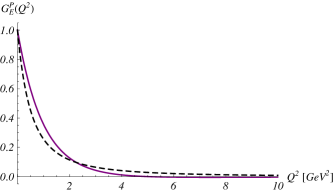
Figure 2: Side by side comparison of the proton electric charge form factor, $G^{p}_{E}(Q^{2})$, predicted by two distinct conformal quark-diquark models, the one elaborated here and suited for the ultraviolet regime of QCD (solid line), and another one, earlier presented in TQC and relevant in the infrared regime (dashed line). The calculation in the ultraviolet has been performed in (75) in terms of the small angle approximation to the ground state wave function of the Pöschl-Teller II potential and using a Fourier-Helgason transform of the charge-density, while the one in the infrared is based on the wave function of the trigonometric Rosen-Morse potential, a $\csc^{2}+\cot$ interaction and the equation (81) given in the Appendix.

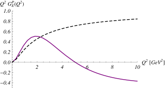
Figure 3: Comparison of the behaviors of $Q^{4}G^{p}_{E}(Q^{2})$, calculated in the ultraviolet with the small angle approximation to ground state wave function of the second hyperbolic Pöschl-Teller potential in (56) (solid line), and in the infrared with the one corresponding to the conformal trigonometric Rosen-Morse potential in TQC (dashed line). Notice the correct increase near origin, shared by both form factors.

Finally, the behavior of $Q^{4}G^{p}_{E}(Q^{2})$ near origin displayed in Fig. 3 is once again illustrative of the proximity of the small hyperbolic angle approximation to the Pöschl-Teller II wave functions to the conformally invariant Light-Front Holographic ones. At high momentum transfers, however, only the form factor corresponding to the infrared shows the desired scaling property. The divergence of the form-factor in our hyperbolic model is understandable in view of the circumstance that its conformal symmetry is limited to small angles.

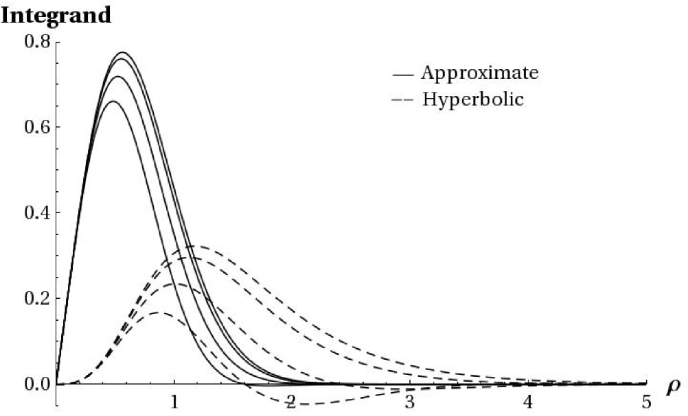
Figure 4: Approximate (74) (solid line) and exact (71)-(72) (dashed line) integrands. The various integrands correspond from bottom to top to decreasing $Q=3,2,1,0$ values (in GeV). The small differences between the areas under the solid–, and dashed line curves of same $Q$’s are illustrative of the reasonable accuracy of the small angle approximation in the evaluation of the Fourier-Helgason integral transform.

V Conclusions

In this work we studied the Higgs oscillator on the hyperbolic plane, reduced to the 1D Schrödinger equation describing motion on a hyperbola perturbed by the second hyperbolic Pöschl-Teller potential. In considering the decreasing curvature limit, equivalent to small hyperbolic angles, we found in eqs. (48)–(49) that this potential amounted to the one dimensional conformally symmetric interaction consisting of an inverse square distance plus a square distance potentials. In this fashion, the Lorentz symmetry of the initial hyperbolic interaction (i.e. $\ell(\ell+1)/\sinh^{2}\rho$ in (32)), that has been broken by the perturbation due to the Higgs oscillator in (42)-(44), to the end has been converted to conformal interaction in the flat space limit. Comparison of the Light Front Holographic ground state wave function in (60) to the hyperbolic one in (62) was presented in Fig. 1. We observed that for a relatively short radius, of the order of $1$ fm, the wave functions coincided quite reasonably. Such is due to the fact that the most essential part of the LFH wave function is located in the small distance region, comparable to small angles on the curved surface. Within same scheme, we also studied the proton electric charge form factor, shown in Figs. 2 and  3, and found again a pretty realistic data description in terms of a Fourier-Helgason transform of the charge density. In result, we found that essential outcomes of the Light-Front Holographic QCD in the ultraviolet can independently be backed up by a hyperbolic relativistic quark-diquark ($q-(qq$)) model, consistent with conformal symmetry. The model parallels in the ultraviolet another one, earlier developed in the infrared, and in which the $q-(qq)$ system, placed on the compact space of the hypersphere $S^{3}_{R}$, interacts via the “curved” Coulomb potential, a cotangent function of the second polar angle. This function is part of the standard trigonometric Rosen-Morse potential Manning_Rosen (see the Appendix for details). The cotangent potential has been shown in PalKi to be generated by the Casimir invariant of the $so(4)$ algebra in a representation nonequivalent to the canonical, a reason for which it represents a conformal interaction. In this fashion, we showed that the conformal symmetry, the decisive mechanism in shaping the light flavor hadron spectra and the electric charge form factor, can be treated on similar terms in the two extreme regimes of QCD. Spaces of constant curvatures, are known to efficiently absorb part of the interactions into the free motion, and frequently happen to provide convenient scenarios for the description of complex dynamical systems IvaBogd . Such models can further be upgraded by perturbations of the free motions and in this fashion the level of phenomenological description of coupled systems can be improved. The inverse radius of the H${}^{2}_{+R}$ space of constant curvature considered here provides a second scale in addition to the strength of the perturbing potential and can be employed in the definition of chemical potential along the lines of Refs. Ebert ,Anim .

• In summary, in the ultraviolet, as well as in the infrared, the conformal symmetry of the Schrödinger equations has been realized in the presence of two external length scales, brought about by the respective potential strengths, on the one side, and by the curvatures of of the respective relevant hosting curved mannifolds, on the other side.

The findings reveal the possibility that a new generation of quark models based on trigonometric or hyperbolic SUSY-QM potentials is capable of capturing notably more of the essential field-theoretical–, and first-principle AdS/CFT aspects of QCD in the infrared and the ultraviolet than models based on the traditional power potentials.

VI Appendix: The trigonometric Rosen-Morse potential

In this Appendix we summarize for the sake of completeness of the presentation the basics of the quark-diquark model with the trigonometric Rosen-Morse potential, closely following Refs. TQC , PRD10 . The model can be formulated both in three dimensional flat space, and on the three dimensional hypersphere, $S^{3}$. The flat-space interaction under consideration is given as,

$${\mathcal{V}}_{RMt}\left(\frac{r}{d}\right)=\frac{1}{d^{2}}\ell(\ell+1)\csc^{2}\left(\frac{r}{d}\right)-2\frac{b}{d^{2}}\cot\left(\frac{r}{d}\right),\quad b=\frac{2\mu dG}{\hbar^{2}}.$$ (76)

In flat space, $d$ is only a matching length parameter, while for a ${\mathcal{V}}_{RMt}$ placed on a compact hyperspherical surface, $S^{3}_{R}$, it acquires meaning of the constant hyper-radius $R=d$. On $S^{3}_{R}$, the $\csc^{2}$ term is absorbed into the Laplace-Beltrami operator and thereby into the free motion. The remaining cotangent term, is a harmonic function on $S^{3}_{R}$, a reason for which it is frequently referred to as “curved” Coulomb. The Hamiltonian, ${\mathcal{H}}_{RMt}$, describing in the equivalent one dimensional Schrödinger equation such a motion, can be shaped as a Casimir invariant, ${\widetilde{\mathcal{K}}}$, of a non-trivial representation of the $so(4)$ sub-algebra of the conformal $so(2,4)$, a result reported in PalKi . For the ground state, this representation is specifically simple and is given by,

$${\mathcal{H}}_{RMt}={\widetilde{\mathcal{K}}}-b^{2}, {\widetilde{\mathcal{K}}}=\sin^{-1}\chi e^{-b\chi}\,{\mathcal{K}}e^{b\chi}\,\sin\chi,$$ (77)

where ${\mathcal{K}}$ is the regular geometric $so(4)$ Casimir operator on $S^{3}_{R}$, $\chi$ is the second polar angle in the parametrization of the hypersphere. Important, the first terms in the Taylor series expansion of ${\mathcal{V}}_{RMt}$, coincide with the Cornell potential, predicted by Lattice QCD, in the presence of a centrifugal barrier, i.e. with

$${\mathcal{V}}_{RMt}\left(\frac{r}{d}\right) \approx \frac{\ell(\ell+1)}{r^{2}}-\frac{4\mu G}{\hbar^{2}r}+\frac{4\mu G}{3\hbar^{2}d^{3}}r,$$ (78)

$$\lim_{d\to\infty}{\mathcal{V}}_{RMt}\left(\frac{{r}}{d}\right) \longrightarrow \frac{\ell(\ell+1)}{r^{2}}-\frac{4\mu G}{\hbar^{2}r}.$$ (79)

In case ${\mathcal{V}}_{RMt}$ where to be considered on the hypersphere, the radial distance, $r$, would become $\stackrel{{\scriptstyle\frown}}{{r}}$, the arc of an $S^{3}_{R}$ geodesic and $d$ would take the place of the hyper-radius, $R$. As visible from eq. (79), in the flat space limit, ${\mathcal{V}}_{RMt}$ approaches the inverse distance potential, i.e. again a conformal interaction. In this manner, the trigonometric Rosen-Morse potential is conformally invariant in both curved- and flat spaces. This is different from the case of the Higgs oscillator potential problem on the hyperbolic plane, which acquires conformal symmetry exclusively in the flat space limit.

• In effect, the trigonometric Rosen-Morse potential provides a through and through conformal interaction in the infrared and is a manifest example for the possibility of realizing conformal symmetry in the presence of two scales– the strength of the cotangent term, $G$, and the length parameter $d$, equivalent to the hyperspherical radius $R$. The last scale allows for the introduction of temperature as the inverse hyper-radius, $T=1/R$ Tim .

Though the potential under discussion captures essential relativistic features brought about by the local isomorphism between $so(4)$ and the Lorentz algebra $so(1,3)$, such as the dimensionality of the irreducible representation functions, in operating on a compact manifold, and in having infinitely many bound states, it is at the same time closely tied to near rest-frame physics. In effect, this potential gives rise to a conformal spectrum of hydrogen-like degeneracy patterns, according to

$$\frac{2\mu E^{RMt}_{n\ell}}{\hbar^{2}}=-\frac{4\mu^{2}G^{2}}{\hbar^{4}\left(n+\ell+1\right)^{2}}+\frac{1}{d^{2}}(n+\ell+1)^{2}\stackrel{{\scriptstyle d\to\infty}}{{\longrightarrow}}-\frac{4\mu^{2}G^{2}}{\hbar^{4}\left(n+\ell+1\right)^{2}},$$ (80)

again in the units of fm^-2 used through the paper. The latter equation makes manifest one more difference between the trigonometric quark model in the infrared and the hyperbolic one in the ultraviolet. The issue is that while in the ultraviolet setup the physical spectrum is explained by the small hyperbolic angle limit to Pöschl-Teller II in (51), in the infrared it requires the full angular range of the trigonometric Rosen-Morse potential. The latter spectrum matches well the observed degeneracies in both the non-strange baryon- and meson excitations in the 1500 MeV to 2500 MeV range, a phenomenon whose appearance is justified by the opening of the conformal window Andre in the infrared. Moreover, upon being employed as a gauge potential in the Klein-Gordon scale equation on the three dimensions hypersphere, $S^{3}$, it furthermore provided a realistic description of the $P_{2I,1}$–$S_{2I,1}$ orderings through the entire known $N$ and $\Delta$ spectra as a kinematic splitting effect PRD10 . Within this framework, the respective protob charge-electric form factor, $G_{E}^{p}(Q^{2})$, has been predicted as,

$$G_{E}^{p}(Q^{2}) = \frac{b(b^{2}+1)}{Qd}\tan^{-1}\frac{16bdQ}{(Qd)^{4}+4(2b^{2}-1)(Qd)^{2}+16b^{2}(b^{2}+1)},$$ (81)

with $b$ from (76). The $b$ and $d$ values are those given in TQC .

Acknowledgment: We thank Cliffor Compean for the critical reading of the manuscript and valuable comments.

References

- (1) F. Cooper, A. Khare, and U. Sukhatme, Supersymmetry and quantum mechanics, Phys. Rept. 251 (1995) 267-385.
- (2) S. J. Brodsky, G. de Téramond, and M. Karliner, Puzzles in hadron physics and novel Quantum Chromodynamics phenomenology, Ann. Rev. Nucl. Part. Sci. 62 (2012) 1-35.
- (3) Guy F. de Téramond and S. J. Brodsky, The hadronic spectrum of a holographic dual QCD, Phys. Rev. Lett. 94 (2005) 201601.
- (4) A. Karch, E. Katz, D. T. Son, and M. A. Stephanov, Linear Confinement and AdS/QCD, Phys. Rev. D 74 (2006) 015005.
- (5) S. J. Brodsky, Guy F. de Téramond, and H.-G. Dosch, Threefold complementary approach to holographic QCD, Phys. Lett. B 729 (2014) 3-8.
- (6) J. L. F. Barbón and C. A. Fuertes, On the spectrum of non-relativistic AdS/CFT, JHEP 0809:030 (2008).
- (7) C. Leiva and M. S. Plyushchay, Conformal symmetry of relativistic and non-relativistic systems and AdS/CFT correspondence, JHEP 0310 (2003) 69.
- (8) G. B. Arfken and H.-J. Weber, Mathematical Methods for Physicists (Academic Press, N.Y. 2001).
- (9) M. Kirchbach, Conformal symmetry algebra of the quark potential and degeneracy in hadron spectra, AIP Conf. Proc. 1488 (2012) 236-247.
- (10) M. F. Manning and N. Rosen, Potential functions for vibrations of diatomic molecules, Phys. Rev. 44 (1933) 951-954.
- (11) P. W. Higgs, Dynamical symmetries in a spherical geometry, J. Phys A:Math.Gen. 12 (1979) 309-323.
- (12) F. Cooper, J. N. Ginochio, and A. Wipf, Supersymmetry, operator transformations and exactly solvable potentials, J. Phys. A:Math.Gen. 22 (1989) 3707-3716.
-
(13)
A. O. Barut, A. Inomata, and R. Wilson,
Algebraic treatment of the second Pöschl-Teller Morse-Rosen and Eckart equations,
J. Phys. A:Math.Gen. 20 (1987) 4083-4096;
F. M. Solikhah, Suprami, and V. I. Variani, Analysis of energy spectrum and wave functions of modified Pöschl- Teller potential using hypergeometry and supersymmetric method, IPTEK, The Journal for Technology and Science, 23 (2012) 15-20. - (14) S. D. Avramis, K. Sfetsos, and K. Siompos, Stability of string configurations dual to quarkonium states in AdS/CFT, Nucl. Phys. B 793 (2008) 1-33.
- (15) M. A. Alonso, G. S. Pogosyan, and K. B. Wolf, Wigner functions for curved spaces.I.On hyperboloids, J. Math. Phys. 43(12) (2002) 5857-5871.
- (16) M. Abramovicz and I. A. Stegun, Handbook of Mathematical Functions, with Formulas, Graphs and Mathematical Tables,, Dover Publications, Inc. N.Y. 1972 .
-
(17)
John D. Cook, Relations between special functions,
http://www.johndcook.com/special-function-diagram.html - (18) Iva Bogdanova, Pierre Vandergheynst, and Jean-Pierre Gazeau, Continuous wavelet transform on the hyperboloid, Applied and Computational Harmonic Analysis, 23 (3) (2007) 285-306.
- (19) C. Compean and M. Kirchbach, Trigonometric quark confinement potential of QCD traits, Eur. Phys. J. A 33 (2007) 1-4.
- (20) A. Pallares-Rivera and M. Kirchbach, Symmetry and degeneracy of the curved Coulomb potential on the ball, J. Phys. A:Math.Theor. 44 (2011) 44530.
- (21) J. Friedrich and Th. Walcher, A coherent interpretation of the form factors of the nucleon in terms of a pion cloud and constituent quarks, Eur. Phys. J. A 17 (2003) 607-623.
- (22) S. Hands, T. J. Hollowood, and J. C. Myers, QCD with Chemical Potential in a small hyperspherical box, JHEP 1007 (2010) 086.
- (23) A. Deur, V. Burkert, J. P. Chen, and W. Korsch, Determination of the effective strong coupling constant from CLAS spin structure function data, Phys. Lett. 665 (2008) 349-351.
- (24) M. Kirchbach and C. B. Compean, Conformal symmetry and light flavor baryon spectra, Phys. Rev. D 82 , 034008(2010).
- (25) D. Ebert, A. V. Tykov, and V. Ch. Zhukovsky, Gravitational catalysis of chiral and color symmetry breaking of quark matter in hyperbolic space, JHEP 0902 (2009) 028.
- (26) D. Krioukov, F. Papadopoulos, A. Vahdat, and M. Boguna, Curvature and temperature of complex networks, Phys. Rev. E 80 (2009) 035101.