Thermoelectric effect enhanced by the resonant states in graphene

Abstract

Thermoelectric effects in graphene are considered theoretically with particular attention paid to the role of impurities. Using the $T$-matrix method we calculate the impurity resonant states and the momentum relaxation time due to scattering on impurities. The Boltzmann kinetic equation is used to determine the thermoelectric coefficients. It is shown that the resonant impurity states near the Fermi level give rise to a resonant enhancement of the Seebeck coefficient and of the figure of merit $ZT$. The Wiedemann-Franz ratio deviates from that known for ordinary metals, where this ratio is constant and equal to the Lorentz number. This deviation appears for small chemical potentials and in the vicinity of the resonant states. In the limit of a constant relaxation time, this ratio has been calculated analytically for $\mu=0$.

I Introduction

Graphene, the first strictly two-dimensional crystal, has been extensively studied, both experimentally and theoretically. This enormous interest in graphene results mainly from peculiar transport properties, which follow from its very specific electronic structure. Thermal and thermoelectric properties of graphene have become a topical issue since the first measurement of thermal conductivity in graphene by Balandin et al. balandin2008 It is known that graphene is one of the best heat conductors, with a very high thermal conductivity that is a consequence of the strong $sp^{2}$ bonding, light atomic mass, and low dimensionality. Xu2014 A giant thermoelectric effect in graphene was also predicted theoretically, Dragoman with the Seebeck coefficient equal to 30 mV/K.

Impurities can substantially influence graphene’s energy spectrum, so the thermoelectric transport strongly depends not only on the thermal activation but also on the impurity scattering. The influence of impurity scattering on the thermoelectric properties of graphene was considered theoretically using a self-consistent t-matrix approach by Lofwander et al.Lofwander From these considerations follows that the measured thermopower can be used to get some information on the role of impurity scattering in graphene. The thermopower near the Dirac point was considered by Wang et al,Wang who obtained a relatively good agreement between experimental data and theoretical results based on the Boltzmann transport theory. These authors also showed that the Mott’s relation fails in the vicinity of the Dirac points in the case of high-mobility graphene, being however satisfied for a wide range of gate voltages in the regime of low carrier mobility. The thermoelectric transport in graphene was also considered for Dirac fermions in the presence of magnetic field and disorder  Zuev ; Zhu ; Yan .

Sharapov et al Sharapov have found that the thermopower can be remarkably enhanced by opening an energy gap in the quasiparticle spectrum of graphene. The presence of energy gap is accompanied by the emergence of quasiparticle scattering channel, with the relaxation time strongly dependent on energy. The thermoelectric effects ware also investigated in multilayer graphene systems. The thermopower of biased and unbiased multilayer graphene was studied in the Slonczewski-Weis-McClure model, where the effect of impurity scattering was treated in the self-consistent Born approximationhao . The classic and spin Seebeck effects in single as well as in multilayer graphene on the SiC substrate were also investigated within ab-initio methods, Wierzbowska1 ; Wierzbowska2 and by nonequilibrium molecular-dynamics simulations. fthenakis

Transport properties of graphene nanoribbons (GNRs) can differ from the corresponding ones of a two-dimensional graphene plane, mainly due to edge sates and energy gaps which develop in the electronic spectrum. These transport properties also depend on the edge shape. Thermoelectric properties of GNRs have also been investigated and it has been shown that thermopower in GNRs can be remarkably larger than that in the planar graphene.wei Moreover, the corresponding figure of merit, $ZT$, can be enhanced by introducing randomly distributed hydrogen vacancies into completely hydrogenated GNRs.liang Structural defects, especially in the form of antidots, were also shown to be a promising way of enhancing thermoelectric efficiency in GNRs.gunst ; karamitaheri ; yan ; chang ; wierzbicki

In this paper we consider thermoelectric properties of a two-dimensional graphene with impurities which lead to resonant states near the Fermi level. We show that the resonant states result in resonant enhancement of the Seebeck coefficient. This enhancement can be observed when the Fermi level is tuned by an external gate voltage. In section 2 we describe the model and theoretical method used to calculate the Seebeck coefficient. The relaxation time is calculated in section 3. Numerical results on the thermoelectric transport properties are presented and discussed in section 4. Wiedemann-Franz law is briefly discussed in section 5, wile final conclusions are in section 6.

II Model

In a clean (defect-free) graphene, the electronic states in the vicinity of the Dirac points can be described by the following low-energy Hamiltonian kane

$$\hat{H}_{0}=-i\hbar v\,(\sigma_{x}\nabla_{x}+\sigma_{y}\nabla_{y})\,,$$ (1)

where $v$ is the electron velocity in graphene, and $\sigma_{x}$, $\sigma_{y}$ are the Pauli matrices defined in the two-sublattice space of graphene. This Hamiltonian describes two electron energy bands with linear dispersion, $\varepsilon^{(1,2)}({\bf k})=\pm\hbar vk$. The electron velocity in each of the bands is $\mathcal{\bf v}^{(1,2)}({\bf k})=\pm v{\bf k}/\ k$.

Assume that a temperature gradient $\nabla T$ and external electric field $E$ are oriented along the axis $x$. Both, $\nabla T$ and $E$ drive the system out of equilibrium. To calculate the distribution function $f^{(n)}({\bf r,k})$ of electrons in the $n$-th energy band in the nonequilibrium situation, we apply the Boltzmann kinetic equation. For a weak deviation $\delta f^{(n)}$ of the distribution function from the equilibrium distribution $f_{0}$, the Boltzmann equation for $\delta f^{(n)}$ can be written in the relaxation time approximation as

$$v^{(n)}_{x}\,\left(-\frac{\partial f_{0}}{\partial\varepsilon}\right)\,\left(\nabla\mu+\frac{\varepsilon-\mu}{T}\;\nabla T-eE\right)=-\frac{\delta f^{(n)}}{\tau^{(n)}}\,,$$ (2)

where $f^{(n)}({\bf r,k})=f_{0}+\delta f^{(n)}$, $\tau^{(n)}$ is the relaxation time in the $n$-th band, while $\mu$ is the chemical potential, which may be spatially inhomogeneous along the axis $x$ and thus $\nabla\mu=\partial\mu/\partial x$ is a driving force as well.

Using the solution of Eq. (2), one can find the electric current density $j$ and the energy flux density $J_{E}$ along the axis $x$, induced by the driving forces $E$, $\nabla T$, and $\nabla\mu$,kireev

$$j=e\sum_{n{\bf k}}v^{(n)}_{x}\delta f^{(n)}=e^{2}K_{11}E\hskip 28.45274pt$$

$$-eK_{11}T\,\nabla\frac{\mu}{T}-eK_{21}\frac{\nabla T}{T}\,,$$ (3)

$$J_{E}=\sum_{n{\bf k}}v^{(n)}_{x}\varepsilon^{(n)}\,\delta f^{(n)}=eK_{21}-K_{21}T\,\nabla\frac{\mu}{T}-K_{31}\frac{\nabla T}{T}\,,$$ (4)

where $K_{rs}$ are the kinetic coefficients for graphene

$$K_{rs}=-\frac{1}{4\pi\hbar^{2}}\int_{-\infty}^{\infty}|\varepsilon|\,\varepsilon^{r-1}\tau^{s}(\varepsilon)\,\frac{\partial f_{0}}{\partial\varepsilon}\,d\varepsilon.$$ (5)

The integral in Eq.(5) runs over both energy bands, so $\tau(\varepsilon)$ is equal to $\tau^{(1)}(\varepsilon)$ for $\varepsilon>0$, and $\tau^{(2)}(\varepsilon)$ for $\varepsilon<0$, respectively. Note, that the heat current density $J_{Q}$ is defined as $J_{Q}=J_{E}-\mu j$, so that $J_{Q}=J_{E}$ when $j=0$.

The thermoelectric Seebeck coefficient $\alpha$ and the heat conductivity $\kappa$ are defined from the relations $E^{\alpha}=\alpha\nabla T$ and $J_{Q}=-\kappa\nabla T$ when $j=0$, where $E^{\alpha}$ is the electric field due to the temperature gradient. In general, there is also a field related to the chemical potential inhomogeneity, $E^{\mu}=\nabla\mu/e$, so that the total internal electric field for $j=0$ is $E=E^{\mu}+E^{\alpha}$. This leads to the standard expressions for the electrical conductivity $\sigma$, thermoelectric Seebeck coefficient $\alpha$, and heat conductance $\kappa$ kireev

$$\sigma=e^{2}K_{11},$$ (6)

$$\alpha=\frac{K_{21}-\mu K_{11}}{e\,TK_{11}}$$ (7)

$$\kappa=\frac{K_{31}K_{11}-K_{21}^{2}}{TK_{11}},$$ (8)

which are valid for graphene when the kinetic coefficients $K_{rs}$ are calculated from Eq. (5).

To calculate the thermoelectric parameters, Eqs(6-8), it is necessary to know the energy dependence of the relaxation time due to electron scattering from impurities and defects. This problem is considered in the section below.

III Momentum relaxation time

The total Hamiltonian of graphene with impurities is $\hat{H}=\hat{H}_{0}+\sum_{i}\hat{V}({\bf r-R}_{i})$, where $\hat{V}({\bf r-R_{i}})$ is a scattering potential of a single impurity located at ${\bf R}_{i}$, and the sum goes over all randomly distributed impurities. We consider the situation, when the short-range-potential impurities are distributed randomly with equal probabilities in the sublattices A and B of the graphene. Correspondingly, the single-impurity perturbation is either $\hat{V}^{A}({\bf r})$ or $\hat{V}^{B}({\bf r})$, where

$$\hat{V}^{A,B}({\bf r})=\hat{V}_{0}^{A,B}\,\delta({\bf r}-{\bf R}_{A,B}),$$ (9)

where $\hat{V}_{0}^{A,B}=V_{0}(\sigma_{0}\pm\sigma_{z})/2$, $V_{0}$ is the impurity potential strength, $\sigma_{0}$ is the unit matrix in the sublattice space and ${\bf{R}}_{A}$ (${\bf{R}}_{B}$) is a position vector of the impurity if it is in the sublattice A (B).

The influence of a single impurity on the energy spectrum and on the momentum relaxation time can be described in terms of the T-matrix method mahan . The T-matrix equation in the general case takes the form

$$\hat{T}_{\bf kk^{\prime}}(\varepsilon)=\hat{V}_{\bf kk^{\prime}}+\sum_{\bf k^{\prime\prime}}\hat{V}_{\bf kk^{\prime\prime}}\hat{G}_{\bf k^{\prime\prime}}(\varepsilon)\,\hat{T}_{\bf k^{\prime\prime}k^{\prime}}.$$ (10)

where

$$\hat{G}_{\bf k}(\varepsilon)=\frac{\varepsilon+\mbox{\boldmath$\sigma$}\cdot{\bf k}}{(\varepsilon+i\delta)^{2}-(\hbar vk)^{2}}$$ (11)

is the retarded Green’s function of electrons in graphene described by the Hamiltonian $\hat{H}_{0}$.

In the case of short-range impurities, we can find from Eq. (10) the T-matrix in the following form

$$\hat{T}^{A,B}(\varepsilon)=\frac{\hat{V}^{A,B}_{0}}{1-V_{0}F(\varepsilon)}\,,$$ (12)

where $F(\varepsilon)$ is defined as

$$F(\varepsilon)=\sum_{\bf k}\frac{\varepsilon}{(\varepsilon+i\delta)^{2}-(\hbar vk)^{2}}\,.$$ (13)

Using Eq. (12), and averaging over the impurity positions (assuming the same probability to find impurity in the sublattice A or B), we can find the self-energy of electrons due to the scattering from impurities

$$\hat{\Sigma}(\varepsilon)=\frac{N_{i}V_{0}\,\sigma_{0}}{2\,[1-V_{0}F(\varepsilon)]}\,,$$ (14)

where $N_{i}$ is the impurity concentration.

To find the relaxation time of electrons in the energy bands 1 and 2, we have to diagonalize the operator $\hat{H}_{eff}\equiv\hat{H}_{0}+\hat{\Sigma}(\varepsilon)$. Since the self energy (14) is proportional to the unit matrix $\sigma_{0}$, the operator $\hat{H}_{eff}$ is diagonalized by the same transformation as $\hat{H}_{0}$. In other words, the relaxation time of electrons in graphene can be found directly from Eq. (14) by using relation

$$\frac{\hbar}{\tau(\varepsilon)}={\rm Im}\;\frac{N_{i}V_{0}}{1-V_{0}F(\varepsilon)}\,.$$ (15)

It can be also presented as

$$\frac{\hbar}{\tau(\varepsilon)}=\frac{N_{i}V_{0}^{2}\,|{\rm Im}\,F(\varepsilon)|}{[1-V_{0}{\rm Re}\,{F}(\varepsilon)]^{2}+V_{0}^{2}[{\rm Im}\,{F}(\varepsilon)]^{2}}\,,$$ (16)

where the real and imaginary parts of $F(\varepsilon)$ can be calculated from Eq. (13)

$${\rm Re}\,F(\varepsilon)\simeq-\frac{\varepsilon}{2\pi(\hbar v)^{2}}\;\ln\frac{\hbar vk_{m}}{|\varepsilon|}\,,$$ (17)

$${\rm Im}\,F(\varepsilon)\simeq-\,\frac{\varepsilon}{4(\hbar v)^{2}}\,,$$ (18)

and $k_{m}$ is a maximum value of the wave vector (cutoff) in graphene, $k_{m}=(|{\bf K}|+|{\bf M}|)/2$, with ${\bf K}$ and ${\bf M}$ denoting the corner and edge of graphene BZ measured from the $\Gamma$ point.

IV Numerical results: thermopower and figure of merit $ZT$

Using Eqs.(3)-(5) we calculate first the electric current for $E=0$ and homogeneous chemical potential, $\nabla\mu=0$. The current is then solely induced by the temperature gradient, $j=\sigma\alpha\nabla T$. Figure 1(a) presents the thermoelectric current as a function of the chemical potential $\mu$, which experimentally can be tuned by an external gate voltage. In the calculations we used the following parameters: $\hbar v=1.05\times 10^{-28}$ Jm, $k_{m}=1.59\times 10^{10}$ m^-1, $N_{i}=2\times 10^{14}$ m^-2, temperature $T=300$ K, and $\nabla T=8000$ K/m. As follows from Fig.1, the magnitude of current as well as its variation with the chemical potential $\mu$ strongly depend on the impurity potential $V_{0}$.

Figure 1: (Color online) (a) Current $j_{x}$ induced by a temperature gradient $\nabla T$ as a function of the chemical potential $\mu$ for different values of the impurity potential $V_{0}$. (b) Resistivity of graphene vs $\mu$ for different $V_{0}$. The inset in (b) shows the resistivity vs temperature. The parameters assumed as described in the main text.

The dependence of the thermoelectric current on $\mu$ is closely related to the presence of resonance states. This can be also seen from the resistivity behavior, which has a pronounced maximum when the chemical potential is located in the vicinity of a resonance impurity state, see Fig.1(b). The location of the resonance states is determined by the magnitude of the impurity potential $V_{0}$.inglot11 To understand behavior of the thermocurrent one should note that particles and holes flow from higher temperature to the lower one (from right to left for the assumed temperature gradient). Figure 1 shows that the thermocurrent vanishes at the chemical potential, where the resistance achieves a maximum value. At this point the current due to electrons is compensated by the current due to holes, so the total current vanishes. In turn, for higher chemical potentials the particle current dominates so the total current is positive, while for lower chemical potentials (left of the resistance maximum) the hole current dominates and current is negative.

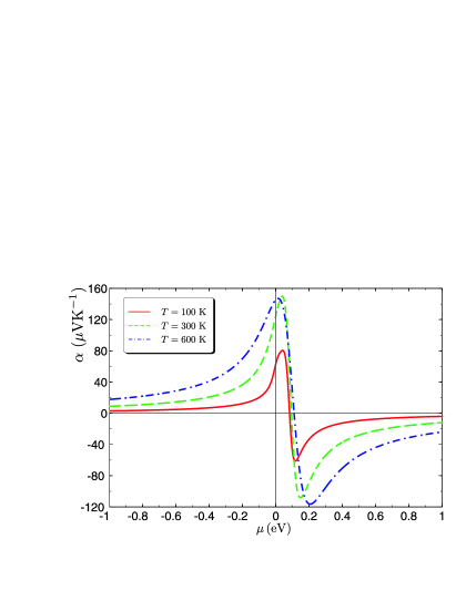
Figure 2: (Color online) Seebeck coefficient $\alpha$ of graphene as a function of chemical potential $\mu$ for indicated values of temperatures $T$.

The above described behavior of the thermocurrent and electrical resistivity is also reflected in the dependence of the Seebeck coefficient $\alpha$ on the chemical potential $\mu$, as shown in Fig. 2. To calculate $\alpha$, we used Eq. (7) and take the parameters $V_{0}/V_{c}=-100$ and $N_{i}=2\times 10^{14}$ m^-2, where $V_{c}=ta_{0}^{2}$, $t=3$ eV is the hopping integral and $a_{0}=1.42\times 10^{-10}$ m is the distance between carbon atoms in graphene. Obviously, the thermopower (Seebeck coefficient) is equal to zero at the chemical potentials where the thermocurrent vanishes. For larger chemical potentials, the thermopower is negative since the current is dominated by particles. In turn, for lower chemical potentials the thermopower is positive as the current is then dominated by holes. Interestingly, the maxima in the absolute magnitude of the thermopower appear at the points, where the change in resistance (and thus also in transmission through the graphene) with the chemical potential reaches a maximum.

Figure 3: (Color online) Figure of merit $ZT$ for graphene as a function of the chemical potential $\mu$ (a) and as function of temperature $T$ (b), for indicated values of the impurity potential $V_{0}$.

Figure 3 shows the corresponding figure of merit $ZT$, defined as

$$ZT=\frac{T\alpha^{2}\sigma}{\kappa},$$ (19)

as a function of the chemical potential, Fig. 3(a), and as a function of temperature, Fig. 3(b). The temperature dependence of $ZT$ in Fig. 3(b) is shown for the chemical potentials $\mu$, where the corresponding $ZT$ achieves a maximum in Fig. 3(a). Note, the figure of merit vanishes at the chemical potentials where the thermopower vanishes (maxima of the resistance). However, there is a significant enhancement of the figure of merit due to resonant scattering on impurities, and the enhancement appears at the chemical potential where the electrical resistance varies rapidly with $\mu$. However, one should bear in mind, that this figure of merit has been calculated taking into account the electronic term in the heat conductance only. A phonon contribution to the heat conductance inevitably suppresses $ZT$ to remarkably smaller values.

Figure 4: (Color online) The Wiedemann-Franz ratio as a function of chemical potential $\mu$ for $T=300$ K. The black line corresponds to the Lorentz number in metals, $L_{0}=2.44\times 10^{-8}\ {\rm W\Omega K^{-2}}$, whereas $L_{G}=5.79\times 10^{-8}$ W${\rm\Omega}$K^-2 corresponds to the Wiedemann-Franz ratio for graphene at $\mu=0$ and constant relaxation time.

V The Wiedemann-Franz law for graphene

Let us consider now the Wiedemann-Franz law. In ordinary metals this law states that the ratio $\kappa/\sigma T$ is constant,

$$\frac{\kappa}{T\sigma}=L\,,$$ (20)

where $L=L_{0}=\pi^{2}k_{B}^{2}/3e^{2}=2.44\times 10^{-8}\ {\rm W\Omega K}^{-2}$ is a constant, known as the Lorentz number. The situation in graphene is different. Strong energy dependence of the relaxation time and the presence of resonance states, lead to a significant dependence of the ratio $\kappa/\sigma T$ on the chemical potential $\mu$, as shown in Fig. 4 for $T=300$ K and indicated values of the scattering potential $V_{0}$. Experimentally, the chemical potential can be tuned by an external gate voltage. As one can see, this ratio is not constant, but strongly depends on the chemical potential $\mu$, especially in the vicinity of the resonance states. Moreover, this ratio also depends on the impurity potential $V_{0}$. However, far from the resonance states, when the Fermi level is well inside the upper (positive $\mu$) or lower (negative $\mu$) band, the ratio $\kappa/\sigma T$ tends to the number typical in metals, i.e. to $L_{0}$. It is rather clear, that the deviation of the ratio $\kappa/\sigma T$ from $L_{0}$ follows from the resonance states and specific electronic structure of graphene (energy dependent density of states). Similar deviations are also known in other systems, for instance in transport through nanoscopic quantum objects like quantum dots, molecules, etc.

It is interesting to consider the situation which may be directly compared to ordinary metals, i.e. when the relaxation time due to impurity scattering is constant $\tau=\tau_{0}$ in the vicinity of the point $\mu=0$. The corresponding ratio $L$ is shown in figure 4. When the chemical level is well inside the valence or conduction bands, $|\mu|>>0$, the ratio $\kappa/\sigma T$ tends to the Lorentz number $L_{0}$, as in the case of resonance states. However, this ratio has a maximum at $\mu=0$, i.e. at the point where the density of states in graphene disappears.

One can calculate the Wiedemann-Franz ratio of graphene at $\mu=0$ analytically assuming that the relaxation time is constant $\tau=\tau_{0}$ in the vicinity of the point $\mu=0$. In other words, we assume that one can neglect the dependence of $\tau$ on energy, $\delta\tau(\varepsilon)/\tau\ll 1$ for $|\varepsilon|\leq k_{B}T$, which is certainly fulfilled at rather low temperatures for any dependence $\tau(\varepsilon)$. In such a case, the kinetic coefficient $K_{21}=0$, and the other coefficients can be calculated analytically

$$K_{11}=\frac{\tau_{0}k_{B}T\ln 2}{2\pi\hbar^{2}}\,,$$ (21)

$$K_{31}=\frac{9\zeta(3)\tau_{0}k_{B}^{3}T^{3}}{4\pi\hbar^{2}}\,.$$ (22)

Using Eq.(21) and Eq.(22), one can calculate the Lorentz number for graphene at $\mu=0$,

$$L_{G}\equiv\left.\frac{\kappa}{\sigma T}\right|_{\mu=0}=\frac{9k_{B}^{2}\,\zeta(3)}{2e^{2}\ln 2}\,,$$ (23)

where $\zeta(x)$ is the Riemann’s $\zeta$-function. This value of $L_{G}$ is equal to $5.795070903\times 10^{-8}\,{\rm W\Omega K^{-2}}$. Taking into account that $L=\pi^{2}k_{B}^{2}/3e^{2}$ we can also find

$$\frac{L_{G}}{L}=\frac{27\,\zeta(3)}{2\pi^{2}\ln 2}\simeq 2.37.$$ (24)

This result was also obtained earlier by Saito et al.saito2007 for the case of purely ballistic electric and thermal conductance of graphene, when $\mu=0$.

VI Conclusions

We have analyzed theoretically the thermoelectric properties of graphene with impurities equally distributed in both A and B sublattices. These impurities lead to resonance impurity states near the Fermi level, and therefore to resonance electron scattering. In agrement with the Mott’s law, the magnitude of the Seebeck coefficient $\alpha$ and shape of its dependence on the chemical potential is strongly affected by the dependence of the conductivity on $\mu$, which in turn is determined mainly by the electron scattering from impurities in the vicinity of resonance states. The resonant states also lead to significant enhancement of the figure of merit $ZT$.

We have also shown that the ratio $\kappa/\sigma T$ deviates from the Lorentz number $L_{0}$, and this deviation appears for chemical potentials in the vicinity of the resonant states. Moreover, assuming a constant relaxation time we have found analytical solution for the ratio $\kappa/\sigma T$ at $\mu=0$, which agrees with that derived earlier.

In our calculations we introduced the impurity density $N_{i}$, the impurity scattering potential $V_{0}$, and the chemical potential $\mu$ as independent parameters. This assumption can be justified, if there are other (not necessarily resonant) impurities and defects in graphene. Additionally, the chemical potential can be tuned also by an external gate voltage, which gives an additional experimental tool to study the thermoelectric properties of graphene and their dependence on these parameters.

- (1) A. A. Balandin, S. Ghosh, W. Bao, I. Calizo, D. Teweldebrahn, F. Miao, and C. Lau, Nano Lett. 8, 902 (2008).
- (2) Y. Xu, Z. Li, and W. Duan, arXiv: 1401.3415v2 (2014).
- (3) D. Dragoman and M. Dragoman, Appl. Phys. Lett. 91, 203116 (2007).
- (4) T. Lofwander and M. Fogelstrom, Phys. Rev. B 76, 193401 (2007)
- (5) D. Wang and J. Shi, Phys. Rev. B 83, 113403 (2011).
- (6) Y. M. Zuev, W. Chang, and P. Kim, Phys. Rev. Lett. 102, 096807 (2009).
- (7) L. Zhu, R. Ma, Li Sheng, M. Liu, and D.-N. Sheng, arXiv: 0908.4302v2 (2010).
- (8) X. Z. Yan and C. S. Ting, Phys. Rev. B 83, 113403 (2011).
- (9) S. G. Sharapov and A. A. Varlamov, Phys. Rev. B, 86, 035430 (20012).
- (10) L. Hao and T. K. Lee, Phys. Rev. B, 82 245415 (2010).
- (11) M. Wierzbowska and A. Dominiak, G. Pizzi, arXiv:1403.1286v1 (2014).
- (12) M. Wierzbowska, A. Dominiak, arXiv:1403.4989v1 (2014).
- (13) Z. G. Fthenakis, Z. Zhu, and D. Tomanek, Phys. Rev. B, 89, 125421 (2014).
- (14) P. Wei, W. Bao, Y. Pu, C.N. Lau, and J. Shi, Phys. Rev. Lett. 102, 166808 (2009)
- (15) X. Ni, G. Liang, J.-S. Wang, and B. Li, Appl. Phys. Lett. 95, 192114 (2009)
- (16) T. Gunst, T. Markussen, A.-P. Jauho, and M. Brandbyge, Phys. Rev. B84, 155449 (2011).
- (17) H. Karamitaheri, M. Pourfath, R. Faez, and H. Kosina, J. Appl. Phys. 110, 054506 (2011).
- (18) Y. Yan, Q.-F. Liang, H. Zhao, C.-Q. Wu, and B. Li, Phys. Letters A 376, 2425 (2012).
- (19) P.-H. Chang and B. Nikolić, Phys. Rev. B 86, 041406(R) (2012).
- (20) M. Wierzbicki, R. Swirkowicz, and J. Barnaś, Phys. Rev. B 88, 235434 (2013).
- (21) C. L. Kane and E. J. Mele, Phys. Rev. Lett. 95 226801 (2005).
- (22) G. D. Mahan, Many Particle Physics, New York: Plenum (2009).
- (23) P. S. Kireev, Semiconductor Physics, (Mir Publishers, Moscow, 1974).
- (24) M. Inglot and V. K. Dugaev, J. Appl. Phys. 109, 123709 (2011).
- (25) K. Saito, J. Nakamura, and A. Natori, Phys. Rev. B 76, 115409 (2007).