A multiwavelength study of the hierarchical triple HD 181068:

HD 181068 is the only compact, triply eclipsing, hierarchical triple system containing a giant star known to date. With its central, highly-active G-type giant orbited by a close pair of main-sequence dwarfs, the system is ideal to study tidal interactions. We carried out a multiwavelength study to characterize the magnetic activity of the HD 181068 system. To this end, we obtained in- and out-of-eclipse X-ray snapshots with XMM-Newton and an optical spectrum, which we analyzed along with the Kepler light-curve. The primary giant shows strong quiescent X-ray emission at a level of $2\times 10^{31}$ erg s^-1, an S-index of $0.41\pm 0.01$, and marked white-light flares releasing up to $6\times 10^{38}$ erg in the Kepler-band. During the second X-ray observation, we found a three-times elevated – yet decaying – level of X-ray emission, which might be due to an X-ray flare. The high level of magnetic activity is compatible with the previously reported absence of solar-like oscillations in the giant, whose atmosphere, however, undergoes tidally-induced oscillations imposed by the changing configuration of the dwarf-binary. We found that the driving force exciting these oscillations is comparable to the disturbances produced by a typical hot Jupiter, making the system a potential test bed to study the effects of tidal interactions also present in planetary systems.

1 Introduction

While stellar triple systems are not at all rare, the systems HD 181068 and KOI-126 are the only compact triples with mutually eclipsing components currently known (Raghavan et al., 2010; Carter et al., 2011; Derekas et al., 2011). Of these two, only HD 181068 harbors an evolved giant star in its center. Due to the absence of an orbital equilibrium state, compact triple systems are ideal laboratories to study tidal interactions, orbital evolution, and to test models of stellar evolution (e.g., Fuller et al., 2013).

The central G-type giant of HD 181068 is orbited by a close pair of main-sequence dwarfs. While the dwarf-binary completes a full orbit around the giant in $45$ d, its components revolve around each other every $0.9$ d (see Table 1 and Borkovits et al., 2013). All mutual eclipses have been observed with high accuracy by the Kepler satellite (Derekas et al., 2011). Because the effective temperatures of the three system components are identical to within about $400$ K (see Table 1), the transit light-curves resulting from the eclipse of the giant by the dwarf-binary and vice versa do not differ substantially in depth. They can, however, be distinguished through their shape, because the primary transit light-curve, with the binary passing in front of the giant, yields a rounder profile resulting from limb darkening. The secondary eclipse, during which the dwarf binary is entirely occulted by the giant, shows a box-like profile (e.g., Derekas et al., 2011).

The duration of the phase of total eclipse in the AB system depends on the respective geometry. Borkovits et al. (2013) showed that the eclipse geometry essentially repeats after five orbits of the AB system, i.e., after about $227$ d. The total duration of every eclipse – primary or secondary – amounts to approximately $1.5$ dwarf-binary orbits or $\approx 1.35$ d in every case.

The HIPPARCOS-measured parallax of HD 181068 is $4.02\pm 0.4$ mas, resulting in a distance of $249\pm 25$ pc. Borkovits et al. (2013) derived a preliminary age estimate of $300-500$ Ma for the HD 181068 system by comparing the stellar parameters to evolutionary tracks. The authors caution, however, that the dwarf radii “appear to be significantly larger than expected”, and more sophisticated modeling may be necessary.

The structure of the HD 181068 system is reminiscent of that of RS Canum Venaticorum (RS CVn) systems – binary systems consisting of a G- or K-type giant orbited by a late-type main-sequence or subgiant companion (Dempsey et al., 1993a; Hall, 1976). RS CVn systems are among the most active stellar systems in the Galaxy as evidenced, among others, by pronounced and variable emission-line cores in Ca II H and K and H$\alpha$, starspots, photometric variability, and X-ray emission (e.g., Linsky, 1984; Strassmeier et al., 1988; Schmitt et al., 1990; Dempsey et al., 1993a). In RS CVn systems with periods shorter than about $30$ d, rotation and orbital motion are typically synchronized (Zahn, 1977; Scharlemann, 1982; Dempsey et al., 1993a; Derekas et al., 2011). In HD 181068, Derekas et al. (2011) derived a rotational velocity of $v\sin(i)=14$ km s^-1 for the giant, which, combined with its radius, suggests that the orbital period of the AB system and the giant’s rotation are also synchronized.

In a Fourier analysis of the Kepler light-curve, Borkovits et al. (2013) found substantial photometric variability at a period comparable to the AB system’s orbital period. The observed amplitudes exceed the expectation for ellipsoidal variation. Because the giant’s rotation is likely synchronized with the AB system’s orbital motion, this strongly suggests rotational modulation due to starspots, which might even be seen as distortions in some primary-eclipse light-curves (Borkovits et al., 2013, Fig. 5). The authors proceed to argue that their Fourier analysis reveals a double-peak close to the presumed rotation period of the giant, which may be a consequence of differential rotation.

Furthermore, the Kepler light-curve shows a highly interesting behavior at higher frequencies. First, it reveals a number of oscillation periods that can be attributed to tidal interactions between the changing configuration of the dwarf-binary and the atmosphere of the giant (Derekas et al., 2011; Borkovits et al., 2013; Fuller et al., 2013). Such tidally-induced oscillations can only be observed in sufficiently close systems such as HD 181068 or, potentially, planetary systems. Second, solar-like oscillations of the central giant are absent or strongly suppressed (Derekas et al., 2011; Fuller et al., 2013). Chaplin et al. (2011) argued that solar-like oscillations are damped by magnetic activity in solar-like stars; according to these authors, this certainly seems also to be the case in the Sun. Therefore, Fuller et al. (2013) speculate that strong activity may also suppress solar-like oscillations in the central giant HD 181068 A. Some support for this argument comes from a number of pronounced flare-like events observed in the Kepler light-curve, one of which is observed during a secondary eclipse (Borkovits et al., 2013, Fig. 6) and, thus, must be attributed to the giant, if it originates in the HD 181068 system. Another indication for a high level of magnetic activity has been contributed by the ROSAT all-sky survey, which revealed a clear X-ray source with a count rate of $0.294\pm 0.023$ ct s^-1 at the position of HD 181068, suggesting an X-ray luminosity on the order of $2\times 10^{31}$ erg s^-1 (cf., Sect. 2.4).

In this paper, we present a multiwavelength study of stellar activity in the HD 181068 system. In particular, we provide a detailed analysis of the X-ray emission from the HD 181068 system based on two carefully timed XMM-Newton observations, study the white-light flares observed in the Kepler light-curves, and investigate the chromospheric Ca II H and K emission using an optical spectrum obtained during secondary eclipse.

Table 1: Stellar properties of the system components (Borkovits et al., 2013).

	A	Ba	Bb
m [M⊙]	$3\pm 0.1$	$0.915\pm 0.034$	$0.870\pm 0.043$
R [R⊙]	$12.46\pm 0.15$	$0.865\pm 0.01$	$0.8\pm 0.02$
Teff [K]	$5100\pm 100$	$5100\pm 100$	$4675\pm 100$
Lbol [L⊙]	$92.8\pm 7.6$	$0.447\pm 0.037$	$0.27\pm 0.027$
$\log(g)$ [cgs]	$2.73$	$4.53$	$4.58$

Table 2: Orbital parameters of the HD 181068 system (Borkovits et al., 2013). Numbers in parentheses indicate error in last digits.

	A$-$B	Ba$-$Bb
T${}_{MIN,p}^{a}$ (BJDTDB)	$2\,455\,499.9970(4)$	$2\,455\,051.237\,00(5)$
P [d]	$45.4711(2)$	$0.9056768(2)$
a [R⊙]	$90.31\pm 0.72$	$4.777\pm 0.039$
i [∘]	$87.5\pm 0.2$	$86.7\pm 1.4$

Table 3: Duration (DUR.) and sum of “good time intervals” (ONTIME) for the individual instruments of our XMM-Newton observations.

	0722330201		0722330301
	DUR.a	ONTIME	DUR.a	ONTIME
Instr.	[ks]	[ks]	[ks]	[ks]
pn	13.0	11.7	12.0	8.2
MOS 1	14.6	14.5	13.6	13.6
MOS 2	14.6	14.6	13.6	13.6

2 X-ray observations and data analysis

We observed HD 181068 twice using XMM-Newton. While the first X-ray observation was carried out when both giant and dwarf-binary component were visible, the second observation had been scheduled during secondary eclipse, when the dwarf-binary remained hidden behind the giant. The timing details are given in Table 4, where the phase is defined as a value between zero and one according to the ephemeres given in Table 1. In both observations, we used the medium filter for pn and MOS 1 and the thick filter for MOS 2.

Table 4: Timing of the XMM-Newton observations.

	UTCa	JD${}_{UTC}^{b}$	BJD${}_{TDB}^{b}$
Observation ID 0722330201
Start	2013-05-03 4:26	$415.684\,72$	$415.685\,98$
End	2013-05-03 8:03	$415.835\,42$	$415.836\,68$
Phase	$0.1378-0.1411^{c}$
Observation ID 0722330301
Start	2013-05-19 14:56	$432.115\,28$	$432.117\,24$
End	2013-05-19 18:17	$432.261\,81$	$432.263\,78$
Phase	$0.4992-0.5024^{c}$

We reduced the data using XMM-Newton’s “Scientific Analysis System” (SAS) in version 12.0.1 applying standard recipes and filtering recommendations. The duration of the observations and the available time remaining after the filtering are given in Table 3. While the pn-exposure during the in-eclipse phase (ID 0722330301) suffers from high background toward the end of the observation, the MOS instruments remain virtually unaffected. The X-ray data analysis was carried out using XSPEC in version 12.5.0 (Arnaud, 1996).

An X-ray source at the position of HD 181068 is evident in both the in- and out-of-eclipse X-ray images. Figure 1 shows the in-eclipse X-ray image of HD 181068 observed by the pn-camera. In this phase, we even found a stronger source with a count rate approximately tripled compared to the previous out-of-eclipse exposure (Table 6).

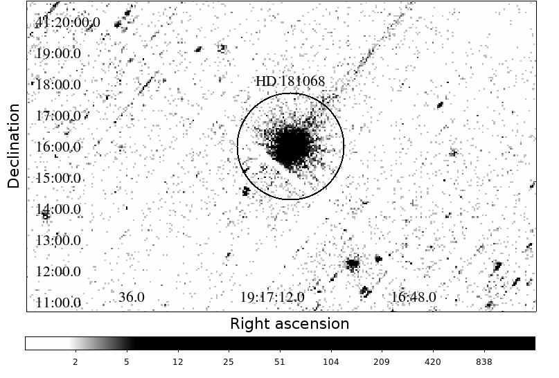
Figure 1: In-eclipse X-ray image of HD 181068 (pn).

2.1 Short-term X-ray variability

To check for short-term X-ray variability in HD 181068, we constructed $0.3-6$ keV light-curves using the evselect and epiclccorr routines. The latter corrects for various effects such as vignetting, bad pixels, good-time intervals, and dead time. As an example, we show in Fig. 2 the MOS 1 light-curve observed during May 3 and 19.

First, we fitted the MOS 1, MOS 2, and pn light-curves using a constant model. The resulting best-fit count-rates are listed in Table 5. Second, we fitted a linear model. While the constant could be varied independently for the three instruments, the gradient was taken to be identical for all simultaneous light curves. In Table 5 the $\chi^{2}$-values and number of degrees of freedom (dof) for the best-fit constant and linear model are listed. Applying an F-test, we found that the model including the linear term provides a better description of the data at the $95$% confidence level in both cases. In particular, we find p-values of $0.02$ and $10^{-16}$ for May 3 and 19.

The lower level and relative stability of the X-ray count-rate on May 3 suggest to identify the X-ray flux observed then with the quiescent X-ray emission level; this interpretation is also consistent with the ROSAT observation, which yields a similar flux (cf., Sect. 2.4). On May 19, we did not only find a higher X-ray luminosity but also a more strongly declining X-ray count-rate, which seems less typical for quiescent emission.

During both X-ray observations, XMM-Newton’s Optical Monitor (OM) observed HD 181068 with the UVM2 filter in imaging mode. Comparing the images, we derived a decrease of $0.36\pm 0.27$% in the OM count-rate during the eclipse. This is roughly compatible with an expected $0.8$%, assuming that the luminosities of the system components in the UVM2 filter are proportional to their bolometric luminosities. The OM provides no evidence for an increased near ultra-violet count-rate accompanying the elevated X-ray count-rate during the in-eclipse observation.

Table 5: Fit results for the constant and linear model along with the best-fit $\chi^{2}$-values and the number of degrees of freedom (dof).

Instrument	CRa May 3	CRa May 19
	[ct $s^{-1}$]	[ct $s^{-1}$]
	Best-fit constants
pn	$1.45\pm 0.013$	$3.374\pm 0.025$
MOS 1	$0.387\pm 0.006$	$0.938\pm 0.009$
MOS 2	$0.325\pm 0.005$	$0.828\pm 0.009$
	Best-fit gradient [ct s-1 ks-1]
Combined	$-0.0023\pm 0.0009$	$-0.0125\pm 0.0015$
$\chi^{2}$-values and dof
Constant	239.1/207	232.9/206
Linear	200.8/179	136.8/178

Figure 2: Background-subtracted MOS 1 light-curve of HD 181068 in the $0.3-6$ keV band with $200$ s binning.

2.2 Spectral analysis of pn and MOS data

Figure 3: Merged, in-eclipse RGS 1+2 spectrum of HD 181068 with 15 counts per spectral bin. Labels denote the most prominent spectral lines.

The pn count-rate of HD 181068 is sufficiently high to produce a source with substantial signal exceeding the background level even in the wings of the point-spread-function (PSF). Therefore, we opted for a $30^{\prime\prime}$-radius source region to take full advantage of the high flux in our analysis. Strong X-ray sources are susceptible to pile-up, due to the limited detector read-out cadence. The “XMM-Newton users’ Handbook” (Sect. 3.3.2, Table 3) states critical limits of $8$ ct s^-1 for the pn and $0.7$ ct s^-1 for the MOS instruments operated in “full frame” mode, beyond which pile-up starts to seriously deteriorate the X-ray spectra. According to these limits, pile-up is no issue for the pn data; the MOS data may be mildly affected (cf., Table 5). An additional analysis of the pn-data based on the SAS-tool epaplot also yielded a negligible pile-up fraction. As we further see no difference between the MOS data observed with the thick and medium filter, we consider pile-up and optical loading irrelevant in our analysis.

Table 6: Best-fit parameters based on pn and MOS data and the RGS data with $90$% confidence intervals.

pn and MOS
	May 3	May 19
NH [$10^{22}$ cm-2]	$0.021_{-0.004}^{+0.004}$	$0.044_{-0.004}^{+0.004}$
T1 [keV]	$0.92_{-0.04}^{+0.04}$	$0.88_{-0.05}^{+0.07}$
EM${}_{1}^{a}$ [$10^{53}$ cm-3]	$7.5_{-0.3}^{+0.3}$	$7.7_{-0.5}^{+0.5}$
T2 [keV]	$1.88_{-0.11}^{+0.12}$	$1.95_{-0.24}^{+0.48}$
EM${}_{2}^{a}$ [$10^{53}$ cm-3]	$10.4_{-0.4}^{+0.4}$	$28.6_{-1.3}^{+1.3}$
T3 [keV]		$8.6_{-2.2}^{+37}$
EM${}_{3}^{a}$ [$10^{53}$ cm-3]		$12.8_{-0.8}^{+0.8}$
Ab.Fe,Mg,Al,Ni,Ca [$\odot$]	$0.23_{-0.03}^{+0.02}$
Ab.C,N,O,S,Si [$\odot$]	$0.16_{-0.05}^{+0.05}$
Ab.Ne,Ar [$\odot$]	$0.73_{-0.21}^{+0.21}$
$\log_{10}(\mbox{Flux [cgs]})^{a,b}$	$-11.5896_{-0.008}^{+0.008}$	$-11.0877_{-0.006}^{+0.006}$
$\chi^{2}$/dof	$1729.5/1631$
RGS
Ab.Fe,Mg,Al,Ni,Ca [$\odot$]	$0.35_{-0.09}^{+0.11}$
Ab.C,N,O,S,Si [$\odot$]	$0.55_{-0.14}^{+0.19}$
Ab.Ne,Ar [$\odot$]	$1.49_{-0.38}^{+0.49}$

In our spectral analysis, the spectra were modeled with an absorbed thermal model with variable abundances (vapec, Smith et al., 2001). In particular, we used two temperature components for the May 3 observation and included an additional hot component for the observation on May 19. This model is motivated by the results of more detailed grating observations of the RS CVn systems II Peg and AR Lac (Huenemoerder et al., 2001, 2003). While these systems show complex differential emission measure (DEM) distributions, the DEM reconstructions also show distinct peaks. In the case of AR Lac the DEM peaks at about $0.1$ keV, $0.69$ keV, and $1.9$ keV. In both cases, the low-temperature end of the DEM remains mostly constant in time, while variability manifests at the high-temperature end of the DEM. In the particular case of II Peg, a flare was observed, which could be modeled as an addition of a hot component to the DEM without affecting the cooler components (Huenemoerder et al., 2001).

We treated both observations and the MOS and pn instruments simultaneously in our spectral analysis. The pn and MOS spectra were grouped into bins comprising $15$ counts each, which renders the $\chi^{2}$-statistic applicable. In our treatment of the elemental abundances, we followed the approach of Schmitt & Robrade (2007) and grouped the elements with respect to their first ionization potential (FIP). In particular, low-FIP (Fe, Mg, Al, Ni, Ca; FIP$<8$ eV), medium-FIP (C, N, O, S, Si; $8$ eV $<$ FIP $<15$ eV), and high-FIP elements (Ne, Ar; FIP $>15$ eV) were distinguished; solar abundances refer to those given by Anders & Grevesse (1989).

While the abundance pattern was coupled among all thermal components in the fit, their temperatures and emission measures could be varied independently. The sum of the thermal components was subject to absorption represented by the phabs model, and a different depth of the absorption column was allowed for the two observations. To compute the unabsorbed flux and its error, we applied the cflux model. Please note that the values and errors of the emission measures were calculated with the cflux component removed and all other parameters fixed to ensure consistency; the errors may, therefore, be slightly underestimated. With this approach we obtained a model with a reduced $\chi^{2}$ value of $1.06$; our results are summarized in Table 6.

While the lowest-temperature component characterized by $T_{1}$ and EM₁ remained virtually unchanged between May 3 and May 19, the medium-temperature component approximately tripled its emission measure, EM₂, but remained at about the same temperature. For the temperature of the third, hot component, $T_{3}$, we found a best-fit value of $100$ MK, which remained loosely determined, however. Demanding a common absorption column depth during both observations resulted in a model with reduced $\chi^{2}$ value of $1.12$, a column depth of $3.8\times 10^{22}$ cm^-2, and otherwise similar parameters. Formally, this solution provides an inferior model, which may indicate the presence of circumstellar material. However, this interpretation is not unique, because the corona of the giant also changed and the geometrical configuration during the two observations was different. The dwarf components are probably also highly active and provided an unknown and not explicitly accounted for coronal contribution only to the out-of-eclipse observation.

The fluxes given in Table 6 correspond to average X-ray luminosities of $(1.9\pm 0.4)\times 10^{31}$ erg s^-1 on May 3 and $(6.1\pm 1.2)\times 10^{31}$ erg s^-1 on May 19.

As we found evolution in the X-ray count-rate of HD 181068 during the observation on May 19, we also searched for temporal variability in the spectrum. In a first step, we examined a hardness ratio. In particular, we defined a low-energy band, $L$, ranging from $0.3-1$ keV and a high-energy band, $H$, from $1$ keV to $6$ keV, and the associated hardness ratio $HR=(H-L)/(H+L)$. Based on the MOS data, we found a mean hardness ratio of $0.62$. Applying a linear fit, we detected a decrease of $10^{-2}$ ks^-1 in hardness ratio, which is significant on the $99$% confidence level according to an F-test and is consistent with a softening of the X-ray spectrum. The pn data are also consistent with a decrease in hardness, but do not provide a significant result alone, because they do not offer the same temporal coverage. Further, the hardness ratio cannot be directly compared, because the spectral sensitivity of the pn is different. In a second step, we checked whether the decrease in hardness can directly be detected in a spectral analysis. To this end, we divided the observation into three $4.5$ ks chunks and repeated the previously described spectral analysis using the events pertaining to the individual observing chunks. We re-fitted the spectral model allowing, however, only the emission measure of the medium- and high-temperature components, EM₂ and EM₃, to vary. The remaining parameters remained fixed at the values reported in Table 6. We note that the temperature, $T_{3}$, of the high-temperature component was not well defined in any of the chunks. Applying a linear fit, we found an average decrease of $-1.9\times 10^{52}$ cm^-3 ks^-1 for EM₂ and $-4.1\times 10^{52}$ cm^-3 ks^-1 for EM₃, which is compatible with cooling of the high-temperature plasma component.

2.3 RGS data

In our analysis of the RGS data, we used the same spectral model as for the pn and MOS data (see 2.2), but focused on the abundances to which the RGS data are most sensitive. Their temperatures and absorption column depths were fixed to the values derived from the fits to the pn and MOS spectra, which cover a wider spectral range. The normalizations (i.e., emission measures) were left as free parameters to compensate for potential uncertainties in the cross-calibration.

To fit the RGS data, we grouped them into bins comprising 10 channels, resulting in an equally-spaced wavelength axis at the cost of leaving the $\chi^{2}$-statistic inapplicable. Therefore, we reverted to XSPEC’s W-statistic – applied when c-stat is used with Poisson-distributed background –, which does not rely on approximately Gaussian count distributions in the bins. Figure 3 shows the merged RGS $1+2$ spectrum of HD 181068 observed on May 19, grouped at 15 counts per bin for better visibility. The most prominent spectral feature is the Lyman-$\alpha$ line of O VIII  at about $19$ Å; further lines of Ne X, O VIII, and likely Fe XVII are clearly distinguished (see Fig. 3). The remaining structure is mostly due to emission of highly ionized iron ions – mainly Fe XVIII and Fe XIX. The data from RGS 1 and 2 as well as both spectral orders were fitted simultaneously, and the results are shown in Table 6.

While our fits to the RGS data yielded higher abundances than those obtained from the MOS and pn cameras, the trend for high-FIP elements to show higher abundance values is well reproduced. We note that the abundances of C, N, and O may be modified in the giant due to dredge-up of nucleosynthesis products from the stellar interior. Following the first dredge-up, for instance, a rise in the nitrogen surface abundance accompanied by a decrease in the carbon abundance is expected (Iben & Renzini, 1983). There is, however, no clear sign of such a pattern in our data.

2.4 ROSAT data and long-term variability

An X-ray source with a count rate of $0.294\pm 0.023$ ct s^-1 at the position of HD 181068 has also been detected by ROSAT. Assuming an interstellar absorption column of $3\times 10^{20}$ cm^-2 and a mean coronal temperature between $1$ and $1.5$ keV, we converted the ROSAT count-rate into unabsorbed $0.3-9$ keV fluxes, $\log_{10}(\mbox{Flux [cgs]})$, between $-11.5$ and $-11.36$, corresponding to X-ray luminosities between $2.3$ and $4\times 10^{31}$ erg s^-1. These estimates are compatible with the flux measurements by XMM-Newton and suggest that the X-ray luminosity of the HD 181068 system does not undergo strong variations on the timescale of decades.

3 Flares in the Kepler light-curve

The Kepler telescope observed HD 181068 uninterruptedly for almost four years from Quarter 1 through 16 (e.g., Koch et al., 2010). While only long-cadence data with about $30$ min sampling have been taken during the first six quarters, short cadence data, sampled at a temporal cadence of about one minute, become available for subsequent quarters. The Kepler light-curve of HD 181068 shows a wealth of intriguing features including marked transits caused by mutual eclipses of the giant and the dwarf-binary, transits in the dwarf-binary system, oscillations on the giant, ellipsoidal variations, rotational modulation, and flares; a detailed analysis of many of these features can be found in Derekas et al. (2011) and Borkovits et al. (2013).

In our analysis, we concentrated on the short-cadence data, which we obtained from the Kepler archive. We decided to use the Simple Aperture Photometry (SAP) and removed all data points flagged by the SAP_QUALITY column. To search for flares, we visually inspected the resulting light-curve, and thus identified seven clear flares, whose continuum-normalized light-curves are shown in Figs. 4 and 5. We note the apparent dip in brightness preceding some flares is not physical but rather caused by the normalization and the rather curved continuum. Although there are several smaller features in the light-curve that may also be flares, we found it impossible to verify their true nature, because the system’s optical light-curve is intrinsically strongly variable, and there may be additional instrumental effects. Therefore, we restrained our analysis to the seven evident flare events.

Although Derekas et al. (2011) and Borkovits et al. (2013) did not explicitly investigate the flares, one particularly interesting example has already been depicted by Borkovits et al.. This flare – shown in Fig. 4 – occurs during the secondary eclipse in the AB system, i.e., with the dwarf-binary hidden behind the giant. It can, therefore, uniquely be ascribed to the primary giant component.

To estimate the flare energy, we applied a continuum normalization to the individual flares. In particular, we defined the start and end point of the flares by visual inspection and fitted a first order polynomial to the flanking parts of the light curve. The flare light-curves shown in Fig. 5 were normalized by the thus obtained polynomial before subtracting unity. In the case of the flare occurring during secondary eclipse (see Fig. 4), we also modeled the transit shape based on the average secondary-transit profile of the AB system (Mandel & Agol, 2002). After dividing by the mean profile, we performed the same continuum normalization as for the other flares.

In Table 7, we give the time of the flare maximum, T_peak, the fractional increase in flux at flare maximum, f_peak, the duration of the rise- and decay-phase, t_rise and t_decay, and the total flare energy released in the Kepler band. We defined the duration of the rise phase as the estimated time of its start to the time of flux maximum. Equivalently, the decay phase lasts from the point of flux maximum to the estimated end of the flare. Because it is difficult to clearly distinguish flare-induced variability in the light curve, we estimated an uncertainty of about $10$ min for these numbers. The released energy, E_flare, was measured by integrating the flare light-curve and multiplying the result by the giant’s bolometric luminosity (see Table 1). Here, we implicitly assumed that the stellar and the flare spectrum are identical. Taking into account Kepler’s sensitivity curve (Van Cleve & Caldwell, 2009) and assuming black-body spectra with a temperature of $10\,000$ K for the flare and $5100$ K for the star, we found that the estimates would increase by about $30$%, which gives an idea of the systematic uncertainties involved in the calculation.

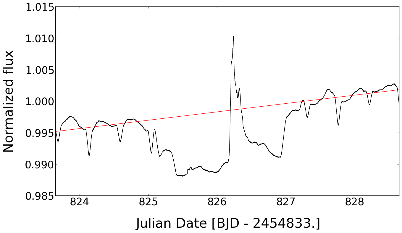
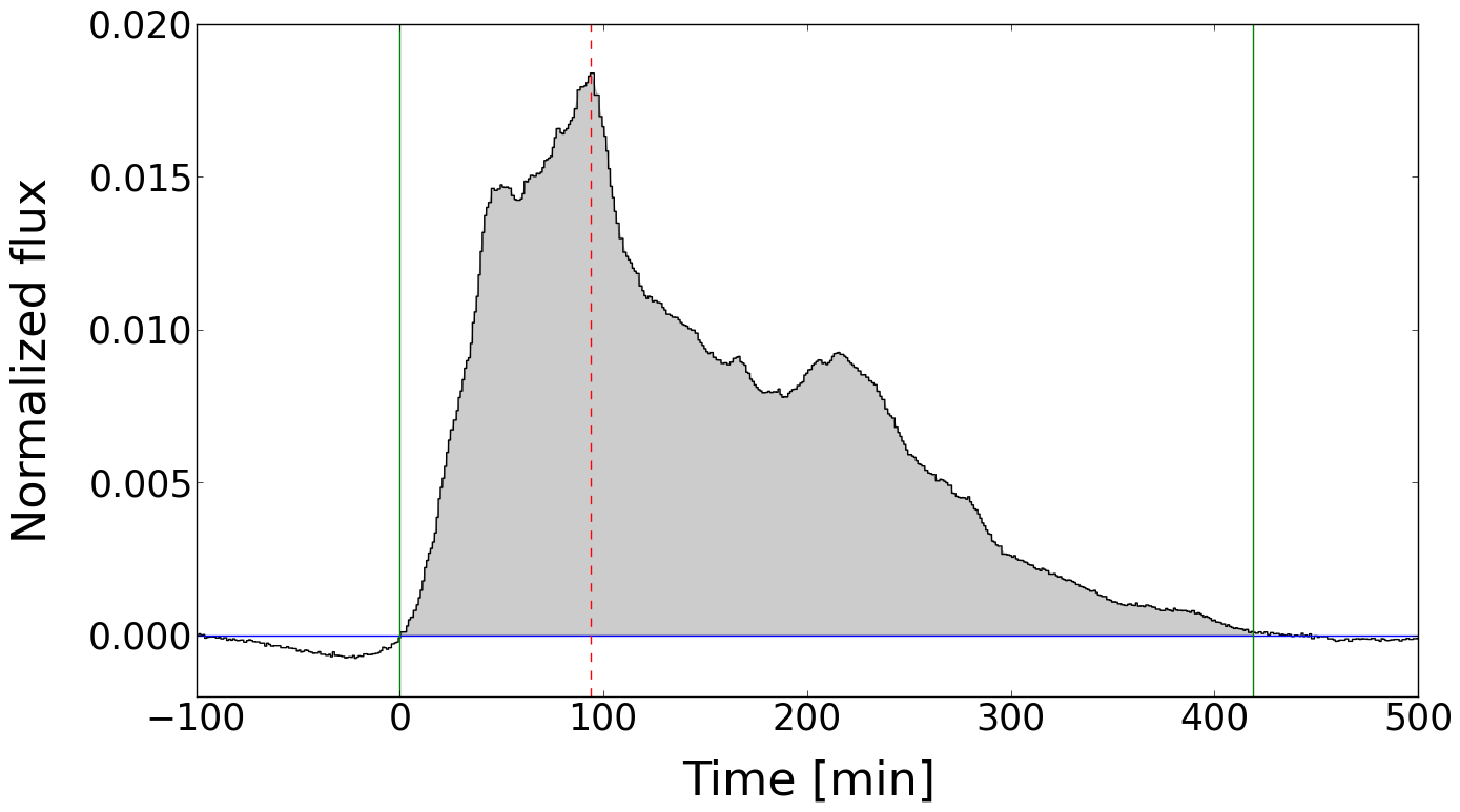
Figure 4: White-light flare observed during secondary eclipse (first flare listed in Table 7). Upper panel: Kepler light-curve of the secondary eclipse covering the flare. The red line shows the continuum normalization of the transit. Lower panel: Normalized flare light-curve. Vertical solid (green) lines indicate the start and end of the flare and the dashed (red) line marks the time of maximum flux.

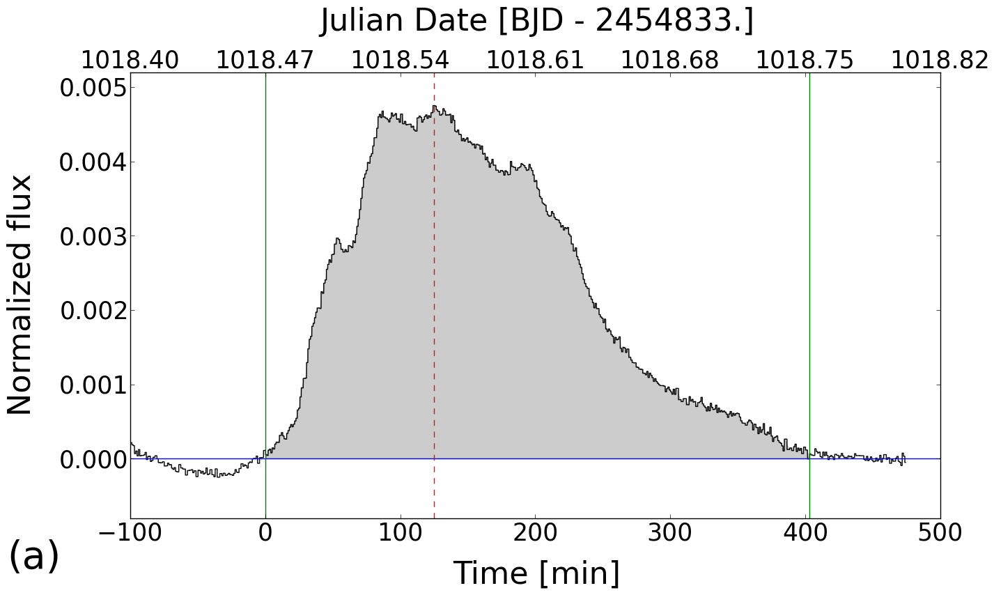
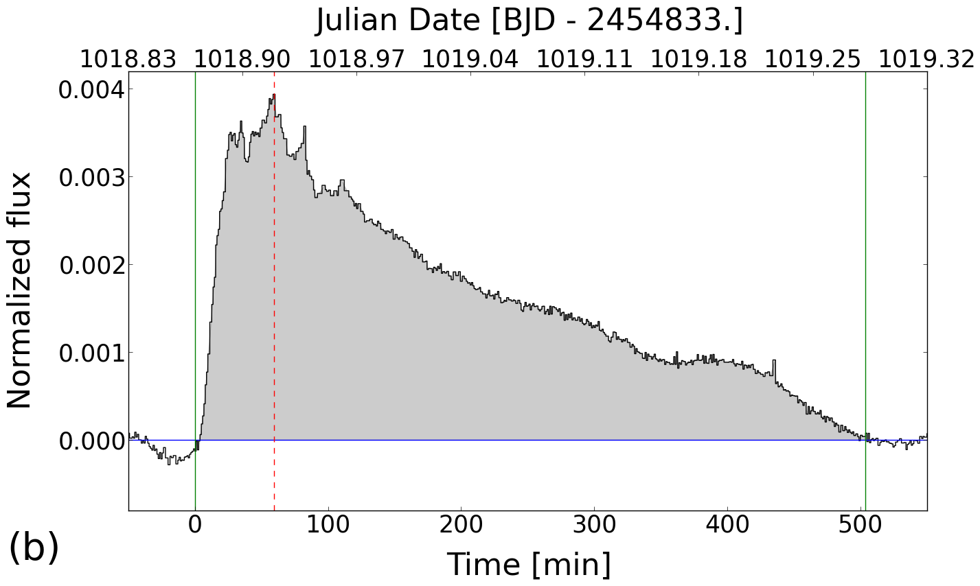
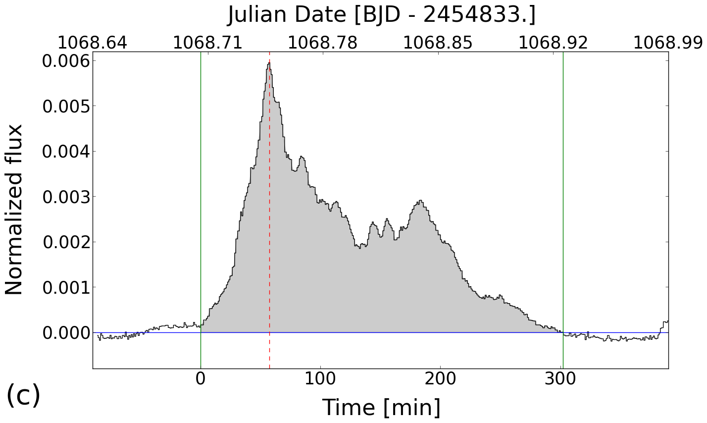
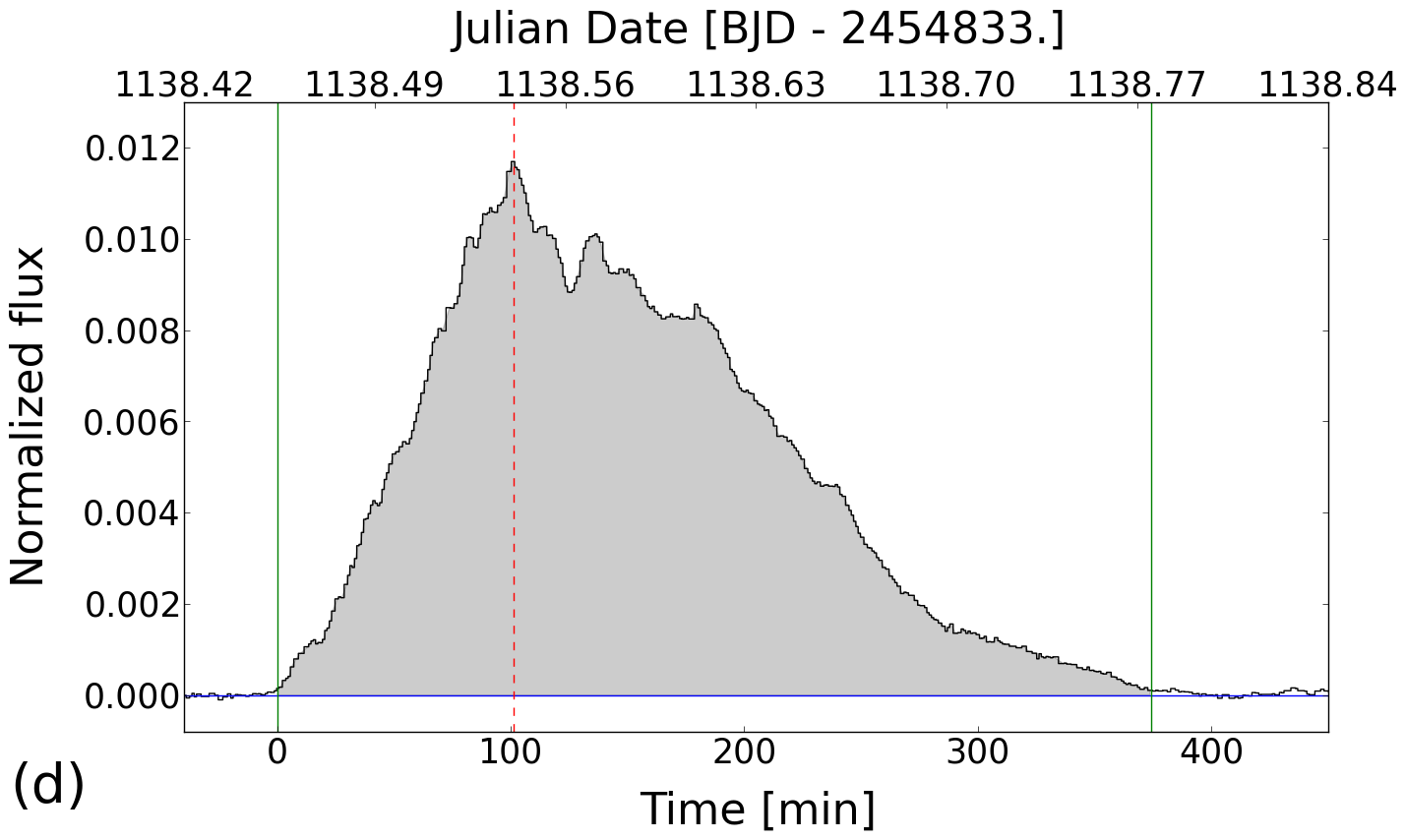
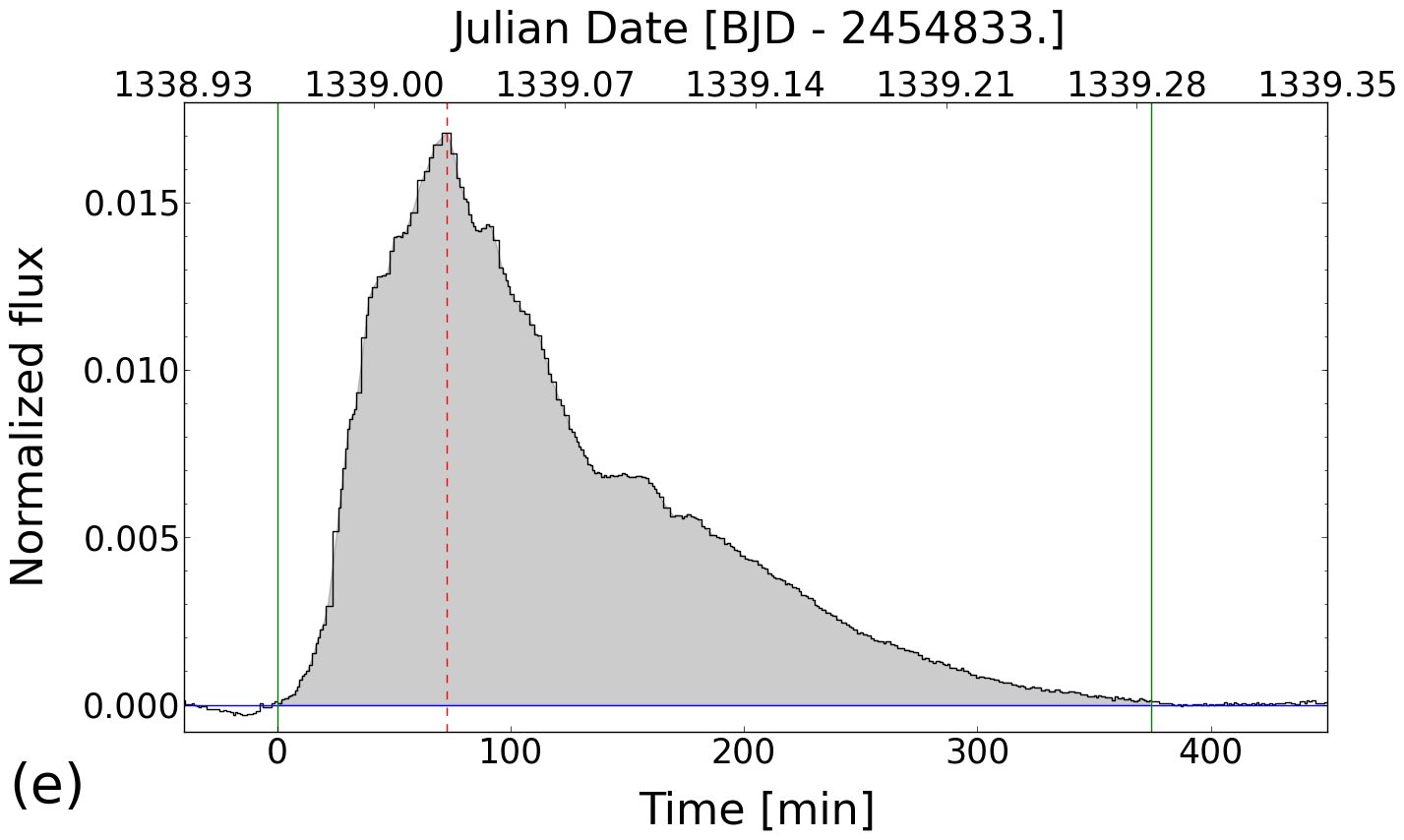
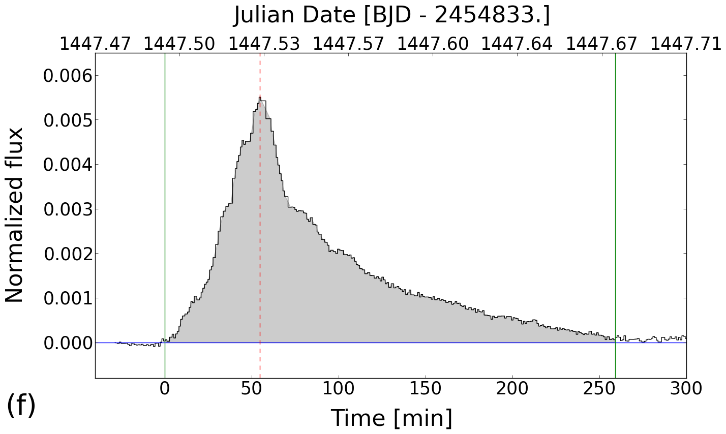
Figure 5: White-light flares observed by Kepler. The solid (green) lines indicate the start and end of the flares and the dashed (red) line the point of maximum flux.

Table 7: Properties of the seven flares found in the Kepler short-cadence light-curve of HD 181068.

T${}^{a}_{\mathrm{peak}}$	f${}^{b}_{\mathrm{peak}}$	t${}^{c}_{\mathrm{rise}}$	t${}^{c}_{\mathrm{decay}}$	E${}^{d}_{\mathrm{flare}}$
$[$d$]$	[%]	[min]	[min]	[erg]
$826.238$	$1.84$	$94$	$364$	$6\cdot 10^{38}$
$1018.557$	$0.48$	$125$	$278$	$2\cdot 10^{38}$
$1018.941$	$0.39$	$59$	$445$	$2\cdot 10^{38}$
$1068.750$	$0.60$	$57$	$245$	$1\cdot 10^{38}$
$1138.560$	$1.17$	$101$	$273$	$4\cdot 10^{38}$
$1339.051$	$1.71$	$73$	$302$	$4\cdot 10^{38}$
$1447.538$	$0.55$	$55$	$204$	$8\cdot 10^{37}$

3.1 Third-light origin of the flares?

Along with the reduced light-curves, the Kepler data archive provides pixel-scale data with a spatial resolution of about $4$ arcsec per pixel. Pixel-center shifts can be used to identify brightness variations not associated with the source under consideration, but originating on some unrelated back- or foreground object (Batalha et al., 2010).

To check the source position, the Kepler pipeline provides “moment-derived column and row centroids” (MOM_CENTR1/2) along with a correction based on reference stars (POS_CORR1/2). In the case of HD 181068, we found pixel-shifts, which are essentially proportional to the flux. With about $7$ Kepler magnitudes, HD 181068 is a particularly bright source suffering from charge bleeding and, therefore, has been assigned a large aperture elongated in the direction of the bleeding. Our analysis showed that this is also the direction in which the pixel-shifts are most pronounced, and we conclude that the observed shifts are most likely due to the characteristics of charge bleeding. In particular, we found no evidence for the flares being due to a third light source.

4 Ca II H and K observations of HD 181068

On Oct. 3, 2013, we carried out a $30$ min observation of HD 181068 using the “Telescopio Internacional de Guanajuato, Robótico-Espectroscópico” (TIGRE) – a $1.2$ m telescope located at La Luz, Mexico ($21^{\circ}$ N, $259^{\circ}$ E) (Schmitt et al., 2014). The telescope is equipped with the “Heidelberg Extended Range Optical Spectrograph” (HEROS), a fiber-fed, two-armed instrument, which provides spectral coverage from $3800-8800$ Å at a resolution of about $20\,000$.

The exposure was scheduled during secondary eclipse, so that only the giant’s spectrum has been observed. Figure 6 shows the Ca ii H and K lines with pronounced chromospheric fill-in, which has already been noticed by Derekas et al. (2011), who used the width of the emission cores to estimate the stellar absolute brightness via the Wilson-Bappu effect. From our spectrum, we derived a Mount-Wilson S-index of $0.41\pm 0.02$.

Using the relations given by Noyes et al. (1984) and the color-dependent conversion factor ($C_{cf}$) given by Rutten (1984), we converted the S-index into a $\log(R^{\prime}_{HK})$ value of $-4.57\pm 0.01$. Note that the conversion between Mount-Wilson S-index and $\log(R^{\prime}_{HK})$ has been revisited by a number of authors such as Hall et al. (2007) and Mittag et al. (2013), who obtained results differing by up to a factor of about two; see Hall et al. (2007) for a discussion of the development. For instance, using the calibration of the “arbitrary units” provided by Hall et al. (2007), we arrive at $\log(R^{\prime}_{HK})$ ratio of $-4.41$, which gives an impression of the systematic uncertainty involved in the conversion.

Figure 6: Ca II  H and K lines of HD 181068 A observed by TIGRE.

Its chromospheric emission puts HD 181068 A among the active giants with a chromosphere clearly emitting Ca ii H and K emission-line cores in excess of the basal level, which corresponds to an S-index value of $\lesssim 0.15$ for a G-type giant (Duncan et al., 1991; Schröder et al., 2012, Fig. 3). Figure 7 shows the $\log(R^{\prime}_{HK})$ index of HD 181068 in comparison to measurements of main-sequence and (sub-)giant stars presented by Strassmeier et al. (2000). Independent of the details of the calibration, HD 181068 qualifies as an active, albeit not an outstandingly active, giant star. We caution, however, that a single observation provides only a snapshot of the chromospheric properties.

Figure 7: The $\log(R^{\prime}_{HK})$ index of HD 181068 (filled circles) with the calibration of Noyes et al. (1984) and Hall et al. (2007) in comparison to the indices measured in the sample presented by Strassmeier et al. (2000); pluses denote main-sequence stars and squares subgiants and giants.

5 Discussion

5.1 Origin of the X-ray emission

Our detection of strong X-ray emission from HD 181068 during both the in- and out-of-eclipse phase suggests that the bulk of X-ray emission originates on the giant primary component. With the observed X-ray luminosity being even higher when the dwarf-binary was eclipsed, it remained impossible to directly identify the contribution of the dwarfs to the overall X-ray flux.

To estimate the dwarf-binary’s contribution to the total X-ray luminosity, we assumed coronal emission at the saturation limit of $L_{X}/L_{bol}=10^{-3}$, which has also been observed in other fast-rotating low-mass binaries such as YY Gem (Tsikoudi & Kellett, 2000; Stelzer et al., 2002; Pizzolato et al., 2003). Considering a total bolometric luminosity of $0.72$ L_⊙ for the dwarf-binary in HD 181068, we estimated an upper limit of $2.8\times 10^{30}$ erg s^-1 for their X-ray luminosity. Consequently, the dwarf-binary could contribute up to $15$% of the quiescent X-ray flux of the HD 181068 system. Because this contribution cannot be specified any further and the giant provides at least $85$% of the X-ray flux, we attribute the entire X-ray emission to the giant during the remaining analysis.

5.2 HD 181068 as an RS CVn system

RS CVn systems are among the strongest coronal X-ray sources in the Galaxy. Compared to single late-type giants in the solar neighborhood (Huensch et al., 1996), the X-ray luminosity of HD 181068 is elevated by about two orders of magnitude. Dempsey et al. (1993a) and Dempsey et al. (1993b) studied the X-ray emission of RS CVn systems based on ROSAT data. In their analysis of the coronal temperature, Dempsey et al. (1993b) found a bimodal distribution with peaks around $2\times 10^{6}$ K and $1.6\times 10^{7}$ K. Although we determined higher temperatures in the quiescent phase of HD 181068 (i.e., the May 3 observation), we also found satisfactory fits based on a two-temperature model in our analysis. This model certainly remains an approximation to the true distribution of emission measure in HD 181068, given that studies of the differential emission measure (DEM) in other RS CVn systems based on grating spectroscopy have revealed a continuous distribution of the emitting plasma (see Huenemoerder et al., 2001; Drake et al., 2001; Huenemoerder et al., 2003). However, the reconstructed DEMs also show distinct peaks (Huenemoerder et al., 2003, Fig. 5), so that a two-component approximation could, indeed, coarsely characterize the DEM. Attributing the observed X-ray emission to the giant, we estimated a quiescent surface X-ray flux, $F_{X}$, of $2\times 10^{6}$ erg cm^-2 s^-1. The resulting ratio of $0.57$ of Ca II H and K line surface-flux (Sect. 4) to $F_{X}$ is compatible with the values observed in the sample of young solar analogs presented by Gaidos et al. (2000) or the sample of giants shown by Pallavicini et al. (1982).

With its quiescent X-ray properties, we found that HD 181068 fits nicely into the sample presented by Dempsey et al. (1993a, Figs. 3 and 4). Assuming synchronous rotation of the giant and the AB system, we found that HD 181068 does neither show an outstanding X-ray luminosity nor surface X-ray flux. Also the relation between stellar radius and rotation period observed in HD 181068 does not set it apart from the sources reported by Dempsey et al. (1993a). Finally, we used the method presented by Eggleton (1983) to compute a value of $0.4$ for the giant’s Roche-lobe filling factor, $R_{s}/R_{lobe}$, and compared it with its X-ray luminosity and surface X-ray flux; in both cases, the result is compatible with the sample properties presented by Dempsey et al. (1993a) (see their Fig. 5).

Dempsey et al. (1993a) concluded that “other than acting to tidally spin up the system, the secondary plays no direct role in determining the X-ray activity level.” While the oscillation spectrum of HD 181068 A does clearly show that there is an interaction between the orbiting dwarf-binary and the giant’s atmosphere, this conclusion is not otherwise challenged by our X-ray observations of HD 181068.

5.3 Coronal abundances and first-ionization-potential effect

Derekas et al. (2011) determined a subsolar photospheric metallicity for HD 181068. Depending on the applied method, the authors state values of $[M/H]=-0.6\pm 0.3$ and $[M/H]=-0.2\pm 0.1$. These numbers are compatible with the mean coronal abundance for the low- and medium-FIP elements, which amounts to about $0.3$ times its solar equivalent corresponding to $[X/H]\approx-0.5$ for the respective element $X$ (Table 6).

The coronal abundance of the high-FIP elements is approximately solar, making them about three times overabundant with respect to the low- and medium-FIP elements. Assuming an overall solar photospheric abundance pattern in HD 181068, the abundance distribution is characteristic of an “inverse first ionization-potential” (IFIP) effect. While the IFIP effect is typically observed in the coronae of active stars (e.g., Brinkman et al., 2001; Drake et al., 2001; Telleschi et al., 2005), inactive stars tend to show a solar-like FIP-effect. The coronal abundances of HD 181068, therefore, indicate an active star.

5.4 White-light and X-ray flares

We analyzed seven flares observed by Kepler. Some of the flares show profiles indicative of multiple flare events (e.g., Figs 4 and 5 c), which may result from the eruption of a cascade of magnetic loops. In the following, we discuss their origin in the HD 181068 system, their energetics, and potential impact on coronal heating.

5.4.1 Location of the flares in the HD 181068 system

Because our analysis yielded no evidence for a third light responsible for the flares, we attribute them to the HD 181068 system, where they may, in principle, be located on both the active giant and the dwarf-binary system. Shibayama et al. (2013) have analyzed 1547 superflares on G-type dwarfs identified in the Kepler data. The strongest flare detected by these authors released an energy of $1.3\times 10^{36}$ erg, which remains about two orders of magnitude below the flares observed on HD 181068. This suggests that all flares are associated with the giant rather than the dwarf-binary.

The peak luminosities of the flares recorded on HD 181068 in the Kepler band reach between $0.39$% and $1.8$% of the giant’s luminosity, which corresponds to $0.36$ to $1.7$ L_⊙ assuming the same spectrum (Tables 1 and 7). Therefore, the peak flare-luminosity is comparable to or even higher than the total luminosity of the dwarf-binary ($0.7$ L_⊙). Assuming that the flaring material seen by Kepler had a temperature of $T_{eff,f}=10\,000$ K (Neidig, 1989; de Jager et al., 1989; Hawley et al., 2003) and the dwarf stars have radii, $R_{s}$, of $\approx 0.8$ R_⊙, we used the expression

$$f=2\frac{L_{peak}}{\sigma T_{eff,f}^{4}4\pi R_{s}^{2}}$$ (1)

to estimate that between $12$% and $55$% of the visible hemisphere of either dwarf star would have had to be covered by flaring material to reproduce the flare peaks observed by Kepler. Such filling factors appear unreasonably large compared, e.g., to filling factors of $\approx 3$% derived for an unusually intense flare observed on EV Lac (Osten et al., 2010). In contrast, the filling factor required on the giant amounts to only about $0.05-0.2$%. This again favors the giant as the origin of the flares, which produces also the bulk of the observed X-ray emission.

It has been speculated that particularly strong flare events in binary systems originate in an interbinary filament connecting the binary components. Such an interbinary scenario has, e.g., been proposed to be responsible for an enormous X-ray outburst in the RS CVn system HR 5110 (Graffagnino et al., 1995). However, Schmitt & Favata (1999) could confine the location of another giant X-ray flare in the Algol system to the B-component, ruling out an interbinary location of the X-ray emitting material. One of the flares observed in HD 181068 can uniquely be ascribed to the giant, because it was observed during secondary eclipse, when the dwarf-binary remained invisible (see Fig. 4). This renders an interbinary origin of the flare unlikely, because both the interbinary space and the giant’s photosphere facing the dwarf-binary remain hidden. Therefore, we argue that the flaring material should rather be confined to the surface of the giant.

In their analysis of the frequency spectrum of the Kepler light-curve, Borkovits et al. (2013) detected three related peaks of which the first is located at a frequency of $2.208\,29$ d^-1, i.e., exactly half the eclipse period of the dwarf-binary; the frequencies of the other two are a combination of the periods of the dwarf-binary and the AB system. With such a configuration – the authors state – a tidal origin of the associated small-amplitude oscillation on the stellar surface is “out of question”. Therefore, we searched for a relation between the flare timing and both the period of the AB- and dwarf-binary systems. Given our current set of seven flares, we could not find any tangible relation between the orbit phase of the AB- or dwarf-binary system and the flares, however. This is compatible with flares erupting on the giant unrelated to the orbital configuration of the system.

5.4.2 The elevated level of X-ray emission on May 19

Pandey & Singh (2012) studied X-ray emission and flares on five RS CVn systems using XMM-Newton data. For these systems, the authors derived quiescent X-ray luminosities between $5\times 10^{30}$ erg s^-1 and $8\times 10^{30}$ erg s^-1. Their sample comprises the highly active RS CVn system UZ Lib, which consists of a K0III-type giant and a low-mass companion in a close orbit with a period of $4.76$ d (Oláh et al., 2002). As reported on by Pandey & Singh (2012), XMM-Newton observed UZ-Lib twice: first, UZ Lib was caught in a likely quiescent state, where it showed hardly any variation in its X-ray luminosity for about $15$ ks; second, the system was observed in a more active state characterized by an approximately doubled count-rate, decaying, however, at a rate of about $-0.03$ ct s^-1 ks^-1 for at least $28$ ks, i.e., the duration of the observation. This behavior is similar to what we observed in HD 181068 on May 19 and likely the consequence of having caught the system in the decay phase of a flare with unobserved rise- and peak-phase (Pandey & Singh, 2012). This interpretation is also compatible with the decrease in hardness seen during the observation.

Had the X-ray count-rate of HD 181068 continued to decline with the rate observed on May 19, the count-rate level observed on May 3 would have been reached after about $150$ ks or $1.8$ d. In this period, $0.5\times(5.9-1.9)\times 10^{31}\mbox{\leavevmode\nobreak\ \mbox{erg\,s${}^{-1}$}}\times 150\mbox{\leavevmode\nobreak\ ks}$ $=3\times 10^{36}$ erg of energy would have been released in excess of the quiescent X-ray emission, which corresponds to $\approx 1$% of the typical energy released in the strong white-light flares. The total amount of energy released in the hypothesized X-ray flare was probably substantially higher, but can hardly be estimated as the most intense phase remained unobserved. For comparison, the strongest flare reported on by Pandey & Singh (2012) released about $4.2\times 10^{37}$ erg in X-rays.

If only the decay phase of a potential soft X-ray flare on HD 181068 was observed, the duration of the entire flare must have exceeded the exposure time of $15$ ks (i.e., $250$ min). This may be compared to the typical duration of $400$ min for the white-light flares, which are probably associated with the impulsive flare-phase and, thus, are believed to precede the longer-lasting soft X-ray flare (e.g., Neidig & Kane, 1993). Long-duration X-ray flares have also been observed in other RS CVn systems. To our knowledge, the current record holder is a 9 day flare event observed by ROSAT on CF Tuc (Kuerster & Schmitt, 1996). Attributing the elevated count-rate level of HD 181068 to a flare is, therefore, plausible from both the point of view of energy budget and timing. Nonetheless, alternative explanations such as an elevated quasi-quiescent level cannot be ruled out.

5.4.3 Coronal heating by flares

To determine whether coronal flare heating could potentially account for the observed X-ray emission, we studied the flare energetics. The total amount of energy released in the observed white-light flares amounts to $17.8\times 10^{38}$ erg (see Table  7) with individual flare energies ranging from $0.8$ to $6\times 10^{38}$ erg. As the analyzed short-cadence data cover about $928$ d, this translates into a mean rate of $2.2\times 10^{31}$ erg s^-1 of flare energy released in white-light. This value remains a lower limit, because, most likely, we observed only the upper end of the flare energy distribution.

X-ray and EUV studies have shown that the distribution of the flare rate, $N$, as a function of flare energy, $E$, obeys a power-law of the form

$$\frac{\partial N}{\partial E}=k_{1}E^{-\alpha}\;,$$ (2)

where $k_{1}$ is a constant (e.g., Collura et al., 1988; Audard et al., 1999; Osten & Brown, 1999; Audard et al., 2000). Shibayama et al. (2013) show that the same holds for white-light superflares. Assuming $\alpha=2$, as suggested by Shibayama et al. (2013), we integrated from the lowest to the highest flare energy reported in Table 7 to determine the constant, $k_{1}$, to be $8.8\times 10^{38}$ erg $(928$ d)${}^{-1}=1.1\times 10^{31}$ erg s^-1. Ultimately, the total energy released in flares cannot be determined as the unobserved lower energy cut-off is crucial. Assuming, however, that the flare-energy distribution reaches down to $10^{30}$ erg s^-1, white-light flares would release energy at a rate of $2.2\times 10^{32}$ erg s^-1. A fraction of $10$% of that energy radiated in X-rays suffices to account for the observed quiescent X-ray emission of HD 181068. Thus, it seems plausible that coronal heating by flares could provide a fraction of the observed quiescent X-ray luminosity.

5.5 HD 181068 as a model system for star-planet-interaction

The basic geometry of HD 181068 is similar to that of a planetary system with the dwarf-binary representing a double planet or a planet with a giant moon (see Fig. 8). However, the mass ratio of $0.6$ clearly sets HD 181068 apart from usual planetary systems, which show mass ratios on the order of a few $10^{-3}$.

Assuming that the rotation period of the giant and the orbital period of the dwarf-binary are synchronized and the rotation axis and orbit normal are aligned, the position of the dwarf-binary remains fixed in the frame of the rotating giant. In this configuration, the gravitational force exerted by the dwarf-binary on the atmosphere of the giant can be separated into two components: a stationary component and a cyclic component. The latter is caused by the (internal) orbital motion of the revolving dwarf-binary system, which permanently changes its configuration and, for instance, exerts a different force when seen in conjunction than in quadrature. In particular, the variable force component at the substellar point, $\@vec{F}_{SP}$, is given by the vectorial sum of the forces exerted by the dwarf-binary components, $\@vec{F}_{Ba,b}$, after subtracting their time average

$$\Delta\@vec{F}_{SP}(t)=\left(\@vec{F}_{Ba}(t)+\@vec{F}_{Bb}(t)\right)-<\@vec{F}_{Ba}(t)+\@vec{F}_{Bb}(t)>\;.$$ (3)

In HD 181068 a number of oscillation modes have been detected in the Kepler light curve, which are likely driven by this periodic force (Derekas et al., 2011; Borkovits et al., 2013; Fuller et al., 2013). Using the masses and orbital elements given in Borkovits et al. (2013), we calculated that the change in gravitational acceleration on the substellar point on the giant’s surface due to the (internal) orbital motion of the dwarf-binary amounts to $\approx 3\times 10^{-2}$ cm s^-2 both in radial and tangential direction.

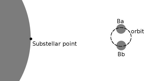
Figure 8: Sketch (not to scale) of the HD 181068 system.

In the following, we show that the variable force exerted on the surface of the giant HD 181068 A is similar to that exerted by a hot Jupiter on the surface of its host star. Because stellar rotation and orbital motion are typically not synchronized in planetary systems, the planet moves with respect to the stellar surface. This produces a variable but nonetheless periodic configuration of the planetary body and individual stellar surface elements and, thus, a periodic surface force potentially similar to that seen in HD 181068. A particularly intriguing example is a polar orbit during which the planet passes the stellar poles periodically, independent of the stellar rotation period (e.g., von Essen et al., 2014). This change in gravitational pull on the stellar atmosphere is among the proposed mechanisms for star-planet interaction (SPI), whose reality, however, remains controversial (e.g., Shkolnik et al., 2008; Scharf, 2010; Poppenhaeger et al., 2010).

In the HD 189733 system – a typical planetary system with a hot Jupiter – the gravitational acceleration caused by the planet HD 189733 b on the stellar atmosphere at the substellar point amounts to about $1$ cm s^-2 (see, e.g., Bouchy et al., 2005, for the orbital elements). Hence, the amplitude in local acceleration on the stellar surface caused by HD 189733 b is about a factor of $30$ larger than the amplitude of the periodic force at the substellar point in HD 181068. The latter is, however, sufficient to drive tidally-induced oscillations (Fuller et al., 2013); extrapolating, a similar interaction may be conceivable in HD 189733 and other comparable planetary systems. In contrast to HD 189733, however, HD 181068 A is a giant with a highly tenuous atmosphere and a surface gravity of only $\log(g)=2.73$, i.e., about two orders of magnitude below that of HD 189733 with $\log(g)=4.53\pm 0.14$ (Bouchy et al., 2005). Yet, in relation to the local gravity, the variable component is comparable in HD 181068 and HD 189733.

We conclude that hot Jovian planets revolving around main-sequence stars could cause observable changes in the stellar atmosphere analogous to the tidally driven oscillations observed in HD 181068. Whether this, however, produces any change, e.g., in the level or behavior of stellar activity remains unclear. At least in the case of HD 181068, we did not find any such relation: neither an elevated level of X-ray emission was found compared to other RS CVn systems nor a correlation between the flare timing and the orbital motion of the dwarf-binary could be identified.

6 Summary and conclusion

We have studied stellar activity in the hierarchical triple system HD 181068, using X-ray observations, Kepler light-curves, and an optical spectrum. With an S-index of $0.41\pm 0.01$ and a resulting $\log(R_{HK})$ value of $-4.52\pm 0.01$, HD 181068 A qualifies as an active – albeit not extremely active – giant member of an RS CVn system. This finding is compatible with the detection of quiescent X-ray emission at a level of $\approx 2\times 10^{31}$ erg s^-1 originating predominantly in the giant’s corona with a temperature distribution appropriately represented with a two-component thermal model peaked around $0.8$ keV and $1.9$ keV, and the presence of an inverse FIP effect. A comparison with the ROSAT survey, carried out more than a decade prior to our XMM-Newton program, did not reveal strong variability in the quiescent X-ray emission of HD 181068.

During the XMM-Newton observation on May 19, HD 181068 showed a three-fold elevated level of X-ray emission compared to the quiescent state with a clearly declining gradient and spectral hardness, which may have arisen from having observed the system during the decay phase of a flare. This is compatible with strong white-light flares observed in the Kepler light-curves, which likely originate on or close to the surface of the giant. The observed white-light flares release up to $6\times 10^{38}$ erg of energy in the Kepler band and potentially contribute significantly to the coronal heating. Although the observation on May 19 had been scheduled during secondary eclipse, the observed intrinsic variability prevented us from disentangling the contributions of the giant and the dwarf-binary. Based on coronal saturation, we estimated that at least $85$% of the observed X-ray emission must be attributed to the giant. Our findings are compatible with the hypothesis that strong magnetic activity suppresses solar-like oscillations in the giant.

As a result of its (internal) orbital motion, the dwarf-binary companion imposes a cyclic tidal distortion on the giant’s atmosphere, which shows up as an oscillation in the Kepler light-curve. Our estimates show that the cyclic gravitational force imposed on the substellar point of the giant’s surface is smaller in amplitude than the change in local surface gravity caused by a typical revolving hot Jupiter. Therefore, HD 181068 may serve as a model system to study star-planet-interactions. Based on the current sample of seven flares, we could not detect any correlation between the flare properties and the orbital motion of the AB- or dwarf-binary system. Further, the binary nature of HD 181068 B does not seem to have an impact on the giant’s bulk X-ray emission or activity if compared to other RS CVn systems; in fact, the X-ray properties of HD 181068 appear to be rather typical when compared to other RS CVn systems – a designation also adequate for HD 181068.