Charged Black Holes in a Five-dimensional Kaluza-Klein Universe

Abstract

We examine an exact solution which represents a charged black hole in a Kaluza-Klein universe in the five-dimensional Einstein-Maxwell theory. The spacetime approaches to the five-dimensional Kasner solution that describes expanding three dimensions and shrinking an extra dimension in the far region. The metric is continuous but not smooth at the black hole horizon. There appears a mild curvature singularity that a free-fall observer can traverse the horizon. The horizon is a squashed three-sphere with a constant size, and the metric is approximately static near the horizon.

I Introduction

Higher-dimensional spacetimes are investigated extensively in the context of unified theories. Spacetimes of the Kaluza-Klein type, non-compact three-dimensional space with compact extra dimensions of small size, would accord with effective four-dimensional spacetime. Black holes with compact extra dimensions, so-called Kaluza-Klein black holes, could be suitable for the model describing black holes that reside in our four-dimensional world. For example, five-dimensional squashed Kaluza-Klein black hole solutions Dobiasch:1981vh ; Gibbons:1985ac ; Gauntlett:2002nw ; Gaiotto:2005gf ; Ishihara:2005dp ; Wang:2006nw ; Yazadjiev:2006iv ; Nakagawa:2008rm ; Tomizawa:2008hw ; Tomizawa:2008rh ; Stelea:2008tt ; Tomizawa:2008qr ; Gal'tsov:2008sh ; Matsuno:2008fn ; Bena:2009ev ; Tomizawa:2010xq ; Mizoguchi:2011zj ; Chen:2010ih ; Stelea:2011fj ; Nedkova:2011hx ; Nedkova:2011aa ; Tatsuoka:2011tx ; Mizoguchi:2012vg ; Matsuno:2012hf ; Matsuno:2012ge ; Tomizawa:2012nk ; Stelea:2012ph ; Nedkova:2012yn ; Wu:2013nea ; Brihaye:2013vsa behave as fully five-dimensional black holes near the horizon and asymptote to the four-dimensional Minkowski spacetime with a compact extra dimension. The squashed black holes are constructed on the Gross-Perry-Sorkin (GPS) monopole solution Gross:1983 ; Sorkin:1983ns , and they have smooth horizons.

One of the important questions for the Kaluza-Klein spacetime model is why the size of extra dimensions are too small to detect by experiments. An interesting explanation is that the three-dimensional space expands while the extra dimensions shrink enough in the history of the universe Chodos:1979vk ; Sahdev:1988fp ; Ishihara:1984wx ; Ishihara:1986if . In the five-dimensional case, the (4+1)-dimensional Kasner solution, three-dimensional space expands while an extra dimension shrinks with the time evolution, provides such a model universe. Gibbons, Lu and Pope generalized the GPS monopole solution to dynamical ones Gibbons:2005rt , which nicely behaves as the Kasner universe in a distant region.

As generalizations of the Kastor-Traschen solution that describes charged black holes in de Sitter universe Kastor:1992nn , there exist a lot of solutions on higher-dimensional black holes for the Einstein-Maxwell system Maki:1992tq ; Klemm:2000vn ; Ishihara:2006ig ; Ida:2007vi ; Matsuno:2007ts ; Gibbons:2007zu , and brane solutions Gibbons:2005rt ; Maeda:2009zi in expanding universe models. All of these solutions are constructed using harmonic functions on four-dimensional Ricci flat spaces, where the harmonic functions contain the time-coordinate as a parameter. Time evolution of these spacetimes are driven by a cosmological constant, and then, all spatial dimensions expand in the laps of time.

In this paper, we investigate black hole solutions on the dynamical GPS monopole solution derived by Gibbons, Lu and Pope Gibbons:2005rt . Since a time slice of the dynamical GPS monopole solution is a Ricci flat space which has the time-variable as a parameter, by using suitable harmonic functions on the space we can construct an exact time-dependent solution in the five-dimensional Einstein-Maxwell theory. The solution approaches to the dynamical GPS monopole solution in the far region, expanding three dimensions and shrinking a compact dimension, then it describes a charged black hole in a Kaluza-Klein universe. What happens to the black hole when the extra dimension shrinks so that its size becomes smaller than the size of the black hole? To answer this question, we study geometrical properties of the solution.

This paper is organized as follows. We present the explicit form of the solution in Sec.II. The curvature singularities are studied in Sec.III. We give a C⁰ extension of the metric, and show that the solution describes a black hole in Sec.IV. Geometrical properties of the event horizon are also discussed. We summarize our results in Sec.V.

II Exact solution

We consider exact charged dynamical solutions in the five-dimensional Einstein-Maxwell theory with the action

$$S=\frac{1}{16\pi}\int d^{5}x\sqrt{-g}\left(R-F_{\mu\nu}F^{\mu\nu}\right).$$ (1)

The metric and the Maxwell field of the solutions are written as

$$ds^{2} = -H^{-2}dt^{2}+H\left[V(dr^{2}+r^{2}d\Omega^{2}_{\rm S^{2}})+N^{2}V^{-1}(d\psi+\cos\theta d\phi)^{2}\right],$$ (2)

$$A_{\mu}dx^{\mu} = \pm\frac{\sqrt{3}}{2}H^{-1}dt,$$ (3)

where $d\Omega^{2}_{\rm S^{2}}=d\theta^{2}+\sin^{2}\theta d\phi^{2}$ is the metric of unit two-dimensional sphere, S², and the functions $H$ and $V$ are given by

$$H = 1+\frac{M}{r},$$ (4)

$$V = \frac{t}{N}+\frac{N}{r},$$ (5)

where $M$ and $N$ are positive constants. As will be shown later, the metric describes black holes in an expanding Kaluza-Klein universe. The coordinates run the ranges of $-\infty<t<\infty,~{}-M<r<\infty,~{}0\leq\theta\leq\pi,~{}0\leq\phi\leq 2\pi$, and $0\leq\psi\leq 4\pi$. The angular part of the space consists twisted S¹ bundle over S².

If the parameter $M$ vanishes, the solution (2) coincides with the vacuum dynamical GPS monopole solution Gibbons:2005rt

$$ds^{2} = -dt^{2}+\left(\frac{t}{N}+\frac{N}{r}\right)(dr^{2}+r^{2}d\Omega^{2}_{\rm S^{2}})+N^{2}\left(\frac{t}{N}+\frac{N}{r}\right)^{-1}(d\psi+\cos\theta d\phi)^{2}.$$ (6)

It is easily seen by a coordinate transformation that the point $r=0$ on a time slice $t={\rm const.}$ is regular, and there is an initial singularity at $tr=-N^{2}$. In the limit $r\to+\infty$ with $t={\rm finite}$, the metric (2) as same as the metric (6) approaches to the five-dimensional Kasner-like metric with twisted S¹ in the form

$$ds^{2}\simeq-dt^{2}+\frac{t}{N}(dr^{2}+r^{2}d\Omega^{2}_{\rm S^{2}})+N^{2}\frac{N}{t}(d\psi+\cos\theta d\phi)^{2},$$ (7)

where the size of three-dimensional space increases and the size of S¹ decreases as the time $t$ laps Bizon:2006ue . It is clear that the metric (2) has a null infinity at $r=+\infty,~{}t=+\infty$ in the Kasner-like region. On the other hand, in the limit $r\to 0$ with $t={\rm finite}$, the metric (2) approaches

$$ds^{2}\simeq-\frac{r^{2}}{M^{2}}dt^{2}+\frac{MN}{r^{2}}dr^{2}+MN\left[d\Omega^{2}_{\rm S^{2}}+(d\psi+\cos\theta d\phi)^{2}\right].$$ (8)

It will be clarified, the metric (8) in the form of AdS${}_{2}\times$S³ does not describe near horizon geometry.

The black hole solution (2) is constructed on the dynamical GPS solution. If we take a Kaluza-Klein reduction of the metric (2) with respect to the Killing vector field $\partial/\partial\psi$, the obtained four-dimensional Einstein-Maxwell-dilaton solution coincides with that in Maeda:2009ds ; Maeda:2010ja .

III Curvature singularities

To examine the global structure of the spacetime with the metric (2), we first seek the locations of curvature singularities. The Kretschmann invariant and the square of the Maxwell field are

$$R^{\mu\nu\rho\sigma}R_{\mu\nu\rho\sigma} \propto \frac{1}{(M+r)^{6}(N^{2}+rt)^{6}},$$ (9)

$$F^{\mu\nu}F_{\mu\nu} \propto \frac{1}{(M+r)^{3}(N^{2}+rt)}.$$ (10)

We see that there are curvature singularities at $r=-M$ and $rt=-N^{2}$. These two singularities intersect at $t=N^{2}/M>0,~{}r=-M<0$ (see Fig.1).

For the spacetime signature $(-,+,+,+,+)$, the inequality $H(r)V(t,r)>0$ should be hold. Namely, we can consider three regions: (I) $r>0$, $rt>-N^{2}$, (II) $-M<r<0$, $rt>-N^{2}$, and (III) $r<-M$, $rt<-N^{2}$. Since the metric (2) in the region III describes a spacetime with a naked singularity, then we concentrate on the regions I and II. We will show, hereafter, that the metric (2) in the combined regions I and II represents a black hole.

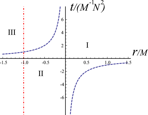
Figure 1: Curvature singularities are shown by dashed (blue) curves, $tr=-N^{2}$, and a dot-dashed (red) line, $r=-M$, in the $t$-$r$ plane. The metric (2) describes a spacetime with the signature $(-,+,+,+,+)$ in three regions: I ($r>0$, $rt>-N^{2}$), II ($-M<r<0$, $rt>-N^{2}$), and III ($r<-M$, $rt<-N^{2}$).

We consider the normal vector field $n^{(1)}_{\mu}dx^{\mu}=dr$ to the $r={\rm const.}$ surfaces. The norm of the vector field is given by

$$g^{\mu\nu}n^{(1)}_{\mu}n^{(1)}_{\nu}=H^{-1}V^{-1}.$$ (11)

Since the norm is positive in the region II, then the curvature singularity $r=-M$ in the region II is timelike.

We also consider the normal vector field $n^{(2)}_{\mu}dx^{\mu}=rdt+tdr$ to the $rt={\rm const.}$ surfaces. The norm of the vector is

$$g^{\mu\nu}n^{(2)}_{\mu}n^{(2)}_{\nu}=-H^{2}r^{2}+H^{-1}V^{-1}t^{2}$$ (12)

In the limit $rt\to-N^{2}$ in the regions I and II, the norm (12) becomes $+\infty$. Then, the curvature singularities $rt=-N^{2}$ in the both region I and II are timelike.

IV Extension of Spacetime

IV.1 New Coordinates

The metric (2) has an apparent singularity at $r=0$. We investigate the possibility of extension by using null geodesics starting from the region $r>0$.

If we restrict ourselves to the null geodesics confined in the $t$-$r$ plane, i.e., $\theta={\rm const.}$, $\phi={\rm const.}$, $\psi={\rm const.}$, the null geodesics are determined by the null condition,

$$-H^{-2}dt^{2}+HVdr^{2}=0.$$ (13)

Then, we have

$$\left(\frac{dt}{dr}\right)^{2}=\frac{(r+M)^{3}(tr+N^{2})}{Nr^{4}}.$$ (14)

For ingoing future null geodesics, increasing $t$ and decreasing $r$, we see that $t$ should diverge as $r\to 0$ with $tr=\text{finite}$. The null geodesics terminate the coordinate boundary $r\to 0$ with $tr=\text{finite}$. Then, we try to extend the metric there.

In many cases, a set of null geodesics is a powerful tool to construct coordinates covering the black hole horizons. Unfortunately, in our case, we hardly solve (14) in analytic form. Then, we use curves that are approximate solutions for (14) in the vicinity of $r=0$. We assume the approximate solutions in the form,

$$tr=a+ur^{b}+cr,$$ (15)

where $a,~{}b,~{}c$ are constants, and $u$ is an arbitrary parameter. Substituting (15) into (14), and taking the limit $r\to 0$, we can determine the constants $a,~{}b,~{}c$ as

$$a = \frac{M^{3}}{2N}\left(1+\sqrt{1+\frac{4N^{3}}{M^{3}}}\right),$$ (16)

$$b = 1-\frac{M^{3}}{2aN}=1-\frac{1}{1+\sqrt{1+4N^{3}/M^{3}}},$$ (17)

$$c = -\frac{3(a+N^{2})}{M}=-\frac{3M^{2}}{2N}\left(1+\frac{2N^{3}}{M^{3}}+\sqrt{1+\frac{4N^{3}}{M^{3}}}\right).$$ (18)

The constant $b$ takes a value in the range $1/2<b<1$.

The curves (15) with (16)-(18) are approximately ingoing future null geodesics that attain the coordinate boundary. The free parameter $u$, which labels the curves, can be used as a new coordinate.

Now, we introduce new coordinates $(\rho,~{}u)$ as

$$\rho=r^{b},\quad u=\frac{(t-c)r-a}{r^{b}},$$ (19)

then the metric (2) and the Maxwell field (3) take the forms,

$$ds^{2} = -\frac{\rho^{2}}{H^{\prime 2}}du^{2}+2\frac{L}{bH^{\prime 2}}dud\rho+\frac{H^{\prime 3}K-NL^{2}}{b^{2}NH^{\prime 2}\rho^{2}}d\rho^{2}$$ (20)

$$\qquad+\frac{H^{\prime}K}{N}d\Omega_{\rm S^{2}}^{2}+\frac{H^{\prime}N^{3}}{K}(d\psi+\cos\theta d\phi)^{2},$$

$$A_{\mu}dx^{\mu} = \pm\frac{\sqrt{3}}{2H^{\prime}}\left[\rho du-\frac{L}{b\rho}d\rho\right],$$ (21)

where

$$H^{\prime}=M+\rho^{1/b},\quad K=N^{2}+a+u\rho+c\rho^{1/b},\quad L=a+(1-b)u\rho.$$ (22)

In the limit $\rho\to 0$ with $u={\rm finite}$, (equivalently, $r\to 0$ with $tr=a$ ), the metric (20) and the Maxwell field (21) behave as

$$ds^{2} \to \frac{2a}{bM^{2}}dud\rho-\frac{M^{4}}{4a^{2}b^{2}N^{2}}u^{2}d\rho^{2}+M\frac{N^{2}+a}{N}d\Omega_{\rm S^{2}}^{2}+\frac{MN^{3}}{N^{2}+a}(d\psi+\cos\theta d\phi)^{2},$$ (23)

$$A_{\mu}dx^{\mu} \to \pm\frac{\sqrt{3}M^{2}}{4abN}ud\rho,$$ (24)

where a pure gauge term $\rho^{-1}d\rho$ in $A_{\mu}dx^{\mu}$ is omitted. The metric, which represents AdS${}^{2}\times$(squashed S³), and the Maxwell field are regular at $\rho=0$. We also see that the $\rho=0$ surface is a null surface, and the angular part of the metric, which describes a squashed S³, does not depend on the time at $\rho=0$. It means that expansion of outgoing null bundle emanating from the squashed S³ on a time slice $u={\rm const.}$ is vanishing at $\rho=0$. The area of the squashed S³ at $\rho=0$ is given by

$$A_{\text{H}}=\sqrt{M^{3}N(N^{2}+a)}A_{\rm S^{3}},$$ (25)

where $A_{\rm S^{3}}$ denotes the area of a unit S³.

IV.2 Extension

Here, we extend the metric across the $\rho=0$ surface. Similar to the discussion in Tatsuoka:2011tx , we assume that the function $L$ in (22) is used globally, and the functions $H^{\prime}$ and $K$ in (22), which contain $\rho^{1/b}$, are extended as

$$H^{\prime}=M+\Theta(\rho)~{}|\rho|^{1/b},\quad K=N^{2}+a+u\rho+c~{}\Theta(\rho)~{}|\rho|^{1/b},\quad L=a+(1-b)u\rho,$$ (26)

where $\Theta(\rho)$ denotes a step function, $\Theta(\rho)=+1~{}(\rho\geq 0),~{}-1~{}(\rho<0)$. The metric (20) and the Maxwell field (21) with (26) are continuous at $\rho=0$.

Introducing new coordinates $r^{\prime}(<0)$ and $t^{\prime}$ in the $\rho<0$ region by

$$\rho=-(-{r^{\prime}})^{b},\quad u=\frac{(t^{\prime}-c)(-r^{\prime})+a}{(-{r^{\prime}})^{b}},$$ (27)

we show that the metric (20) and the Maxwell field (21) with (26) reproduce

$$ds^{2} = -\left(1+\frac{M}{r^{\prime}}\right)^{-2}dt^{\prime 2}+\left(1+\frac{M}{r^{\prime}}\right)\left[\left(\frac{t^{\prime}}{N}+\frac{N}{r^{\prime}}\right)(d{r^{\prime}}^{2}+{r^{\prime}}^{2}d\Omega^{2}_{\rm S^{2}})\right.$$ (28)

$$\qquad\qquad\left.+N^{2}\left(\frac{t^{\prime}}{N}+\frac{N}{r^{\prime}}\right)^{-1}(d\psi+\cos\theta d\phi)^{2}\right],$$

$$A_{\mu}dx^{\mu} = \pm\frac{\sqrt{3}}{2}\left(1+\frac{M}{r^{\prime}}\right)^{-1}dt^{\prime}.$$ (29)

The metric and the Maxwell field coincide with the metric (2) and the Maxwell field (3) with $r^{\prime}<0$. Then it is clear that the spacetime with the metric (20) with (26) gives a C⁰ extension of the metric (2) in the region I to the region II. That is, the null boundary $r\to 0_{+},t\to\infty$ with $rt=a$ in the region I is attached the null boundary $r\to 0_{-},t\to-\infty$ with $rt=a$ in the region II.

The outer region I becomes asymptotically the Kasner-like universe described by (7), then it has a null infinity. However, any null geodesic starting from a point in the inner region II cannot reach the null infinity. Therefore, the $\rho=0$ surface is an event horizon. The exact solution (2) with (3) indeed represents the charged black hole in the five-dimensional anisotropically expanding Kaluza-Klein universe. We see by the metric (23) that the horizon shape is not a round S³ but the squashed S³. The area of the event horizon is independent of the time.

IV.3 Penrose diagram

According to the extension in the previous subsection, the Penrose diagram of the solution (2) is shown in the Fig.2.

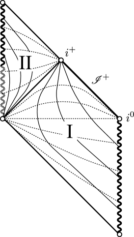
Figure 2: Penrose diagram of $t-r$ plane. The outer region I and the inner region II are joined at the event horizon, $r=0$ and $rt=a$. The null infinity exists at $r=+\infty$ and $t=+\infty$. The wavy lines are curvature singularities. Dashed curves denote $t={\rm const.}$ surfaces, and thin solid curves denote $r={\rm const.}$ surfaces.

In the outer region I, the geometry looks like the anisotropic Kasner universe described by (7) in the far region, $r\gg N,M$, where the three-dimensional space expands infinitely, while the compact extra dimension shrinks with the time evolution. There is a null infinity at $r=+\infty,~{}t=+\infty$. There also exists a timelike singularity at $rt=-N^{2}$. In the inner region II, there are timelike singularities at $r=-M<0$ and $rt=-N^{2}$. Two regions I and II are attached at the event horizon $\rho=0$ in the new coordinate, that is, at the coordinate boundary in the old coordinates $r=0_{\pm},~{}t=\pm\infty$ with $tr=a={\rm finite}$.

We have the metric with all of the components are continuous at the event horizon. Although the metric is not smooth at the horizon, the Kretschmann invariant is finite there, and components of the Ricci tensor are finite in regular coordinate basis, $du$ and $d\rho$. We find, however, that some components of Riemann curvature diverge there.

The singularity on the horizon is relatively mild. For example, a component of Riemann curvature diverges at $\rho=0$ as

$$R_{\theta\rho\theta\rho}\propto\rho^{-2+1/b},$$ (30)

where $1/b$ takes a value in the range $1<1/b<2$. Because the integration of the curvature component in an infinitesimal segment across the horizon:

$$\int_{-\epsilon}^{+\epsilon}d\rho R_{\theta\rho\theta\rho}$$ (31)

is finite, the tidal force causes finite difference in deviation of geodesic congruence crossing the horizon. Then, the singularity is relatively mild so that an observer can traverse the horizon.

We have extended the metric across the surface $r=0$ and $t=\infty$ to clarify the spacetime is black hole. Although the coordinate boundaries $r=0_{+}$ and $t=-\infty$ in the region I, and $r=0_{-}$ and $t=+\infty$ in the region II would be extendible, explicit extension is not done yet.

IV.4 Static geometry near event horizon

The spacetime is dynamical because the metric (2) does not admit any timelike Killing vector. However, (23) means the size of event horizon, given by (25), is constant during evolution of the universe.

To observe the geometry near horizon clearly, we consider the limit $r\to 0_{+},~{}t\to\infty$ keeping $rt\to{\rm finite}$ of the metric (2). In this limit the metric has the form of

$$ds^{2}\simeq-\frac{r^{2}}{M^{2}}dt^{2}+\frac{M(rt+N^{2})}{Nr^{2}}dr^{2}+\frac{M(rt+N^{2})}{N}d\Omega^{2}_{\rm S^{2}}+\frac{MN^{3}}{rt+N^{2}}(d\psi+\cos{\theta}d\phi)^{2}.$$ (32)

Introducing coordinates

$$\tilde{\rho}^{2}=\frac{M}{N}(rt+N^{2}),\quad\tau=\frac{N}{M^{2}}\log t,$$ (33)

we see the metric (32) becomes

$$ds^{2} \simeq -f(\tilde{\rho})d\tau^{2}-\frac{4M^{2}\tilde{\rho}^{3}}{N(\tilde{\rho}^{2}-MN)}d\tau d\tilde{\rho}+\frac{4\tilde{\rho}^{4}}{(\tilde{\rho}^{2}-MN)^{2}}d\tilde{\rho}^{2}$$ (34)

$$\qquad+\tilde{\rho}^{2}d\Omega^{2}_{\rm S^{2}}+\frac{M^{2}N^{2}}{\tilde{\rho}^{2}}(d\psi+\cos{\theta}d\phi)^{2},$$

$$f(\tilde{\rho}) = (\tilde{\rho}^{2}-\tilde{\rho}^{2}_{+})(\tilde{\rho}^{2}-\tilde{\rho}^{2}_{-}),\quad\tilde{\rho}_{\pm}^{2}=\frac{M(M^{3}+2N^{3})\pm\sqrt{M^{5}(M^{3}+4N^{3})}}{2N^{2}}.$$ (35)

Further, introducing a coordinate

$$dT=d\tau+\frac{2M^{2}\tilde{\rho}^{3}}{N(\tilde{\rho}^{2}-MN)f(\tilde{\rho})}d\tilde{\rho},$$ (36)

we have the metric (34) in the form

$$ds^{2}\simeq-f(\tilde{\rho})dT^{2}+\frac{4\tilde{\rho}^{4}}{f(\tilde{\rho})}d\tilde{\rho}^{2}+\tilde{\rho}^{2}d\Omega^{2}_{\rm S^{2}}+\frac{M^{2}N^{2}}{\tilde{\rho}^{2}}(d\psi+\cos{\theta}d\phi)^{2}.$$ (37)

This metric is a limiting case of static charged squashed Kaluza-Klein black hole solutions derived in ref. Ishihara:2005dp . Taking the limit that the asymptotic size of the extra dimension becomes zero, the charged squashed Kaluza-Klein metric reduces to (37). It is clear that the event horizon is static.

At the late stage, the three-dimensional distances between observers at $r={\rm const.}\neq 0$ and constant angular coordinates increase by the cosmological scale factor $\sim\sqrt{t}$, and the size of the extra dimension shrinks as $\sim 1/\sqrt{t}$. Nevertheless, near black hole region, i.e., $r\to 0,~{}t\to\infty$ with $rt={\rm const.}$, for an observer at a finite circumference distance $\tilde{\rho}$ the size of extra dimension is the finite time-independent value $MN/\tilde{\rho}$.

It is also clear from (37) that the horizon is non-degenerate though the metric is constructed by using the harmonic function $H$ on a Ricci flat base space, in contrast to stationary extremal charged black holes, which have degenerate horizons. This is similar to the cosmological charged black holes with a cosmological constant Ida:2007vi .

IV.5 Expansion of a null congruence

Here we calculate the expansions of the null vector fields emanating from the closed surface $r={\rm const.}$ on a $t={\rm const.}$ slice. The expansions are defined by

$$\theta^{\pm}=h^{\mu\nu}\nabla_{\mu}k^{(\pm)}_{\nu},$$ (38)

where $k^{(+)\mu}\partial_{\mu}$ and $k^{(-)\mu}\partial_{\mu}$ denote future null vector fields. We choose the null vector fields $k^{(\pm)\mu}\partial_{\mu}$ such that

$$k^{(+)\mu}\frac{\partial}{\partial x^{\mu}} = \frac{1}{\sqrt{2}}\frac{\partial}{\partial t}+\frac{1}{H\sqrt{2HV}}\frac{\partial}{\partial r},$$ (39)

$$k^{(-)\mu}\frac{\partial}{\partial x^{\mu}} = \frac{H^{2}}{\sqrt{2}}\frac{\partial}{\partial t}-\sqrt{\frac{H}{2V}}\frac{\partial}{\partial r},$$ (40)

where $k^{(\pm)}$ are null vectors in the direction of increasing/decreasing $r$ coordinate, respectively. The vectors $k^{(\pm)}$ are regular in the far region, $r\gg M,N$, and they satisfy the relations $k^{(-)\mu}\nabla_{\mu}k^{(-)\nu}=0$ , and $g_{\mu\nu}k^{(+)\mu}k^{(-)\nu}=-1$. Then, they are regular everywhere. The metric on S³ ($r={\rm const.}$, $t={\rm const.}$), $h_{\mu\nu}$, is given by

$$h_{\mu\nu}=g_{\mu\nu}+k^{(+)}_{\mu}k^{(-)}_{\nu}+k^{(+)}_{\nu}k^{(-)}_{\mu}.$$ (41)

In the case of (39) and (40), $h_{\mu\nu}$ becomes

$$h_{\mu\nu}dx^{\mu}dx^{\nu}=HVr^{2}d\Omega^{2}_{\rm S^{2}}+N^{2}HV^{-1}(d\psi+\cos\theta d\phi)^{2}.$$ (42)

The expansions of null geodesic congruences on the three-dimensional space (42) are obtained as

$$\theta^{+} = \frac{rH^{2}\sqrt{HV}+\left(3NV+tH\right)}{2\sqrt{2}NrH^{5/2}V^{3/2}},$$ (43)

$$\theta^{-} = \frac{rH^{2}\sqrt{HV}-\left(3NV+tH\right)}{2\sqrt{2}NrH^{1/2}V^{3/2}}.$$ (44)

In the limit $r\to 0,~{}t\to\infty$ with $tr=a$, $\theta^{+}=0$ and $\theta^{-}={\rm const.}<0$. Then we see that the event horizon, $r=0,~{}t=\infty$ with $tr=a$ surface, is an apparent horizon.

We show the sign of $\theta^{\pm}$ in the Penrose diagrams in the Fig.3. We can see that outside the black hole, $r>0$, there is a region of $(\theta^{+},\theta^{-})=(+,+)$ like an expanding universe, while inside the black hole, $r<0$, there is a trapped region $(\theta^{+},\theta^{-})=(-,-)$ .

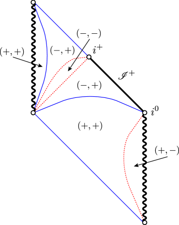
Figure 3: The sign of $\theta^{\pm}$ in the Penrose diagram. Pairs of $(\pm,\pm)$ denote the sign of $(\theta^{-},\theta^{+})$. Dotted (red) curves and solid (blue) curves denote $\theta^{+}=0$ and $\theta^{-}=0$ surfaces, respectively.

V Summary

We examine the exact solution which represents a charged black hole resides in a five-dimensional Kasner-like universe in the Einstein-Maxwell theory. Outside of the black hole horizon, $r>0$, the metric approaches to the five-dimensional Kasner-like universe, where three-dimensional space expands while a compact extra dimension shrinks, in the far region. The universe has a future null infinity in the late time and a timelike singularity in the early stage. Inside of the black hole horizon, $r<0$, there are also timelike singularities. We give a C⁰ extension of the spacetime across the event horizon $r=0$. Thus the solution represents the charged black hole sitting in the dynamical Kaluza-Klein universe. The shape of the horizon is a squashed S³, and its area does not depend on the time though the spacetime is dynamical.

The metric is not smooth at the horizon. Even though the Kretschmann invariant is finite, some components of Riemann curvature in a regular basis diverge at the horizon. The curvature singularity is relatively mild because an integration of the curvature in an infinitesimal segment across the horizon is finite. Therefore, a free-falling observer can traverse the horizon. In contrast to the fact that the five-dimensional stationary squashed Kaluza-Klein black hole solutions Dobiasch:1981vh ; Gibbons:1985ac ; Gauntlett:2002nw ; Gaiotto:2005gf ; Ishihara:2005dp ; Wang:2006nw ; Yazadjiev:2006iv ; Nakagawa:2008rm ; Tomizawa:2008hw ; Tomizawa:2008rh ; Stelea:2008tt ; Tomizawa:2008qr ; Gal'tsov:2008sh ; Matsuno:2008fn ; Bena:2009ev ; Tomizawa:2010xq ; Mizoguchi:2011zj ; Chen:2010ih ; Stelea:2011fj ; Nedkova:2011hx ; Tatsuoka:2011tx ; Nedkova:2011aa ; Mizoguchi:2012vg ; Matsuno:2012hf ; Matsuno:2012ge ; Tomizawa:2012nk ; Stelea:2012ph ; Nedkova:2012yn ; Wu:2013nea ; Brihaye:2013vsa have smooth horizons, the five-dimensional dynamical Kaluza-Klein black hole has weakly singular event horizon. This is similar to the extremal charged Kaluza-Klein black hole solutions Tatsuoka:2011tx in the case of higher than five dimensions.

Numbers of extremal charged stationary black hole solutions are constructed by using harmonic functions on Ricci flat base spaces. In these cases, black hole horizons are degenerate. Similarly, the solution in the present paper is constructed by a harmonic function on a Ricci flat base space. However, the base space in the present case has the time-variable as a parameter. This is the reason why the solution is dynamical. Resultant black hole has non-degenerate horizon in this case. It is worth noting that the set of metric and Maxwell field is also a solution of the Einstein-Maxwell-Chern-Simons system.

In the late time, though the size of extra dimension in the far region shrinks to a smaller size than that of the black hole, the event horizon does not change in its size. Indeed, the total spacetime is dynamical, but the geometry of near the event horizon is static. The expansion of the outgoing null geodesic congruence emanating from the event horizon is vanishing, i.e., the event horizon is an apparent horizon even though the spacetime is dynamical. We can understand this result as follows. In static vacuum Kaluza-Klein black hole solutions Dobiasch:1981vh ; Gibbons:1985ac , the horizons are flattened as the size parameters of the extra dimension become small. In contrast, in the case of charged Kaluza-Klein black holes Ishihara:2005dp , the horizon can be fat and round against to the small extra dimension. Thus, we would expect that the existence of electric charge stabilizes the size of black hole against shrinking extra dimension of the Kaluza-Klein universe in the present solution.

The solution (2) can be easily generalized to multi-black hole solution. In this solution, the metric (2), the harmonic functions (4) and (5) are replaced by

$$ds^{2} = -H^{-2}dt^{2}+H\left[V(dx^{2}+dy^{2}+dz^{2})+V^{-1}(d\zeta+\bm{\omega})^{2}\right],$$ (45)

$$H = 1+\sum_{i}\frac{M_{i}}{|\bm{x}-\bm{x}_{i}|},$$ (46)

$$V = \frac{t}{t_{0}}+\sum_{i}\frac{N_{i}}{|\bm{x}-\bm{x}_{i}|},$$ (47)

where the 1-form $\bm{\omega}$ is determined by $\nabla\times\bm{\omega}=\nabla V$, and $t_{0},~{}M_{i},~{}N_{i}$ are positive constants, and $\bm{x}=(x,~{}y,~{}z),~{}\bm{x}_{i}=(x_{i},~{}y_{i},~{}z_{i})$ denotes position vectors on the three-dimensional Euclid space. The metric (45) with the harmonic functions (46) and (47) would describe the multi-black holes. We leave the analysis for the future.

References

- (1) P. Dobiasch and D. Maison, Gen. Rel. Grav. 14, 231 (1982).
- (2) G. W. Gibbons and D. L. Wiltshire, Annals Phys. 167, 201 (1986) [Erratum-ibid. 176, 393 (1987)].
- (3) J. P. Gauntlett, J. B. Gutowski, C. M. Hull, S. Pakis and H. S. Reall, Class. Quant. Grav. 20, 4587 (2003) [arXiv:hep-th/0209114].
- (4) D. Gaiotto, A. Strominger, X. Yin, JHEP 0602, 024 (2006). [hep-th/0503217].
- (5) H. Ishihara and K. Matsuno, Prog. Theor. Phys. 116, 417 (2006) [arXiv:hep-th/0510094].
- (6) T. Wang, Nucl. Phys. B 756, 86 (2006) [hep-th/0605048].
- (7) S. S. Yazadjiev, Phys. Rev. D74, 024022 (2006). [hep-th/0605271].
- (8) T. Nakagawa, H. Ishihara, K. Matsuno and S. Tomizawa, Phys. Rev. D 77, 044040 (2008) [arXiv:0801.0164 [hep-th]].
- (9) S. Tomizawa, H. Ishihara, K. Matsuno and T. Nakagawa, Prog. Theor. Phys. 121, 823 (2009) [arXiv:0803.3873 [hep-th]].
- (10) K. Matsuno, H. Ishihara, T. Nakagawa and S. Tomizawa, Phys. Rev. D 78, 064016 (2008) [arXiv:0806.3316 [hep-th]].
- (11) S. Tomizawa and A. Ishibashi, Class. Quant. Grav. 25, 245007 (2008) [arXiv:0807.1564 [hep-th]].
- (12) C. Stelea, K. Schleich and D. Witt, Phys. Rev. D 78, 124006 (2008) [arXiv:0807.4338 [hep-th]].
- (13) S. Tomizawa, Y. Yasui, Y. Morisawa, Class. Quant. Grav. 26, 145006 (2009). [arXiv:0809.2001 [hep-th]].
- (14) D. V. Gal’tsov and N. G. Scherbluk, Phys. Rev. D 79, 064020 (2009) [arXiv:0812.2336 [hep-th]].
- (15) I. Bena, G. Dall’Agata, S. Giusto, C. Ruef, N. P. Warner, JHEP 0906, 015 (2009). [arXiv:0902.4526 [hep-th]].
- (16) S. Tomizawa, arXiv:1009.3568 [hep-th].
- (17) S. ’y. Mizoguchi, S. Tomizawa, Phys. Rev. D84, 104009 (2011). [arXiv:1106.3165 [hep-th]].
- (18) Y. Chen and E. Teo, Nucl. Phys. B 850, 253 (2011) [arXiv:1011.6464 [hep-th]].
- (19) C. Stelea, K. Schleich and D. Witt, arXiv:1108.5145 [gr-qc].
- (20) P. G. Nedkova and S. S. Yazadjiev, Phys. Rev. D 84, 124040 (2011) [arXiv:1109.2838 [hep-th]].
- (21) T. Tatsuoka, H. Ishihara, M. Kimura and K. Matsuno, Phys. Rev. D 85, 044006 (2012) [arXiv:1110.6731 [hep-th]].
- (22) P. G. Nedkova and S. S. Yazadjiev, Phys. Rev. D 85, 064021 (2012) [arXiv:1112.3326 [hep-th]].
- (23) S. ’y. Mizoguchi and S. Tomizawa, Phys. Rev. D 86, 024022 (2012) [arXiv:1201.3063 [hep-th]].
- (24) K. Matsuno, H. Ishihara, M. Kimura and T. Tatsuoka, Phys. Rev. D 86, 044036 (2012) [arXiv:1206.4818 [hep-th]].
- (25) K. Matsuno, H. Ishihara, M. Kimura and T. Tatsuoka, Phys. Rev. D 86, 104054 (2012) [arXiv:1208.5536 [hep-th]].
- (26) S. Tomizawa and S. ’y. Mizoguchi, Phys. Rev. D 87, 024027 (2013) [arXiv:1210.6723 [hep-th]].
- (27) C. Stelea, C. Dariescu and M. A. Dariescu, Phys. Rev. D 87, 024039 (2013) [arXiv:1211.3154 [gr-qc]].
- (28) P. G. Nedkova and S. S. Yazadjiev, Eur. Phys. J. C 73, 2377 (2013) [arXiv:1211.5249 [hep-th]].
- (29) S. -Q. Wu, D. Wen, Q. -Q. Jiang and S. -Z. Yang, Phys. Lett. B 726, 404 (2013) [arXiv:1311.7222 [hep-th]].
- (30) Y. Brihaye and E. Radu, JHEP 1311, 049 (2013) [arXiv:1305.3531 [gr-qc]].
- (31) D. J. Gross and M. J. Perry, Nucl. Phys. B 226, 29 (1983).
- (32) R. d. Sorkin, Phys. Rev. Lett. 51, 87 (1983).
- (33) A. Chodos and S. L. Detweiler, Phys. Rev. D 21, 2167 (1980).
- (34) D. Sahdev, Phys. Lett. B 137, 155 (1984).
- (35) H. Ishihara, Prog. Theor. Phys. 72, 376 (1984).
- (36) H. Ishihara, Phys. Lett. B 179, 217 (1986).
- (37) G. W. Gibbons, H. Lu and C. N. Pope, Phys. Rev. Lett. 94, 131602 (2005) [hep-th/0501117].
- (38) D. Kastor and J. H. Traschen, Phys. Rev. D 47, 5370 (1993) [hep-th/9212035].
- (39) T. Maki and K. Shiraishi, Class. Quant. Grav. 10, 2171 (1993) [arXiv:1403.1320 [gr-qc]].
- (40) D. Klemm and W. A. Sabra, Phys. Lett. B 503, 147 (2001) [hep-th/0010200].
- (41) H. Ishihara, M. Kimura and S. Tomizawa, Class. Quant. Grav. 23, L89 (2006) [hep-th/0609165].
- (42) D. Ida, H. Ishihara, M. Kimura, K. Matsuno, Y. Morisawa and S. Tomizawa, Class. Quant. Grav. 24, 3141 (2007) [hep-th/0702148 [HEP-TH]].
- (43) K. Matsuno, H. Ishihara, M. Kimura and S. Tomizawa, Phys. Rev. D 76, 104037 (2007) [arXiv:0707.1757 [hep-th]].
- (44) G. W. Gibbons and C. N. Pope, Class. Quant. Grav. 25, 125015 (2008) [arXiv:0709.2440 [hep-th]].
- (45) K. -i. Maeda, N. Ohta and K. Uzawa, JHEP 0906, 051 (2009) [arXiv:0903.5483 [hep-th]].
- (46) K. -i. Maeda and M. Nozawa, Phys. Rev. D 81, 044017 (2010) [arXiv:0912.2811 [hep-th]].
- (47) K. -i. Maeda and M. Nozawa, Phys. Rev. D 81, 124038 (2010) [arXiv:1003.2849 [gr-qc]].
- (48) P. Bizon, T. Chmaj and G. Gibbons, Phys. Rev. Lett. 96, 231103 (2006) [gr-qc/0604043].