Motor proteins traffic regulation by supply-demand balance of resources

Abstract

In cells and in vitro assays the number of motor proteins involved in biological transport processes is far from being unlimited. The cytoskeletal binding sites are in contact with the same finite reservoir of motors (either the cytosol or the flow chamber) and hence compete for recruiting the available motors, potentially depleting the reservoir and affecting cytoskeletal transport. In this work we provide a theoretical framework to study, analytically and numerically, how motor density profiles and crowding along cytoskeletal filaments depend on the competition of motors for their binding sites. We propose two models in which finite processive motor proteins actively advance along cytoskeletal filaments and are continuously exchanged with the motor pool. We first look at homogeneous reservoirs and then examine the effects of free motor diffusion in the surrounding medium. We consider as a reference situation recent in vitro experimental setups of kinesin-8 motors binding and moving along microtubule filaments in a flow chamber. We investigate how the crowding of linear motor proteins moving on a filament can be regulated by the balance between supply (concentration of motor proteins in the flow chamber) and demand (total number of polymerised tubulin heterodimers). We present analytical results for the density profiles of bound motors, the reservoir depletion, and propose novel phase diagrams that present the formation of jams of motor proteins on the filament as a function of two tuneable experimental parameters: the motor protein concentration and the concentration of tubulins polymerized into cytoskeletal filaments. Extensive numerical simulations corroborate the analytical results for parameters in the experimental range and also address the effects of diffusion of motor proteins in the reservoir. We then propose experiments to validate our models and discuss how the ”supply-demand” effects can regulate motor traffic also in in vivo conditions.

Keywords: Molecular motors, Finite resources, Exclusion processes, Stochastic modeling

1 Introduction

Linear motor proteins are ATPase-driven machines that bind to cytoskeletal polar filaments and perform linear directed motion along them [1, 2, 3]. They are classified into three superfamilies, kinesins, dyneins and myosins [4]. These motor proteins regulate many intracellular processes that are necessary to create and maintain the high level of organization inside the cell, in particular active transport and force production. Active transport driven by motor proteins indeed is essential to carry cargoes (i.e. proteins, organelles, metabolites, etc.) over long enough distances when diffusion becomes ineffective, e.g. in eukaryotic cilia [5, 6] and axons [7, 8, 9]. Motor proteins control the transport of organelles in various intracellular processes such as endo- and exocytosis, and are therefore major actors in membrane traffic phenomena [1]. Viruses too can take advantage of directed transport by binding motor proteins to reach the cell core [10]. Moreover, motor proteins are involved into other processes not directly related to cargo transport [11], for example the length regulation of cytoskeletal filaments [12, 13]. Recent experimental studies [12, 13, 14] have focused on Kip3, the highly processive kinesin-8 motor of budding yeast moving along microtubule filaments. In these in vitro experiments Kip3 diffuses in a solution and binds to the microtubules attached to the slide of the flow chamber [12, 13, 14]. By means of fluorophore labeling the authors reconstructed the steady-state density profiles of motors on the microtubules, and found clear evidence of density shocks whereby a queue of motors accumulates from the end tip of the filament. These findings have been interpreted within the framework of a previously developed model: the totally asymmetric simple exclusion process with Langmuir kinetics (TASEP-LK_∞) [15, 16]. This model exhibits bulk-localized shocks of particles that have been called domain walls. These kind of density discontinuities are the result of exclusion interactions between particles, attachment/detachment dynamics of particles on the filament, and the presence of a flow bottleneck at the end tip. Such a model allows us to quantitatively characterize the motor density profiles on the filament in terms of microscopic parameters and determine the physical conditions under which traffic jams arise. The latter is also of interest to biological questions, for instance, in understanding whether the conditions in vivo are such that the formation of jams is avoided [14].

The in vitro experiments [13, 14] are performed at high motor protein concentrations and low concentrations of tubulin dimers. In this way, the reservoir of motors can be considered as unlimited and no depletion of motors diffusing in the chamber is observed. Therefore, the modelling approach introduced with the TASEP-LK_∞ [15, 16] is a good approximation of the system studied in [14], and it provides testable predictions of the corresponding experiments. However, at lower motor protein concentrations, or higher concentrations of tubulins, the attachment kinetics leads to depletion of motors that could severely affect the overall exchange of of motors between the filament and the reservoir.

Here we extend motor protein transport models studied in the literature (such as the TASEP-LK_∞) by considering the limited availability of resources in the reservoir. Using these models we thus develop a theoretical framework that allows us to address the reservoir depletion in in vitro experiments performed at motor protein concentrations that are low with respect to the concentrations of polymerized tubulin heterodimers. In this regime of limited resources the results of our modelling framework are expected to deviate qualitatively from TASEP-LK_∞.

We study the reservoir depletion effects on motor protein transport using two different models. The first model is a totally asymmetric simple exclusion process in contact with a finite homogeneous reservoir composed of a limited number of particles. As it will be justified later, we call this model TASEP-LK_m. The TASEP-LK_m adds the concentration of binding sites (i.e. the total concentration of tubulin dimers available for the binding kinesins) as a new control parameter to the TASEP-LK_∞ model. The second model that we analyze consists in an exclusion process in contact with a diffusive reservoir in which unbound particles freely diffuse at a finite rate (similar to the models defined, e.g., in [17, 18, 19, 20, 21, 22]). Note that the influence of a limited reservoir on the transport of molecular motors have already been studied for ribosomes [23, 24, 25]. There is however an important difference between the dynamics of motor proteins and ribosomes: while the former can detach and attach at any filament binding site, the latter only attach/detach at the first/last site of the filament, making the mathematical treatment less elaborate.

Our results allow us to study the competition between the filaments binding sites for the number of proteins in the reservoir, and investigate its impact on transport phenomena driven by motor proteins. We address analytically and numerically how this competition for finite resources influences the density profile of motor proteins and the formation of jams on the filament. In particular, we describe how the density profile depends on the ratio between the concentration of motor proteins and the cytoskeletal binding site concentrations. Our results could be tested in in vitro and in vivo experiments of molecular motors moving along biofilaments such as the ones presented in [14, 26, 27], by administering motor protein concentrations that are lower or comparable to the concentration of tubulin dimers.

In section 2 we define the models we use to describe motor protein transport at limited availability of resources. In section 3 we present the transport equations for TASEP-LK_m in the continuum limit of a mean field approximation. We analytically solve the equations and derive the expressions for the density profiles of bound motors, determine the parameter regimes for which we expect jam formation, and obtain the dependence of the jam length on the supply and demand of resources. In section 4 we present the outcomes of numerical simulations that explicitly consider the diffusion of particles in the reservoir, and we obtain the density profiles of motor proteins bound to the filament. We show that TASEP-LK in a diffusive reservoir exhibits a phenomenology similar to TASEP-LK_m. The results of active transport in a diffusive reservoir can indeed be interpreted in terms of the analytical approach derived for TASEP-LK_m. We conclude this paper with a discussion of the obtained results, and opening perspectives in the context of current experiments and theory.

2 Models, definitions and notations

In in vitro experiments such as [14, 26], the number of motor proteins bound to a microtubule filament is regulated by the concentration of motor proteins (kinesins) in the solution of the flow chamber. When motor proteins attach to the filament their concentration in the reservoir is then expected to decrease; this induces a concentration depletion in the reservoir due to the finite number of motor proteins (resources). The ratio between the total concentration of motor proteins $c$ and the total concentration of filament binding sites $\mu$, denoted by $m\equiv c/\mu$, quantifies the absolute availability of resources and determines the motor protein depletion effect. This effect becomes relevant when $m\sim\mathcal{O}(1)$, while its importance vanishes when the ratio between supply and demand becomes infinitely large, i.e. $m\rightarrow\infty$.

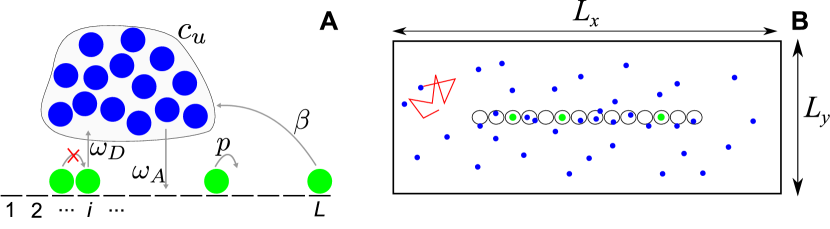
Figure 1: The two models studied in this work. Bound particles (in green) proceed along a filament with rate $p$, provided that the following site of the unidimensional lattice is empty; they are injected with rate $\omega_{\rm A}=\tilde{\omega}_{\rm A}c_{u}$ from a reservoir of unbound particles (in blue) with concentration $c_{u}$. Particles can then detach with rate $\omega_{D}$ on any site, and with rate $\beta$ on the last site. The total number of particles $N$ in the combined system of reservoir and filament is conserved. In panel (A) we depict the TASEP-LK_m model, with a spatially unstructured (i.e., homogenous) reservoir, while in the panel (B) we show a spatially extended reservoir of dimension $L_{x}\times L_{y}$ with closed boundary conditions. We explicitly consider the free diffusion of particles in it (a schematic trajectory of an individual particle is drawn in red). The sites of the filament have a finite extension modelled by disks playing the role of reaction volumes where particles can attach or detach. Note that a particle can diffuse within a reaction volume without attaching.

To study the depletion effects we define here two distinct models as sketched in figure 1: the first model considers an exclusion process in a finite homogeneous reservoir while the second model considers an exclusion process in a diffusive reservoir. The first model is an extension of the works [15, 16, 28] for homogeneous finite reservoirs, while the second one bears many similarities with the models with diffusive reservoirs as studied in, e.g., [17, 18, 19, 20, 21, 22].

2.1 Active motion of particles on the filament

One common way to address the formation of processive motor jams on filaments is to consider unidimensional driven lattice gases with steric interactions, namely exclusion processes [29, 30, 31].

The active motion of particles along the filament, as well as their exchange with the surrounding reservoir, is here formulated as a unidirectional exclusion process with Langmuir kinetics [15, 16, 28]. We in fact consider that motor protein transport is a continuous time Markovian hopping process of particles moving unidirectionally along a one-dimensional lattice at rate $p$, see figure 1 (A). The lattice has size $L$ with its sites labeled by $i=1..L$. The particles obey exclusion interactions implying that only one particle can occupy a single lattice site. Particles represent, for instance, the kinesin-8 motors, and their binding sites (the lattice sites) correspond to the tubulin dimers forming the microtubule. Just as kinesins on cytoskeletal filaments, particles in our models hop uni-directionally on the filament. Particles also attach to and detach from filament binding sites at, respectively, rates $\omega_{A}$ and $\omega_{D}$. The attachment-detachment process is therefore described by a Langmuir adsorption model [32]. Both directed transport and Langmuir kinetics respect the particle exclusion on the filament. We furthermore consider that particles reaching the last site of the lattice can detach from it at a rate $\beta\neq\omega_{D}$. The different rates and notations of the model are also defined in figure 1.

A meaningful continuum limit keeps $\Omega_{A}\equiv\omega_{A}L/p$ and $\Omega_{D}\equiv\omega_{D}L/p\sim\mathcal{O}(1)$ constant for $L\rightarrow\infty$ [15, 16]. The latter scaling implies that particles cross on average a finite fraction of the filament before detaching. The fraction between the typical runlength $\ell$ of a single motor and the filament length $L\>a$ is $\Omega^{-1}_{D}$, with $a$ the site length. The quantity $\Omega_{D}$ is therefore a directly measurable parameter. The attachment rate $\omega_{A}(i)$ at the filament binding site $i$ depends on the concentration $c_{u}(i)$ of motors in the reservoir around the site $i$, i.e. $\omega_{A}(i)=\tilde{\omega}_{A}c_{u}(i)$, where the binding rate constant $\tilde{\omega}_{A}$ is a parameter to be determined experimentally. We further consider the dimensionless constants $K^{\infty}\equiv c\,\tilde{\omega}_{A}/\omega_{D}$ and $\kappa^{\infty}\equiv\mu\,\tilde{\omega}_{A}/\omega_{D}$ that are, respectively, the renormalized total concentrations of motor proteins and binding sites (e.g. the concentration of polymerized tubulin dimers). The finite resource parameter $m$ can then be written in terms of these concentrations as $m=K^{\infty}/\kappa^{\infty}$. We also define the Langmuir equilibrium density as $\rho^{\infty}_{L}\equiv K^{\infty}/(K^{\infty}+1)$ (a.k.a. the Langmuir adsorption isotherm [32]), and the rate constant $\Omega^{\infty}_{A}\equiv c\,\tilde{\omega}_{A}L/p=K^{\infty}\Omega_{D}$ that corresponds to $\Omega_{A}$ in the case of unlimited resources.

We now characterize the features of the reservoir and the dynamics of unbound motors in the two models.

2.2 Exclusion process in contact with a homogeneous finite reservoir (TASEP-LK_m)

In the TASEP-LK_m we consider a homogeneous concentration that equals the total concentration of unbound motors in the reservoir, i.e. $c_{u}(i)=c_{u}$. The reservoir adds no additional dynamical rules to the system and we can study the impact of motor protein depletion on the transport characteristics by using a simple one-dimensional lattice model.

In the TASEP-LK_m the motor reservoir is modelled as a box with a number $N_{u}$ of unbound particles. Every time a particle detaches from the filament, $N_{u}$ increases by one unit, while every time a particle from the box attaches to the filament, $N_{u}$ decreases by one unit. The concentration of particles in the reservoir is then given by $c_{u}=N_{u}/V$, with $V$ the volume of the reservoir, see figure 1 (A). In this way the number of particles in the box determines the attachment rate on the lattice, and the dynamics on the lattice is thus coupled with the number of particles in the box.

Since the total number of motor proteins $N$ is limited (i.e. $N_{u}$ is finite), the rescaled concentration of unbound (or free) motors in the reservoir $K\equiv c_{u}\,\tilde{\omega}_{\rm A}/\omega_{\rm D}$ will in general be different to the total rescaled concentration of motors $K^{\infty}$. Indeed the balance between unbound and bound motors is given by total particle conservation $N=N_{u}+N_{b}$, with $N_{b}$ the number of particles attached to the filament. When this particle conservation equation is multiplied by $\tilde{\omega}_{\rm A}/(\omega_{\rm D}V)$, we get:

$$K^{\infty}=K+\rho\kappa^{\infty},$$ (1)

with $\rho$ the average fraction of binding sites (on the filament) that are occupied by motors. We mostly refer to $\rho$ as the bound motor density. The previous equation can be rewritten as

$$1=\frac{K}{K^{\infty}}+\rho/m,$$

with $m=K^{\infty}/\kappa^{\infty}$ as previously defined. When $m\rightarrow\infty$, $K=K^{\infty}$ and we recover the TASEP-LK_∞ with unlimited resources as it has been studied in the previous works [15, 16, 28]. The TASEP-LK_m here introduced is studied in Section 3.

2.3 Exclusion process in contact with a diffusive reservoir

The model presented so far considers one filament in contact with a reservoir with a homogeneously distributed pool of particles. Implicitly, this means that once a binding/unbinding event occurs, particles diffuse instantaneously in the reservoir to distribute homogeneously, despite the active transport along the filament that pushes to generate particle gradients in the solution. In these conditions, the particle attachment rate can be assumed as constant for any binding site along the filament. However, for real systems, particle diffusion is not instantaneous and, in contrast to the previous scenario, steady-state gradients of particle concentrations can build up in the solution. In such a situation, one can no longer assume that the particle attachment rate is uniform along the filament.

The second model that we study aims to understand whether diffusion and concentration gradients have an impact on the finite resources framework we have introduced with the first model. As shown in figure 1 (B), we consider that unbound point-like particles diffuse with a diffusion coefficient $D$ in a two-dimensional box (of area $L_{x}\times L_{y}$). This two-dimensional rectangular reservoir is the simplest generalisation that considers a spatially extended reservoir of the model previously introduced. While it is possible to consider many different three-dimensional reservoirs and geometries, for example placing the filament in a cylinder, the qualitative influence of diffusion on the competition between resources is not expected to be different in these geometries. A quantification of the effects of reservoir geometry on motor transport is out of the scope of the present work. Moreover, at fixed concentrations, adding one dimension needs to be compensated by a corresponding increase of the number of particles, and therefore a significant increase of the computational time.

We consider that unbound particles do not interact with each other and their position $\vec{r}$ evolves according to a Brownian dynamics. The equation of motion is:

$$\frac{d\vec{r}}{dt}=\vec{\xi}(t)\,,$$ (2)

where $\vec{\xi}$ is a Gaussian random noise verifying :

$$\langle\xi_{a}(t)\rangle = 0\,,$$ (3)

$$\langle\xi_{a}(t)\xi_{b}(t^{\prime})\rangle = 2D\delta(t-t^{\prime})\delta_{a,b}\,,$$ (4)

where the indices $a$ and $b$ stand for the space components ($x$ and $y$ directions). In the simulations, $D=5\mu m^{2}s^{-1}$, which is the same order of magnitude as the diffusive constant of motor proteins [17, 21]. The other parameters such as the particle hopping rate and the size of the reservoir are set to the typical values of in vitro experiments [14] (see table 1 and D). The main difference between this simulation scheme and the one in the papers [17, 18, 19, 20, 21], is that particles in the reservoir diffuse in a continuous space (and not on a lattice).

An unbound particle can attach to the filament at a constant rate $k$ when it is located within the reaction volume of a site $i$ of the one-dimensional lattice (these are represented by disks in figure 1 (B)). Therefore, in presence of motor diffusion in the solution, for the reasons explained above, the attachment rate $\omega_{A}(i)=\tilde{\omega}_{A}c_{u}(i)$ depends on the position $i$ of the site, through the concentration $c_{u}(i)$ of unbound particles present in the reaction volume of the site $i$. Here $\tilde{\omega}_{A}$ is constant for each site, and it is related via $\tilde{\omega}_{A}=kv_{R}$ to the intrinsic attachment rate $k$ of a single particle and to the reaction volume $v_{R}$. Note that here $v_{R}$ has the physical dimension of a surface since the simulations are in two dimensions. Once attached to the filament, the particle dynamics on the lattice follows the same rules of a standard exclusion process with Langmuir kinetics (as previously explained in 2.1). We refer to D for a detailed explanation of the simulation scheme.

3 Results: mean field solutions and simulations for TASEP-LK_m

We now develop an analytical theory for the stationary density profile of bound motors and their dependence on the limited number of motor proteins in the reservoir (i.e. resources). The TASEP-LK_m process in a finite reservoir, as defined in section 2.2, has four control parameters: the end dissociation rate $\beta/p$, the processivity parameter $\Omega_{\rm D}$, the total concentration of motor proteins $K^{\infty}$, and the concentration of tubulin dimers $\kappa^{\infty}$. These control parameters determine two stationary variables: the density profile of bound motors on the segment $\rho(x)$ and the concentration of unbound motors $K=c_{u}\,\tilde{\omega}_{\rm A}/\omega_{\rm D}$. The density profile $\rho(x)$ is defined as the continuum limit of the discrete profile $\rho_{i}$, with $i=1..L$ and correspondingly $x\in[0,1]$. Note that the continuum limit corresponds to $L\to\infty$, at fixed value of $m$, so that the number of particles increases accordingly, i.e. $N\to\infty$. The link between the profiles $\rho_{i}$ and $\rho(x)$ is given by $x=i/L$, and the stationary current is given by $J(x)=p\rho(x)(1-\rho(x))$. Note that in general $\rho_{L}\neq\lim_{x\rightarrow 1}\rho(x)$ for $L\rightarrow\infty$ due to the presence of a boundary layer of finite size (apart from the maximal current phase). We will also write $\rho\equiv\int^{1}_{0}dx\rho(x)$ for the average density. To determine the stationary value of $\rho(x)$ and $K$ we consider a set of three coupled equations determining the essential physics of the model.

The first one expresses the particle conservation, see equation (1):

$$K^{\infty}=K+\rho\>\kappa^{\infty}.$$ (5)

The finite resource parameter defined by $m=K^{\infty}/\kappa^{\infty}$ determines how much $K$ will differ from $K^{\infty}$, and thus how much the reservoir is depleted by the presence of the filament.

The second equation represents the balance of currents between the reservoir and the filament: in the stationary state the total current flowing from the reservoir to the filament is exactly balanced by the current flowing from the latter to the reservoir. We get the balance equation:

$$J_{\rm A}-J_{\rm D}-J_{\rm end}=0,$$ (6)

with the attachment current $J_{\rm A}/p=\Omega_{\rm A}(1-\rho)$, the detachment current $J_{\rm D}/p=\Omega_{\rm D}\>\rho$ and the end-dissociation current $J_{\rm end}/p=[1-\rho(1)]\rho(1)=(\beta/p)\>\rho_{i=L}$ . The current balance equation (6) can be solved for $\rho$,

$$\rho = \frac{K-(1-\rho(1))\rho(1)/\Omega_{\rm D}}{1+K}.$$ (7)

The third equation describes the stationary directed transport process of motors along the filament. In the continuum limit and in the stationary state, the equation for the density profile of bound motor proteins $\rho(x)$ writes generically as

$$\partial_{x}j(x)=\Omega_{D}\left\{K(1-\rho(x))-\rho(x)\right\}$$ (8)

where one can recognize the local balance between the current of active particles $j(x)$ and the local binding/unbinding events of the Langmuir kinetics $\Omega_{A}(1-\rho(x))$ and $\Omega_{D}\rho(x)$. For the totally asymmetric simple exclusion process the active current writes simply as $j(x)=\rho(x)(1-\rho(x))$. Note that this equation is actually a mean-field derivation of the TASEP-LK model where the relevant behavior occurs in the so-called “mesoscopic limit”, see for a detailed derivation and discussion [15, 16, 28].

We consider two solutions to the equation (8), a solution $\rho_{\alpha}$ with the boundary conditions $\rho_{\alpha}(0)=0$ and a solution $\rho_{\beta}$ with boundary condition $\rho_{\beta}(1)=1-\beta/p$. The analytical expression for the stationary profile $\rho(x)=\rho\left(x;K,\Omega_{\rm D},\beta/p\right)$ follows by selecting the solution with the minimal current [15, 16, 33]. Here we shortly present the qualitative results for $\rho(x)$, while the corresponding analytical expressions can be found in A.

As in the TASEP-LK_∞, the density profile $\rho(x)$ is characterized by four different phases: the low-density spike phase (LDs), the low-density no jam phase (LDn), the low density-high density coexistence phase (LD-HD) and the low density-maximal current coexistence phase (LD-MC). The LDs and LDn phases develop a continuous $\rho(x)$-profile at low average density $\rho<1/2$. The distinction between LDs and LDn is defined through the density value at the last site: in LDs the profile develops a spike at the last site $\rho_{L}>\rho(1)$ while in LDn the profile has no spike $\rho_{L}<\rho(1)$. Note that the notion of “spike” is related to that one of a “boundary layer” in exclusion processes. Both spikes and boundary layers characterize a significant deviation of the density profile at the filament end from the bulk profile given by the continuum limit equations. The main difference between both notions is that the spike relates to the average density on the last site while the boundary layer refers to the density profile over a finite characteristic length from the bulk towards the last site.

In the LD-HD and LD-MC phases the profile $\rho(x)$ develops a shock (or discontinuity) at $x=x_{w}$. Before the domain wall position (for $x<x_{w}$) we have a LD profile, while after domain wall position (for $x>x_{w}$) we have a HD or MC profile. These latter profiles are characterized by a high density $\rho>1/2$. The distinction between the HD and MC profile is that the former depends on the exit rate $\beta$ while the latter is independent of $\beta$ (see appendix A). The formation of a domain wall in the density profile corresponds to the onset of a queue of motor proteins on the filament, meaning that the filament is found in a coexistence of phases, with no jams before the domain wall and the queueing phase extending from the end of the filament.

To analytically determine the form of the density profile $\rho(x)$ and the concentration of free motors $K$ at finite resources, we have to solve the set of coupled equations (5), (7) and (8). In this respect, it is insightful to rewrite $K$ as a function of the current at the end tip $J_{\rm end}=p(1-\rho(1))\rho(1)$:

$$2K = -\left[1+\kappa^{\infty}(1-m)\right]$$ (9)

$$+\kappa^{\infty}\sqrt{\left(\frac{1}{\kappa^{\infty}}+1-m\right)^{2}+\frac{4}{\kappa^{\infty}}\left[m+(1-\rho(1))\rho(1)/\Omega_{\rm D}\right]}\;,$$

while $\rho$ as a function of $J_{\rm end}$ is given in equation (7). Equation (9) gives us readily the reservoir density in the LD-HD and LD-MC phases where the right boundary is fixed to $\rho(1)=\rho_{\beta}(1)=(1-\beta/p)$ and therefore $\rho(1)$ is independent from $\rho$ and $K$. We have then that $\rho(1)=1-\beta^{\ast}=1-{\rm min}\left\{\beta/p,1/2\right\}$ and we get the explicit expression for the rescaled reservoir density $K$ in the LD-HD and LD-MC phases:

$$2K = -\left[1+\kappa^{\infty}(1-m)\right]$$ (10)

$$+\kappa^{\infty}\sqrt{\left(\frac{1}{\kappa^{\infty}}+1-m\right)^{2}+\frac{4}{\kappa^{\infty}}\left[m+(1-\beta^{\ast})\beta^{\ast}/\Omega_{\rm D}\right]}.$$

When the filament is in the LD phase we do not have such an explicit expression for $\rho(1)$ that is no longer independent of $K$, and we are lead to solve an implicit equation on $K$. As discussed in detail in A, it is possible to write an expression for $\rho(1)$ as a function of $K$; plugging this expression into equation (9) then provides for the implicit solution equation. This approach can be developed also in presence of a finite homogeneous reservoir with excluded volume interactions between particles, see section 3.1.

We now present the results of the mean field framework presented in this subsection: first we discuss the depletion effects of the reservoir as a function of the finite resource parameter $m$, and then we show how finite resources affect the formation of jams; finally we present the novel phase diagrams obtained for various values of $m$.

3.1 Depletion of the reservoir

In figure 2 we have plotted the ratio $K/K^{\infty}$, between the motor concentration in the reservoir with respect to their total concentration, and the density of bound particles $\rho$ as a function of the finite resource parameter $m$. In particular, these curves can be interpreted as varying the number of motors $K^{\infty}$ while keeping the concentration $\kappa^{\infty}$ of tubulin dimers fixed, or reversely varying the concentration of tubulin dimers while keeping the concentration of motors fixed.

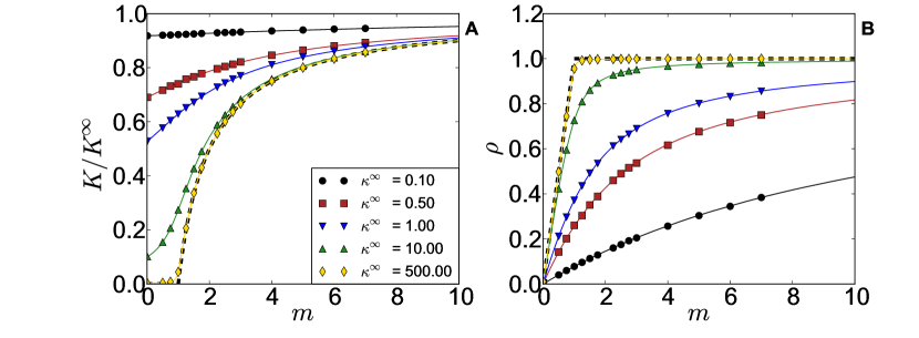
Figure 2: The depletion of particles in the reservoir $K/K^{\infty}$ (A) and the filling of the segments $\rho$ (B) as a function of $m$ for given values of $\kappa^{\infty}$, with $\Omega_{\rm D}=10$ and $\beta/p=0.8$. Solid lines are analytic expressions from mean field, Eqs. (7) and (9), and symbols are obtained from numerical simulations (see D for details). The black dashed line (which is almost superimposed by the yellow line with diamond markers) represents the limit $\kappa^{\infty}\rightarrow\infty$ of Eqs.(13) and (16).

We observe how the depletion of motors from the reservoir becomes relevant for small $m$ and large tubulin dimer concentrations (figure 2 (A)). Indeed, for an infinitely large reservoir we should have that $K^{\infty}=K$ while for small values of $m$ we get a $K\ll K^{\infty}$ indicating the depletion of the reservoir. Depleting the reservoir leads as well to a smaller density of bound motors since the stationary attachment rate decreases.

At constant $m$, in the limit of abundant binding sites and high motor concentrations we can analytically characterize the depletion effects. In the asymptotic limit, at which the motor protein concentration $K^{\infty}$ and the concentration of binding sites $\kappa^{\infty}$ are infinitely large, we find

$$\lim_{\kappa^{\infty}\rightarrow\infty}\frac{K}{K^{\infty}}=\left\{\begin{array}[]{ccc}0&&m\leq m_{c}=1\,,\\ (m-1)/m&&m>m_{c}=1\,,\end{array}\right.$$ (13)

$$\lim_{\kappa^{\infty}\rightarrow\infty}\rho=\left\{\begin{array}[]{ccc}m&&m\leq m_{c}=1\,,\\ 1&&m>m_{c}=1\,.\end{array}\right.$$ (16)

Interestingly, we recover a continuous phase transition in the reservoir consumption $K/K^{\infty}$. At very high levels of tubulin dimer concentrations, the reservoir is strongly depleted for values of $m$ smaller than $m_{c}=1$. By increasing $m<m_{c}$, most of the particles introduced into the system will add to the density of bound particles $\rho$, which thus increases linearly with $m$ until it eventually saturates and the filament is almost completely filled (see the yellow line with diamond markers in figure 2 (B)).

Equation (13) implies that $K$ will have a finite value for $m<m_{c}$, while it becomes infinite large for $m\geq m_{c}$. The transition at $m=m_{c}$ can by characterized by a change in the algebraic behaviour of the motor protein concentration $K$ in the reservoir as a function of the concentration of binding sites $\kappa_{\infty}$, viz. :

$$K=\left\{\begin{array}[]{ccc}\frac{m}{1-m}\left(1+\frac{\rho(1)(1-\rho(1))}{m\Omega_{D}}\right)+\mathcal{O}\left[\left(\kappa^{\infty}\right)^{-1}\right]&&m<m_{c}\,,\\ m\sqrt{\kappa_{\infty}}\left(\sqrt{1+(1-\rho(1))\rho(1)/\Omega_{\rm D}}\right)+\mathcal{O}\left[1\right]&&m=m_{c}=1\,,\\ (m-1)\kappa_{\infty}+\mathcal{O}\left[1\right]&&m>m_{c}\,.\end{array}\right.$$ (20)

We thus have for high values of $\kappa_{\infty}$ that the motor protein concentration in the reservoir converges to the finite value $m/(1-m)\left(1+\frac{\rho(1)(1-\rho(1))}{m\Omega_{D}}\right)$ for $m<m_{c}$, while it increases proportionally to the binding site concentration $\kappa_{\infty}$ for $m>m_{c}$. For values $m=m_{c}$ the motor protein concentration increases as a square root of $\kappa_{\infty}$.

As it will become clear in the next subsection, by measurements of the concentration of motors $K$, it is possible to determine the stationary density and current of the filament. Moreover, here we suggest that the motor protein density on a filament and its dependence on the reservoir concentration can depend on the local level of filament crowding (i.e. with different $\kappa^{\infty}$). This suggests that distinct parts of the cytoskeleton with locally different levels of filament crowding can potentially show rather different transport characteristics. This aspect is rationalized by the dependence of the derivative of the density, $\partial_{m}\rho$, see figure 2 (B). This derivative can strongly depend on $\kappa^{\infty}$, i.e. on the local concentration of potentially available binding sites. Interestingly, this argument can apply also to networks of filaments in contact with the finite reservoir of particles.

3.2 Density profiles by varying supply and demand

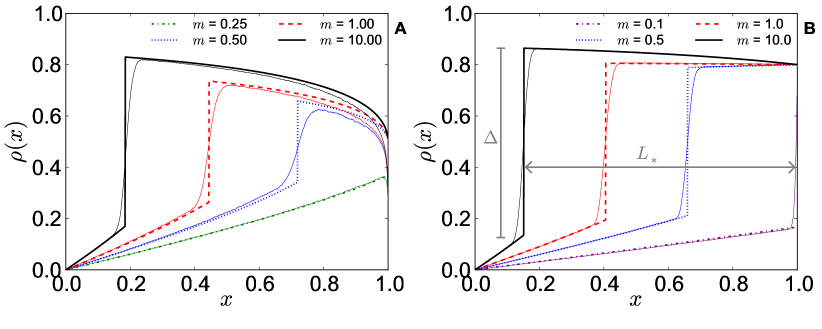
Figure 3: Density profiles for a TASEP-LK_m for different values of $m$ (see legend). In panel (A) we present a system with $\beta/p=0.8$, $\rho_{l}^{\infty}=0.9$ and $\Omega_{\rm D}=0.1$, moving from a LD-MC phase to a LDn phase when the resources become limiting (small $m$). Panel (B) shows the same system with $\beta/p=0.2$, with a LD-HD phase for large $m$ and a LDs for small $m$. Light lines are the outcome of numerical simulations with $L=1000$. We observe (not shown here) that the width of the domain wall becomes thinner as $L$ increases in the simulation results. We also indicate in the figure the domain wall height $\Delta$ and the domain wall distance from the filament end $L_{*}$.

Recall that the finite resource parameter $m$ indicates the number of motors in solution, relative to the number of polymerised tubulin dimers. In figure 3 we present the variation of the density profile $\rho(x)$ for given values of $\Omega_{\rm D}$, $\beta/p$ and total concentration of motors $K^{\infty}$ as a function of $m$. Decreasing $m$ reduces the observed density of processing motors on the filament, because less motors are available in solution. Thus the number of reservoir motors per binding site decreases.

With our approach we can also study the features of the motor protein jams. Figure 3 shows that a reduction of the resource parameter $m$ shifts the position of the domain wall to the right and thus decreases the jam length $L^{\ast}$ (the jam length is defined as $L_{\ast}=1-x_{w}$, with $x_{w}$ the domain wall position). This is an experimentally accessible quantity [14] that might be exploited to compare models and experimental outcomes. In figure 4 (A) we characterize the decrease of the jam length as a function of $m$. The jam length $L^{\ast}$ reaches zero length at a critical value of $m$ for which the system undergoes a phase transition from a LD-HD phase (or LD-MC) to a LDs (or LDn) phase. In figure 4 (B) we present the domain wall height $\Delta=1-2\rho(x_{w})$ as a function of $m$. Contrary to the the jam length $L_{\ast}$, the domain wall height $\Delta$ does not necessarily decrease as a function of $m$. Instead, we observe a different behaviour depending on whether the system is initially found in the LD-HD or LD-MC phase. In fact, the shock in the LD-MC disappears with a continuous transition in $\Delta$, while the shock in LD-HD disappears with a discontinuous transition in $\Delta$. So, whether the profile is in LD-HD or in LD-MC will determine its qualitative behaviour as a function of $m$.

Theory is compared to numerical simulations in figure 3; our analytical results are in good agreement with the simulations and the shock profile from the numerical simulations shows the expected finite-size effects. The slight disagreement between simulations and mean field solutions in the MC region is also present in the TASEP-LK_∞ [15, 16] and in TASEP [34, 35], and it is due to the divergence of the length scale of the boundary layer in the MC phase.

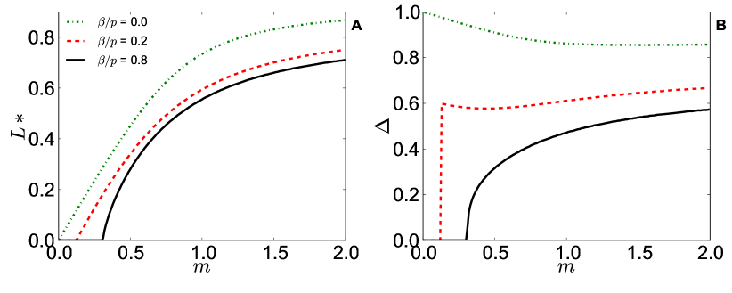
Figure 4: The jam length $L_{\ast}$ and domain wall height $\Delta$ are presented as a function of $m$ for $\rho^{\infty}_{\ell}=0.9$, $\Omega_{D}=0.1$ and given values of $\beta/p$. The curves are obtained from the mean field theory; black full lines denote a LD-MC to LDn transition, while the other curves show a LD-HD to LDs transition.

3.3 Phase diagrams at finite resources

In the previous subsection we have shown that by varying the parameter $m=K^{\infty}/\kappa^{\infty}$ we can induce phase transitions in the motor density profile on the filament. In this subsection we complement the picture by presenting how the phase diagram of TASEP-LK_m depends on the finite resource parameter $m$. Substituting the solution $K$ to the equations (7), (8) and (9) into the equations for the phase transition lines of TASEP-LK_∞ presented in A.2 determines such a phase diagram. Further detailed analysis is presented in B. Here we focus on the main results.

In figure 5 we present the $(\rho^{\infty}_{\ell},\beta/p)$ phase diagram for certain fixed conditions $(m,\Omega^{\infty}_{A})$. This type of phase diagram in the parameters $(\rho^{\infty}_{\ell},\beta/p)$ has been introduced in [14]. Upon decreasing $m$ the LDs phase gradually dominates the diagram and the LD-HD and LD-MC phase regions reduce in size. The LD-HD phase disappears only for $m\rightarrow 0$, whereas there exists a critical $m$ such that the LD-MC is no longer attainable (see B). Hence, when the motor resources are limited, the stationary density profiles are dominated by spikes. This is compatible with the behaviour shown in figure 3 (B): by decreasing $m$, the density profile exhibits signatures of a LDs. This result is also consistent with the limit $m\rightarrow 0$, corresponding to non-interacting isolated motors moving along the filament. Then the density profile is proportional to the residence time of the motors on the lattice dimers. In the $m\rightarrow 0$ limit, with filaments sparsely populated by motor proteins, our model reduces to the “antenna model” that has been considered in [13]. Due to the spike being located on the last site, this feature of the LDs might be important to regulate filament depolymerization by motor proteins [13, 36, 37, 38, 39]. In fact, the length-regulation of microtubule filaments is determined by the transit of motor proteins through their end tip and hence to the density at the end of the filament. It would therefore be interesting to study how the changes in the TASEP-LK phase diagram affects the depolymerization rate at finite resources, and hence if competition for resources can also determine the characteristic filament length.

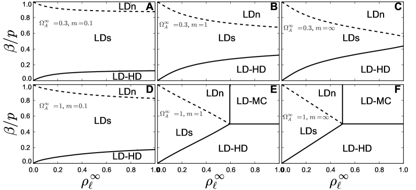
Figure 5: The $(\rho_{\ell}^{\infty},\beta/p)$-phase diagrams of TASEP-LK_m at given values of $\Omega^{\infty}_{A}$ and $m$. When $m$ becomes large we recover the phase diagrams presented in [14].

The diagrams in figure 5 also allow us to compare the present study with the results presented in the experimental work [14], where measured density profiles are interpreted using the revisited phase diagrams of TASEP-LK_∞. In particular, we have chosen $\Omega^{\infty}_{\rm A}=0.3$, as estimated in [14], to facilitate the comparison of our diagrams with the figures presented in [14]. We stress that, according to our estimates, $m\approx 10^{3}$ in [14] , meaning that the system is found in the infinite reservoir limit. If $m$ were reduced, e.g. by reducing the motor protein concentration while keeping the administered tubulin constant, we predict that the LDs phase would dominate the resulting experimental profiles. To check this, we suggest to repeat the assay [14], moreover reducing the employed motor protein concentration to approximately $1pM$.

An alternative way to represent the phase diagrams allows one to explicitly follow the development of phases as a function of the motor protein and tubulin concentrations in solution. In figure 6 we present such $(\kappa^{\infty},K^{\infty})$-phase diagrams at fixed $\Omega_{\rm D}$ and $\beta$, where the motor concentration $K^{\infty}$ and the concentration of polymerized tubulin dimers $\kappa^{\infty}$ are the employed control parameters. The latter gives rise to the possibility to fully sample the phase diagram [14] with the practical advantage that neither motor processivity nor end dissociation need to be controlled, e.g. by adjusting the solution’s salt concentration.

Tracing dot-dash lines in these $(\kappa^{\infty},K^{\infty})$ diagrams exhibits the system’s phase behaviour for a fixed value of $m=K^{\infty}/\kappa^{\infty}$. Importantly, that there is no direct way to pass from a LD-MC to an LDs phase. Thus, by decreasing the motor concentration $K^{\infty}$ the system will necessarily pass through the LDn phase. Starting from the LD-HD regime, the system can only undergo a transition to a LDs phase, see figure 6 panels (D-F). We also emphasize that the location of the transition lines depend only weakly on the processivity $\Omega_{D}$: between the first and last column of figure 6 the processivity varies by a factor $40$, without affecting the qualitative location of the transition lines.

These phase diagrams might hence be relevant in experimental scenarios like [14]. Since the total concentration of motors $K^{\infty}$ or of bound tubulin dimers $\kappa^{\infty}$ are controllable, these phase diagrams could allow for a quantitative interpretation of depletion effects on the observed density profiles. A typical feature appearing only at small $m$ is the predicted large extension of the LDs phase with respect to all phases. If the suggested experiments would manage to detect spikes in the motor density, one could hope for an accurate quantification of the prevalence of LDs over LD-HD and LDn.

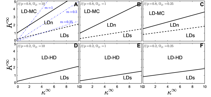
Figure 6: $(\kappa^{\infty},K^{\infty})$-phase diagrams for TASEP-LK_m at given values of $\Omega_{\rm D}$ and $\beta/p$. Thin dashed curves in panel (A) represent lines of constant $m$ ($m=0.25$, $0.5$, $1$).

3.4 Filaments without end dissociation rate

We end the analysis of the first model with the particular case for $\beta=0$ that allows us to derive some general model-independent results. In this case the current leaving the end of the tip is zero, and equations (5) and (7) decouple. The profile is in the LD-HD phase and the density at the end of the filament $\rho(1)=1$, is independent of the concentration of unbound motors $K$ (see A.2). We thus have $\rho=\rho_{\ell}\equiv K/(1+K)$, with a $K$ that follows readily by setting $\rho(1)(1-\rho(1))=0$ in equation (9). In the $\beta=0$ case, we recover the results presented by Klumpp and Lipowsky in [18]. This is not a coincidence, as both results are derived using the same two arguments: the total conservation of particles in the system and the balance of the currents between reservoir and filament. The results can be linked using a general formula we provide in C. The average density $\rho$ of bound motors for $\beta=0$ applies to a much larger class of transport processes than TASEP-LK_m (although the shape of the profile $\rho(x)$ is model dependent). Indeed, this is a direct consequence of the fact that when $\beta=0$ we do not need to consider the equation (8) for the steady-state density profile on the filament to solve equations (5-7) and the density on the filament is determined solely by the Langmuir adsorption process [32]. Consequently, our results remain valid for any other type of microscopic dynamic rule for the motor protein motion on the filament which does not correlate with the detachment/attachment process (such as bi-directional motion, for example) and they hold even for configurations with multiple filaments immersed in a homogeneous reservoir. For instance, the formalism proposed in this section is also valid for a network of cross-linked filaments or branched filaments. Moreover, the stationary density profile for a TASEP-LK_m on a network can be determined using the results [40, 41] and considering the appropriate value of $K$ (and thus $\rho$), as given by equations (7)-(9) when setting $\rho(1)=1$.

4 Simulation results for TASEP-LK in a diffusive reservoir

When not attached to a filament, motor proteins in a flow chamber or in the cytosol diffuse in solution with a presumed diffusion constant $D$. In stationary conditions, a gradient of motors is necessary to create the diffusive current balancing the current on the filament. By considering a diffusive reservoir, the motor concentration of particles $c_{u}(i)$ becomes a function of the site position $i$.

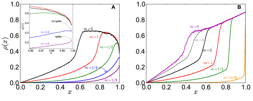
Figure 7: Density profile $\rho(x)$ obtained by explicitly considering the diffusion of particles in the reservoir. We have considered different values of $m$ starting from LD-MC (panel (A), $\rho_{\ell}^{\infty}=0.7$, $\beta/p=0.7$) and LD-HD (panel (B), $\rho_{\ell}^{\infty}=0.6$, $\beta/p=0.2$). In both panels we take $\Omega^{\infty}_{\rm A}=1$, $L=10^{3}$, the filament hopping rate $p=50s^{-1}$, the diffusion coefficient $D=5\mu m^{2}s^{-1}$, and the reaction volumes are modelled by spheres with diameter $a=10^{-2}\mu m$. The dimensions of the reservoir are $L_{y}=0.5\mu m$ and $L_{x}=100\mu m$. We observe the same phenomena as in TASEP-LK_m: for large $m$ there appears a domain wall in the system. In panel (A) there is a transition from LD-MC at $m=$1, 1/2 over LDn at $m=1/4$ to LDs at $m=1/8$. In panel (B), the system goes from LD-HD at $m=2$ to LDs for $m\lesssim 0.06$.

Here we show that a TASEP-LK with a diffusive reservoir exhibits the same phenomenology as a TASEP-LK_m without reservoir motor diffusion.

To this end, we perform numerical simulations of the model introduced in Section 2.3, providing a simplified and in silico version of the experiment presented in [14]. The details and the parameters of the employed simulation scheme can be found in D and in table 1, respectively.

Table 1: Parameters of the model with “diffusive“ reservoir: values estimated from in vitro experiments [13, 14] (if not otherwise specified) and values used in simulations throughout the paper. The last row shows the competition parameter $m$, which has been fixed to high values in in vitro experiments of kinesin transport along microtubules [14] to avoid depletion effects; here we can modulate the parameter $m$ to study the competition for resources.

• 		Typical values in
  		experimental conditions	Simulations
  $D$	Diffusion coefficient	$\approx 4~{}\mu m^{2}s^{-1}$ [17, 27]	$5~{}\mu m^{2}s^{-1}$
  $p$	Hopping rate	$1-100~{}s^{-1}$ [42]	$50~{}s^{-1}$
  $\beta/p$	Rescaled end-dissociation rate	$0.01-0.95$	$0.1-0.9$
  $a$	site length	$8~{}nm$	$10~{}nm$
  $L_{x,y}$	Reservoir edge-sizes	$\approx 10^{2}\mu m$	$L_{x}=12.5-200~{}\mu m$; $L_{y}=0.25-4~{}\mu m$
  $L$	Microtubule length	$\sim$250-1250 sites	1000 sites
  $\Omega_{A}^{\infty}$	Rescaled association ratea	$\sim 0.3-1$	$0.3-1$
  $\rho_{\ell}^{\infty}$	Langmuir densitya	$\sim 0.1-0.9$	$0.25-0.7$
  $m$	Competition parameter	$\gtrsim 1000$$~{}^{\rm b}$	$\sim 0-10$

• ^a To better emphasize that the range of values used in simulations is of the same order of magnitude of the experimental ones, in this table we have used $\Omega_{A}^{\infty}=c\,\tilde{\omega}_{A}L/p=K^{\infty}\Omega_{D}$ and $\rho_{\ell}^{\infty}=K^{\infty}/(K^{\infty}+1)=\Omega_{A}^{\infty}/(\Omega_{A}^{\infty}+\Omega_{D})$ defined in Section 2.1 as control parameters of the model.

• ^b Value estimated from [13, 14].

In figure 7-(A) we show an LD-MC density profile whereas in figure 7-(B) we show an LD-HD density profile that are obtained by model simulations for various ratios $m$. As observed in TASEP-LK_m, the position of the domain wall is strongly affected by changing the competition parameter $m$. Decreasing the value of $m$ leads to a gradual shift in the domain wall towards the end of the lattice. In panel (A), starting from an LD-MC profile and decreasing $m$, the system undergoes first a transition to a LDn profile without spike and eventually to a LDs profile with a spike, see the inset of figure 7-(A). This is an interesting and prominent feature predicted by the TASEP-LK_m phase diagram from figure 6. Since experiments can detect the appearance of spikes, the domain wall dependence on controllable parameters allows for an experimental validation of the models studied. In panel (B), starting from the LD-HD phase and decreasing $m$, the domain wall disappears and the profiles display the signature of LDs with a spike at the end of the filament, see $m=0.06$ in figure 7 (B). Moreover, in the panels of figure 7 we observe a dependency of the length $L_{*}$ and the height $\Delta$ of the shock on the supply-demand parameter $m$ that is in agreement with the one noticed in the TASEP-LK_m, see figures 3 and 4. By decreasing $m$, the length $L_{*}$ of the jam decreases and the height $\Delta$ goes abruptly to zero (leading to a spike) or smoothly to zero when starting from the LD-HD or LD-MC respectively.

These results show the robustness of the observations made for TASEP-LK_m: the presence of diffusion and motor concentration gradients does not affect the qualitative features of the transitions from LD-MC to LDn and from LD-HD to LDs.

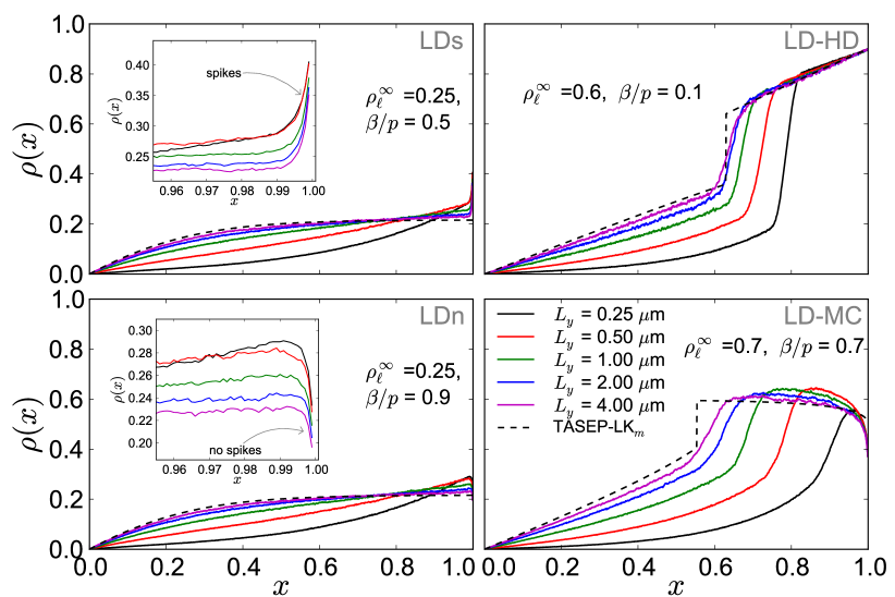
Figure 8: Density profile of motors along the filament for the TASEP-LK in a reservoir with diffusive particles. The different panels correspond to the phases explained in figure 5, and in particular panel (E). When the section $L_{y}$ of the reservoir is increased (from 0.25 to 4.00 $\mu$m) we observe the convergence of the profiles to the mean field value expected for the TASEP-LK_m (dashed line). This corresponds to a concentration gradient along the longitudinal direction of the filament that becomes negligible (not shown). We kept hereby the volume $L_{x}\cdot L_{y}=50\mu m^{2}$ fixed and left all the other parameters unchanged. In the insets of the left panel we magnify the region close to the end of the filament to emphasize the presence of spikes (LDs) or their absence (LDn). All the figures have $\Omega^{\infty}_{\rm A}=1$, $m=1$, $L=10^{3}$, the hopping rate on the filament $p=50s^{-1}$, the diameter of the site reaction volume is $a=10^{-2}\mu m$, $c=3.32\cdot 10^{-11}mol\,m^{-2}$ and $D=5\mu m^{2}s^{-1}$.

In figure 8 we show that, remarkably, the exclusion model with diffusion converges to the analytical solutions of the TASEP-LK_m under certain conditions. In particular, we have checked the effects of reservoir size on the density profile on the filament. As we show in figure 8, when the cross-section $L_{y}$ of the reservoir increases, the density profile converges toward the mean field prediction of the TASEP-LK_m. This has an intuitive explanation: in a closed compartment, the diffusive motor current passing through a surface perpendicular to the filament counterbalances the opposite active current along the filament. As explained below, the diffusive current is proportional to both the cross-section and the gradient of particles in the reservoir. Accordingly, increasing $L_{y}$ will decrease the concentration gradient.

More specifically, the current of motors $J_{f}$ on the filament is in general not homogeneous for the TASEP-LK, and depends on the position $x$ i.e. $J_{f}=J_{f}(x)$. The opposite current $J_{r}$ in the reservoir is related to the concentration gradient $\vec{\nabla}c(x,y)$, where the concentration is now a function of the position in the plane $(x,y)$. We have checked numerically for the largest edge-size in the $y$ direction ($L_{y}\sim 4\mu m$) that the concentration of particles is homogeneous along the $y$ direction. Homogeneity for the parameters considered is thus expected to hold as well at smaller edge-sizes $L_{y}$. Therefore we can assume that the concentration is homogeneous along the y-direction i.e. $c(x;y)=c(x)$. The same reasoning would hold for a third spatial dimension $z$.

The diffusive current in the reservoir reads $J_{r}(x)=-DL_{y}\,dc(x)/dx$. Balancing the currents $J_{f}(x)=J_{r}(x)$ at position $x$ implies:

$$J_{f}(x) = DL_{y}\frac{dc(x)}{dx}\,.$$

This equation tells us that, for a given (upper bounded) current on the filament, the gradient vanishes upon an increase of the cross-section $L_{y}$. For the largest cross section $L_{y}=4\mu m$, the motor gradients is typically $16$ times smaller as compared to the smallest cross section $L_{y}=0.25\mu m$. Hence the finite diffusion in the reservoir is counterbalanced by appropriate dimensions of the reservoir. Thus, elongated reservoir cross section favour homogeneity of supply motors. For this reason, the solutions of the TASEP-LK_m can provide a good approximation of the system when the cross section of the reservoir is large enough (see figure 8). Hence, we have shown that in some geometries the reservoir is approximately homogeneous and we quantitatively recover, as expected, the results previously presented for the TASEP-LK_m.

5 Discussion

We have introduced a theoretical framework to investigate the regulatory effects of a finite closed reservoir of motor proteins on the formation of traffic jams on cytoskeletal filaments. In particular, we have studied two models with limited resources of motors and their binding sites. They represent finite processive motors moving along a filament in contact with a finite reservoir of motors, and describe how the emergence of traffic jams can be regulated by the supply-demand of molecular motors in the system. Our model can be seen as a generalization of exclusion processes with Langmuir kinetics and infinite resources indicated as TASEP-LK_∞ in the text [15, 16, 28]. In the present formulation we study the impact on transport characteristics of a limited reservoir of particles, as a possible experimental situation in in vitro and in vivo experiments, recovering previous results in some limiting cases. The competition for motor proteins is determined by the fraction $m$ between the total concentration of motor proteins and the concentration of binding sites (tubulin dimers).

The analytical solutions are confirmed by numerical simulations and they allow us to characterize the dependence between motor crowding phenomena and supply, thus leading to propose a novel determinant of traffic jams: the competition parameter $m$. Although the proposed theory can be far from real in vivo situations, it implies that in different regions of the cytoskeletal network the parameter $m$ can locally change according to inhomogeneities in motor protein and filament concentrations or, more in general, availability of binding sites in competition with other proteins binding to cytoskeletal filaments.

Our model predicts that the onset of jams and other motor traffic features can be determined by the local supply-demand constraint. For instance, depending on the local tubulin concentration, crowding phenomena set up differently upon changes in $m$. The simple supply-demand balance might then be relevant for traffic regulation inside the cell.

We have first analysed a system with a homogeneous distribution of particles in the reservoir (TASEP-LK_m, Section 3), for which we are able to provide analytical solutions. When the amount of motor proteins in the system is finite, there appears a pronounced depletion of the motor reservoir at small values of $m$ (figure 2). In this regime we have found strong competition of the binding sites for the relatively few motors in the system. We have shown that it is possible to devise quantitative relationships between the motor density on the filament and the total availability of resources. By measuring the concentration of free motors in the reservoir it is possible to extract information on the crowding of the filament. Interestingly, when either the amount of binding sites or the concentration of motors is large ($\kappa^{\infty}$ or $K^{\infty}$ tend to infinity) we found a critical behaviour. For values of $m<m_{c}$ we observe the very strong depletion of the reservoir for which most of the motors in the system are bound to the filament. Interestingly, in this regime, the concentration of motors in solution remains finite although its fraction with respect to the total concentration converges to zero. This is a subtle result since, even in the large $L$ limit (i.e. large $\kappa^{\infty}$), motors still dissociate from the filament. Accordingly, one would naively expect a finite fraction of motors in the solution.

We then map two different phase diagrams of the system: one as proposed in [14] with $\beta/p$ and $\rho_{\ell}^{\infty}$ as control parameters, the other with the rescaled total concentrations of tubulins and motors ($\kappa^{\infty}$ and $K^{\infty}$ respectively). We have investigated those phase diagrams at different supply-demand ratios $m$ and underlined the traffic effects introduced by the finite pool of motors. The $(\rho_{\ell}^{\infty},\beta/p)$ phase diagram is however difficult to reconstitute experimentally, since the corresponding parameters cannot be easily modified independently. Instead, the novel phase diagram introduced here allows to study the effects of limited resources in a straightforward way. By examining the phase diagrams it becomes apparent how the presence of a shock on the filament is affected by the limitation of resources: at low motor concentrations or high amount of cytoskeletal binding sites, the spike phase LDs dominates the $(\rho_{\ell}^{\infty},\beta/p)$ phase diagram. An LD-HD phase is always achievable, but it might only appear at the very low values of the end-dissociation rate $\beta$. Moreover, from the ($\kappa^{\infty}$, $K^{\infty}$) phase diagram it is evident that, starting from an LD-MC phase, the LDs phase can only be reached after a passage to the LDn phase, while starting from the LD-HD phase the LDn phase cannot be found. We find that the phase diagram of TASEP-LK_m interpolates between the antenna model neglecting excluded volume interactions and TASEP-LK_∞, with a phase diagram characterized by excluded volume interactions. The TASEP-LK_m model thus quantifies how excluded volume determines active motor protein transport.

The formalism developed for a single filament can be extended to more general cases and in particular to investigate a population of filaments, as has been done before for a multi-TASEP model with finite resources [25]. Nevertheless, the results we obtain for $\beta=0$ remain valid for any other type of motor dynamics on the segment, e.g. bi-directional motion, and for any configuration of filaments immersed in a homogeneous reservoir, as in a network of cross-linked or branched filaments mimicking a cytoskeleton, as studied in [40, 41].

In the section 4 we have considered a reservoir of diffusive particles in order to investigate the impact of diffusion and of concentration gradients on the TASEP-LK_m phenomenology. With finite diffusion the active transport indeed creates a stationary gradient of particles in the reservoir. The presence of such a gradient introduces spatial inhomogeneities in the motor-filament attachment rates. Numerical simulations in section 4 revealed an important coincidence of phase behaviour for these two distinct systems, namely (i) the TASEP-LK_m and (ii) TASEP-LK model with explicit motor diffusion. In particular, upon changing $m$, both domain wall and phase transition behaviour is qualitatively similar in both systems. Decoupling supply-demand effects and motor diffusion can therefore already provide a qualitative understanding of the main system features.

We stress that, although the two models are different, we can recover the TASEP-LK_m in certain limiting cases: in fact we have shown by numerical simulations, and explained with a theoretical argument, how the change of the reservoir geometry results in very similar outputs of the two models. By increasing the cross section of the reservoir, we observe the convergence of the motor density profile along the filament to the mean field prediction of the TASEP-LK_m. Therefore we expect our analytical theory to remain valid and provide quantitative good results when the reservoir is sufficiently large (as in many in vitro systems).

This work introduces an important parameter, the finite resources parameter $m$, describing the competition between the concentration of polymerized cytoskeletal filaments and the number of motors in solution, to the theoretical description of in vitro experiments as performed in [14]. Those experiments, indeed, have been done at very low concentration of tubulin (pM) with respect to the concentration of motors (nM). As a consequence, the system studied was in the infinite resource limit. With the TASEP-LK_m it is now also possible to study regimes for which the tubulin concentration is comparable to the motor protein concentration, and thus the competition between supply and demand of polymer binding sites for motors is relevant. The phase diagram in the ($\kappa^{\infty}$,$K^{\infty}$)-plane opens the possibility to tune directly the experimental setup (by changing the length of microtubule filaments and/or the concentration of motor proteins) and straightforwardly compare observed motor protein density profiles to our analytical theory. Although we are aware that the models proposed only constitute an approximation of in vivo systems, we can speculate that the motor density phenomenology presented qualitatively holds when and where the competition for motor proteins becomes relevant. For instance we notice that our modeling framework is consistent with in vivo experimental results [27]. In this work Blasius et al. have observed an exponential profile of kinesin-1 motors along the length of CAD cell neurites and hippocampal axons. We could qualitatively observe the same behaviour for systems in LD phases and small $m$ (see e.g. black line in the top left panel of Fig. 8), with characteristic lengths of the same order of magnitude of the one found in [27]. This is a promising signature for future applications of our model, but a more quantitative and careful investigation would require more information on the physiological parameters and it is however beyond our presentation.

Through the control of the crowding effects in the different phases, the competition for resources can also affect another important biological process, namely the length-regulation of the filament. In fact it is well known that the motion of motor proteins (e.g. kinesin-8 Kip3p) at the filament tip can regulate its depolymerization [13, 36, 37, 38, 39]. In this perspective, it would be interesting to study how the competition for resources regulates the filament depolymerization rate, and to relate filament length regulation to the phase diagrams of TASEP-LK_m that we have presented here. Note that to study the filament length regulation at finite resources it is also necessary to consider the concentration of tubulin dimers in the flow chamber solution/cytosol. Such a study is out of the scope of this paper.

Appendix A TASEP-LK_∞: density profiles and phase diagrams at infinite resources

We consider here the TASEP-LK_∞ model with with infinite resources suc that the the total motor concentration $c$ equals to the concentration of motors in the reservoir $c_{u}=c$. We have as well for the renormalized motor concentrations $K=K^{\infty}$ (with $K=\tilde{\omega}_{A}c_{u}/\omega_{D}$, and $K^{\infty}=\tilde{\omega}_{A}c/\omega_{D}$). The continuous density profile $\rho(x)$ for TASEP-LK_∞ follows from the solution of the continuum mean field equations [15, 16]:

$$\Omega^{-1}_{D}[2\rho(x)-1]\partial_{x}\rho(x)+K[1-\rho(x)]-\rho(x)=0\;,$$ (21)

with boundary conditions $\rho(x=1)=1-\beta$ and $\rho(x=0)=0$, where here and in the rest of this appendix we have posed, for the sake of simplicity and without loss of generality, $p=1$. In the following we write down the analytical expression for the density profile $\rho(x;K,\Omega_{\rm D},\beta)$ by solving equation (21), and present the corresponding phase diagram. We closely follow the procedure presented in [15, 16].

A.1 Density profile

We write the density profile in terms of the “renormalized” profile $\sigma\left(x\right)=\frac{K+1}{K-1}(2\rho(x)-1)-1$, where we have dropped the dependency on $K$, $\Omega_{\rm D}$ and $\beta$ for convenience. The renormalized profile $\sigma(x)$ can have three different forms determining the phase of the system. The system presents a low density phase (LD) where the density profile is continuous, a low density-high density coexistence phase (LD-HD) and a low density-maximal current coexistence phase (LD-MC) where the profile develops a shock at a position $x_{w}$ separating a low density region from a high density region (or a maximal current region). Here we make a further distinction among the LD phase, and we name LDn (no jam) a low density phase with no presence of jams at the end (as in the case shown in figure 3 (A) for small $m$). Instead, we name as LDs (spike) the low density phase with an occupation spike on the last site (as the profile with the smallest $m$ shown in figure 3 (B)).

The profile $\sigma(x)$ is thus given by:

• LD-phase: $\sigma(x)=\sigma_{L}(x)$

• LD-HD phase: $\sigma(x)=\left\{\begin{array}[]{ccc}\sigma_{L}(x)&&x<x_{w}\\ \sigma_{R}(x)&&x>x_{w}\end{array}\right.$

• LD-MC phase: $\sigma(x)=\left\{\begin{array}[]{ccc}\sigma_{L}(x)&&x<x_{w}\\ \sigma_{MC}(x)&&x>x_{w}\end{array}\right.$

with $\sigma_{L}$ the left boundary solution (for which $\rho_{\alpha}(0)=0$), $\sigma_{R}$ the right boundary solution (for which $\rho_{\beta}(1)=1-\beta$) and $\sigma_{MC}$ the saturated maximal current solution (for which $\rho_{MC}(1)=1/2$). The point $x_{w}$ is defined by the equation $\sigma_{L}(x_{w})+\sigma_{R}(x_{w})=-2$ or equivalently $\rho_{\alpha}(x_{w})=1-\rho_{\beta}(x_{w})$. The left and right boundary solutions are given in terms of the real valued branches $W_{0}$ and $W_{-1}$ of the Lambert-W function [43]. We have for the expression of $\sigma_{L}$

$$\sigma_{L}\left(x\right)=\left\{\begin{array}[]{ccc}W_{0}\left(\frac{2K}{1-K}\exp\left(\Omega_{\rm D}\frac{(K+1)^{2}}{K-1}x-\frac{2K}{K-1}\right)\right)&&K<1\\ W_{-1}\left(\frac{2K}{1-K}\exp\left(\Omega_{\rm D}\frac{(K+1)^{2}}{K-1}x-\frac{2K}{K-1}\right)\right)&&K>1\end{array}\right.,$$ (24)

and the right boundary solution $\sigma_{R}$ is given by

$$\sigma_{R}(x)=\left\{\begin{array}[]{ccc}W_{-1}\left(\left(\frac{K+1}{K-1}(1-2\beta)-1\right)\exp\left(\Omega_{\rm D}\frac{(K+1)^{2}}{K-1}(x-1)+\left(\frac{K+1}{K-1}(1-2\beta)-1\right)\right)\right)&&K<1\\ W_{0}\left(\left(\frac{K+1}{K-1}(1-2\beta)-1\right)\exp\left(\Omega_{\rm D}\frac{(K+1)^{2}}{K-1}(x-1)+\left(\frac{K+1}{K-1}(1-2\beta)-1\right)\right)\right)&&K>1\end{array}\right..$$ (27)

(28)

Figure 9: The $(\rho_{\ell}^{\infty},\beta)$-phase diagrams for TASEP-LK_∞ for given values of $\Omega_{\rm D}$.

A.2 Phase diagram for infinite resources

We now determine the $(\rho^{\infty}_{\ell},\beta)$-phase diagram at infinite resources for fixed values of $\Omega_{\rm D}$. In this case we have $K=K^{\infty}$ and therefore $\rho^{\infty}_{\ell}=K/(K+1)$. We get the following equations for the transitions between the LDs, LDn, LD-HD and LD-MC phases:

• LD-HD to LD-MC: the transition happens at $\beta=1/2$ for $K>1$.

• LD-HD to LDs: this transition occurs for $\beta<1/2$. The transition is given by the condition $\rho_{\alpha}(x=1)=1-\rho_{\beta}(x=1)=\beta$. Note that this condition corresponds to $\rho_{\alpha}(x=1)(1-\rho_{\alpha}(x=1))=\beta(1-\beta)$, or, setting the current to the left of the shock equal to the current leaving the segment. From the solution for $\rho_{\alpha}$, which follows from equation (24), we find, for the critical $\beta<1/2$:

  $$\beta=\left\{\begin{array}[]{ccc}\left(\frac{K-1}{2(K+1)}\right)W_{0}\left(\left|\frac{2K}{K-1}\right|\exp\left(\Omega_{\rm D}\frac{(K+1)^{2}}{K-1}-\frac{2K}{K-1}\right)\right)+\frac{K}{K+1}&&K<1\;,\\ \left(\frac{K-1}{2(K+1)}\right)W_{-1}\left(-\left|\frac{2K}{K-1}\right|\exp\left(\Omega_{\rm D}\frac{(K+1)^{2}}{K-1}-\frac{2K}{K-1}\right)\right)+\frac{K}{K+1}&&K>1\;.\end{array}\right.$$ (31)

  (32)

• LDn to LD-MC: this transition happens at the critical $K_{c}>1$ at which $\beta_{c}=1/2$ in equation (32). Hence, we get the equation

  $$\left\{\begin{array}[]{ccc}W_{0}\left(\left|\frac{2K}{K-1}\right|\exp\left(\Omega_{\rm D}\frac{(K+1)^{2}}{K-1}-\frac{2K}{K-1}\right)\right)=-1&&K\leq 1\;,\\ W_{-1}\left(-\left|\frac{2K}{K-1}\right|\exp\left(\Omega_{\rm D}\frac{(K+1)^{2}}{K-1}-\frac{2K}{K-1}\right)\right)=-1&&K\geq 1\;,\end{array}\right.$$ (35)

  which provide the transition lines for values of $\beta>1/2$. We can now use that $W_{0}(-1/e)=W_{-1}(-1/e)=-1$, to obtain the result

  $$\begin{array}[]{ccccccc}\Omega_{\rm D}&=&&\frac{1}{K+1}+\frac{(K-1)}{(K+1)^{2}}\ln\left(\frac{K-1}{2K}\right)&&&\Omega_{\rm D}<0.5\;,\\ K&=&1&&&&\Omega_{\rm D}>0.5\;.\end{array}$$ (38)

• LDs to LDn: this transition is given by the condition $\rho_{\alpha}(x=1)=\rho_{i=L}$. Since, $\beta\rho_{i=L}=\rho_{\alpha}(x=1)(1-\rho_{\alpha}(x=1))$ we get the condition $\rho_{\alpha}(x=1)=1-\beta$. We thus see that when $\beta_{c}$ is the transition from LD-HD to LDs, then $1-\beta_{c}$ denotes the transition from LDs to LDn.

In figure 9 we have drawn the corresponding $(\rho^{\infty}_{\ell},\beta)$-phase diagrams for the TASEP-LK_∞.

Appendix B TASEP-LK_m: Phase transition lines for finite resources

To get the phase diagrams for the TASEP-LK_m at finite resources we are led to substitute the concentration of motors at finite resources $K(\beta,\Omega_{\rm D},\kappa^{\infty},K^{\infty})$, (solution of the equations (7), (8) and (9)) into the equations for the phase transitions at infinite resources (found in A.2).

Below we present the analytical results obtained for the phase transition lines:

• LD-HD to LD-MC: the critical transition line is given by:

  $$\beta = 1/2\ \ {\rm for}\ \ K(\beta,\Omega_{\rm D},\kappa^{\infty},K^{\infty})>1\;.$$ (39)

• LD-HD to LDs: The critical value $\beta_{c}$ follows from solving an implicit equation that we find from the substitution of $K(\beta,\Omega_{\rm D},\kappa^{\infty},K^{\infty})$ into the equation (32). For instance, when $\Omega_{\rm D}\rightarrow\infty$, from Eq. (7) the density on the lattice corresponds to the one that would be obtained in a closed system: $\rho=\rho_{\ell}=K/(K+1)$. From that we get the critical beta $\beta_{c}=K/(K+1)$.

• LDn to LD-MC: We substitute the stationary value of $K(\beta=1/2,\Omega_{\rm D},\kappa^{\infty},K^{\infty})=K^{\ast}$, which follows from setting $\rho(1)=1/2$ in equation (9), into the equation (38). We then have, for $\beta>1/2$, the solution

  $$\begin{array}[]{ccccc}\Omega_{\rm D}&=&\frac{1}{K^{\ast}+1}+\frac{(K^{\ast}-1)}{(K^{\ast}+1)^{2}}\ln\left(\frac{K^{\ast}-1}{2K^{\ast}}\right)&&\Omega_{\rm D}<0.5\;,\\ K^{\ast}&=&1&&\Omega_{\rm D}>0.5\;.\end{array}$$ (42)

• LDs to LDn: If $\beta_{c}$ denotes the LDs to LD-HD transition, then $1-\beta_{c}$ denotes again the transition from LDs to LDn. Indeed, the transition from LDs to LD-HD is denoted by the condition $\rho_{\alpha}(x=1;K,\Omega_{\rm D})=\beta$ and the transition from LDs to LDn by $\rho_{\alpha}(x=1;K,\Omega_{\rm D})=1-\beta$. For finite resources, $K\neq K^{\infty}$ is a function of $\beta$ itself. However, the dependency of $K$ on $\beta$ is given by the current at the end tip $\rho(x=1)(1-\rho(x=1))=\beta(1-\beta)$, which is independent of the transformation $\beta\rightarrow 1-\beta$. Hence, also for finite resources, the critical transition $\beta_{c}$ from LDs to LDn is given by $1-\beta_{c}$ the transition of LDs to LD-HD.

Let us finally present some formal analytical result on the nature of the phase diagrams in figure 5. We see that when $m$ becomes smaller the LD-MC phase and LD-HD phase reduce in size and the LDs phase becomes more prominent. While the LD-HD phase will only disappear for $m\rightarrow 0$, the LD-MC phase will disappear for some $m=m^{\ast}>0$. To find this “critical” $m^{\ast}$ we set $\rho_{\ell}=1$ in equation (42) to find for $\Omega_{\rm D}>1/2$, or equivalently $m\in[1/4,1/2]$:

$$m^{\ast} = \frac{1}{2}\left(1-\frac{1}{4\Omega_{\rm D}}\right)\;,$$ (43)

while for $\Omega_{\rm D}<1/2$ and thus $m<1/4$ we need to solve

$$\frac{1+4\Omega_{\rm D}}{4(1-m^{\ast})}=1+\frac{4(2m^{\ast}-1)\Omega_{\rm D}+1}{1+4\Omega_{\rm D}}\ln\left(\frac{4(2m^{\ast}-1)\Omega_{\rm D}+1}{2(4m^{\ast}\Omega_{\rm D}+1)}\right)\;.$$ (44)

Appendix C TASEP-LK: Reservoir with excluded volume

Let us consider a reservoir in which particles feel in the reservoir an exclusion interaction. A formula for the bound density has then been derived in [18] (compare equation (3) in [18] with equations (4) and (6) in this work). We now show the connection between these equations.

Our results can be easily generalized to the case of a finite reservoir with exclusion interactions. To define such a reservoir, we have to consider particles with a finite volume $v_{m}$, leading to the fraction $\phi_{u}=c_{u}v_{m}$ of the volume being occupied. Hereby we have assumed that the filament itself has no volume (but this can be easily corrected when renormalizing the volume).

The equation for the mass conservation (5) and the hydrodynamic equation for the bound density (7) remain the same. What does change with volume exclusion is the balance between reservoir and segment. In fact, the detachment current will now be $J_{D}=\omega_{\rm D}\rho(1-\phi_{u})$, and the exit current $J_{\rm end}=\rho(1)[1-\rho(1)]=\beta(1-\phi_{u})\rho_{i=L}$. We recover the result without exclusion $J_{D}=\omega_{\rm D}\rho$ when $v_{m}\rightarrow 0$ or equivalently $\phi_{u}\rightarrow 0$. The balance equation becomes then

$$\rho=\frac{K-\Omega^{-1}_{D}[1-\rho(1)]\rho(1)}{K+(1-\phi_{u})}.$$ (45)

It is useful to write $\phi_{u}=K\left(v_{m}\omega_{\rm D}/\tilde{\omega}_{A}\right)$. Accordingly $K$ is again function of $\rho(1)$:

$$2\left(1-v_{m}\omega_{\rm D}/\tilde{\omega_{\rm A}}\right)K=-1-Q$$

$$+\sqrt{1+Q^{2}+4\>\left(1-v_{m}\omega_{\rm D}/\tilde{\omega_{\rm A}}\right)\left\{K^{\infty}+\kappa^{\infty}[1-\rho(1)]\rho(1)/\Omega_{\rm D}\right\}},$$

(46)

with

$$Q=\kappa^{\infty}-\left(1-v_{m}\omega_{\rm D}/\tilde{\omega_{\rm A}}\right)K^{\infty}.$$ (47)

It is interesting to notice that in the case $\beta=0$ we recover the formula (3) present in [18] when setting $v_{m}=1$, such that $\phi_{u}=c_{u}$, $\rho(1)=1$, $V=N_{\rm chan}L$, $K^{\infty}=\frac{\pi_{\rm ad}}{\epsilon}\frac{N_{\rm mo}}{N_{\rm chan}L}$, $\kappa^{\infty}=\frac{\pi_{\rm ad}}{\epsilon}\frac{1}{N_{\rm chan}}$, $\omega_{\rm D}/{\tilde{\omega}_{\rm A}}=\epsilon/\pi_{\rm ad}$ and $K=\pi_{\rm ad}/\epsilon c_{u}$. For the definitions of the quantities see [18].

Appendix D Numerical simulations

D.1 Unstructured reservoir

The results presented in figures 2 and 3 have been obtained by simulations with a continuous time Monte Carlo based on the Gillespie algorithm [44, 45], also known as the Kinetic Monte Carlo algorithm [46].

The reservoir of the TASEP-LK_m is unstructured, in the sense that it is represented by a variable $N_{u}$ that counts the number of available particles. When a particle detaches (binds) the lattice, $N_{b}$ is increased (decreased) by one. Since in the model with finite resources the attachment rates depends on the number of available particles, the microscopic rate $\omega_{\rm A}=\tilde{\omega}_{\rm A}c_{u}=\tilde{\omega}_{\rm A}N_{u}/V$ needs to be updated when a binding or unbinding event occurs.

D.2 Finite diffusion of particles in the reservoir

Figures 7 and 8 have been produced by considering a spatially extended reservoir with particle diffusion. For these simulations, the TASEP-LK filament is immersed in a spatial reservoir with diffusive particles as defined in figure 1. The protocol used to obtain the different curves in figure 8 is explained in figure 10, in particular how we have varied the size of the reservoir.

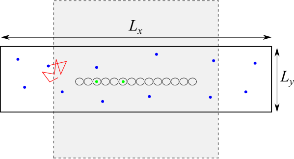
Figure 10: The reservoir is a rectangular surface. The particles in the reservoir (blue dots) are diffusing with a diffusion coefficient $D$, without interactions (a typical trajectory is shown in red). The sites of the TASEP-LK filament are modeled by $L$ disks (reaction surfaces) of diameter $a$. Particles can attach (green dots) or detach from these disks. In order to check the effect of the cross-section $L_{y}$, while keeping the size of the reservoir constant, we change $L_{x}$ and $L_{y}$ such that the volume of the reservoir $L_{x}\times L_{y}$ remains constant. This is illustrated with the gray rectangle which has a larger cross-section than the “white“ rectangle.

For simplicity, the reservoir is two-dimensional with a rectangular shape. The lengths of the edges of the rectangle are defined by $L_{x}$ and $L_{y}$ (see figure 10). The filament has a length $L_{f}$ corresponding to $L$ disks with a reaction surface of diameter $a\approx L_{f}/L$. Since the dimensions of the filament are constant during our simulations, we set the length unit $a$ of the system equal to the diameter of a disk: $a=10^{-8}m$ corresponds to the typical order of magnitude of a step done by motor proteins of the kinesin family [2]. In the simulations shown in figure 8, we choose $N=10^{3}$ particles and $L=10^{3}$ sites so that $m=1$. The reservoir has a constant surface $L_{x}\,L_{y}=50\mu m^{2}$, and so the concentration is kept constant ($c=3.32\cdot 10^{-11}mol\,m^{-2}$ for all curves in figure 8, with a length of the filament of $L_{f}=10\mu m$ and $\Omega^{\infty}_{\rm A}=1$). The other parameters $\beta/p$ and $\Omega_{\rm D}$ determine the phase of the system and vary from graph to graph.

The TASEP-LK filament is thus modeled as a sequence of disks playing the role of a reaction volume: if the site in not occupied, then a diffusive particle in the reaction volume can attach to this site at a constant rate $k$. It implies that the rate of attaching to the site $i$ is $\omega_{\rm A}(i)=k\,n(i)=\tilde{\omega}_{\rm A}c_{u}(i)$ where $n(i)$ and $c_{u}(i)$ are respectively the number of particles and the concentration of the reaction volume associated to the site $i$. Thus we have $\tilde{\omega}_{\rm A}=k\,v_{R}$ where $v_{R}$ is the volume of reaction (here the disk area). The other update rules on the filament are unchanged: particles can perform a discrete jump to the right with a rate $p$, which sets the timescale of the system; if a particle detaches at a rate $\omega_{\rm D}$ or $\beta$, then it performs diffusion in the reservoir. We fix $p=50s^{-1}$ to the order fo magnitude of measured rates for kinesins  [42]. The outcomes of simulations, figure 8, show the effect of changing the reservoir size, namely by increasing $L_{y}$. At the same time, we decrease $L_{x}$ such that the area of the reservoir and hence the other parameters remain constant, like the total concentration $c=N/(L_{x}L_{y})$ (and so $\rho^{\infty}_{\ell}$) and the parameter $m=N/L$. In that way, the system remains at the same point of the phase diagram, as we can see by considering e.g. figure 5.

The particles in the reservoir evolve according to a Brownian dynamics defined by equations (2-4) in subsection 2.3. We introduce now the finite difference $\Delta t$ instead of the derivatives in the equation of motion. The $\delta(t-t^{\prime})$ in the amplitudes of the white noise is replaced by $1/\Delta t$ where $\Delta t=t-t^{\prime}$ :

$$\frac{\vec{r}(t+\Delta t)-\vec{r}(t)}{\Delta t} = \vec{\xi}(t)\,,$$

$$r_{a}(t+\Delta t) = r_{a}(t)+\sqrt{2D\Delta t}\eta_{a}\,,$$

where $\eta_{a}$ is a random number generated with a gaussian distribution with unit variance.

After one update of the filament, the diffusion equation for the diffusing particles in the reservoir are integrated during the time of evolution of the filament given by the time interval $\tau=S_{R}^{-1}\ln(1/r)$ [44, 45], where $S_{R}$ is the sum of all the possible rates and $r$ is a random number uniformly distributed in $(0,1]$. If the position of a particle is updated outside the box, the move is rejected. To reduce these boundary effects, we split this global interval of integration in small enough time intervals.

References

References

- [1] B. Alberts, A. Johnson, J. Lewis, M. Raff, K. Roberts, and P. Walter, Molecular biology of the cell. Garland science, Taylor & Francis Group, 5 ed., 2008.
- [2] J. Howard, Mechanics of Motor Proteins and the Cytoskeleton. Sinauer Associates, 2001.
- [3] M. Schliwa, Molecular Motors. Weinheim: Wiley-VCH, 2003.
- [4] M. Schliwa and G. Woehlke, “Molecular motors,” Nature, vol. 422, pp. 759–765, Apr. 2003.
- [5] J. L. Rosenbaum and G. B. Witman, “Intraflagellar transport,” Nat Rev Mol Cell Biol., vol. 3, pp. 813–25, 2002.
- [6] J. M. Scholey, “Intraflagellar transport,” Annu. Rev. Cell Dev. Biol., vol. 19, pp. 423– 43, 2003.
- [7] P. W. Baas, C. V. Nadar, and K. A. Myers, “Axonal transport of microtubules: the long and short of it,” Traffic, vol. 7, pp. 490–8, 2006.
- [8] P. J. Hollenbeck and W. M. Saxton, “The axonal transport of mitochondria,” J Cell Sci., vol. 118, pp. 5411–9, 2005.
- [9] M. Setou, T. Hayasaka, and I. Yao, “Axonal transport versus dendritic transport,” J Neurobiol., vol. 58, pp. 201–6, 2004.
- [10] P. L. Leopold and K. K. Pfister, “Viral strategies for intracellular trafficking: Motors and microtubules,” Traffic, vol. 7, pp. 516–23, 2006.
- [11] V. Muresan and Z. Muresan, “Unconventional functions of microtubule motors,” Archives of Biochemistry and Biophysics, vol. 520, pp. 17–29, Apr. 2012.
- [12] V. Varga, J. Helenius, K. Tanaka, A. A. Hyman, T. U. Tanaka, and J. Howard, “Yeast kinesin-8 depolymerizes microtubules in a length-dependent manner,” Nature Cell Biology, vol. 8, pp. 957–962, 2006.
- [13] V. Varga, C. Leduc, V. Bormuth, S. Diez, and J. Howard, “Kinesin-8 motors act cooperatively to mediate length-dependent microtubule depolymerization,” Cell., vol. 138, pp. 1174–1183, 2009.
- [14] C. Leduc, K. Padberg-Gehle, V. Varga, D. Helbing, S. Diez, and J. Howard, “Molecular crowding creates traffic jams of kinesin motors on microtubules,” PNAS, vol. 109, no. 16, pp. 6100–6105, 2012.
- [15] A. Parmeggiani, T. Franosch, and E. Frey, “Phase coexistence in driven one-dimensional transport,” Phys. Rev. Lett., vol. 90, p. 086601, 2003.
- [16] A. Parmeggiani, T. Franosch, and E. Frey, “The totally asymmetric simple exclusion process with langmuir kinetics,” Phys. Rev. E, vol. 70, p. 046101, 2004.
- [17] R. Lipowsky, S. Klumpp, and T. M. Nieuwenhuizen, “Random walks of cytoskeletal motors in open and closed compartments,” Phys. Rev. Lett., vol. 87, p. 108101, 2001.
- [18] S. Klumpp and R. Lipowsky, “Traffic of molecular motors through tube-like compartments.,” J. Stat. Phys., vol. 113, pp. 233–268, 2003.
- [19] R. Lipowsky and S. Klumpp, “Life is motion: multiscale motility of molecular motors,” Physica A: Statistical Mechanics and its Applications, vol. 352, pp. 53–112, 2005.
- [20] M. J. I. Müller, S. Klumpp, and R. Lipowsky, “Molecular motor traffic in a half open tube,” J. Phys.: Condens. Matter, vol. 17, pp. S3839–S3850, 2005.
- [21] A. Parmeggiani, “Non-equilibrium collective transport on molecular highways,” in Traffic and Granular Flow ’07 (C. Appert-Rolland, F. Chevoir, P. Gondret, S. Lassarre, J.-P. Lebacque, and M. Schreckenberg, eds.), pp. 667–677, Springer Berlin Heidelberg, Jan. 2009.
- [22] K. Tsekouras and A. B. Kolomeisky, “Parallel coupling of symmetric and asymmetric exclusion processes,” J. Phys. A: Math. Theor., vol. 41, p. 465001, 2008.
- [23] D. A. Adams, B. Schmittmann, and R. K. P. Zia, “Far-from-equilibrium transport with constrained resources,” J Stat Mech, p. P06009, 2008.
- [24] L. J. Cook and R. K. P. Zia, “Feedback and fluctuations in a totally asymmetric simple exclusion process with finite resources,” J Stat Mech, p. P02012, 2009.
- [25] P. Greulich, L. Ciandrini, R. J. Allen, and M. C. Romano, “A mixed population of competing taseps with a shared reservoir of particles,” Phys. Rev. E, vol. 85, p. 011142, 2012.
- [26] A. Seitz and S. Thomas, “Processive movement of single kinesins on crowded microtubules visualized using quantum dots,” The EMBO Journal, vol. 25, p. 267, Jan 2006.
- [27] T. L. Blasius, N. Reed, B. M. Slepchenko, and K. J. Verhey, “Recycling of kinesin-1 motors by diffusion after transport,” PLoS ONE, vol. 8, p. e76081, 09 2013.
- [28] M. R. Evans, R. Juhász, and L. Santen, “Shock formation in an exclusion process with creation and annihilation,” Physical Review E, vol. 68, p. 026117, Aug. 2003.
- [29] T. Chou, K. Mallick, and R. K. P. Zia, “Non-equilibrium statistical mechanics: From a paradigmatic model to biological transport,” Reports on Progress in Physics, vol. 74, p. 116601, 2011.
- [30] P. C. Bressloff and J. M. Newby, “Stochastic models of intracellular transport,” Rev. Mod. Phys., vol. 85, p. 135, 2013.
- [31] D. Chowdhury, “Stochastic mechano-chemical kinetics of molecular motors: A multidisciplinary enterprise from a physicist’s perspective,” Physics Reports, 2013.
- [32] I. Langmuir, “The adsorption of gases on plane surfaces of glass, mica and platinum,” J. Am. Chem. Soc., vol. 40, pp. 1361–1403, 1918.
- [33] V. Popkov, A. Rákos, R. D. Willmann, A. B. Kolomeisky, and G. M. Schütz, “Localization of shocks in driven diffusive systems without particle number conservation,” Phys. Rev. E, vol. 67, p. 066117, Jun 2003.
- [34] J. Krug, “Boundary-induced phase transitions in driven diffusive systems,” Phys. Rev. Lett., vol. 67, pp. 1882–1885, Sep 1991.
- [35] G. Schutz and E. Domany, “Phase transitions in an exactly soluble one-dimensional exclusion process,” Journal of Statistical Physics, vol. 72, no. 1-2, pp. 277–296, 1993.
- [36] G. A. Klein, K. Kruse, G. Cuniberti, and F. Jülicher, “Filament depolymerization by motor molecules,” Phys. Rev. Lett., vol. 94, p. 108102, Mar 2005.
- [37] D. Johann, C. Erlenkämper, and K. Kruse, “Length regulation of active biopolymers by molecular motors,” Physical Review Letters, vol. 108, p. 258103, 2012.
- [38] A. Melbinger, L. Reese, and E. Frey, “Microtubule length regulation by molecular motors,” Physical Review Letters, vol. 108, p. 258104, 2012.
- [39] H. Kuan and M. D. Betterton, “Biophysics of filament length regulation by molecular motors,” Phys. Biol., vol. 10, p. 036004, 2013.
- [40] I. Neri, N. Kern, and A. Parmeggiani, “Modeling cytoskeletal traffic: an interplay between passive diffusion and active transport,” Phys. Rev. Lett., vol. 110, p. 098102, 2013.
- [41] I. Neri, N. Kern, and A. Parmeggiani, “Exclusion processes on networks as models for cytoskeletal transport,” New J. Phys., vol. 15, p. 085005, 2013.
- [42] M. J. Schnitzer and S. M. Block, “Kinesin hydrolyses one ATP per 8-nm step,” Nature, vol. 388, pp. 386–390, July 1997.
- [43] R. M. Corless, G. H. Gonnet, D. E. G. Hare, D. J. Jeffrey, and D. E. Knuth, “On the lambert w function,” Adv Comput Math, vol. 5, pp. 329–359, Dec. 1996.
- [44] D. T. Gillespie, “A general method for numerically simulating the stochastic time evolution of coupled chemical reactions,” Journal of Computational Physics, vol. 22, pp. 403–434, 1976.
- [45] D. T. Gillespie, “Exact stochastic simulation of coupled chemical reactions,” The Journal of Physical Chemistry, vol. 81, pp. 2340–2361, 1977.
- [46] A. Bortz, M. Kalos, and J. Lebowitz, “A new algorithm for monte carlo simulation of ising spin systems,” Journal of Computational Physics, vol. 17, no. 1, pp. 10 – 18, 1975.