Cluster based RBF Kernel
for Support Vector Machines

Abstract

In the classical Gaussian SVM classification we use the feature space projection transforming points to normal distributions with fixed covariance matrices (identity in the standard RBF and the covariance of the whole dataset in Mahalanobis RBF). In this paper we add additional information to Gaussian SVM by considering local geometry-dependent feature space projection. We emphasize that our approach is in fact an algorithm for a construction of the new Gaussian-type kernel.

We show that better (compared to standard RBF and Mahalanobis RBF) classification results are obtained in the simple case when the space is preliminary divided by k-means into two sets and points are represented as normal distributions with a covariances calculated according to the dataset partitioning. We call the constructed method C_kRBF, where $k$ stands for the amount of clusters used in k-means. We show empirically on nine datasets from UCI repository that C₂RBF increases the stability of the grid search (measured as the probability of finding good parameters).

1 Introduction

In most classical machine learning models we exploit the global statistical properties of the data without analysis of their exact local geometry (SVM, Neural Networks). On the other hand – density based methods (Bayes, EM) – are conceptually different approaches which often lead to completely local decision criteria.

Our approach belongs to the hybrid approaches [6, 10] which typically try to combine supervised and unsupervised techniques in one, uniform model. Some of these methods are combinations of clustering and classification techniques in either direct form [5] or using the complex, hierarchical structures of alternating algorithms [11].

In this paper, we introduce the kernel building method which exploits the local data geometry using cluster-based space partition and includes it in the constructed feature space projection. We show that even the use of k-means (with $k=2$) for the partitioning part gives interesting results. Our approach can be seen as a special case of the metric learning problem which does not change the formulation of the optimization problem being solved. As a result we give a simple and efficient method which can be easily used with existing implementations of SVM.

The constructed approach not only gives better classification results then SVM but, what is of crucial importance from the practical point of view, ,,good” results are obtained with less complex tuning required as compared to the usage of RBF or Mahalanobis RBF kernels (see Figure 1 for example of grid search results on australian dataset). It is worth noting that proposing models and methods which reduce the complexity of metaparameters tuning is of crucial importance for practical applications. One the one hand, such optimziation can be too expensive (hierarchical, ensemble based classification [11], active learning scenarios [13]) and on the other researchers from other disciplines often ignore its importance [17, 4, 12].

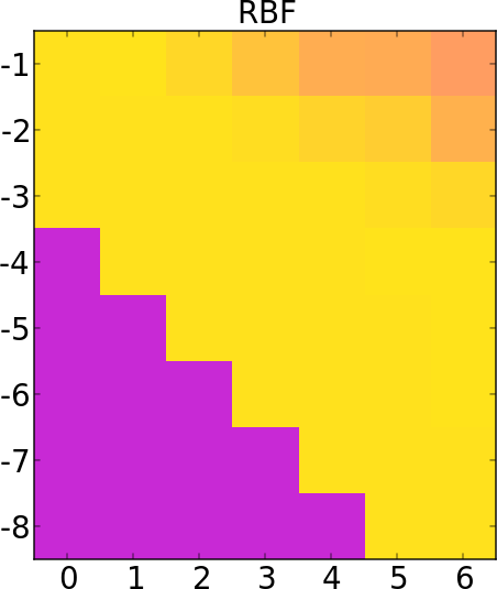
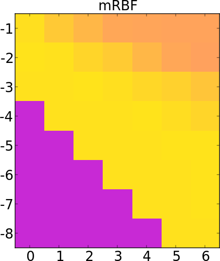
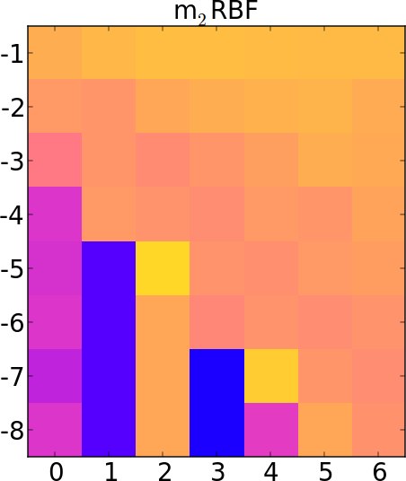
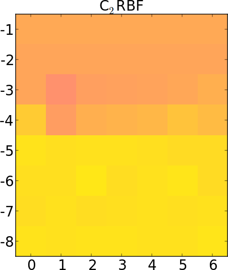
Figure 1: Accuracy scores for grid search of parameters $C$ and $\gamma$, from left: simple RBF kernel, Mahalanobis kernel, k-means + Mahalanobis kernel, our method

We also introduce an $P_{f}(\alpha)$ index (described in detail in evaluation section) able to measure how easy is to tune the model which requires some set of metaparameters and use it to evaluate our approach. It can be used both for visualization of this characteristics (similarly to how ROC curves visualize clasifier’s accuracy) and for comparision of different models (similarly to AUC ROC measure). For examples one can refer to Fig. 3 in the evaluation section.

Paper is structured as follows: first, we describe our method and prove that it leads to a valid Mercer’s kernel. Then we analyze some practical issues connected with algorithm implementation and usage and conclude with comparative empirical evaluation performed using datasets from UCI database.

2 Related work

In the recent years there is a growing interest in the fields of metric learning [18]. Among others, Mahalanobis metric learning for the RBF SVM has been proposed [9]. More computationally feasible solutions, which are similarly justified include performing preprocessing step. One of such approaches is a search for the smallest volume bounding ellipsoid [14] which is used to define the Mahalanobis kernel. Our approach is similar to this idea as it also performs a preprocessing in order to find some data characteristics but instead of optimization procedure we use cheap clustering technique.

Many researchers investigated possible fusion of k-means and SVMs – these approaches spans from using k-means to reduce the training set size [19] through reduction of support vectors count [16] to even incorporating the process of finding centroids directly into the optimization problem [5]. However, in our work k-means is used in a completely different manner, only as a selection method for the partition. Instead of reducing amount of available information (by either removing training samples or support vectors) it introduces additional kind of knowledge into the process.

Another branch of related approaches are ensembles-based models. Recently proposed HCOC [11, 7] model alternates between classification and clustering steps on many levels of tree-like structure. It also exploits some additional kind of knowledge – which classes are the most likely to be confused. Other authors also showed that clustering can be used to simply divide the problem into smaller ones solved independently by a separate classifiers [3, 8]. In C_kRBF, instead of splitting data and analyzing the output of several classifiers, we propose to include all the information gained through clustering into one, generic classifier.

3 C_kRBF kernel building algorithm

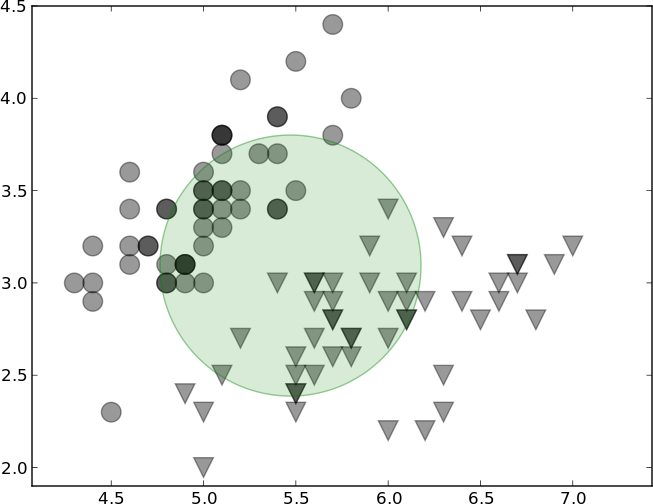
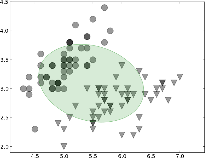
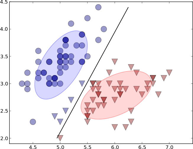
Figure 2: Comparison of $\Sigma_{x}$ matrices illustrated by ellipsoids, used in kernel projection on a subset of Iris dataset: in the leftmost picture we used RBF, on the center Mahalanobis RBF and on the right -based (the black line denotes the boundary for points being centroids of k-means solution).

The basic idea of our approach is to allow the dependence of the projection type on the local point’s neighborhood by transforming each point into some multivariate Gaussian:

$$x\to\mathcal{N}(x,\Sigma_{x}).$$

On this level of generality it leads to numerically complex problems. As we need to calculate some $\Sigma_{x}$ for every point in space. and calculate inverses of some matrices for every pair $x,y$ of points from a dataset $X$.

To make the problem more feasible we assume that we have a partition of the space into $k$ pairwise-disjoint sets

$$\mathbb{R}^{d}=W_{1}\cup\ldots\cup W_{k}\text{ where }W_{i}\cap W_{j}=\emptyset\text{ for }{i\neq j},$$

and $\Sigma_{x}$ depends only on the $x$’s belonging to an element of the partition. Consequently we fix $\Sigma_{1},\ldots,\Sigma_{k}$ and consider the feature space projection

$$x\to\mathcal{N}(x,\Sigma_{i})\text{ if }x\in W_{i},i\in\{1,\ldots,k\}.$$

Note that we still need to define $\Sigma_{i}$ for each element $W_{i}$. To avoid complex numerical optimization we simply use the empirical covariance of $X$ restricted to $W_{i}$:

$$\Sigma_{i}:=\mathrm{cov}(X\cap W_{i}).$$

The only thing left to consider is how to construct the partition $W_{i}$. To simplify this (in general infinite-dimensional) problem we assume that $W_{i}$ is given as the k-means partition of $\mathbb{R}^{d}$.

Summarizing we define the transformation $x\to\Sigma_{x}$ by the following steps:
i) choose $k>0$; ii) fix partition $W_{1},\ldots,W_{k}$ of $\mathbb{R}^{d}$; iii) define $\Sigma_{i}:=\mathrm{cov}(X\cap W_{i})$; iv) $\Sigma_{x}:=\Sigma_{i}$ if $x\in W_{i}$.

We illustrate the choice of the feature space projection on the two-dimensional projection of Iris dataset restricted to two first classes on Fig. 2.

It is worth noting that our method is somewhat similar to the ideas behind metric learning – the distance in the feature space should be better fitted to the geometry of the data. C_kRBF algorithm tries to adapt this measure to the given set of points but without incorporating it inside the optimization process. This more numerically efficient approach modifies the projection based on the neighborhood of the point in space.

There still remains the question how to choose the number $k$ and the partition $W_{i}$. In the evaluation section we show that $k=2$ is a good choice for typical datasets, and discuss some problems and benefits connected with fixing $k>2$. Clearly, in general one can select partition in an arbitrary way, including search through possible solutions of some optimization problem. In our work we focus on the simple and natural construction coming from the k-means clustering of the whole $X$.

3.1 Generalized RBF Kernel Projection

Contrary to some models we use the existing kernel space, and only modify the projection function $\phi$. We define the feature space as multivariate Gaussians, but contrary to RBF or Mahalanobis RBF we allow the variation of the Gaussians covariance over the space. Since we use the Hilbert $L^{2}(\mathbb{R}^{d})$ kernel space, we do not have to prove that the feature space projection is correct. The only thing we need is the formula for the scalar product of two points’ projections:

$$\int\mathcal{N}(m_{1},\Sigma_{1})[x]\cdot\mathcal{N}(m_{2},\Sigma_{2})[x]dx.$$

The formula for the $L^{2}$ scalar product of two Gaussians is known and can be easily deduced from the formula for the sum of two independent normal variables [15]. We provide the direct derivation here for the sake of completeness.

Lemma 3.1.

Let $m_{1},m_{2}\in\mathbb{R}^{d}$ and positive self-adjoint matrices $S_{1},S_{2}$ be given. We put

$$m =(S_{1}+S_{2})^{-1}(S_{1}m_{1}+S_{2}m_{2}),$$

$$S =S_{1}+S_{2},$$

$$W =(S_{1}^{-1}+S_{2}^{-1})^{-1}.$$

Then

$$(x-m_{1})^{T}S_{1}(x-m_{1})+(x-m_{2})^{T}S_{2}(x-m_{2})$$ (3.1)

$$= (x-m)^{T}S(x-m)+(m_{1}-m_{2})^{T}W(m_{1}-m_{2}).$$

Proof.

One can easily see that the main difficulty lies in proving that the parts ,,without” $x$ on left and right-hand sides of (3.1) coincide. Now the left hand side of (3.1) can be rewritten in the following form:

$$\begin{array}[]{l}-m^{T}Sm+m_{1}^{T}S_{1}m_{1}+m_{2}^{T}S_{2}m_{2}\\[4.30554pt] =-(m_{1}^{T}S_{1}+m_{2}^{T}S_{2})(S_{1}+S_{2})^{-1}(S_{1}m_{1}+S_{2}m_{2})\\ \phantom{=}+m_{1}^{T}S_{1}(S_{1}+S_{2})^{-1}(S_{1}m_{1}+S_{2}m_{1})\\ \phantom{=}+m_{2}^{T}S_{2}(S_{1}+S_{2})^{-1}(S_{1}m_{2}+S_{2}m_{2})\\[4.30554pt] =m_{1}^{\prime}S_{1}(S_{1}+S_{2})^{-1}S_{2}(m_{1}-m_{2})\\ \phantom{=}-m_{2}^{\prime}S_{2}(S_{1}+S_{2})^{-1}S_{1}(m_{1}-m_{2}).\end{array}$$ (3.2)

Clearly

$$\begin{array}[]{l}W=(S_{1}^{-1}+S_{2}^{-1})^{-1}=S_{1}[(S_{1}^{-1}+S_{2}^{-1})S_{1}]^{-1}=\\[2.15277pt] =S_{1}(I+S_{2}^{-1}S_{1})^{-1}=S_{1}(S_{2}^{-1}S_{2}+S_{2}^{-1}S_{1})^{-1}\\[2.15277pt] =S_{1}(S_{2}+S_{1})^{-1}S_{2}.\end{array}$$

Analogously $W=S_{2}(S_{1}+S_{2})^{-1}S_{1}$, which means that (3.2) reduces to $(m_{1}-m_{2})^{T}W(m_{1}-m_{2})$. ∎

We recall that for $m\in\mathbb{R}^{d}$ and positive self-adjoint matrix $\Sigma$ by $\mathcal{N}(m,\Sigma)$ we denote the normal density with mean $m$ and covariance matrix $\Sigma$, that is

$$\mathcal{N}(m,\Sigma)[x]:=\mbox{$\frac{1}{\sqrt{(2\pi)^{d}\det\Sigma}}$}\exp(-\tfrac{1}{2}\|x-m\|_{\Sigma}^{2}),$$

where $\|v\|^{2}_{\Sigma}$ denotes the square of Mahalanobis norm of $v$ given by $\|v\|^{2}_{\Sigma}=v^{T}\Sigma^{-1}v\mbox{ for }v\in\mathbb{R}^{d}$.

Proposition 3.1.

Let $m_{1},m_{2}\in\mathbb{R}^{d}$ and let $\Sigma_{1},\Sigma_{2}$ be positive self-adjoint matrices on $\mathbb{R}^{d}$. We have

$$\int\mathcal{N}(m_{1},\Sigma_{1})[x]\cdot\mathcal{N}(m_{2},\Sigma_{2})[x]dx=\mbox{$\frac{1}{\sqrt{(2\pi)^{d}\det(\Sigma_{1}+\Sigma_{2})}}$}\exp(-\tfrac{1}{2}\|m_{1}-m_{2}\|^{2}_{\Sigma_{1}+\Sigma_{2}}).$$

Proof.

We put $S_{i}=\Sigma_{i}^{-1}$ and define $m$ as in the previous lemma. By (3.1) we have

$$\begin{array}[]{c}\exp(-\tfrac{1}{2}\|x-m_{1}\|^{2}_{\Sigma_{1}})\cdot\exp(-\tfrac{1}{2}\|x-m_{2}\|^{2}_{\Sigma_{2}})\\[4.30554pt] =\exp(-\tfrac{1}{2}\|x-m\|^{2}_{(\Sigma_{1}^{-1}+\Sigma_{2}^{-1})^{-1}})\cdot\exp(-\tfrac{1}{2}\|m_{1}-m_{2}\|^{2}_{\Sigma_{1}+\Sigma_{2}}),\end{array}$$

which implies that

$$(2\pi)^{d}\sqrt{\det\Sigma_{1}\det\Sigma_{2}}\int\mathcal{N}(m_{1},\Sigma_{1})[x]\cdot\mathcal{N}(m_{2},\Sigma_{2})[x]dx$$

$$=\int\exp(-\tfrac{1}{2}\|x-m_{1}\|^{2}_{\Sigma_{1}})\cdot\exp(-\tfrac{1}{2}\|x-m_{2}\|^{2}_{\Sigma_{2}})dx$$

$$=\exp(-\tfrac{1}{2}\|m_{1}-m_{2}\|^{2}_{\Sigma_{1}+\Sigma_{2}})\int\exp(-\tfrac{1}{2}\|x-m\|^{2}_{(\Sigma_{1}^{-1}+\Sigma_{2}^{-1})^{-1}})dx.$$

Since

$$\int\mathcal{N}(m,(\Sigma_{1}^{-1}+\Sigma_{2}^{-1})^{-1})[x]dx =(2\pi)^{d/2}\sqrt{\det((\Sigma_{1}^{-1}+\Sigma_{2}^{-1})^{-1})}$$

$$=\frac{(2\pi)^{d}\sqrt{\det\Sigma_{1}\det\Sigma_{2}}}{(2\pi)^{d/2}\sqrt{\det(\Sigma_{1}+\Sigma_{2})}}$$

we obtain the assertion of the proposition. ∎

Theorem 3.1.

Consider a function $x\to\Sigma_{x}$ and put

$$\hat{K}_{\gamma}(x,y)=\mbox{$\frac{1}{\sqrt{(\tfrac{\pi}{\gamma})^{d}\det(\Sigma_{x}+\Sigma_{y})}}$}\exp(-\gamma\|x-y\|^{2}_{\Sigma_{x}+\Sigma_{y}}).$$

Then $\hat{K}_{\gamma}$ is a valid kernel in the Mercer’s sense for each $\gamma>0$.

Proof.

It is a direct consequence of the fact that $\hat{K}_{\gamma}$ is a scalar product in the feature space $\phi(X)\subset L^{2}(\mathbb{R}^{d})$ for feature projection defined by

$$\phi(x)=\mathcal{N}(x,(2\gamma)^{-1}\Sigma_{x}).$$

∎

This concept generalizes two mentioned RBF kernels in a natural way.

Observation 3.1.

For constant function $\Sigma_{x}=I$ our approach reduces to the classical RBF and for $\Sigma_{x}=\mathrm{cov}(X)$ (or for $k=1$ and the trivial -based calculation) to the Mahalanobis RBF (up to the scaling factor).

In practical usage, some of the $\Sigma_{x}+\Sigma_{y}$ may be not invertible, and as a consequence we cannot compute $\|x-y\|^{2}_{\Sigma_{x}+\Sigma_{y}}$. To deal with this case we ca use the typical regularization approach.

Observation 3.2.

If for some $x$ the matrix $\Sigma_{x}$ is not invertible it is sufficient to replace $\Sigma_{x}$ with $(1~{}-~{}\varepsilon)\Sigma_{x}+\varepsilon A$ for any fixed $\varepsilon\in(0,1)$ and positive matrix $A$ (then $\Sigma_{x}$ becomes positive, and consequently invertible).

In practice as $A$ we use the covariance of the whole dataset $X$, since we want to retain the geometry of the data. We also select $\varepsilon$ as small as it is reasonably possible in order to preserve our method characteristics instead of mimicking the Mahalanobis RBF approach.

One more interesting border case of our kernel is restriction on the classes of $\Sigma_{x}$ used, which leads to the computational complexity reduction.

Observation 3.3.

We can restrict the set of possible $\Sigma_{x}$ to some subset of positive self-adjoint matrices in order to obtain simpler (more efficient) kernel. By restricting to the radial Gaussians we have $\Sigma_{x}~{}=~{}\sigma_{x}^{2}I$ and consequently kernel formula for fixed $\gamma$ simplifies to

$$\mbox{$\frac{1}{\sqrt{(\tfrac{\pi}{\gamma})^{d}(\sigma_{x}^{2}+\sigma_{y}^{2})}}$}\exp(-\tfrac{\gamma}{\sigma_{x}^{2}+\sigma_{y}^{2}}\left\|x-y\right\|^{2})\propto\mbox{$\frac{1}{\sqrt{(\sigma_{x}^{2}+\sigma_{y}^{2})}}$}\exp(-\tfrac{\gamma}{\sigma_{x}^{2}+\sigma_{y}^{2}}\left\|x-y\right\|^{2}),$$

which has a computational complexity of standard RBF kernel even though each point can have its own local variance.

4 Practical considerations

For fixed $\gamma$ we may drop the constant factors from the definition of the kernel in Theorem 3.1 which leads to a more numerically efficient formula:

$$K_{\gamma}(x,y)=\mbox{$\frac{1}{\sqrt{\det(\Sigma_{x}+\Sigma_{y})}}$}\exp(-\gamma\left\|x-y\right\|^{2}_{\Sigma_{x}+\Sigma_{y}}),$$

which is implemented in Algorithm 1. As it has been already shown in Observation 3.2, in case the sum of covariances is not invertible, we can simply substitute those matrices with convex combination with the covariance of the whole set (if it is invertible, or with identity matrix otherwise) with some small $\varepsilon$.

Algorithm 1 C_kRBF kernel building

  Input: data $X$, kernel parameter $\gamma$,

  

  $X_{1},\ldots,X_{k}\leftarrow$ cluster($X$)

  $\Sigma_{i}\leftarrow\mathrm{cov}(X_{i})$ for $i\in\{1,\ldots,k\}$

  for $i\in\{1,\ldots,k\}$ do

     if $\det(\Sigma_{i})\leq 0$ then

        $\Sigma_{i}\leftarrow(1-\varepsilon)\Sigma_{i}+\varepsilon\mathrm{cov}(X)$ for small $\varepsilon\in(0,1)$

     end if

  end for

  $n_{i,j}\leftarrow\sqrt{1/\!\det(\Sigma_{i}+\Sigma_{j})}$ for $i,j\in\{1,\ldots,k\}$

  $S_{i,j}\leftarrow(\Sigma_{i}+\Sigma_{j})^{-1}$ for $i,j\in\{1,\ldots,k\}$

  $\mathrm{i}(x):=i$ where $x\in X_{i}$

  $K_{\gamma}(x,y):=n_{\mathrm{i}(x),\mathrm{i}(y)}\exp(-\gamma(x^{T}S_{\mathrm{i}(x),\mathrm{i}(y)}y))$

  return $K_{\gamma}$

Complexity of our kernel building algorithm depends on the complexity of k-means and the matrix operations (determinant, inversion) applied to the sums of local covariance matrices. In the naive implementation matrix inversion’s complexity is $O(d^{2.81})$, where $d$ is the problem’s dimensionality, so the whole process adds $O(k^{2}d^{2.81})$ complexity term to the preprocessing. As we are assuming that $d$ is relatively small (so there is a need of using RBF like kernel), this cost is negligible as this process is needed only once per given data and parameter $\gamma$. It is worth noting that for fixed $k$ the complexity of this step is asymptotically equal to the computation of Mahalanobis RBF kernel. Moreover, C_kRBF does not complicate (or deconvexify) the optimization process itself, which is the case in Mahalanobis metric learning SVM and other modifications using the additional optimization routines.

In order to avoid repeated recalculation of the determinants and inversions during cross-validation procedure we can exploit the fact that the only element that is dependent on the choice of $\gamma$ is the exponent value. After easy calculations we arrive at the kernel value conversion formula

$$K_{\hat{\gamma}}(x,y)=n_{\mathrm{i}(x),\mathrm{i}(y)}\exp(\ln(K_{\gamma}(x,y)/n_{\mathrm{i}(x),\mathrm{i}(y)})\tfrac{\hat{\gamma}}{\gamma}).$$

As the kernel building part of C_kRBF does not use labels of samples, we can build upon all the available data, including unlabeled samples as well as data from the testing set. Consequently we do not have to run it with each fold during cross-validation separately, but rather cluster the whole data and then train separate SVMs on the data subsets. This feature can be especially exploited when applied in active learning setting [13] where we have large amount of unlabeled examples.

5 Evaluation

Evaluation was performed using nine datasets from UCI repository [2], briefly summarized in Table 1. All points were linearly scaled to the $[0,1]$ interval for fair comparision with regular RBF. As one can see, almost all considered datasets show significant differences in internal geometry between clusters detected by k-means algorithm (sixth column). Only crashes data seems to be quite homogeneous.

dataset	d	n${}_{{}_{-}}$	n${}_{{}_{+}}$	$\frac{\left\|\Sigma_{1}-I\right\|}{\left\|\Sigma_{1}\right\|+\left\|I\right\|}$	$\frac{\left\|\Sigma_{2}-I\right\|}{\left\|\Sigma_{2}\right\|+\left\|I\right\|}$	$\frac{\left\|\Sigma_{2}-\Sigma_{1}\right\|}{\left\|\Sigma_{2}\right\|+\left\|\Sigma_{1}\right\|}$	$\frac{\left\|(\Sigma_{2}+\Sigma_{1})-\Sigma\right\|}{\left\|\Sigma_{2}+\Sigma_{1}\right\|+\left\|\Sigma\right\|}$
australian	14	329	361	0.574	0.549	0.151	0.363
bank	4	462	910	0.890	0.828	0.466	0.189
breast cancer	10	453	230	0.890	0.514	0.760	0.459
crashes	20	270	270	0.992	0.992	0.003	0.333
diabetes	8	515	253	0.854	0.824	0.295	0.328
fourclass	2	404	458	0.701	0.664	0.116	0.319
heart	13	129	141	0.469	0.507	0.327	0.344
liver-disorders	6	293	52	0.909	0.741	0.636	0.458
splice	60	592	408	0.331	0.361	0.265	0.328

Table 1: Characteristics of used datasets. $\Sigma_{1}$ and $\Sigma_{2}$ denotes the covariances of first and second cluster found by k-means (with $k=2$).

Experiments were performed using code written in Python with use of scikit-learn library. K-means algorithm was seeded with K-means++ [1] 10 times and clustering yielding the smallest energy was selected. All data (including test cases) was used during the clustering step (as unlabeled examples). All experiments were performed in 10-fold cross-validation mode.

We start our evaluation with reporting the best accuracy obtained by all tested models. Table 2 shows that proposed method achieves similar results to the RBF kernel and Mahalanobis RBF. In some cases C_kRBF behaves significantly better (australian, diabetes, breast-cancer) and for some worse than referencing kernels (crashes, heart, liver-disorders). These results are the consequence of many aspects – including the choice of the simplest clustering algorithm, naive empirical covariance estimation. They show, however, that in terms of achieved overall accuracy using C_kRBF leads to comparable results to RBF/mRBF based classification. To show, that our approach is fundamentally different from applying k-means as a data partitioning scheme, and training separate mRBF based models in each cluster, we also report results of such model (dentoed as m_kRBF, meaning that it first runs k-means and in each cluster trains separate cluter’s covariance based SVM).

dataset	RBF	mRBF	C2RBF	C3RBF	C4RBF	m2RBF	m3RBF	m4RBF
australian	0.862	0.856	0.872	0.875	0.859	0.838	0.801	0.797
bank	1.000	1.000	1.000	1.000	1.000	1.000	1.000	1.000
breast-cancer	0.972	0.971	0.975	0.972	0.972	0.955	0.953	0.932
crashes	0.952	0.948	0.939	0.943	0.930	0.939	0.944	0.931
diabetes	0.755	0.760	0.772	0.768	0.758	0.758	0.764	0.743
fourclass	0.996	0.996	0.996	0.996	0.996	0.996	0.996	0.996
heart	0.844	0.844	0.826	0.819	0.789	0.778	0.789	0.789
liver-disorders	0.731	0.734	0.728	0.722	0.720	0.734	0.722	0.733
splice	0.893	0.868	0.893	0.888	0.871	0.892	0.883	0.874

Table 2: Comparision of accuracy obtained by different kernels. For C_kRBF k-means is used as the clustering technique

We investigated how different clustering techniques behave in such task. We performed experiments for Gaussian Mixture Model (GMM) and Dirichlet Process Gaussian Mixture Model (DPGMM) with number of clusters varying from $2$ to $4$. Table 3 shows differences between accuracy obtained for k-means based method and Gaussian Mixture Models. One can make at least two important observations here. First, k-means performs surprisingly well as compared to more advanced clustering methods. Second, for some datasets (like liver-disorders) GMM based solution brings considerable increase in classification quality (which outperforms also RBF and mRBF, refer to Table 2). This may lead to the conclusion, that different types of clustering methods can exploit various types of knowledge. The choice of a good clustering technique requires an additonal analysis of data, internal cross-validation etc. so in further parts of our investigations we focus only on k-means based approach to show its wide applicability. However, reader should bear in mind, that different methods are possible.

dataset	C2RBF	GMM2	GMM3	GMM4	DPGMM2	DPGMM3	DPGMM4
australian	0.872	0.872	0.768	0.852	0.868	0.868	0.868
bank	1.000	1.000	1.000	1.000	1.000	1.000	1.000
breast-cancer	0.975	0.971	0.972	0.965	0.971	0.971	0.971
crashes	0.939	0.951	0.943	0.933	0.946	0.946	0.946
diabetes	0.772	0.744	0.755	0.736	0.767	0.767	0.767
fourclass	0.996	0.996	0.996	0.996	0.996	0.996	0.996
heart	0.826	0.815	0.807	0.815	0.844	0.844	0.844
liver-disorders	0.728	0.739	0.737	0.748	0.722	0.722	0.722
splice	0.893	0.877	0.887	0.864	0.866	0.866	0.866

Table 3: Comparision of accuracy of proposed method with various clustering methods. K-means is used for C₂RBF

The most interesting effect of using the proposed method is easier metaparameters selection. In practice, many applied researchers (for example in cheminformatics [17, 4, 12]) neglect the metaparameters optimization and use its default values. In most of existing SVM libraries (including libSVM, WEKA), the default value of the $C$ metaparameter is $1$. Table 4 shows accuracy obtained by considered models once we narrow down to the optimization of only $\gamma$. C₂RBF obtaines significantly better results than both RBF and mRBF in most cases. It achieves worse performance than RBF kernel only in two tests, where also mRBF behaved worse, which simply shows, that in these datasets, covariance based geometry is not a good kernel building base.

dataset	RBF	mRBF	C2RBF	C3RBF	C4RBF	m2RBF	m3RBF	m4RBF
australian	0.855	0.857	0.862	0.862	0.859	0.762	0.801	0.791
bank	0.978	1.000	1.000	1.000	1.000	0.999	1.000	1.000
breast-cancer	0.968	0.960	0.971	0.971	0.968	0.887	0.886	0.884
crashes	0.946	0.935	0.939	0.943	0.930	0.922	0.922	0.922
diabetes	0.751	0.760	0.772	0.759	0.756	0.758	0.763	0.730
fourclass	0.731	0.778	0.778	0.841	0.849	0.852	0.897	0.891
heart	0.844	0.830	0.815	0.789	0.789	0.744	0.778	0.737
liver-disorders	0.580	0.708	0.728	0.708	0.696	0.717	0.685	0.713
splice	0.833	0.840	0.893	0.888	0.871	0.883	0.868	9.842

Table 4: Comparision of accuracy obtained by different kernels when using (default) parameter value $C=1$. For C_kRBF k-means is used as the clustering technique

To further invesigate this phenomen we also performed experiments with very limited search of parameters. We fixed $C=1$ and searched through just $3$ values of $\gamma$ ($\gamma\in\{10^{i},10^{i+1},10^{i+2}\}$ for $i\in\{0,-1,-2,-3,-4,-5\}$). In Table 5 we report percentage of wins (times that C_kRBF obtained better accuracy) for each of such small tests. One can notice, that in such small metaparameters ranges, proposed method outperformed RBF and mRBF in almost all cases. Such results are of great importance in applications where we often have limited resources and many internal cross-validation based parameters selection are not possible. One such application could be the active learning scenario, or the hierarchical/ensamble based models.

	C2RBF vs		C3RBF vs		C4RBF vs
dataset	RBF	mRBF	RBF	mRBF	RBF	mRBF
australian	67%	67%	50%	50%	50%	50%
bank	100%	83%	100%	83%	100%	83%
breast-cancer	67%	100%	67%	100%	67%	100%
crashes	23%	67%	67%	100%	67%	67%
diabetes	100%	100%	83%	50%	83%	50%
fourclass	100%	83%	100%	83%	100%	100%
heart	50%	67%	50%	67%	50%	67%
liver-disorders	83%	83%	100%	83%	100%	83%
splice	83%	83%	100%	100%	100%	100%

Table 5: Percentage of 3 element wide search for $\gamma$ values with fixed $C=1$ for which given C_kRBF (based on k-means) achieved higher accuracy than corresponding kernel. Bolded values indicate values bigger than 50%

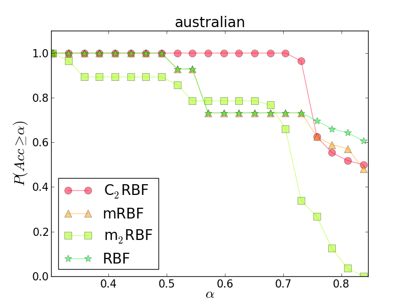
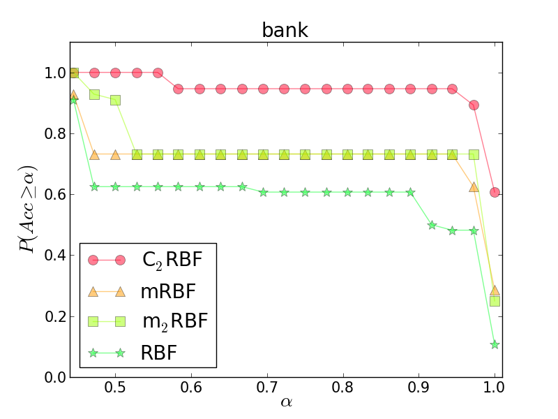
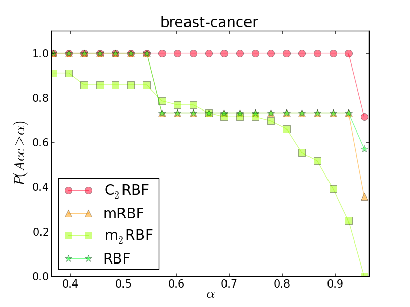
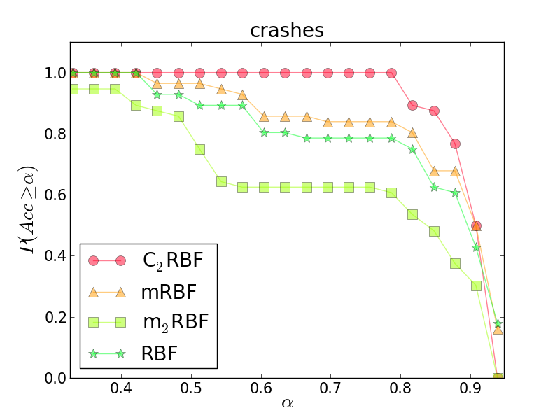
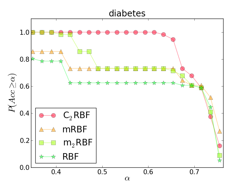
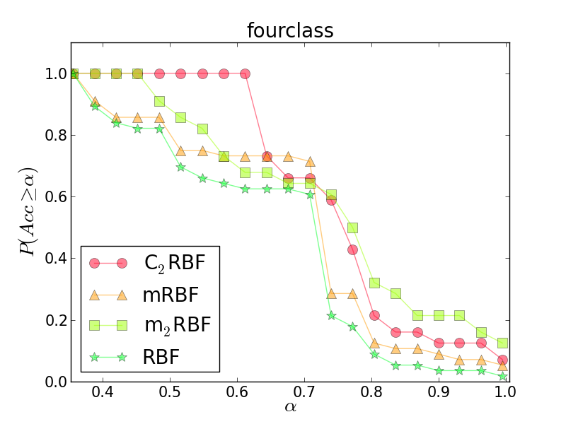
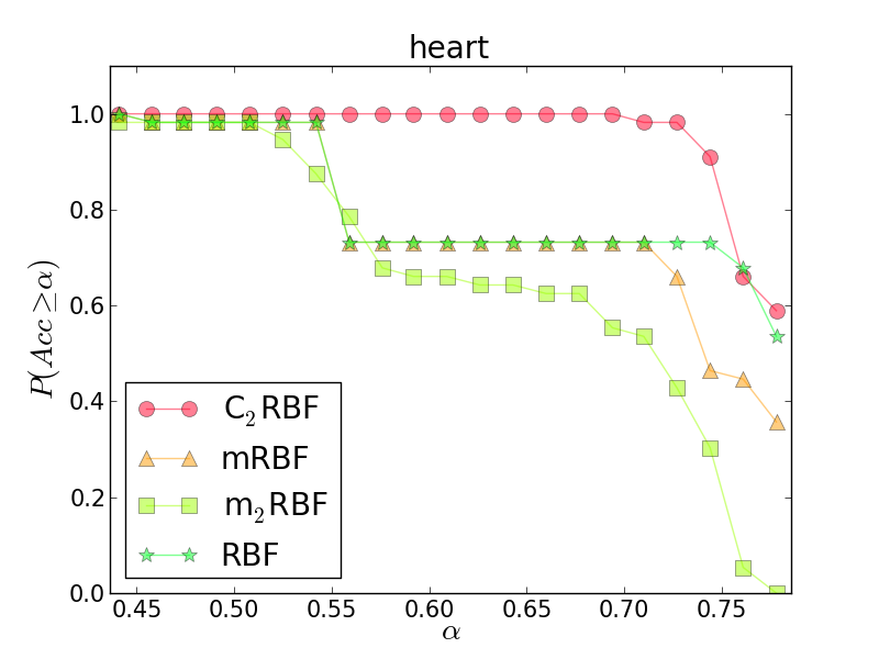
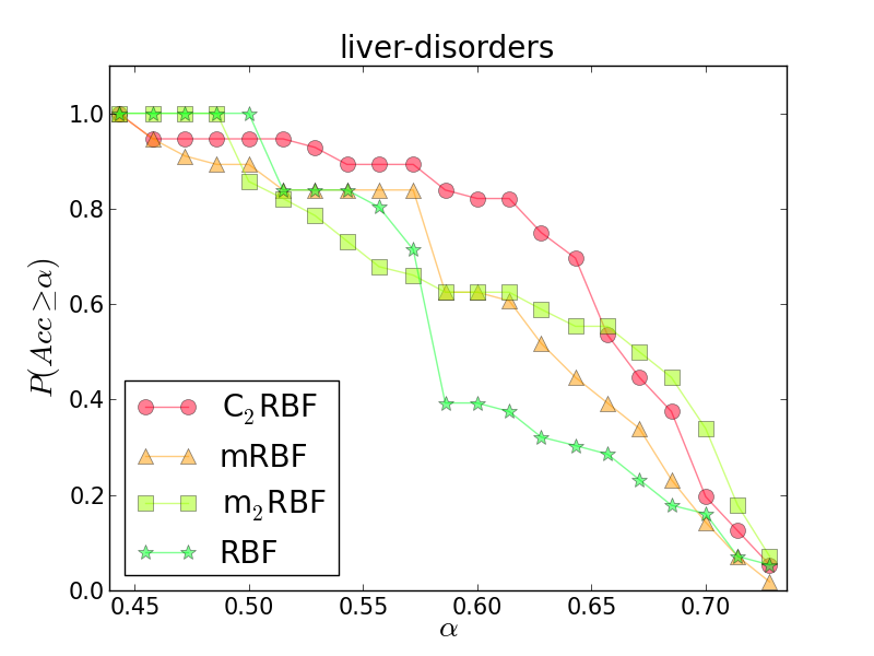
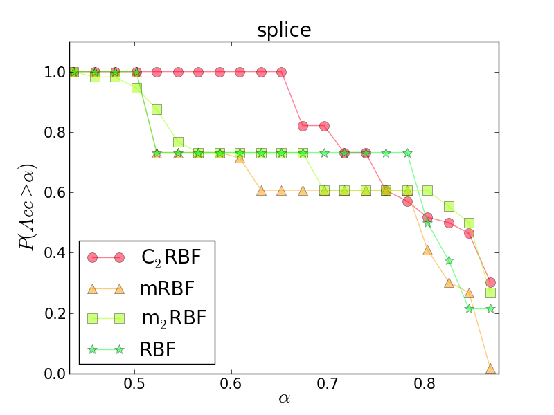
Figure 3: Visualizaion of $P_{f}(\alpha)$ for conducted experiments for C₂RBF based on k-means algorithm, regular RBF kernel and mRBF.

dataset	RBF	mRBF	C2RBF	C3RBF	C4RBF	m2RBF	m3RBF	m4RBF
australian	0.424	0.421	0.475	0.404	0.435	0.302	0.313	0.284
bank	0.328	0.400	0.526	0.530	0.531	0.414	0.413	0.408
breast-cancer	0.478	0.475	0.583	0.581	0.579	0.401	0.396	0.394
crashes	0.485	0.513	0.569	0.578	0.562	0.401	0.411	0.412
diabetes	0.253	0.288	0.361	0.344	0.347	0.302	0.313	0.284
fourclass	0.290	0.329	0.400	0.417	0.406	0.385	0.359	0.367
heart	0.331	0.320	0.387	0.382	0.375	0.285	0.269	0.272
liver-disorders	0.160	0.178	0.209	0.213	0.204	0.190	0.186	0.183
splice	0.306	0.280	0.354	0.386	0.360	0.308	0.307	0.293

Table 6: Comparision of AUC of $P_{f}(\alpha)$ obtained by different kernels. For C_kRBF k-means is used as the clustering technique

Observe that in practice, even if we perform metaparameters optimization, we never find the real optimum (in terms of tunable parameters) and therefore the increase in resolution of the grid results in finding better classification results. Thus the comparison of two SVM-based classification methods with just comparing the best result found on the grid can be misleading. We propose a measure which in our opinion is more reliable – estimation of the probability of finding results which are better than a fixed parameter value $\alpha$.

Consider the typical case in RBF SVM when our function depends on two parameters $C$ and $\gamma$. Let us fix a grid $G$ (Cartesian product of considered $C$’s and $\gamma$’s) and consider the function

$$P_{f}(\alpha):=\mathrm{prob}\{f(C,\gamma)\geq\alpha:(C,\gamma)\in G\}.$$

The above function measures the probability of finding results better then $\alpha$. As this kind of measure better exploits the model’s ability to work well with limited grid size, it directly corresponds to its applicability in training time limited scenarios. It is of great practical importance for the models which are build from many models (ensembles, hierarchical models) as well as in the active learning setting, when one has to retrain it repeatedly. We approximate this probability by the fraction of parameters pairs in the considered grid, which yield results at least $\alpha$.

$$P_{f}(\alpha)\approx\hat{P}_{f}(\alpha):=\frac{\#\{(C,\gamma)\in G:f(C,\gamma)\geq\alpha\}}{\#G}.$$

Plots of corresponding $\hat{P}_{f}$ functions in Fig. 3 illustrate that RBF and mRBF kernels are very similar in context of how hard is to find the parameters yielding good results. Also m₂RBF behaves in a very similar fashion, yielding in most cases – results between the one given by RBF and mRBF. In the same time C₂RBF offers noticeably higher probability of yielding comparable results. This observation is purely empirical and the justification of this phenomenon remains for us an open question.

Areas under the $\hat{P}_{f}$ curves (AUC) are shown in Table 6. For simplicy, we consider only curves for $\alpha$ at least as big, as the worst score achieved by all models (as $P_{f}(\alpha)$ for smaller values is constantly equal to $1$ for each model). In all conducted experiments, C₂RBF shows significant improvement over competitive approaches, confirming our claim, that C_kRBF based on k-means can be used to simplify the process of metaparameters selection.

6 Conclusions

In this paper we have presented the method of including information regarding local problem’s geometry inside the definition of the Gaussian kernel. From theoretical point of view proposed method leads to the correct kernel in the Mercer’s sense which is based on feature space projection transforming data points into various multivariate Gaussian density functions.

From practical perspective, our method’s kernel building complexity is asymptotically equivalent to the Mahalanobis RBF kernel and is similarly cheap in computation during classification. Obtained results show that our method behaves similarly to RBF and mRBF kernels. However, C_kRBF yields better results with higher probability in terms of selecting the typical SVM parameters, $C$ and $\gamma$.

We have also shown empirically that proposed approach is fundamentally different from splitting the problem into subproblems using some clustering method and building separate model for each of them. C_kRBF uses clustering in order to augment the data representation with additional knowledge instead of reducing the amount of information available. This shows the conceptual distinction of our approach from previous models.

It is also worth noting that even though we used k-means in our experiments, proposed method can be seen as more general framework, where assignment of $\Sigma_{x}$ can be the result of an arbitrary complex process. In particular, it would be interesting to further investigate space partitioning given by other supervised, linear classifiers instaed of clustering methods.

References

- [1] Arthur, D., Vassilvitskii, S.: k-means++: the advantages of careful seeding. In: Proceedings of the eighteenth annual ACM-SIAM symposium on Discrete algorithms, SODA ’07, pp. 1027–1035. Society for Industrial and Applied Mathematics (2007)
- [2] Bache, K., Lichman, M.: UCI machine learning repository (2013). URL http://archive.ics.uci.edu/ml
- [3] Baruque, B., Porras, S., Corchado, E.: Hybrid classification ensemble using topology-preserving clustering. New Generation Computing 29(3), 329–344 (2011)
- [4] Cong, Y., Yang, X.G., Lv, W., Xue, Y.: Prediction of novel and selective TNF-alpha converting enzyme (TACE) inhibitors and characterization of correlative molecular descriptors by machine learning approaches. Journal of molecular graphics & modelling 28(3), 236–44 (2009)
- [5] Gu, Q., Han, J.: Clustered support vector machines. In: Proceedings of the International Conference on Artificial Intelligence and Statistics, Journal of Machine Learning Research: W&CP, vol. 31 (2013)
- [6] Hinton, G., Osindero, S., Teh, Y.: A fast learning algorithm for deep belief nets. Neural Computation 18(7), 1527–1554 (2006)
- [7] Jackowski, K., Krawczyk, B., Woźniak, M.: Improved adaptive splitting and selection: The hybrid training method of a classifier based on a feature space partitioning. International Journal of Neural Systems (2014)
- [8] Lipka, N., Stein, B., Anderka, M.: Cluster-based one-class ensemble for classification problems in information retrieval. In: Proceedings of the 35th international ACM SIGIR conference on Research and development in information retrieval, SIGIR ’12, pp. 1041–1042. ACM (2012)
- [9] Liu, Y., Caselles, V.: Improved support vector machines with distance metric learning. In: J. Blanc-Talon, R. Kleihorst, W. Philips, D. Popescu, P. Scheunders (eds.) Advances Concepts for Intelligent Vision Systems, Lecture Notes in Computer Science, vol. 6915, pp. 82–91. Springer Berlin Heidelberg (2011)
- [10] Ma, X., Luo, P., Zhuang, F., He, Q., Shi, Z., Shen, Z.: Combining supervised and unsupervised models via unconstrained probabilistic embedding. In: Proceedings of the Twenty-Second international joint conference on Artificial Intelligence, IJCAI’11, pp. 1396–1401. AAAI Press (2011)
- [11] Podolak, I., Roman, A.: Theoretical foundations and experimental results for a hierarchical classifier with overlapping clusters. Computational Intelligence 29(2), 357–388 (2013)
- [12] Sakiyama, Y., Yuki, H., Moriya, T., Hattori, K., Suzuki, M., Shimada, K., Honma, T.: Predicting human liver microsomal stability with machine learning techniques. Journal of molecular graphics & modelling 26(6), 907–15 (2008)
- [13] Settles, B.: Active Learning, vol. 6. Morgan & Claypool Publishers (2012)
- [14] Shivaswamy, P., Jebara, T.: Ellipsoidal kernel machines. Journal of Machine Learning Research 2, 484–491 (2007)
- [15] Timm, N.: Applied multivariate Analysis. Springer Text in Statistics (2002)
- [16] Wang, J., Wu, X., Zhang, C.: Support vector machines based on k-means clustering for real-time business intelligence systems. International Journal of Bussiness Intelligence and Data Minning 1(1), 54–64 (2005)
- [17] Wang, M., Yang, X.G., Xue, Y.: Identifying hERG Potassium Channel Inhibitors by Machine Learning Methods. QSAR & Combinatorial Science 27(8), 1028–1035 (2008)
- [18] Weinberger, K., Saul, L.: Distance metric learning for large margin nearest neighbor classification. Journal of Machine Learning Research 10, 207–244 (2009)
- [19] Yao, Y., Liu, Y., Yu, Y., Xu, H., Lv, W., Li, Z., Chen, X.: K-SVM: An effective svm algorithm based on k-means clustering. Journal of Computers 8(10) (2013)