Experimental Evaluation of Multi-Round Matrix Multiplication on MapReduce

Abstract

A common approach in the design of MapReduce algorithms is to minimize the number of rounds. Indeed, there are many examples in the literature of monolithic MapReduce algorithms, which are algorithms requiring just one or two rounds. However, we claim that the design of monolithic algorithms may not be the best approach in cloud systems. Indeed, multi-round algorithms may exploit some features of cloud platforms by suitably setting the round number according to the execution context.

In this paper we carry out an experimental study of multi-round MapReduce algorithms aiming at investigating the performance of the multi-round approach. We use matrix multiplication as a case study. We first propose a scalable Hadoop library, named M₃, for matrix multiplication in the dense and sparse cases which allows to tradeoff round number with the amount of data shuffled in each round and the amount of memory required by reduce functions. Then, we present an extensive study of this library on an in-house cluster and on Amazon Web Services aiming at showing its performance and at comparing monolithic and multi-round approaches. The experiments show that, even without a low level optimization, it is possible to design multi-round algorithms with a small running time overhead.

1 Introduction

MapReduce is a computational paradigm for processing large-scale data sets in a sequence of rounds executed on conglomerates of commodity servers [6]. This paradigm, and in particular its open source implementation Hadoop [22], has emerged as a de facto standard and has been widely adopted by a number of large Web companies (e.g., Google, Yahoo!, Amazon, Microsoft) and universities (e.g., CMU, Cornell) [10]. MapReduce was initially introduced for log processing and web indexing but it has also been successfully used for other applications, including machine learning [13], data mining [2], scientific computing [20], and bioinformatics [21]. Informally, a MapReduce algorithm transforms an input multiset of key-value pairs into an output multiset of key-value pairs in a sequence of rounds. Each round consists of three steps: each input pair is individually transformed into a multiset of new pairs by a map function (map step); then the new pairs are grouped by key (shuffle step); finally, each group of pairs with the same key is processed, separately for each key, by a reduce function that produces the next new set of key-value pairs (reduce step). The MapReduce paradigm has a functional flavor, in that it merely requires that the algorithm designer specifies the computation in terms of map and reduce functions. This enables parallelism without forcing an algorithm to cater for the explicit allocation of processing resources. Nevertheless, the paradigm implicitly posits the existence of an underlying unstructured and possibly heterogeneous parallel infrastructure, where the computation is eventually run. For these reasons, the MapReduce paradigm has gained popularity in recent years in cloud services for the development of large scale computations. Indeed, MapReduce is currently offered as a service by prominent cloud providers, such as Amazon Web Services and Microsoft Azure.

As MapReduce is increasingly used for solving computational hungry problems on large datasets, it is crucial to design efficient and scalable algorithms. Many research efforts have been dedicated to capture efficiency in MapReduce algorithms (e.g.,[12, 10, 16, 2, 8]). The major source of inefficiency is the communication required for moving data from mappers to reducers in the shuffle step: since communication is a major factor determining the performance of algorithms on current computing systems, the amount of shuffled data should be minimized. Another issue that is usually taken into account for improving performance is the number of rounds of a MapReduce algorithm, since the initial setups of a round and the shuffle step are very costly operations. Thus, several MapReduce algorithms have been designed that require a very small number, usually one or two, of rounds (e.g., [2, 10]). We denote with monolithic algorithm a MapReduce algorithm requiring one or two rounds. A common approach for obtaining a monolithic algorithm is to decompose the problem into small subproblems which are executed concurrently in a single round, with each subproblem solved by a single application of the reduce function.

In this paper, we claim that the design of monolithic algorithms may not be the best approach for long running MapReduce computations in cloud systems. Although it is true that the best performance is usually reached by reducing the round number, monolithic MapReduce algorithms may not exploit some features of cloud computing. Some examples follow.

• Service market. Some cloud providers offer a market where it is possible to bid on the cost of a service and to use it only when the actual price is below the bid. For reducing computing costs of long but low-priority computations, it would be desirable to develop MapReduce algorithms that can be stopped and restarted according to the price of the service. Unfortunately, current implementations of the MapReduce paradigm do not allow to stop a computation at an arbitrary point and then restart it. However, it is possible, like in Hadoop, to restart a computation from the beginning of the round that has been interrupted, losing the work that was already executed in that round. This clearly penalizes monolithic algorithms that consist of just a few long rounds: stopping a round and waiting for a better price might not be convenient since a significant part of previous work has to be executed again. It would be then interesting to develop MapReduce algorithms featuring a larger number of short rounds in order to reduce the amount of discarded work.

• Resource requirements. Some MapReduce algorithms need strong resource requirements in order to be monolithic. For instance, the multiplication in a semiring of two dense matrices of size $\sqrt{n}\times\sqrt{n}$ in two rounds must [16] exchange approximately $n\sqrt{n/m}$ pairs during each shuffle, where $m$ denotes an upper bound to the memory that can be used by a map/reduce function. This amount of data is linear in the input size only if $m\sim n$, that is, when the multiplication can be almost solved sequentially. Similar requirements are also needed for joining relations [2] and enumerating triangles in a graph [15]. In a big-data era, the required local memory may exceed system resources and the huge amount of data in the shuffle step could arise issues related to network performance and system failure. Indeed, the network may be subject to congestion due to the large amount of data created within a small time interval, penalizing the scalability and fault tolerance of the network. It is then desirable to design algorithms that can tradeoff round number and resource requirements. We also observe that distributing a large computation among different rounds may help to checkpoint the computation and thus to restore it if the system completely fails or is heavily penalized by a fault.
  

It is then interesting to investigate multi-round algorithms where the round number can be set according to the execution context. However it is challenging to guarantee performance similar to the ones provided by monolithic algorithms. The first issue is that, by distributing the computation among different rounds, the total amount of communication in the shuffle steps should not increase with respect to the monolithic version since, as we have already mentioned, communication is the main bottleneck. Moreover, the latency required by each new round should be amortized by a sufficient amount of computation and communication performed within the round.

Our results.

In this paper we carry out an experimental study of multi-round MapReduce algorithms for matrix multiplication aiming at investigating the performance of the multi-round approach. Matrix multiplication is an important building block for many problems arising in different contexts, in particular scientific computing and graph processing [7]. Furthermore, we believe that matrix multiplication is an interesting problem for studying multi-round algorithms since its high, but still tractable, communication and computation requirements allow to significantly load the system and to assess the performance under stress. The results provided in the paper are the following:

1. We propose a scalable Hadoop library, named M₃ (Matrix Multiplication in MapReduce), for performing dense and sparse matrix multiplication in Hadoop. The library is based on the multi-round algorithms proposed in [16] which exploit a 3D decomposition of the problem. We fill the gap between the theoretical and high-level results in [16] and the actual implementation by providing a detailed description of the map and reduce functions. For the sake of completeness, M₃ also contains a MapReduce algorithm for dense matrix multiplication based on a 2D approach, which is described in Section 3.3. The algorithms exhibit a tradeoff among round number, the amount of data in the shuffle steps and the amount of memory required by each reduce function. The library is publicly available at http://www.dei.unipd.it/m3.

2. We carry out an extensive experimental evaluation of the M₃ library on an in-house cluster and on Amazon Elastic MapReduce, and show that the 3D algorithms efficiently scale with increasing input size and processor number. We compare the performance of the multi-round approach with the monolithic one by measuring the performance of our algorithms when the round number increases. The experiments show that the running times are mainly dominated by the amount of communication, while the round number has a limited impact on performance. This fact suggests that the common use (in particular in more application-oriented contexts) to only focus on round number when designing MapReduce algorithms is not a best practice for improving performance. The results also give evidence that multi-round algorithms have performance comparable with monolithic ones (assuming a similar total amount of communication) even on the Hadoop framework, which is not the most suitable MapReduce implementation for executing multi-round algorithms. Indeed, the architectural choice of Hadoop to store pairs between rounds on the distributed file system HDFS significantly penalizes the performance. We believe that other implementations (e.g., Spark [23]) may almost remove the performance gap and stimulate the adoption of multi-round algorithms.
   

We remark that the performance of our algorithms should not be compared with state-of-the-art research on parallel sparse/dense matrix multiplication in High Performance Computing (e.g., [4]). Indeed, we are interested in investigating algorithm performance in cloud systems with MapReduce. In these settings, abstraction layers add a significant burden to algorithm performance. Research on the reduction of this load is crucial (see, e.g. [23, 17]), but it is out of the scope of this paper.

Previous Work.

The MapReduce [6] paradigm has been widely studied and we refer to the book by Lin and Dyer [11] for a survey. The design of efficient MapReduce algorithms has been investigated from practical and theoretical perspectives. For instance, best practices in designing large-scale algorithms in MapReduce are proposed in [1, 12], while theoretical models for analyzing MapReduce are studied in [10, 16, 8, 2]. The majority of the algorithms requires just a few rounds, although monolithic solutions are not known for some problems (e.g., computing the diameter of a graph [5] or matrix inversion [16]). Multi-round algorithms that trade round number with resource requirements have been proposed, with a theoretical approach, in [16] for some linear algebra problems, including matrix multiplication, in [8] for sorting and searching, and in [15] for triangle enumeration. To the best of our knowledge, the only experimental analysis of multi-round algorithms has been provided in [15] for triangle enumeration and shows that the performance of a multi-round approach is equivalent to a monolithic one.

Matrix multiplication is one of the most studied problems in the literature and we refer to the book by Golub and Van Loan [7] for further insights. However, to the best of our knowledge, this problem has been scarcely studied in MapReduce: ignoring naive implementations available on the web, the only scientific works are the aforementioned [16], and [18]. The latter introduces a library, named HAMA, including MapReduce algorithms for matrix multiplication and conjugate gradient for matrices stored in HBase databases.

Comparison with previous work.

This work completes the theoretical investigations in [16] by integrating the original description with more details that allow to fill the gap between theory and practice, and by proposing an Hadoop implementation. The M₃ library includes as special case the algorithms in HAMA [18]: the iterative approach proposed in HAMA requires $\sqrt{n}$ rounds for multiplying a matrix of size $\sqrt{n}\times\sqrt{n}$ and is a special case of the algorithm based on the 2D approach described in Section 3.3 (i.e., it suffices to set $m=\sqrt{n}$ and $\rho=1$). Since the HAMA library assumes a very different input representation and our experiments show that the aforementioned 2D approach is slower than the 3D approach, we do not take into account HAMA in this paper. Moreover, it should be said that the algorithms in [18] break the functional approach of MapReduce by allowing concurrent accesses to the distributed file system within each map and reduce function, and that the experiments have been carried out on small inputs (input side $\sqrt{n}\leq$ 5000, while we run our algorithms with input side $\sqrt{n}\geq$ 16000).

Paper organization.

Section 2 introduces the matrix multiplication problem, the MapReduce framework and the experimental settings. Section 3 describes and analyzes the proposed MapReduce algorithms. Section 4 shows some additional technicalities required by the Hadoop implementation. Section 5 provides and explains the experimental results. Finally, Section 6 gives some final remarks.

2 Preliminaries

Matrix multiplication.

The focus of the paper is matrix multiplication in a general semiring, that is we are ruling out Strassen-like algorithms. For the sake of simplicity, we focus on square matrices of size $\sqrt{n}\times\sqrt{n}$. We denote with $A$ and $B$ the two input matrices and with $C=A\cdot B$ the output matrix. In the sparse case, we denote with $0\leq\delta\leq 1$ the density of non-zero entries in a given matrix of size $\sqrt{n}\times\sqrt{n}$, that is the number of non-zero entries is $\delta n$. A random Erdös-Rényi matrix of size $\sqrt{n}\times\sqrt{n}$ and parameter $0\leq\delta\leq 1$ is a matrix where each entry is non-zero with probability $\delta$ independently; the expected density is clearly $\delta$. When $\delta<<1/n^{1/4}$, the expected density of the product of two Erdös-Rényi matrices is $\delta^{2}\sqrt{n}$ [3].

MapReduce and Hadoop.

A MapReduce algorithm consists of a sequence of rounds. The input/output of a round is a multiset of key-value pairs $\langle k;v\rangle$, where $k$ and $v$ denote the key and the value respectively. The input of a round may contain the output of previous rounds but also other pairs. A round is organized in three steps:

1. Map step: each input pair is individually given in input to a map function, which returns a new multiset of pairs. The pairs returned by all applications of the map function are called intermediate pairs.

2. Shuffle step: the intermediate pairs are grouped by key.

3. Reduce step: each group of pairs associated with the same key is individually given to a reduce function, which returns a new multiset of pairs. The pairs returned by all applications of the reduce function are the output pairs of the round.
   

For simplicity we refer to a single application of the map (resp., reduce) function with mapper (resp., reducer). For a MapReduce algorithm, we denote with round number the number of rounds, with shuffle size the maximum number of intermediate pairs in each round, and with reducer size the maximum amount of memory words required by each reducer.

Hadoop[22] is the most used open source implementation of the MapReduce paradigm. A MapReduce algorithm is executed by Hadoop on $p$ processors roughly as follows. In each round, each processor is associated with a fixed number of map tasks and reduce tasks. In the map step, the runtime system evenly distributes the input pairs to the map tasks and then each map task applies the map function to each single pair. In the reduce step, all groups of same-key pairs are randomly assigned to each reduce task and then each reduce task applies the reduce function to each single group. The input/output pairs are stored in the distributed file system HDFS [19], while intermediate pairs are temporarily stored on the disk of each machine. Hadoop allows to personalize different settings of the framework, in particular it allows to specify how groups are distributed among reduce tasks by defining a partitioner. A partitioner receives as input a key $k$ and the total number $T$ of reduce tasks, and it returns a value in $[0,T)$ uniquely denoting the reduce task that will apply the reduce function to the group associated with key $k$.

We recall that there exist other efficient implementations of the MapReduce paradigm, including Spark [23], MapReduce-MPI[17], Sphere [9]. Our algorithms can be executed on these frameworks with minor programming changes.

Experimental Framework.

The in-house cluster consists of 16 nodes, each equipped with a 4-core Intel i7 processor Nehalem @ 3.07GHz, 12 GB of memory, 6 disks of 1TB and 7200 RPM in RAID0. The interconnection system is a 10 gigabit Ethernet network. The operating system is Debian/Squeeze with kernel 2.6.32. All experiments have been executed with Hadoop 2.4.0 on 16 nodes (1 master + 16 slaves; a node was both master and slave).

The experiments on Amazon Web Services have been executed on instances of type c3.8xlarge and i2.xlarge in the US East Region. The c3.8xlarge is a compute optimized instance featuring 32 virtual cores on a physical processor Intel Xeon E5-2680 @2.8GHz, 64 GB of memory, 2 solid state disks of 320 GB; instances are connected by a 10 gigabit network. The i2.xlarge is a storage optimized instance featuring 4 virtual cores on a physical processor Intel Xeon E5-2670 @2.5GHz, 32 GB of memory, 1 solid state disk of 800 GB optimized for very high random I/O performance; instances are connected by a moderate-performance network. All experiments have been run on clusters with 9 (1 master + 8 slave) instances of the same type, with a Debian/Squeeze operating system and Hadoop 2.2.0.

3 Algorithms

The M₃ library contains two MapReduce algorithms for performing matrix multiplication which are based on the 3D approach proposed in [16]. In this section, we first propose the algorithm for multiplying two square dense matrices. Then, we give the algorithm that multiplies two sparse matrices; although it applies to any sparse input, we analyze it in the case of random Erdös-Rényi matrices. The algorithms exhibit tradeoff among round number, shuffle size and reducer size, and rely on the well-know 3D decomposition of the lattice representing the $n^{3/2}$ elementary products (some of which are zeros in the sparse case) into cubes of a given size. In other words, the problem is decomposed into multiplications of smaller square matrices that are solved sequentially by the reducers. The subproblems are evenly distributed among the rounds in order to guarantee the specified tradeoff.

For the sake of comparison, we also provide in Section 3.3 an algorithm for dense matrix multiplication which is based on the 2D decomposition of the lattice: the problem is decomposed into the multiplication of smaller rectangular matrices where the longest side is $\sqrt{n}$. This approach is quite common in naive implementations of matrix multiplication in MapReduce available on the web: however, as we will see, this approach is inefficient. The algorithm exhibits a tradeoff among round number, shuffle size, and reducer size. This result does not appear in [16].

The tradeoffs in our algorithms are highlighted by expressing the round number as a function of two parameters: the replication factor $\rho$ and the subproblem size $m$. The replication factor gives an estimate of the desired volume of intermediate data in each round, while the subproblem size bounds the memory requirements of each reducer: indeed, our algorithms guarantee that the shuffle size is ${\Theta}\left(\rho\right)$ times the input size and the reducer size is ${\Theta}\left(m\right)$.

3.1 3D Algorithm for Dense Matrix Multiplication.

Map: input $\left\langle(i,\ell,j);D\right\rangle$; $D$ is $A_{i,j}$ or $B_{i,j}$ if $\ell=-1$,

        or $C^{\ell}_{i,j}$ otherwise;

      switch $D$ do

           case $D$ is $A_{i.j}$

                for $\ell$ $\leftarrow$ 0 to $\rho-1$ do

                     $h$ $\leftarrow$ $j-i-\ell$

                     emit $\left\langle(i,j,h);D\right\rangle$

                    

                    

                     case $D$ is $B_{i.j}$

                          for $\ell$ $\leftarrow$ 0 to $\rho-1$ do

                               $h$ $\leftarrow$ $i-j-\ell$

                               emit $\left\langle(h,i,j);D\right\rangle$

                              

                              

                               case $D$ is $C^{\ell}_{i.j}$

                                    if $r$ is the last round then

                                         emit $\langle(i,-1,j);D\rangle$

                                        

                                         else

                                              $h$ $\leftarrow$ $i+j+\ell+r\rho$

                                              emit $\langle(i,h,j);D\rangle$

                                             

                                             

                                             

                                             

                                             

                                              Reduce: input $\langle(i,h,j);\{A_{i,h},B_{h,j},C_{i,j}^{\ell}\}\rangle$ if $0\leq i,j<\sqrt{n/m}$ and $h=(i+j+\ell+r\rho)\mod\sqrt{n/m}$, or $\langle(i,-1,j);\{C_{i,j}^{0},\ldots C_{i,j}^{\rho-1}\}\rangle$

                                                   if $r$ is the last round then

                                                        emit $\langle(i,j);\sum_{\ell=0}^{\rho-1}C_{i,j}^{\ell}\rangle$

                                                       

                                                        else

                                                             emit $\langle(i,\ell,j);C^{\ell}_{i,j}+A_{i,h}B_{h,j}\rangle$

                                                            

                                                            

Algorithm 1 Map and reduce functions of the $r$-th round of the 3D dense algorithm, with $0\leq r<\sqrt{n}/(\rho\sqrt{m})+1$.

The 3D MapReduce algorithm for dense matrix multiplication was initially proposed in [16]. The paper provides an high level description of the algorithm in the MR computational model, however it does not provide important details such as a description of the map and reduce functions that are required for actually implementing the algorithm in MapReduce. In this section, we close this gap by providing a detailed description of the algorithm, including a pseudocode for the map and reduce functions in Algorithm 1.

For any $1\leq m\leq n$ and $1\leq\rho\leq\sqrt{n/m}$, the algorithm requires $R=\sqrt{n}/(\rho\sqrt{m})+1$ rounds, the shuffle size is $3\rho n$, and the reducer size is $3m$. For the sake of simplicity, we assume that $\sqrt{n}$ and $\sqrt{m}$ are integers and that $\sqrt{m}$ divides $\sqrt{n}$. The input matrices $A$, $B$ and the output matrix $C$ are divided into submatrices of size $\sqrt{m}\times\sqrt{m}$, and we denote these submatrices with $A_{i,j}$, $B_{i,j}$ and $C_{i,j}$, respectively, for $0\leq i,j<\sqrt{n/m}$. Clearly, we have $C_{i,j}=\sum_{h=0}^{\sqrt{n/m}-1}A_{i,h}\cdot B_{h,j}$. The input matrix $A$ is stored as a collection of pairs $\langle(i,-1,j);A_{i,j}\rangle$, where $-1$ is used as dummy value. Matrices $B$ and $C$ are stored similarly. The division of the input matrices implies $(n/m)^{3/2}$ products between submatrices, which are partitioned into $\sqrt{n/m}$ groups as follows: group $G_{\ell}$, with $0\leq\ell<\sqrt{n/m}$, contains the products $A_{i,h}\cdot B_{h,j}$ for $h=(i+j+\ell)\mod\sqrt{n/m}$ and for every $0\leq i,j<\sqrt{n/m}$. We note that each submatrix of $A$ and $B$ appears exactly once in each group.

The algorithm works in $R$ rounds. In the $r$-th round, with $0\leq r<R-1$, the algorithm computes all products in $G_{\ell}$ and the sum $C_{i,j}^{\ell}=\sum_{k=0}^{r-1}A_{i,i+j+\ell+k\rho}B_{i+j+\ell+k\rho,j}$ for every $r\rho\leq\ell<(r+1)\rho$ and $0\leq i,j<\sqrt{n/m}$; each product $A_{i,h}\cdot B_{h,j}$ is computed within the reducer associated with key $(i,h,j)$. Eventually, in the last round $r=R-1$, the matrix $C$ is created by computing $C_{i,j}=\sum_{\ell=0}^{\rho-1}C_{i,j}^{\ell}$ for every $0\leq i,j<\sqrt{n/m}$. A more detailed explanation follows. At the beginning of the $r$-th round, the input pairs are $\langle(i,-1,j);A_{i,j}\rangle$, $\langle(i,-1,j);B_{i,j}\rangle$. Starting from the second round (i.e., $r\geq 1$) the algorithm also receives as input the pairs $\langle(i,\ell,j);C^{\ell}_{i,j}\rangle$, for every $0\leq i,j<\sqrt{n/m}$ and $0\leq\ell<\rho$, that have been outputted by the previous round. In the map step, each input pair is replicated $\rho$ times since it is required in $\rho$ reducers. Specifically, for each pair $\langle(i,-1,j);A_{i,j}\rangle$, the map function emits the pairs $\langle(i,j,h);A_{i,j}\rangle$ with $h=j-i-\ell\mod\sqrt{n/m}$ for every $0\leq\ell<\rho$. Similarly, for each pair $\langle(i,-1,j);B_{i,j}\rangle$, the map function emits the pairs $\langle(h,i,j);B_{i,j}\rangle$ with $h=i-j-\ell\mod\sqrt{n/m}$ for every $0\leq\ell<\rho$. On the other hand, the map function emits for each pair $\langle(i,\ell,j);C^{\ell}_{i,j}\rangle$ the pair $\langle(i,h,j);C^{\ell}_{i,j}\rangle$ with $h=i+j+\ell+r\rho\mod\sqrt{n/m}$. Finally, each reducer associated with key $(i,h,j)$ with $h=i+j+\ell$, for any $0\leq i,j<\sqrt{n/m}$ and $0\leq\ell<\rho$, receives as input $A_{i,h}$, $B_{h,j}$ and $C^{\ell}_{i,j}$, computes $C^{\ell}_{i,j}=C^{\ell}_{i,j}+A_{i,h}B_{h,j}$ and emits $\langle(i,\ell,j),C_{i,j}^{\ell}\rangle$.

Theorem 3.1

The above algorithm requires $R=\sqrt{n}/(\rho\sqrt{m})+1$ rounds, the shuffle size is $3\rho n$, and the reducer size is $3m$.

Proof. The correctness of the algorithm is proved in [16]. However, we have to show that each reducer receives the correct set of submatrices since pair distribution is not taken into account in the original paper. Each product $A_{i,k}\cdot B_{k,j}$ is computed when $\ell=(k-i-j)\mod\rho$ and in round $r=(k-i-j-\ell)/\rho$. In this round, the mapper associated with pair $\langle(i,k);A_{i,k}\rangle$ emits the pair $\langle(i,k,k-i-\ell-r\rho);A_{i,k}\rangle$ where $k-i-\ell-r\rho=j$ for the above values of $\ell$ and $r$. A similarly argument applies to $B_{h,j}$ and $C^{\ell}_{i,j}$.

Since each submatrix of $A$ and $B$ is replicated $\rho$ times and there are $\rho n/m$ matrices $C_{i,j}^{\ell}$, the shuffle size is $3\rho n$. Each reducer requires at most $3m$ memory words for computing $C_{i,j}^{\ell}=C_{i,j}^{\ell}+A_{i,i+j+\ell+r\rho}\cdot B_{i+j+\ell+r\rho,j}$. $\square$

We observe that there are $3n\sqrt{n/m}$ pairs in each shuffle in a two-round algorithm for matrix multiplication (i.e, $\rho=\sqrt{n/m}$). As shown in [16], this is the best we can get if only semiring operations are allowed. Finally, we note that the algorithm guarantees that almost all mappers perform the same amount of work because each submatrix of $A$ and $B$ is replicated $\rho$ times.

3.2 3D Algorithm for Sparse Matrix Multiplication.

An algorithm for sparse matrix multiplication easily follows from the previous 3D algorithm by exploiting the sparsity of the input and output matrices. We assume that the input matrices are random Erdös-Rényi matrices with size $\sqrt{n}\times\sqrt{n}$ and expected density $\delta<<n^{1/4}$; we will later see how to extend the result to the general case. We recall that the output density of the product of two random Erdös-Rényi matrices is $\delta_{O}=\delta^{2}\sqrt{n}$ [3].

The input matrices $A$ and $B$ and the output matrix $C$ are partitioned into blocks of size $\sqrt{m^{\prime}}\times\sqrt{m^{\prime}}$, where $m^{\prime}=m/\delta_{O}=m/(\delta^{2}\sqrt{n})$. Each submatrix is represented as a list of non-zero entries, although other formats can be used like the Compressed Row Storage. The sparse algorithm follows by applying the previous 3D dense algorithm to the submatrices of size $\sqrt{m^{\prime}}\times\sqrt{m^{\prime}}$. The sparse algorithm exploits the fact that each submatrix $A_{i,j}$ or $B_{i,j}$ (resp., $C_{i,j}$) is a random Erdös-Rényi matrix with expected density $\delta$ (resp., $\delta_{O})$. Then the expected space required for computing $A_{i,h}\cdot B_{h,j}$ is $(2\delta+\delta^{2}\sqrt{n})m^{\prime}\sim 3m$, and thus the reducer size is $3m$ even for this algorithm. The pseudocode can be easily derived from the pseudocode for the dense case, proposed in Algorithm 1, by replacing $m$ with $m^{\prime}$.

Theorem 3.2

The above algorithm requires $R=\delta n^{3/4}/(\rho\sqrt{m})+1$ rounds, the expected shuffle size is $3\rho\delta^{2}n^{3/2}$, and the expected reducer size is $3m$.

Proof. The claim easily follows from Theorem 3.1 and by the sparsity of the input/output matrices. $\square$

Suppose that $A$ and $B$ are general sparse matrices with density $\delta<<1$ and that an approximation of the density size of the output matrix is known $\tilde{\delta}_{O}$. Let $\delta_{M}=\max\{\delta,\tilde{\delta}_{0}\}$, then it is sufficient to split each input/output matrix into blocks of size $\sqrt{m^{\prime}}\times\sqrt{m^{\prime}}$ with $m^{\prime}=m/\delta_{M}$ and apply the previous sparse algorithm. For improving the load balancing among reducers, columns and rows of the input matrices should be randomly permuted [16]. In this case it is easy to show that the algorithm requires $R=\sqrt{\delta_{M}n}/(\rho\sqrt{m})+1$ rounds, the expected shuffle size is $3\rho\delta_{M}n$, and the expected reducer size is $3m$. A good approximation of the output matrices can be computed with a scan of the input matrices (see, e.g., [14]). Finally, we observe that if the output size is not known, then it suffices to set $m^{\prime}=m/\delta$ but the bounds on shuffle and reducer sizes do not apply anymore.

3.3 2D Algorithm for Dense Matrix Multiplication

The 2D MapReduce algorithm divides the input matrix $A$ into $n/m$ submatrices of size $m/\sqrt{n}\times\sqrt{n}$, the input matrix $B$ into $n/m$ submatrices of size $\sqrt{n}\times m/\sqrt{n}$, and the output matrix into $(n/m)^{2}$ submatrices of size $m/\sqrt{n}\times m/\sqrt{n}$. We label each submatrix of $A$ and $B$ with $A_{i}$ and $B_{i}$ and each submatrix of $C$ with $C_{i,j}$, for any $0\leq i,j<n/m$. We clearly have $C_{i,j}=A_{i}\cdot B_{j}$. The input matrix $A$ is stored as a collection of pairs $\langle(i,-1);A_{i}\rangle$, for any $0\leq i<n/m$, where $-1$ is used as dummy value; similarly for matrix $B$. The output matrix is stored as a collection of pairs $\langle(i,j);C_{i,j}\rangle$, for any $0\leq i,j<n/m$.

For any $\sqrt{n}\leq m\leq n$ and $1\leq\rho\leq n/m$, the algorithm requires $R=n/(\rho m)$ rounds, the shuffle size is $2\rho n$, and the reducer size is $3m$. For the sake of simplicity, we assume that $\sqrt{n}$ is an integer and that $\sqrt{n}$ divides $m$. In the $r$-th round, with $0\leq r<R$, the algorithm computes the products $C_{i,j}=A_{i}\cdot B_{j}$ with $j=i+\ell+r\rho\mod(n/m)$, for any $0\leq i<n/m$ and $0\leq\ell<\rho$. Specifically, at the beginning of the $r$-th round, the input pairs are $\langle(i,-1);A_{i}\rangle$, $\langle(-1,j);B_{j}\rangle$. Then, the map function emits for each pair $\langle(i,-1);A_{i}\rangle$ the pairs $\langle(i,j);A_{i}\rangle$ with $j=(i+\ell+r\rho)\mod(n/m)$ for any $0\leq\ell<\rho$; similarly, for each pair $\langle(-1,j);B_{j}\rangle$, the mapper emits the pairs $\langle(i,j);B_{j}\rangle$ with $i=(j-\ell-r\rho)\mod(n/m)$ for any $0\leq\ell<\rho$. Then, each reducer associated with key $(i,j)$ receives $A_{i}$ and $B_{j}$ and emits the pair $\langle(i,j);A_{i}\cdot B_{j}\rangle$. The pseudocode of the map and reduce functions is in Algorithm 2.

Map: input $\left\langle(i,j);D\right\rangle$; $D$ is $A_{i}$ if $j=-1$ or $B_{j}$ if $i=-1$;

      switch $D$ do

           case $D$ is $A_{i}$

                for $l$ $\leftarrow$ $0$ to $\rho-1$ do

                     $j$ $\leftarrow$ $(i+l+r\rho)\mod(n/m)$

                     emit $\left\langle(i,j);D\right\rangle$

                    

                     case $D$ is $B_{i}$

                          for $l$ $\leftarrow$ $0$ to $\rho-1$ do

                               $i$ $\leftarrow$ $(j-l-r\rho)\mod(n/m)$

                               emit $\left\langle(i,j);D\right\rangle$

                              

                              

                              

                              

                              

                              

                              Reduce: input $\left\langle(i,j);\{A_{i},B_{j}\}\right\rangle$ for $0\leq i,j<n/m$

                                    emit $\left\langle(i,j);A_{i}\cdot B_{j}\right\rangle$

                                   

                                   

Algorithm 2 Map and reduce functions of the $r$-th round of the 2D algorithm, with $0\leq r<n/(\rho m)$.

Theorem 3.3

The above algorithm requires $R=n/(\rho m)$ rounds, the shuffle size is $2\rho n$, and the reducer size is $3m$.

Proof. Subproblem $(i,j)$ is executed with $\ell=(j-i)\mod\rho$ in round $r=(j-i-\ell)/\rho$. The reducer associated with key $(i,j)$ correctly receives matrices $A_{i}$ and $B_{j}$ in round $r$ since the mapper with input $\langle(i,j);A_{i}\rangle$ emits the pair $\langle(i,i+\ell+r\rho);A_{i}\rangle$ where $i+\ell+r\rho=j$ for the above values of $\ell$ and $r$ (a similar argument applies for $B_{j}$). The shuffle size is $2\rho n$ since there are at most $\rho$ copies of each submatrix $A_{i}$ and $B_{j}$. Each reducer just requires at most $3m$ memory words for computing $C_{i,j}=A_{i}\cdot B_{j}$. $\square$

Our algorithm guarantees that each mapper performs the same amount of work: indeed, each submatrix of $A$ and $B$ is replicated exactly $\rho$ times. We observe that a naive way to distribute subproblems among rounds may significantly unbalance the work performed by mappers: in the worst case, there can be one submatrix of $A$ replicated $n/m$ times, while the remaining submatrices of $A$ are replicated once (similarly for $B$); then one mapper requires ${O}\left(n/m\right)$ work, while all the remaining mappers perform ${O}\left(1\right)$ work.

4 Implementation

The algorithms described in previous sections are implemented as Hadoop jobs, one for each round. Each job comprises a single map and a single reduce function. Matrices are represented as SequenceFiles where keys are triplets or pairs (for 3D and 2D multiplication, respectively) and values are serialized objects representing blocks. The representation used for blocks will vary, depending on the matrix being dense or sparse. For dense matrices, each serialized block is the sequence of elements of the matrix in row-major order. As for sparse matrices, only non-zero elements are serialized along with their indexes. The entries of the matrices are doubles. Further details on the Hadoop configuration are provided in Section 4.2.

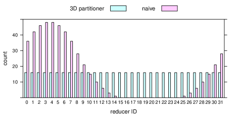
Figure 1: The figure reports the number of reducers in the $i$-th reduce task using a simple partitioner and the one proposed in Algorithm 3 when $\sqrt{n}=32000$, $\sqrt{m}=4000$, and $\rho=8$ (only first round).

4.1 Map and reduce implementation

Map functions are straightforward implementations of the algorithms in Section 3. Reduce functions, while being adherent to the given specifications, present a few caveats from both a correctness and a performance perspective. Reduce functions in Hadoop take input values as instances of the Iterable interface, giving Hadoop developers the freedom of changing the actual underlying implementation without breaking client code. If one needs all the input values at the same time to perform the reduce computation (as is our case), then a deep copy of each value must be saved in local variables or collections to ensure correctness. Simply storing the reference does not work, since the implementation of the Iterable interface used by Hadoop returns a mutable object for each next call (at least in the most recent version, 2.4.0). Failing to perform a deep copy of the input will make the reducer use the same block three times instead of the proper blocks from matrices $A$, $B$, and $C$. Note that by performing this copy we incur an unavoidable performance penalty.

As for the performance in general, it is crucial to use a fast linear algebra library for local multiplications. For the dense case, we use the JBLAS library, that provides Java bindings to the fast BLAS/LAPACK routines. Unfortunately, JBLAS does not support sparse matrices, for which we use MTJ. Although this is the fastest library for sparse matrix multiplication among the tested ones, it is orders of magnitude slower than JBLAS on inputs of the same size thus preventing us to perform complete experiments on sparse matrices.

Partitioner: input: $(i,h,j)$, number of reduce tasks $T$;

      $B$ $\leftarrow$ $\lfloor\rho n/(mT)\rfloor$

      $k$ $\leftarrow$ $i\rho n/m+j\rho+(h\mod\rho)$

      if $z<B\cdot T$ then return $k/B$

      else return Random number in $[0,T)$

     

     

Algorithm 3 Partitioner of the 3D dense algorithm

4.2 Hadoop configuration

As mentioned in Section 2, we used both a in-house cluster and Amazon Web Services (AWS) to carry out our experiments. Our cluster has been configured as follows. HDFS replication has been set to one, that is, redundancy has been disabled. We found that the default replication, 3, degraded performance of $\approx 5\%$ while not providing benefits in our experimental setting. Each machine of the cluster runs two mappers and two reducers, each with 3GB of memory, in order to allow us to use matrix blocks with many elements.

As for the configuration of Hadoop instances provided by AWS, we used the default configuration, customized by Amazon for each machine instance type. The rationale is that AWS provides Hadoop as-a-service, enabling users to concentrate on their application rather than on the configuration and management of an Hadoop cluster.

4.3 Partitioner

The keys of the dense 3D algorithms proposed in the Section 3 are triplets $(i,j,k)$. A partitioner receives as input a key and the number $T$ of reduce tasks in the system and returns the identifier $t\in[0,T)$ of the reduce tasks that will be responsible of the key. When the key is a triplet $(i,j,k)$, a common partitioner for these keys is $t=(31^{2}i+31j+k)\mod T$. However, as Figure 1 shows, this function is not able to evenly distribute reducers among the $T$ reduce tasks.

We propose an alternative partitioner. In the $r$-th round there are $\rho(n/m)$ reducers denoted by keys $(i,h,j)$ with $0\leq i,j<\sqrt{n/m}$ and $(i+j+r\rho)\mod\sqrt{n/m}\leq h<(i+j+(r+1)\rho)\mod\sqrt{n/m}$. The partitioner uniquely maps each key $(i,h,j)$ in the range $[0,\rho n/m)$ by setting $z=i\rho n/m+j\rho+h^{\prime}$ with $h^{\prime}=h\mod\rho$. We note that the mapping consists of a row-major ordering on the first, third and second coordinates, where the second coordinate has been adjusted to be in the range $[0,\rho)$. Keys mapped in $[0,T\lfloor\rho n/(mT)\rfloor)$ are evenly distributed among the reduce tasks, while the remaining at most $T-1$ keys are randomly distributed among the tasks. The pseudocode is given in Algorithm 3. This partitioner is also used in the 3D sparse algorithm, while a slightly different approach is used for the 2D algorithm.

5 Experiments

In this section we propose our experimental analysis of the M₃ library. To better capture the impact of the parameters of the computational model on the performance, we focus on the dense algorithm which heavily loads the communication and computational resources and whose performance does not depend on the particular input matrix. We aim at answering the following questions:

Q1:

How much does the subproblem size $m$ affect the performance?

Q2:

Are the performance of multi-round algorithms comparable with a monolithic algorithm?

Q3:

Which are the major factors affecting the running time?

Q4:

Does the algorithm scale efficiently with processor number?

Q5:

How much is the performance gap between the 2D and 3D approaches?

Q6:

Does the sparse algorithm efficiently exploit the input sparsity?

In Section 5.1 we discuss the results on the in-house cluster. Our claims are also supported by the experiments carried out in the cloud service Amazon Elastic MapReduce and proposed in Section 5.2.

5.1 Experiments on the in-house cluster

In this section we report our investigations on the in-house cluster targeting all of the above questions.

Figure 2: Time vs subproblem size with $\sqrt{n}\in\{16000,32000\}$. The label max (resp., min) means that it has been used maximum (resp., minimum) replication, that is $\rho=\sqrt{n/m}$ (resp., $\rho=1$).

Q1: Impact of subproblem size $m$.

The total amount of shuffled data in all rounds is ${O}\left(n\sqrt{n/m}\right)$. This quantity is independent of the replication factor $\rho$, but increases as $m$ decreases. Since the performance of an algorithm strongly relies on the total amount of shuffled data, it is reasonable to select a large $m$ and then to decompose the problem into larger subproblems. On the other hand, a large value of $m$ reduces parallelism since there are $(n/m)^{3/2}$ independent subproblems. Moreover, it increases the load on each machine since a matrix multiplication of size $\sqrt{m}\times\sqrt{m}$ is computed by each reducer with ${\Theta}\left(m^{3/2}\right)$ work and ${\Theta}\left(m\right)$ memory, which may exceed hardware limits.

This fact is highlighted in Figure 2 which shows the running time for $\sqrt{n}\in\{16000,32000\}$ and $\sqrt{m}\in\{1000,2000,4000\}$; the experiments have been carried out with $\rho=\sqrt{n/m}$ and with $\rho=1$, that is with a monolithic approach and the extreme case of multi-round. All experiments show that the performance improves with larger values of $m$, but the gain decreases for larger values: with input side $\sqrt{n}=32000$ and $\rho=\sqrt{n/m}$, the performance gain when $\sqrt{m}$ moves from $1000$ to $2000$ is $1.99$, while it is $1.12$ when it moves from $2000$ to $4000$. The monolithic approach is slightly less sensible to variations of $m$ since it can exploit much more parallelism in each round than a multi-round approach. The value $\sqrt{m}=8000$ is missing in the experiments since all executions failed due to an out-of-memory error, thus reinforcing the previous claim that larger values of $m$ may exceed hardware limits. Although each submatrix requires 488MB, the actual memory requirements are much more due to the internal structure of Hadoop, which may keep in the memory of each processor the submatrices outputted by map tasks as well as the submatrices required in input by the reduce tasks. Advanced optimizations can increase the maximum value of $m$, but do not significantly change the proposed results.

Q2: Impact of replication factor $\rho$.

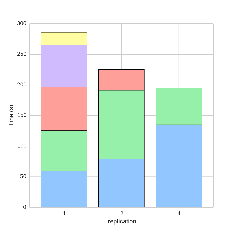
(a) $\sqrt{n}=16000$, $\rho=\{1,2,4\}$.

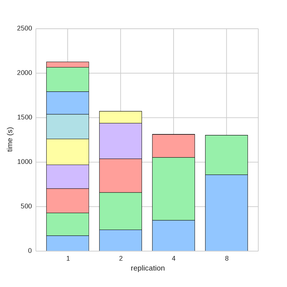
(b) $\sqrt{n}=32000$, $\rho=\{1,2,4,8\}$.

Figure 3: Time vs replication charts. In each bar of the histogram, the $i$-th colored block denotes the time of the $i$-th round.

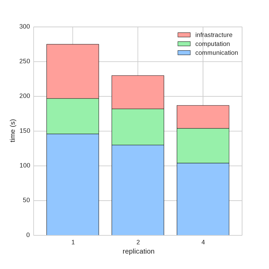
(a) $\sqrt{n}=16000$, $\rho=\{1,2,4\}$.

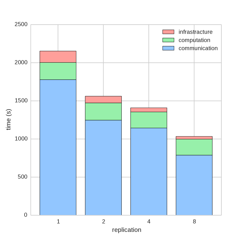
(b) $\sqrt{n}=32000$, $\rho=\{1,2,4,8\}$.

Figure 4: Component cost vs replication. Each bar shows the time of the communication, computation, and infrastructure components.

We are ready to study the performance of a multi-round approach. We recall that, for any replication factor $1\leq\rho\leq\sqrt{n/m}$, the number of rounds is $\sqrt{n}/(\rho\sqrt{m})+1$. Figures 3(a) and 3(b) investigate the running times with different values of the replication factor and input size $\sqrt{n}=16000$ and $\sqrt{n}=32000$, respectively. For $\rho=\sqrt{n/m}$, we get a monolithic approach (i.e., two rounds). Without any surprise, the best running time is reached by the monolithic approach: this supports the common practice to minimize round number, but only if the total amount of communication remains unchanged. However, we observe that a multi-round approach increases the running time with respect to the monolithic two-round approach by an average factor $7\%$ for each additional round. We believe that the main reason of this increase is due to the distributed file system HDFS, which is used for storing pairs between rounds and is optimized for writing and reading large files. When $\rho=\sqrt{n/m}$, each reduce task writes two large chunks of output pairs (one per round) on HDFS containing all outputs of the associated reducers in a given round. On the other hand, for values of $\rho$ smaller than $\sqrt{n/m}$, each reduce task writes a larger number of chunks of smaller size. Although the total size of the written files is the same in each approach, the system is not able to exploit the features of HDFS with a multi-round approach. We conjecture that the performance gap can be closed by exploiting other implementations that use local file systems for storing intermediate pairs (e.g., Spark).

Figures 3(a) and 3(b) also show the running time of each round: for each histogram bar, the $i$-th colored block from the bottom denotes the time of the $i$-th round. The work is evenly distributed among rounds and the cost of each round decreases with the replication factor $\rho$. In each run, the last round is faster than the remaining ones since the reduce function only performs the addition of $\rho$ submatrices. Finally, we observe that the algorithm efficiently scales with the input size: the running time, for any replication factor, increases on the in-house cluster by a factor $\sim 8$ when the input side doubles, which agrees with the cubic (in the matrix side) complexity of the algorithm.

Q3: Cost analysis.

We now analyze how communication, computation and infrastructure affect the running time. We define the following three costs:

• Infrastructure cost $T_{infr}$: It is the time for setting up the Hadoop system and each round. It is given by the time of the algorithm when no computation is done in the reduce functions and the value of each pair is replaced by an empty matrix (i.e., the amount of shuffled data is negligible).

• Computation cost $T_{comp}$: It is the time for performing the local computation. Let $\hat{T}_{comp}$ be the time of the algorithm when any local multiplication is performed on two locally created matrices (the cost of the creation is negligible) and the value of each pair is replaced by an empty matrix. Then, the computation cost is $\hat{T}_{comp}-T_{infr}$.

• Communication cost $T_{comm}$: It is the time for exchanging pairs between mappers and reducers, and includes the costs of reading/writing data on HDFS and of shuffle steps. Let $\hat{T}_{comm}$ be the time of the algorithm when no computation is done in the reduce function (the output pair is a copy of an input pair). Then, the communication cost is $\hat{T}_{comm}-T_{infr}$.
  

We think that the infrastructure cost is a good approximation of the true time for setting up the system and each round. However, this is not true for the communication and computation costs since the procedure does not take into account the concurrency between the three components. Nevertheless, these costs still provide an interesting overview of the main factors determining the running time of an algorithm. (To the best of our knowledge no tools for cost analysis are available.) Figures 4(a) and 4(b) show the costs of the three components for $\sqrt{n}=16000$ and $\rho\in\{1,2,4\}$, and for $\sqrt{n}=32000$ and $\rho\in\{1,2,4,8\}$, respectively. The infrastructure cost increases linearly with the round number, and the average fixed cost of a round is $17$ seconds. The computation cost for a given input size is independent of the replication value, which confirms that the work is evenly distributed among cluster nodes. The communication cost increases when $\rho$ increases as already noted for Figures 3(a) and 3(b), and dominates the total time.

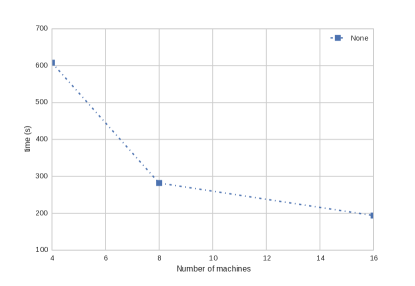
Figure 5: Time vs number of nodes with $\sqrt{n}=16000$. The experiments have been carried out with replication $\rho\in\{1,2,4\}$ and $p\in\{4,8,16\}$ nodes.

Q4: Scalability.

We now study the scalability of the algorithm by running the dense algorithm on a smaller number of nodes. For this experiment, we run the dense algorithm with input size 16000 on 4, 8 and 16 nodes of the in-house cluster. The results are given in Figure 5 with different replication factors $\rho\in\{1,2,4\}$. The algorithm scales efficiently although there is a small reduction in the speed up with 16 nodes. This may be due to a loss in data locality and to a larger cost of the shuffle step when the algorithm is run on 16 nodes.

Q5: 2D vs. 3D algorithms

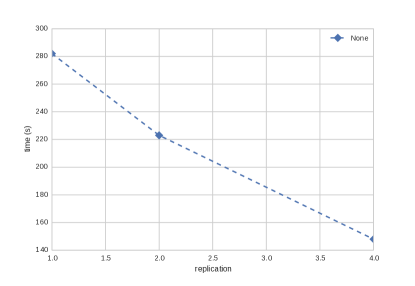
Figure 6: Comparison between the 2D and 3D approaches with $\sqrt{n}=16000$. The replication factor is $\rho\in\{1,2,4\}$ for the 3D approach, and $\rho\in\{1,2,4,8,16\}$ for the 2D approach.

We now move to analyze the performance of the 3D multiplication strategy compared with the 2D strategy. Figure 6 clearly shows that the 3D approach has a significant performance advantage. This is due to the fact that the total shuffle size is, for the 3D approach, ${O}\left(n\sqrt{n/m}\right)$, whereas for the 2D approach it is ${O}\left(n^{2}/m\right)$. Since the major bottleneck in MapReduce is communication, the 2D approach incurs a significant penalty.

Q6: Sparse matrices.

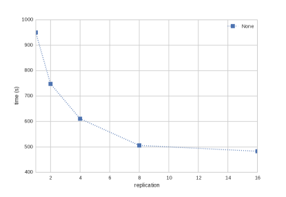
Figure 7: Time vs replication for sparse matrix multiplication with $\sqrt{n}\in\{2^{20},2^{22},2^{24}\}$ and an average of 8 non-zero entries per row and per column. For each input size, we consider all possible replication factors, from 0 to $\sqrt{n}/\sqrt{m^{\prime}}$ ($\sqrt{m^{\prime}}$ is set to $\{2^{18},2^{19},2^{20}\}$, respectively).

We now investigate the performance of the 3D sparse algorithm and show that it improves performance by exploiting input sparsity. Figure 7 shows the running times with different replication factors of the 3D sparse algorithm with two input Erdös-Rényi matrices with $\sqrt{n}\in\{2^{20},2^{22},2^{24}\}$, and an average of 8 non-zero entries per row and per column (i.e., $\delta\in\{1/2^{17},1/2^{19},1/2^{21}\}$, respectively). Since the output matrices have expected density $\delta_{O}\in\{1/2^{14},1/2^{16},1/2^{18}\}$ (see Section 2), the input matrices are partitioned into submatrices of size $2^{18}$, $2^{19}$ and $2^{20}$, respectively, so that the expected number of non-zero elements in each submatrix of the output is comparable with the subproblem size of the dense case. This shows that, by exploiting the sparseness of the input matrix, we can tackle much bigger problems, under the same memory constraints. As mentioned in Section 4, we avoided the computation of local products because of the lack of an efficient Java implementation of sequential sparse matrix multiplication. However, as we have experimentally shown, the time spent computing local products is a fixed additive factor, whereas the communication is the dominant component, thus these experiments clearly show the tradeoffs between round number and time for sparse matrix multiplication.

5.2 Experiments on Amazon Elastic MapReduce

In this section we report our investigations in Amazon Elastic MapReduce (EMR) targeting the questions Q1, Q2 and Q3 described at the beginning of Section 5.

Q1: Impact of subproblem size $m$.

These experiments show a similar behavior on c3.8xlarge and i2.xlarge instances, with $\sqrt{m}=4000$ being the optimal choice. Interestingly, smaller instance types (like c3.xlarge) require $\sqrt{m}=2000$ for avoiding memory errors. All the following experiments assume $\sqrt{m}=4000$.

Q2: Impact of replication factor $\rho$.

The experiments have been carried out on EMR with c3.8xlarge instances and the results are in Figures 8 and 10(a) with $\sqrt{n}\in\{16000,32000\}$, respectively. Running times significantly increase with respect to experiments on the in-house cluster: the running times with $\sqrt{n}=16000$ (resp., $\sqrt{n}=32000$) on EMR are on the average $4.7$ (resp., $1.4$) times larger than the ones on the in-house cluster, even if the computational resources of the two systems are somewhat similar. It is interesting to note that the gap decreases with larger input sizes. The average performance loss with respect to the monolithic two-round approach is $17\%$ for each additional round.

As for the scalability, we observe that the scaling factor on EMR is $\sim 5$, smaller than the one achieved on the in-house cluster ($\sim 8$). This is due to high fixed costs which are not efficiently amortized with small inputs.

Q3: Cost analysis.

The cost analysis on EMR with c3.8xlarge instances is reported in Figures 9(a) and 10(b) for $\sqrt{n}=16000$ and $\rho\in\{1,2,4\}$, and for $\sqrt{n}=32000$ and $\rho\in\{1,2,4,8\}$, respectively. It should be noted that the average computation cost is similar to the respective component in the in-house cluster, although there is a larger variance due to the unpredictable load of the physical machines of EMR. The average infrastructure cost is 30 seconds.

Finally, we report in Figure 9(b) the cost analysis with $\sqrt{n}=16000$ and $\rho\in\{1,2,4\}$ on i2.xlarge instances. A i2.xlarge instance has faster disks optimized for random I/Os but slower network than a c3.8xlarge instance. However, we observe that the communication costs are smaller than the respective costs in Figure 9(a) for c3.8xlarge instances. This fact supports the claim in Section 5.1 (question Q2) that the main bottleneck is the inability of HDFS to efficiently read/write small chunks of data.

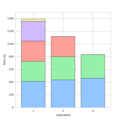
Figure 8: Time vs replication with $\sqrt{n}=16000$ and $\rho=\{1,2,4\}$ on c3.8xlarge instances. In each bar of the histogram, the $i$-th colored block denotes the time of the $i$-th round.

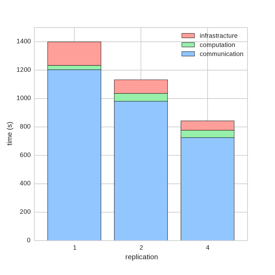
(a) Component cost vs replication with $\sqrt{n}=16000$, $\rho=\{1,2,4\}$ on c3.8xlarge instances. Each bar shows the time of the communication, computation, and infrastructure components.

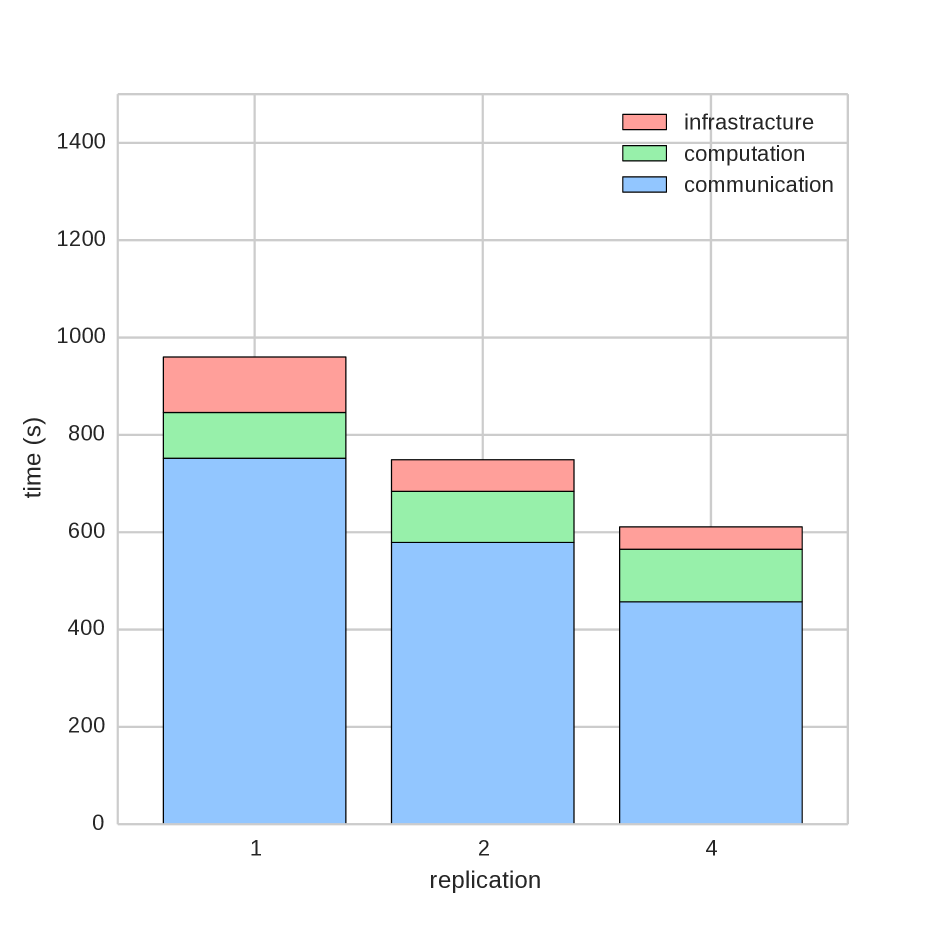
(b) Component cost vs replication with $\sqrt{n}=16000$, $\rho=\{1,2,4\}$ on i2.xlarge instances. Each bar shows the time of the communication, computation, and infrastructure components.

Figure 9: Component cost for multiplying $16000\times 16000$ matrices on Amazon EMR, using different instance types. Instances of type i2.xlarge (Figure 9(b)) have a faster disk with respect to c3.8xlarge instances (Figure 9(a)).

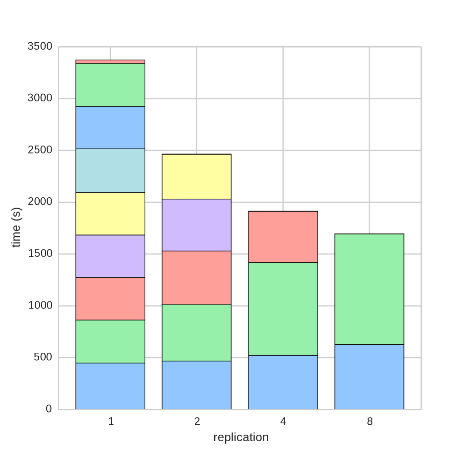
(a) Time vs replication with $\sqrt{n}=32000$, $\rho=\{1,2,4,8\}$ on c3.8xlarge instances. In each bar of the histogram, the $i$-th colored block denotes the time of the $i$-th round.

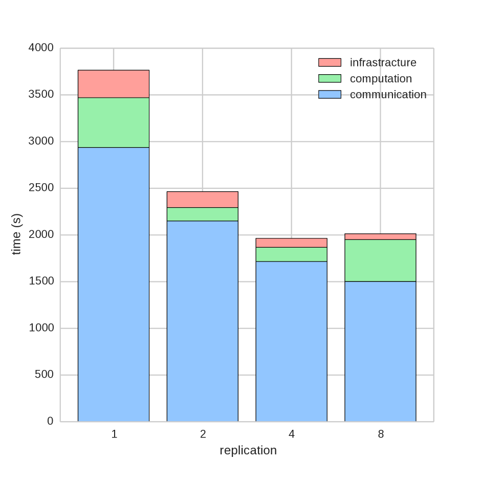
(b) Component cost vs replication with $\sqrt{n}=32000$ and $\rho=\{1,2,4,8\}$ on c3.8xlarge instances. Each bar shows the time of the communication, computation, and infrastructure components.

Figure 10: Experiments on Amazon EMR for multiplying $32000\times 32000$ dense matrices.

6 Conclusion

In this paper we have proposed the Hadoop library M₃ for performing dense and sparse matrix multiplication in MapReduce by exploiting the theoretical results in [16], and we have carried out an extensive experimental study on an in-house cluster and Amazon Web Services. The results give evidence that multi-round algorithms can have performance comparable with monolithic ones (assuming a similar total amount of communication) even on the Hadoop framework, which is not the most suitable MapReduce implementation for executing multi-round algorithms. Moreover, experiments suggest that the common attitude to only focus on round number when designing MapReduce algorithms could significantly reduce performance if it implies a larger amount of total communication. This fact supports recent computational models for MapReduce that mainly focus on the minimization of the total communication complexity [8], or that aim at reducing round number when an upper bound on the allowed total communication complexity is given [16].

As future work, we plan to further investigate sparse matrix multiplication on MapReduce and to test our algorithms on other implementations of the MapReduce paradigm. In particular, we are currently developing our algorithms in the Spark framework, where the management of the input/output pairs of each round is more efficient than Hadoop.

References

- [1] Foto N. Afrati, Magdalena Balazinska, Anish Das Sarma, Bill Howe, Semih Salihoglu, and Jeffrey D. Ullman. Designing good algorithms for MapReduce and beyond. In Proc. 3rd SoCC, pages 26:1–26:2, 2012.
- [2] Foto N. Afrati, Anish Das Sarma, Semih Salihoglu, and Jeffrey D. Ullman. Upper and lower bounds on the cost of a Map-Reduce computation. Proc. VLDB Endow., 6(4):277–288, 2013.
- [3] Grey Ballard, Aydin Buluc, James Demmel, Laura Grigori, Benjamin Lipshitz, Oded Schwartz, and Sivan Toledo. Communication optimal parallel multiplication of sparse random matrices. In Pro. 25th ACM SPAA, pages 222–231, 2013.
- [4] Aydin Buluç and John R. Gilbert. Parallel sparse matrix-matrix multiplication and indexing: Implementation and experiments. SIAM J. Scientific Computing, 34(4), 2012.
- [5] Matteo Ceccarello, Andrea Pietracaprina, Geppino Pucci, and Eli Upfal. Parallel graph decomposition and diameter approximation in o(diameter) time and linear space. arXiv 1407.3144.
- [6] Jeffrey Dean and Sanjay Ghemawat. MapReduce: Simplified data processing on large clusters. Commun. ACM, 51(1):107–113, 2008.
- [7] Gene H. Golub and Charles F. Van Loan. Matrix Computations. Matrix Computations. Johns Hopkins University Press, 2012.
- [8] Michael Goodrich, Nodari Sitchinava, and Qin Zhang. Sorting, searching, and simulation in the MapReduce framework. In Proc. 22nd ISAAC, pages 374–383, 2011.
- [9] Robert L. Grossman and Yunhong Gu. Data mining using high performance data clouds: experimental studies using sector and sphere. KDD, 2008.
- [10] Howard Karloff, Siddharth Suri, and Sergei Vassilvitskii. A model of computation for MapReduce. In Proc. 21 SODA, pages 938–948, 2010.
- [11] Jimmy Lin and Chris Dyer. Data-intensive Text Processing with MapReduce. Morgan & Claypool, 2010.
- [12] Jimmy Lin and Michael Schatz. Design patterns for efficient graph algorithms in MapReduce. In Proc. 8th MLG, pages 78–85, 2010.
- [13] Sean Owen, Robin Anil, Ted Dunning, and Ellen Friedman. Mahout in Action. Manning Publications Co., 2011.
- [14] Rasmus Pagh and Morten Stöckel. The input/output complexity of sparse matrix multiplication. In Proc. 22nd ESA, pages 750–761, 2014.
- [15] Ha-Myung Park, Francesco Silvestri, U Kang, and Rasmus Pagh. MapReduce triangle enumeration with guarantees. In Proc. 23rd CIKM, 2014.
- [16] Andrea Pietracaprina, Geppino Pucci, Matteo Riondato, Francesco Silvestri, and Eli Upfal. Space-round tradeoffs for MapReduce computations. In Proc. 26th ICS, pages 235–244, 2012.
- [17] Steven J. Plimpton and Karen D. Devine. MapReduce in MPI for large-scale graph algorithms. Parallel Comput., 37(9):610–632, 2011.
- [18] Sangwon Seo, E.J. Yoon, Jaehong Kim, Seongwook Jin, Jin-Soo Kim, and Seungryoul Maeng. HAMA: An efficient matrix computation with the MapReduce framework. In Proc. of 2nd CloudCom, pages 721–726, 2010.
- [19] Konstantin Shvachko, Hairong Kuang, Sanjay Radia, and Robert Chansler. The hadoop distributed file system. In Proc. 26th MSST, pages 1–10, 2010.
- [20] Satish Narayana Srirama, Pelle Jakovits, and Eero Vainikko. Adapting scientific computing problems to clouds using MapReduce. Future Generation Computer Systems, 28(1):184 – 192, 2012.
- [21] Ronald Taylor. An overview of the Hadoop/MapReduce/ HBase framework and its current applications in bioinformatics. BMC Bioinformatics, 11(Suppl 12):S1+, 2010.
- [22] Tom White. Hadoop: The definitive guide. O’Reilly Media, Inc., 2012.
- [23] Matei Zaharia, Mosharaf Chowdhury, Michael J. Franklin, Scott Shenker, and Ion Stoica. Spark: Cluster computing with working sets. In Proc. 2Nd USENIX HotCloud, pages 10–10, 2010.