Models of the circumstellar medium of evolving, massive runaway stars moving through the Galactic plane

Abstract

At least 5 per cent of the massive stars are moving supersonically through the interstellar medium (ISM) and are expected to produce a stellar wind bow shock. We explore how the mass loss and space velocity of massive runaway stars affect the morphology of their bow shocks. We run two-dimensional axisymmetric hydrodynamical simulations following the evolution of the circumstellar medium of these stars in the Galactic plane from the main sequence to the red supergiant phase. We find that thermal conduction is an important process governing the shape, size and structure of the bow shocks around hot stars, and that they have an optical luminosity mainly produced by forbidden lines, e.g. [O iii]. The H$\alpha$ emission of the bow shocks around hot stars originates from near their contact discontinuity. The H$\alpha$ emission of bow shocks around cool stars originates from their forward shock, and is too faint to be observed for the bow shocks that we simulate. The emission of optically-thin radiation mainly comes from the shocked ISM material. All bow shock models are brighter in the infrared, i.e. the infrared is the most appropriate waveband to search for bow shocks. Our study suggests that the infrared emission comes from near the contact discontinuity for bow shocks of hot stars and from the inner region of shocked wind for bow shocks around cool stars. We predict that, in the Galactic plane, the brightest, i.e. the most easily detectable bow shocks are produced by high-mass stars moving with small space velocities.

1 Introduction

Massive stars have strong winds and evolve through distinct stellar evolutionary phases which shape their surroundings. Releasing material and radiation, they give rise to ISM structures whose geometries strongly depend on the properties of their driving star, e.g. rotation (Langer et al., 1999; van Marle et al., 2008; Chita et al., 2008), motion (Brighenti & D’Ercole, 1995a, b), internal pulsation (see chapter 5 in van Veelen, 2010), duplicity (Stevens et al., 1992) or stellar evolution (e.g. the Napoleon’s hat generated by the progenitor of the supernova SN1987A and overhanging its remnant, see Wang et al., 1993). At the end of their lives, most massive stars explode as a supernova or generate a gamma-ray burst event (Woosley et al., 2002) and their ejecta interact with their circumstellar medium (Borkowski et al., 1992; van Veelen et al., 2009; Chiotellis et al., 2012). Additionally, massive stars are important engines for chemically enriching the interstellar medium (ISM) of galaxies, e.g. via their metal-rich winds and supernova ejecta, and returning kinetic energy and momentum to the ISM (Vink, 2006).

Between 10 and 25 per cent of the O stars are runaway stars (Gies, 1987; Blaauw, 1993) and about 40 per cent of these, i.e. about between 4 and 10 per cent of all O stars (see Huthoff & Kaper, 2002), have identified bow shocks. The bow shocks can be detected at X-ray (López-Santiago et al., 2012), ultraviolet (Le Bertre et al., 2012), optical (Gull & Sofia, 1979), infrared (van Buren & McCray, 1988a) and radio (Benaglia et al., 2010) wavelengths. The bow-shock-producing stars are mainly on the main sequence or blue supergiants (van Buren et al., 1995; Peri et al., 2012). There are also known bow shocks around red supergiants, Betelgeuse (Noriega-Crespo et al., 1997; Decin et al., 2012), $\mu$ Cep (Cox et al., 2012) and IRC$-$10414 (Gvaramadze et al., 2014) or asymptotic giant branch stars (Cox et al., 2012; Jorissen et al., 2011). Bow shocks are used to find new runaway stars (Gvaramadze, Kroupa & Pflamm-Altenburg, 2010), to identify star clusters from which these stars have been ejected (Gvaramadze & Bomans, 2008) and to constrain the properties of their central stars, e.g. mass-loss rate (Gull & Sofia, 1979; Gvaramadze et al., 2012), or the density of the local ISM (Kaper et al., 1997; Gvaramadze et al., 2014).

The structure of such bow shocks is sketched in Fig. 1. However the layers of shocked ISM develop differently as a function of the wind power and ISM properties. The wind and ISM pressure balance at the contact discontinuity. It separates the regions of shocked material bordered by the forward and reverse shocks. The distance from the star to the contact discontinuity in the direction of the relative motion between wind and ISM defines the stand-off distance of the bow shock (Baranov, Krasnobaev & Kulikovskii, 1971). The shape of isothermal bow shocks, in which the shocked regions are thin, is analytically approximated in Wilkin (1996).

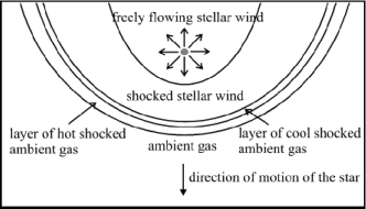
Figure 1: Typical structure of a bow shock generated by a hot runaway star. The figure is taken from Comerón & Kaper (1998).

A numerical study by Comerón & Kaper (1998) compares wind-ISM interactions with (semi-)analytical models and concludes that the thin-shell approximation has partial validity. This work describes the variety of shapes which could be produced in bow shocks of OB stars. It details how the action of the wind on the ISM, together with the cooling in the shocked gas, shapes the circumstellar medium, determines the relative thickness of the layers composing a bow shock, and determines its (in)stability. It shows the importance of heat conduction (Spitzer, 1962; Cowie & McKee, 1977) to the size of these bow shocks, and that rapid cooling distorts them. The shocked regions are thick if the shock is weak, but they cool rapidly and become denser and thinner for the regime involving either high space velocities or strong winds and/or high ambient medium densities. This leads to distorting instabilities such as the transverse acceleration instability (Blondin & Koerwer, 1998) or the non-linear thin shell instability (Dgani et al., 1996a, b). Mac Low et al. (1991) models bow shocks around main sequence stars in dense molecular clouds. The bow shock models in Comerón & Kaper (1998) are set in low-density ambient medium.

Models for bow shocks around evolved, cool runaway stars exist for several stellar evolutionary phases, such as red supergiants (Brighenti & D’Ercole, 1995a; Mohamed et al., 2012; Decin et al., 2012) or asymptotic giant branch (AGB) phases (Wareing et al., 2007a; Villaver et al., 2012). When a bow shock around a red supergiant forms, the new-born shell swept up by the cool wind succeeds the former bow shock from the main sequence. A collision between the old and new shells of different densities precedes the creation of a second bow shock (Mackey et al., 2012). Bow shocks around cool stars are more likely to generate vortices (Wareing et al., 2007b) and their substructures are Rayleigh-Taylor and Kelvin-Helmholtz unstable (Decin et al., 2012). The dynamics of ISM dust grains penetrating into the bow shocks of red supergiants is numerically investigated in van Marle et al. (2011). The effect of the space velocity and the ISM density on the morphology of Betelgeuse’s bow shock is explored in Mohamed et al. (2012), however this study considers a single mass-loss rate and does not allow to appreciate how the wind properties modify the bow shock’s shape or luminosity. In addition, van Marle et al. (2014) show the stabilizing effect of a weak ISM magnetic field on the bow shock of Betelgeuse.

In this study, we explore in a grid of 2D models the combined role of the star’s mass-loss and its space velocity on the dynamics and morphology of bow shocks of various massive stars moving within the Galactic plane. We use representative initial masses and space velocities of massive stars (Eldridge, Langer & Tout, 2011). Stellar evolution is followed from the main sequence to the red supergiant phase. The treatment of the dissipative processes and the discrimination between wind and ISM material allows us to calculate the bow shock luminosities and to discuss the origin of their emission. We also estimate the luminosity of the bow shocks to predict the best way to observe them. The project differs from previous studies (e.g. Comerón & Kaper, 1998; Mohamed et al., 2012) in that we use more realistic cooling curves, we include stellar evolution in the models and because we focus on the emitting properties and observability of our bow shocks. We do not take into account the inhomogeneity and the magnetic field of the ISM.

This paper is organised as follows. We first begin our Section 2 by presenting our method, stellar evolution models, included physics and the numerical code. Models for the main sequence, the stellar phase transition and red supergiant phases are presented in Sections 3, 4 and 5, respectively. We describe the grid of 2D simulations of bow shocks around massive stars, discuss their morphology, compare their substructures to an analytical solution for infinitely thin bow shock and present their luminosities and H$\alpha$ surface brightnesses. Section 6 discusses our results. We conclude in Section 7.

2 Numerical scheme and initial parameters

2.1 Hydrodynamics, boundary conditions and numerical scheme

The governing equations are the Euler equations of classical hydrodynamics, including radiative cooling and heating for an optically-thin plasma and taking into account electronic thermal conduction, which are,

$$\frac{\partial\rho}{\partial t}+\mn@boldsymbol{\nabla}\cdot(\rho\mn@boldsymbol{v})=0,$$ (1)

$$\frac{\partial\rho\mn@boldsymbol{v}}{\partial t}+\mn@boldsymbol{\nabla}\cdot(\mn@boldsymbol{v}\otimes\rho\mn@boldsymbol{v})+\mn@boldsymbol{\nabla}p=\mn@boldsymbol{0},$$ (2)

and,

$$\frac{\partial E}{\partial t}+\mn@boldsymbol{\nabla}\cdot(E\mn@boldsymbol{v})+\mn@boldsymbol{\nabla}\cdot(p\mn@boldsymbol{v})=\mathit{\Phi}(T,\rho)+\mn@boldsymbol{\nabla}\cdot\mn@boldsymbol{{F}_{\rm c}}.$$ (3)

In the system of equations (1)$-$(3), $\mn@boldsymbol{v}$ is the gas velocity in the frame of reference of the star, $\rho$ is the gas mass density and $p$ is its thermal pressure. The total number density $n$ is defined by $\rho=\mu nm_{\rm H}$, where $\mu$ is the mean molecular weight in units of the mass of the hydrogen atom $m_{\rm H}$. The total energy density is the sum of its thermal and kinetic parts,

$$E=\frac{p}{(\gamma-1)}+\frac{\rho v^{2}}{2},$$ (4)

where $\gamma$ is the ratio of specific heats for an ideal gas, i.e. $\gamma=5/3$. The temperature inside a given layer of the bow shock is given by,

$$T=\mu\frac{m_{\mathrm{H}}}{k_{\rm{B}}}\frac{p}{\rho},$$ (5)

where $k_{\rm B}$ is the Boltzmann constant. The quantity $\it\Phi$ in the energy equation (3) gathers the rates $\it\Lambda$ for optically-thin radiative cooling and $\it\Gamma_{\alpha}$ for heating,

$$\mathit{\Phi}(T,\rho)=n^{\alpha}_{\mathrm{H}}\mathit{\Gamma}_{\alpha}(T)-n^{2}_{\mathrm{H}}\mathit{\Lambda}(T),$$ (6)

where the exponent $\alpha$ depends on the ionization of the medium (see Section 2.4), and $n_{\rm H}$ is the hydrogen number density. The heat flux is symbolised by the vector $\mn@boldsymbol{F_{\rm c}}$. The relation $c_{\rm s}=\sqrt{\gamma p/\rho}$ closes the system of partial differential equations (1)$-$(3), where $c_{\rm s}$ is the adiabatic speed of sound.

We perform calculations on a 2D rectangular computational domain in a cylindrical frame of reference $(O;R,z)$ of origin $O$, imposing rotational symmetry about $R=0$. We use a uniform grid divided into $N_{\rm R}\times N_{\rm z}$ cells, and we pay attention to the number of cells resolving the layers of the bow shocks (Comerón & Kaper, 1998). We choose the size of the computational domain such that the tail of the bow shock only crosses the downstream boundary $z=z_{\rm min}$. Following the methods of Comerón & Kaper (1998) and van Marle et al. (2006), a stellar wind is released into the domain by a half circle of radius $20$ cells centred on the origin. We impose at every timestep a wind density $\rho_{\rm w}\propto r^{-2}$ onto this circle, where $r$ is the distance to $O$. We work in the frame of reference of the runaway star. Outflow boundary conditions are assigned at the $z=z_{\rm min}$ and $R=R_{\rm max}$ borders of the domain, whereas ISM material flows into the domain from the $z=z_{\rm max}$ border. The choice of a 2D cylindrical coordinate system possessing an intrinsic axisymmetric geometry limits us to the modelling of symmetric bow shocks only.

We solve the equations with the magneto-hydrodynamics code pluto  (Mignone et al., 2007, 2012). We use a finite volume method with the Harten-Lax-van Leer approximate Riemann solver for the fluid dynamics, controlled by the standard Courant-Friedrich-Levy (CFL) parameter initially set to $C_{\rm cfl}=0.1$. The equations are integrated with a second order, unsplit, time-marching algorithm. This Godunov-type scheme is second order accurate in space and in time. Optically-thin radiative losses are linearly interpolated from tabulated cooling curves and the corresponding rate of change is subtracted from the pressure. The parabolic term in the equation (3), corresponding to the heat conduction is treated with the Super-Time-Stepping algorithm (Alexiades et al., 1996) in an operator-split, first order accurate in time algorithm.

We use pluto 4.0 where linear interpolation in cylindrical coordinates is correctly performed by taking into account the geometrical centroids rather than the cell centre (Mignone, 2014). We have found that this leads to better results compared to pluto 3.1, especially in close proximity to the axis. The diffusive solver chosen to carry out the simulations damps the dramatic numerical instabilities along the symmetry axis at the apex of the bow shocks (Vieser & Hensler, 2007; Kwak et al., 2011) and is more robust for hypersonic flows. All the physical components of the model are included from the first timestep of the simulations.

2.2 Wind model

Stellar evolution models provide us with the wind parameters throughout the star’s life from the main sequence to the red supergiant phase (see evolutionary tracks in Fig. 2). We obtain the wind inflow boundary conditions from a grid of evolutionary models for non-rotating massive stars with solar metallicity (Brott et al., 2011). Their initial masses are $M_{\star}=10,20$ and $40\,\mathrm{M}_{\odot}$ (the masses of the stars quoted hereafter are the zero-age main sequence masses, unless otherwise stated), and they have been modelled with the Binary Evolution Code (BEC) (Heger et al., 2000; Yoon & Langer, 2005) including mass-loss but ignoring overshooting. The mass-loss rate calculation includes the prescriptions for O-type stars by Vink et al. (2000, 2001) and for cool stars by de Jager et al. (1988).

Fig. 3 shows the stellar wind properties of the different models at a radius of $r=0.01\,\mathrm{pc}$ from the star. Mass-loss rate $\dot{M}$, wind density $\rho_{w}$ and velocity $v_{\rm w}$ are linked by,

$$\rho_{w}=\frac{\dot{M}}{4\pi r^{2}v_{\rm w}}.$$ (7)

The wind terminal velocity is calculated from the escape velocity $v_{\mathrm{esc}}$ using $v_{\rm w}^{2}=\beta_{w}(T)v_{\mathrm{esc}}^{2}$ (Eldridge et al., 2006), with $\beta_{w}$ a parameter given in their table 1.

The mass-loss rate of the star has a constant value of around $10^{-9.5}$, $10^{-7.3}$ and $10^{-6.2}\,\mathrm{M}_{\odot}\,\mathrm{yr}^{-1}$ during the main sequence phase of the $10,\,20$ and $40\,\mathrm{M}_{\odot}$ stars, respectively. After the transition to a red supergiant, the mass-loss increases to around $10^{-6.2}$ and around $10^{-5}\,\mathrm{M}_{\odot}\,\mathrm{yr}^{-1}$ for the $10\,\mathrm{M}_{\odot}$ and $20\,\mathrm{M}_{\odot}$ stars, respectively. The evolutionary model of our $40\,\mathrm{M}_{\odot}$ star ends at the beginning of the helium ignition, i.e. it does not have a red supergiant phase (Brott, private communication). Such a star may evolve through the red supergiant phase but this is not included in our model (see panel (f) of Fig. 3). The wind velocity decreases by two orders of magnitude from $\sim\,1000\,\mathrm{km}\,\mathrm{s}^{-1}$ during the main sequence phase to $\sim\,10\,\mathrm{km}\,\mathrm{s}^{-1}$ for the red supergiant phase. The effective temperature of the star decreases from $T_{\mathrm{eff}}\sim 10^{4}\,\mathrm{K}$ during the main sequence phase to $T_{\mathrm{eff}}\sim 2.5$$-$$4.5\times 10^{3}\,\mathrm{K}$ when the star becomes a red supergiant. The thermal pressure of the wind is proportional to $T_{\mathrm{eff}}$, according to the ideal gas equation of state. It scales as $r^{-2\gamma}$ and is negligible during all evolutionary phases compared to the ram pressure of the wind in the free expanding region.

We run two simulations for each $M_{\star}$ and for each considered space velocity $v_{\star}$: one for the main sequence and one for the red supergiant phase. Simulations are launched at $5$ and $3\,\rm Myr$ of the main sequence phase for the $10$ and $20\,\mathrm{M}_{\odot}$ models, and at the zero-age main-sequence for the $40\,\mathrm{M}_{\odot}$ star, given its short lifetime (see black circles in Figs. 2 and 3). Red supergiant simulations are started before the main sequence to red supergiant transition such that a steady state has been reached when the red supergiant wind begins to expand (see black squares in Figs. 2 and 3).

The wind material is traced using a scalar marker whose value $Q$ obeys the linear advection equation,

$$\frac{\partial(\rho Q)}{\partial t}+\mn@boldsymbol{\nabla}\cdot(\mn@boldsymbol{v}\rho Q)=0.$$ (8)

This tracer is passively advected with the fluid, allowing us to distinguish between the wind and ISM material. Its value is set to $Q(\mn@boldsymbol{r})=1$ for the inflowing wind material and to $Q(\mn@boldsymbol{r})=0$ for the ISM material, where $\mn@boldsymbol{r}$ is the vector position of a given cell of the simulation domain.

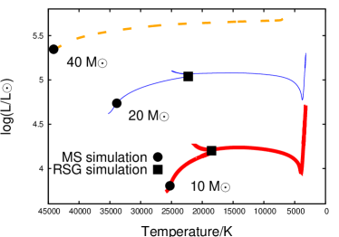
Figure 2: Stellar evolutionary tracks used in the simulations. Thick solid red line, thin solid blue line and dashed orange line are the evolutionary tracks for our $10$, $20$ and $40$ $\mathrm{M}_{\odot}$ models, respectively. Circles indicate the time of the beginning of the simulations for the main sequence phase and squares for the red supergiant phase.

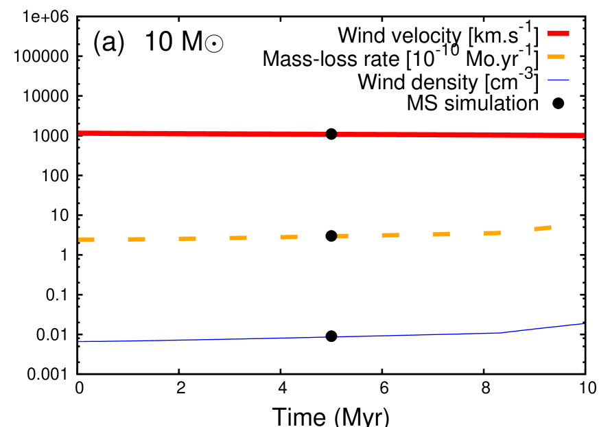
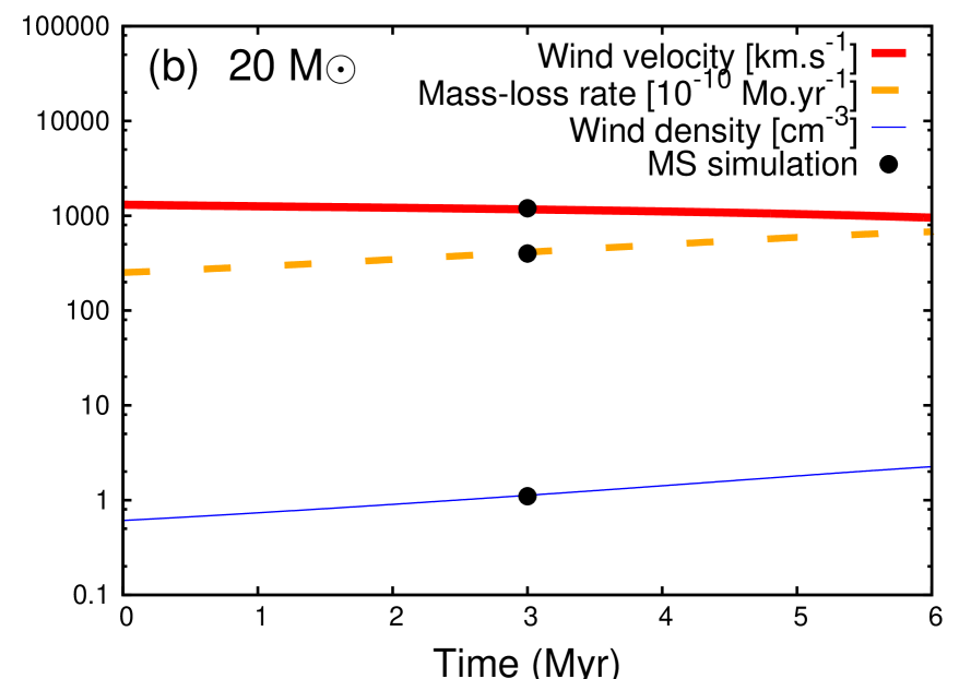
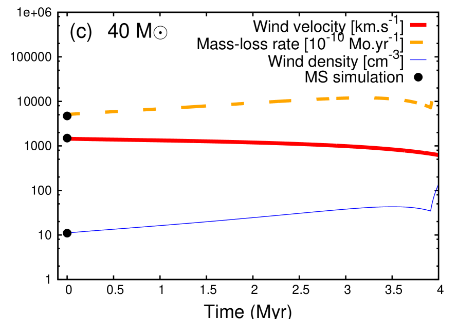
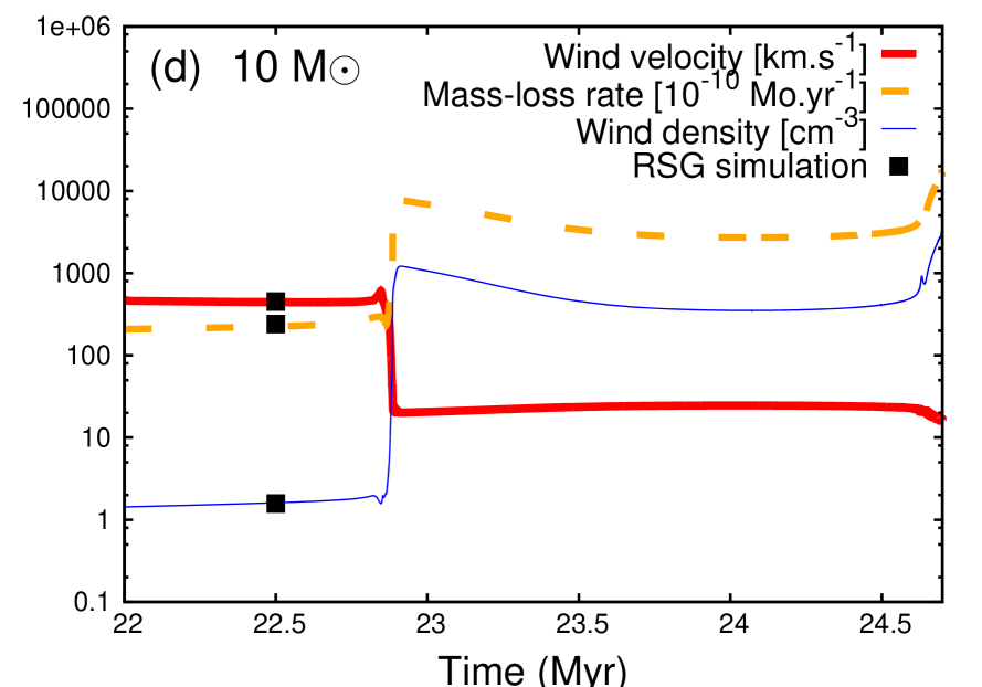
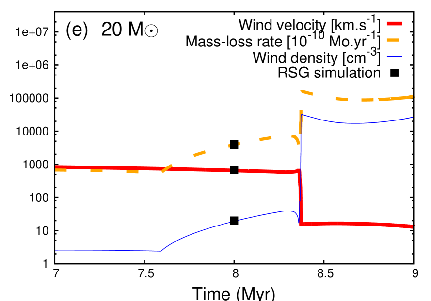
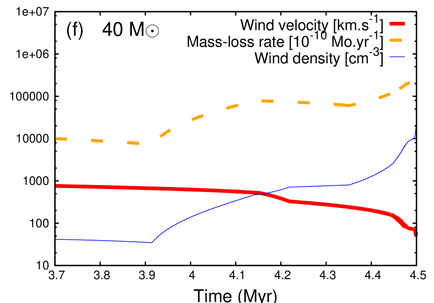
Figure 3: Physical parameters of the stellar winds used in our simulations. The top panels represent the wind velocity $v_{\mathrm{w}}$ (thick solid red line), the mass-loss rate $\dot{M}$ (dashed orange line) and the wind number density $n_{\mathrm{w}}$ (thin solid blue line) during the main sequence phase of the $10$, $20\,\mathrm{and}\,40\,\mathrm{M_{\odot}}$ stars, whereas the bottom panels show these parameters during the red supergiant phase of the same stars. Wind number density is calculated at $0.01\,\mathrm{pc}$ from the star and are proportional to the mass-loss rate $\dot{M}$ (see Eq. 7). Black dots show the beginning of the simulations for the main sequence phase and black squares for the red supergiant phase (Table 1).

2.3 Interstellar medium

We consider homogeneous and laminar ISM with $n_{\rm H}=0.57\,\mathrm{cm}^{-3}$, which is typical of the warm neutral medium in the Galactic plane (Wolfire et al., 2003) from where most of runaway massive stars are ejected. The initial ISM gas velocity is set to $v_{\mathrm{ISM}}=-v_{\star}$.

The photosphere of a main sequence star releases a large flux of hydrogen ionizing photons $S_{\star}$, that depends on $R_{\star}$ and $T_{\rm eff}$, which allows us to estimate $S_{\star}=10^{45}\,\rm photon\,\rm s^{-1}$ ($T_{\rm eff}\approx 2.52\times 10^{4}\,\rm K$), $S_{\star}=10^{48}\,\rm photon\,\rm s^{-1}$ ($T_{\rm eff}\approx 3.39\times 10^{4}\,\rm K$) and $S_{\star}=10^{49}\,\rm photon\,\rm s^{-1}$ ($T_{\rm eff}\approx 4.25\times 10^{4}\,\rm K$) for the $10$, $20$ and $40\,\mathrm{M}_{\odot}$ stars, respectively  (Diaz-Miller et al., 1998). These fluxes produce a Strömgren sphere of radius,

$$R_{\rm S}=\Big{(}\frac{3S_{\star}}{4\pi n^{2}\alpha_{\rm rr}^{\rm B}}\Big{)}^{1/3},$$ (9)

where $\alpha_{\rm rr}^{\rm B}$ is the case B recombination rate of $\rm H^{+}$, fitted from Hummer (1994). The Strömgren sphere is distorted by the bulk motion of the star in an egg-shaped $\rm{H}\,{\textsc{ii}}$ region (Raga, 1986; Raga et al., 1997; Mackey et al., 2013). $R_{\rm S}\approx 4.3$, $43$ and $94\,\rm pc$ for the $10$, $20$ and $40\,\mathrm{M}_{\odot}$ main sequence stars, respectively. $R_{\rm S}$ is larger than the typical scale of a stellar bow shock (i.e. larger than the full size of the computational domain of $\sim\rm pc$). Because of this, we treated the plasma on the full simulation domain as photoionized with the corresponding dissipative processes (see panel (a) of Fig. 4), i.e., we neglect the possiblity that a dense circumstellar structure could trap the stellar radiation field (Weaver et al., 1977). We consider that both the wind and the ISM are fully ionized until the end of the main sequence, and we use an initial $T_{\mathrm{ISM}}\approx 8000\,\mathrm{K}$ which is the equilibrium temperature of the photoionized cooling curve (see panel (a) of Fig. 4).

In the case of models without an ionizing radiation field, involving a phase transition or a red supergiant, the plasma is assumed to be in collisional ionization equilibrium (CIE). We adopt $T_{\mathrm{ISM}}\approx 3300\,\mathrm{K}$, which corresponds to the equilibrium temperature of the CIE cooling curve for the adopted ISM density (see panel (b) of Fig. 4).

2.4 Radiative losses and heating

A cooling curve for photoionized material has been implemented, whereas another assuming CIE is used for the gas that is not exposed to ionizing radiation. In terms of Eq. (6), we set $\alpha=2$ for photoionized gases and $\alpha=1$ for the CIE medium. The cooling component $\it\Lambda$ of Eq. (6) is,

$$\mathit{\Lambda=\Lambda_{\mathrm{H+He}}+\Lambda_{\mathrm{Z}}+\Lambda_{\mathrm{RR}}+\Lambda_{\mathrm{FL}}},$$ (10)

where $\it\Lambda_{\mathrm{H+He}}$ and $\it\Lambda_{\mathrm{Z}}$ represent the cooling from hydrogen plus helium, and metals $Z$ respectively (Wiersma et al., 2009) for a medium with the solar helium abundance $\mathit{\chi}_{\mathrm{He}}=n_{\mathrm{He}}/n_{\mathrm{H}}=0.097$ (Asplund et al., 2009). $\mathit{\Lambda}_{\mathrm{H+He}}+\mathit{\Lambda}_{\mathrm{Z}}$ dominates the cooling at high $T$ (see panel (a) of Fig. 4). A cooling term for hydrogen recombination $\it\Lambda_{\mathrm{RR}}$ is obtained by fitting the case B energy loss coefficient $\beta_{B}$ (Hummer, 1994). The rate of change of $E$ is also affected by collisionally excited forbidden lines from elements heavier than helium, e.g. oxygen and carbon (Raga et al., 1997). The corresponding cooling term $\it\Lambda_{\mathrm{FL}}$ is adapted from a fit of [O ii] and [O iii] lines (see Eq. A9 of Henney et al., 2009) with the abundance of $n_{\mathrm{O}}/n_{\mathrm{H}}=4.89\times 10^{-4}$ (Asplund et al., 2009).

The heating rate $\mathit{\Gamma}_{2}$ in Eq. (6) represents the effect of photons emitted by the hot stars ionizing the recombining $\rm H^{+}$ ions and liberating energetic electrons. It is calculated as the energy of an ionizing photon after subtracting the reionization potential of an hydrogen atom, i.e. $5\,\mathrm{eV}$ for a typical main sequence star (Osterbrock & Bochkarev, 1989), weighted by $\alpha_{\mathrm{rr}}^{\mathrm{B}}$.

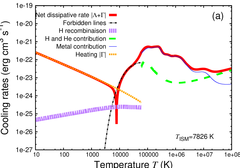
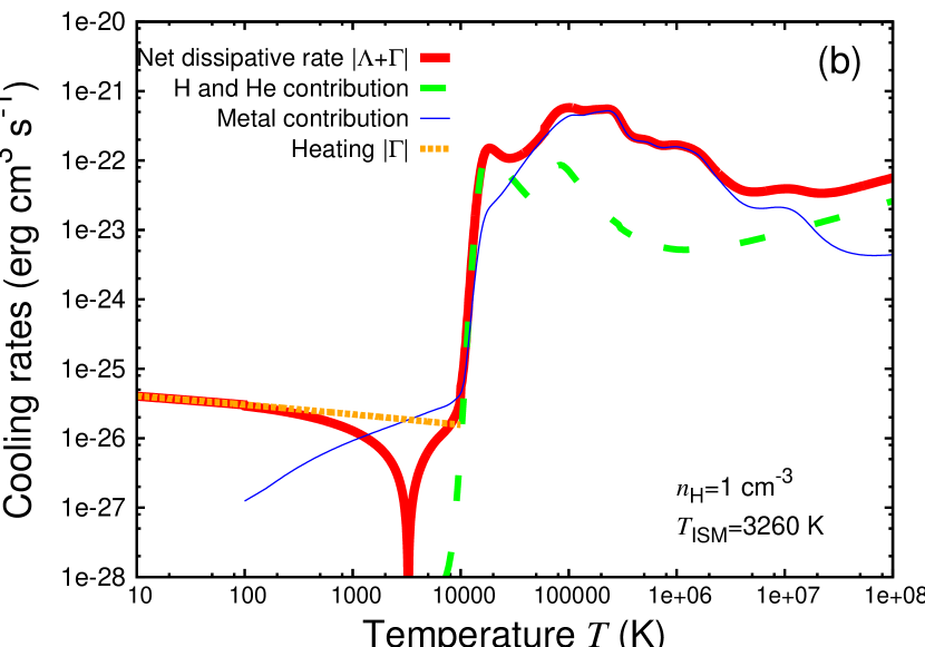
Figure 4: Cooling and heating rates as a function of temperature for photoionized (a) and collisional ionization equilibrium (b) medium. The solid thick red line is the curve representing the net rate of emitted energy, i.e. the absolute value of the sum of the luminosity due to cooling $\it\Lambda$ and heating $\it\Gamma$. Dotted and thin lines correspond to the different processes the model takes into account: emission from forbidden lines (dotted dashed thin black), H recombination lines (dotted thick purple), hydrogen and helium (dashed green) and metals (solid thin blue) as well as the heating rate $\it\Gamma$ (dotted orange). All luminosity from the different coolants and heating rate of processes are presented for $n_{\rm H}=1\,\rm cm^{-3}$, within their range of interest. The $x$-axis represents temperature (in $\mathrm{K}$) and the $y$-axis the emitted energy (in $\rm erg\,s^{-1}\,\rm cm^{3}$).

At low temperatures ($T<6\times 10^{4}\,\mathrm{K}$), the cooling rate is the sum of all terms $\it\Lambda_{\mathrm{H+He}}$, $\it\Lambda_{\mathrm{Z}}$, $\it\Lambda_{\mathrm{RR}}$ and $\it\Lambda_{\mathrm{FL}}$, whereas for higher temperatures ($T>6\times 10^{4}\,\mathrm{K}$) only the ones for hydrogen, helium and $Z$ are used. The two parts of the curve are linearly interpolated in the range of $4.5\times 10^{4}<T<6.0\times 10^{4}\,\mathrm{K}$.

The CIE cooling curve (see panel (b) of Fig. 4) also assumes solar abundances (Wiersma et al., 2009) for hydrogen, helium and $Z$. The heating term $\mathit{\Gamma}_{1}$ represents the photoelectric heating of dust grains by the Galactic far-UV background. For $T\leq 1000\,\mathrm{K}$, we used equation  C5 of Wolfire et al. (2003). We impose a low temperature ($T<1000\,\mathrm{K}$) electron number density profile $n_{\rm e}$ using eq. C3 of Wolfire et al. (2003). For $T>1000\,\mathrm{K}$ we take the value of $n_{\rm e}$ interpolated from the CIE curve by Wiersma et al. (2009).

A transition between the main sequence and the red supergiant phases requires a transition between photoionized and CIE medium. At the beginning of the red supergiant phase, our model ceases to consider the dissipation and heating for photoionized medium and adopts the ones assuming CIE medium. The assumption of CIE specifies $n_{\mathrm{e}}/n_{\mathrm{H}}$ as a function of $T$ (Wiersma et al., 2009). The mean mass per particle is calculated as,

$$\mu(T)=\frac{1+4\mathit{\chi}_{\mathrm{He}}}{(1+\mathit{\chi}_{\mathrm{He}})[1+x(T)]},$$ (11)

where,

$$x(T)=\Big{(}\frac{n_{\mathrm{e}}}{n_{\mathrm{H}}}\Big{)}_{T}/\Big{(}\frac{n_{\mathrm{e}}}{n_{\mathrm{H}}}\Big{)}_{T_{\mathrm{max}}},$$ (12)

and $T_{\rm max}$ is the upper limit of the cooling curve temperature range (Wiersma et al., 2009), and $x(T)$ is a quantity monotonically increasing with $T$, that gives the degree of ionization of the medium (see top inset in Fig. 5). We then have an expression for $\mu$ with low and high $T$ limits of $\mu=1.27$ and $\mu=0.61$ for neutral and fully ionized medium, respectively (e.g. Lequeux, 2005). For simulations assuming CIE we then obtain through $\mu(T)$ a one-to-one correspondence between $T/\mu\propto p/\rho$ (known) and $T$ (required) for each cell of the computational domain.

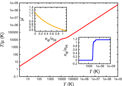
Figure 5: Temperature divided by the mean mass per particle $T/\mu$ (in $\mathrm{K}$) as a function of temperature $T$ (in $\mathrm{K}$). Data are derived from the collisional ionization equilibrium cooling curves (Wiersma et al., 2009). Top inset: $\mu$ as a function of electron fraction $n_{\mathrm{e}}/n_{\mathrm{H}}$. Bottom inset: $n_{\mathrm{e}}/n_{\mathrm{H}}$ as a function of temperature $T$.

2.5 Thermal conduction

The circumstellar medium around runaway main sequence stars presents large temperature gradients across its shocks and discontinuities (e.g. $\mathit{\Delta}T\approx 10^{7}\,\rm K$ at the reverse shock of the models for the $20$ and $40\,M_{\odot}$ stars), which drive the heat flux (Spitzer, 1962; Cowie & McKee, 1977). Electrons move quickly enough to transfer energy to the adjacent low temperature gas. The consequent equilibration of the pressure smooths the density profiles at the discontinuity between the wind and ISM material (Weaver et al., 1977).

Heat conduction is included in our models over the whole computational domain. For the models with partially neutral gas, e.g. during a phase transition or for models involving a red supergiant, $\mn@boldsymbol{F}_{\rm c}$ is calculated at $T<1000\,\rm K$ with $n_{\rm e}$ from eq. C3 in Wolfire et al. (2003). Our study does not consider either the stellar or interstellar magnetic field, which make the heat conduction anisotropic (Orlando et al., 2008).

2.6 Relevant characteristic quantities of a stellar wind bow shock

A stellar wind bow shock generally has four distinct regions: the unperturbed ISM, the shocked ISM, the shocked wind material and the freely-expanding wind. The shocked materials are separated by a contact discontinuity, the expanding wind from the star is separated from shocked wind by the reverse shock and the structure’s outermost border is marked by the forward shock (e.g. van Buren, 1993).

The stand-off distance of the bow shock is,

$$R(0)=\sqrt{\frac{\dot{M}v_{\mathrm{w}}}{4\pi\rho_{\mathrm{ISM}}v_{\star}^{2}}}$$ (13)

(Baranov et al., 1971). The analytical approximation for the shape of an infinitely thin bow shock is,

$$R({\theta})=R(0)\mathrm{cosec}(\theta\frac{\pi}{180})\sqrt{3(1-\theta\frac{\pi}{180})\mathrm{cotan}(\theta\frac{\pi}{180})},$$ (14)

where $\theta$ is the angle from the direction of motion in degrees and $R(0)$ is given by Eq. (13).

The dynamical timescale of a layer constituting a stellar wind bow shock is equal to the time a fluid element spends in it before it is advected downstream,

$$t_{\mathrm{dyn}}=\frac{\Delta z}{v},$$ (15)

where $\Delta z$ is the thickness of the layer along the $Oz$ direction and $v$ is a characteristic velocity of the gas in the considered region, i.e. the post-shock velocity $v\simeq v_{\rm w}/4$ in the shocked wind or $v\simeq v_{\star}/4$ in the shocked ISM. The gas density and pressure govern the cooling timescale,

$$t_{\mathrm{cool}}=\frac{E}{\dot{E}}=\frac{p}{(\gamma-1)\mathit{\Lambda}(T)n_{\rm H}^{2}}.$$ (16)

These two timescales determine whether a shock is adiabatic ($t_{\mathrm{dyn}}\ll t_{\mathrm{cool}}$) or radiative ($t_{\mathrm{dyn}}\gg t_{\mathrm{cool}}$).

2.7 Presentation of the simulations

The parameters used in our simulations are gathered together with information concerning the size of the computational domain in Table 1. The size of the computational domain is inspired by Comerón & Kaper (1998), i.e. we use a sufficient number of cells $N_{\rm R}$ to adequately resolve the substructures of each bow shock in the direction of the stellar motion. As $v_{\star}$ increases, the bow shock and the domain size decreases, so the spatial resolution $\it\Delta=R_{\rm max}/N_{\rm R}$ also decreases. The dimensions of the domain are chosen such that the tail of the bow shock only crosses the $\it z=\it z_{\rm min}$ boundary, but never intercepts the outer radial border at $\it R=\it R_{\rm max}$ to avoid numerical boundary effects.

We model bow shocks for a space velocity $20\,\leq v_{\star}\leq 70\,\rm km\,\rm s^{-1}$, since these include the most probable space velocities of runaway stars and ranges from supersonic to hypersonic (Eldridge et al., 2011). For the bow shocks of main sequence stars the label is MS, and the models for the red supergiant phase are labelled with the prefix RSG. In our nomenclature, the four digits following the prefix of a model indicate the zero age main sequence mass (first two digits) and the space velocity (next two digits).

Simulations of bow shocks involving a main sequence star are started at a time $t_{\rm start}$ in the middle of their stellar evolutionary phase in order to model bow shocks with roughly constant wind properties. The distortion of the initially spherically expanding bubble into a steady bow shock takes up to $\approx 16\,t_{\rm cross}$, where $t_{\rm cross}=R(0)/v_{\star}$ is the bow shock crossing-time. We stop the simulations at least $32\,t_{\rm cross}$ after the beginning of the integration, except for model MS4020 for which such a time is larger than the main sequence time.

Table 1: Nomenclature and grid parameters used in our hydrodynamical simulations. Parameters $\it\Delta$, $R_{\mathrm{max}}$ and $z_{\mathrm{min}}$ are the resolution of the uniform grid (in $\mathrm{pc}\,\mathrm{{cell}^{-1}}$) and respectively the upper and lower limits of the domain along the $x$-axis and $y$-axis (in $\mathrm{pc}$). $N_{\mathrm{R}}$ and $N_{\mathrm{z}}$ are the number of cells discretising the corresponding directions. The two last columns contain the starting time $t_{\mathrm{start}}$ of the simulations relative to the zero-age main-sequence and the crossing time $\,t_{\rm cross}$ of the gas because of the stellar motion for each associated bow shock (in $\mathrm{Myr}$).

${\rm{Model}}$	$M_{\star}\,(M_{\odot})$	$v_{\star}\,(\mathrm{km}\,\mathrm{s}^{-1})$	$\mathit{\Delta}\,(\mathrm{pc}\,\mathrm{cell}^{-1})$	$z_{\mathrm{min}}\,(\mathrm{pc})$	$R_{\mathrm{max}}\,(\mathrm{pc})$	$N_{\rm R}$	$N_{\rm z}$	$t_{\mathrm{start}}\,(\mathrm{Myr})$	$t_{\mathrm{cross}}\,(\mathrm{Myr})$
MS1020	$10$	$20$	$1.7\times 10^{-3}$	$-0.5$	$1.0$	$600$	$600$	$5.0$	$6.3\times 10^{-2}$
MS1040	$10$	$40$	$5.7\times 10^{-4}$	$-0.2$	$0.4$	$700$	$700$	$5.0$	$1.6\times 10^{-3}$
MS1070	$10$	$70$	$3.3\times 10^{-4}$	$-0.1$	$0.2$	$600$	$600$	$5.0$	$4.9\times 10^{-4}$
RSG1020	$10$	$20$	$8.0\times 10^{-3}$	$-2.00$	$4.0$	$500$	$500$	$22.62$	$1.5\times 10^{-2}$
RSG1040	$10$	$40$	$2.3\times 10^{-3}$	$-0.7$	$1.4$	$600$	$600$	$22.78$	$5.5\times 10^{-3}$
RSG1070	$10$	$70$	$7.5\times 10^{-4}$	$-0.3$	$0.6$	$800$	$800$	$22.86$	$2.1\times 10^{-3}$
MS2020	$20$	$20$	$2.0\times 10^{-2}$	$-5.0$	$10.0$	$500$	$500$	$3.0$	$7.0\times 10^{-2}$
MS2040	$20$	$40$	$8.3\times 10^{-3}$	$-2.5$	$5.0$	$600$	$600$	$3.0$	$1.7\times 10^{-2}$
MS2070	$20$	$70$	$2.1\times 10^{-3}$	$-0.75$	$1.5$	$700$	$700$	$3.0$	$5.4\times 10^{-3}$
RSG2020	$20$	$20$	$1.0\times 10^{-2}$	$-5.0$	$15.0$	$1000$	$1500$	$8.0$	$6.8\times 10^{-2}$
RSG2040	$20$	$40$	$7.5\times 10^{-3}$	$-3.0$	$6.0$	$800$	$800$	$8.0$	$1.6\times 10^{-2}$
RSG2070	$20$	$70$	$6.7\times 10^{-3}$	$-2.0$	$4.0$	$600$	$600$	$8.0$	$4.4\times 10^{-3}$
MS4020	$40$	$20$	$6.0\times 10^{-2}$	$-15.0$	$30.0$	$500$	$500$	$0.0$	$2.8\times 10^{-1}$
MS4040	$40$	$40$	$2.7\times 10^{-2}$	$-8.0$	$16.0$	$600$	$600$	$0.0$	$7.1\times 10^{-2}$
MS4070	$40$	$70$	$1.1\times 10^{-2}$	$-4.0$	$8.0$	$700$	$700$	$0.0$	$2.5\times 10^{-2}$

3 The main sequence phase

3.1 Physical characteristics of the bow shocks

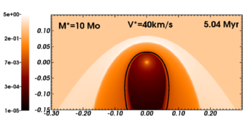
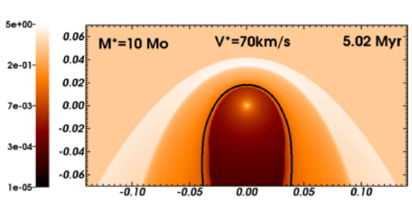
Figure 6: Grid of stellar wind bow shocks from the main sequence phase of the $10\,M_{\odot}$ initial mass star as a function of the space velocity with respect to the ISM, with $20\,\mathrm{km}\,\mathrm{s}^{-1}$ (top panel), $40\,\mathrm{km}\,\mathrm{s}^{-1}$ (middle panel) and $70\,\mathrm{km}\,\mathrm{s}^{-1}$ (bottom panel). The nomenclature of the models follows Table 1. The gas number density is shown with a density range from $10^{-5}$ to $5.0\,\mathrm{cm}^{-3}$ in the logarithmic scale. The solid black contour traces the boundary between wind and ISM material $Q(\mn@boldsymbol{r})=1/2$. The $x$-axis represents the radial direction and the $y$-axis the direction of stellar motion (in $\mathrm{pc}$). Only part of the computational domain is shown.

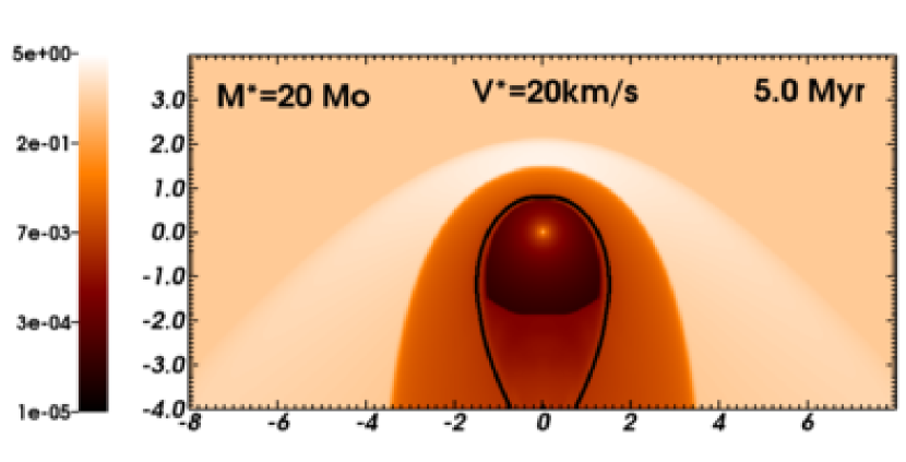
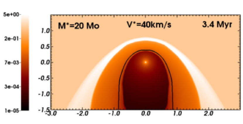
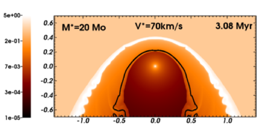
Figure 7: As Fig. 6, with an initial stellar mass of $20\,M_{\odot}$.

We show the gas density field in our bow shock models of the main sequence phase MS1020 ($10\,M_{\odot}$ initial stellar mass, $v_{\star}=20\,\mathrm{km}\,\mathrm{s}^{-1}$, upper panel), MS1040 ($10\,M_{\odot}$, $40\,\mathrm{km}\,\mathrm{s}^{-1}$, middle panel) and MS1070 ($10\,M_{\odot}$, $70\,\mathrm{km}\,\mathrm{s}^{-1}$, lower panel) in Fig. 6. Figs. 7 and 8 are similar for the $20\,M_{\odot}$ and $40\,M_{\odot}$ initial mass stars. The figures correspond to a time $\approx t_{\rm start}+32\,t_{\rm cross}$. The model MS4020 has a lifetime $<32\,t_{\rm cross}$ (see panels (c) and (f) of Fig. 3), and is therefore shown at a time $\approx 16\,t_{\rm cross}$. In Figs. 6 to 8 the overplotted solid black line is the material discontinuity, i.e. the border between the wind and ISM gas where the value of the material tracer $Q(\mn@boldsymbol{r})=1/2$. The bow shock morphological characteristics such as the stand-off distance and the axis ratio $R(0)/R(90)$ measured from the simulations are summarised in Table 2.

The theory of Baranov et al. (1971) predicts that $R(0)\propto v_{\star}^{-1}$ and $R(0)\propto\dot{M}^{1/2}$ because the stand-off distance depends on the balance between the wind ram pressure with the ISM ram pressure. The size of the bow shock decreases as a function of $v_{\star}$: $R(0)$ decreases by a factor of 2 if $v_{\star}$ doubles, e.g. $R(0)\approx 0.13$ in model MS1020 but $R(0)\approx 0.06$ in model MS1040 (see upper and middle panels of Fig. 6). The bow shocks also scale in size with $\dot{M}$, e.g. at fixed $v_{\star}$ its size for the $10\,M_{\odot}$ star is smaller by a factor of 10 compared to the size of the bow shock from the $20\,M_{\odot}$ star, which in turn is smaller by a factor of $\approx 3.5$ compared to one from the $40\,M_{\odot}$ star (e.g. see middle panels of Figs. 6 to 8). If we look again at $\dot{M}$ in Fig. 3 (a$-$c), we find $\dot{M}\approx 10^{-9.5}$, $\approx 10^{-7.3}$ and $\approx 10^{-6}\,\rm M_{\odot}\,\rm yr^{-1}$ for the $10$, $20$ and $40\,M_{\odot}$ star, respectively. We see that these sizes are in accordance with the theory and arise directly as a result of Eq. (13).

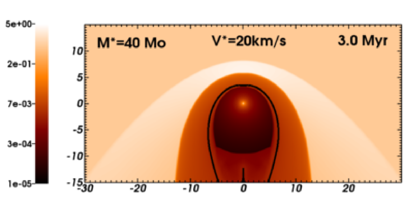
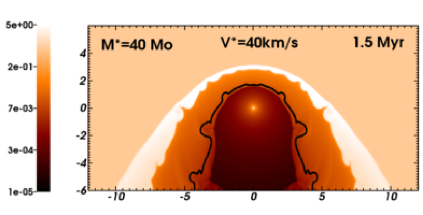
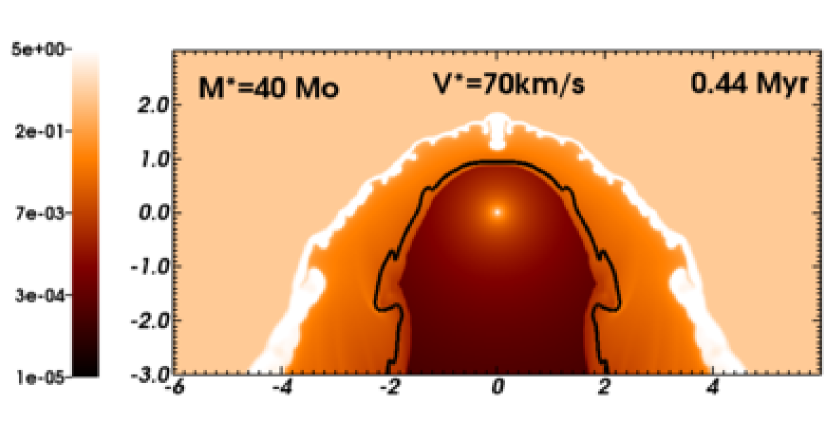
Figure 8: As Fig. 6, with an initial stellar mass of $40\,M_{\odot}$.

The relative thickness of the substructures varies with the wind and ISM properties because the gas velocity determines both the post-shock temperature, i.e. governs the cooling physics at the reverse shock and in the shell, and the compression of the shocked ISM. Our simulations with $v_{\star}=20\,\mathrm{km}\,\mathrm{s}^{-1}$ have weak forward shocks, i.e. compression at the forward shock is not important. The thickness of the layer of shocked ISM gas with respect to $R(0)$ is roughly independent of $M_{\star}$ for these models (see upper panels of Figs. 6, 7 and 8). The shocked ISM density increases for models with $v_{\star}\geq 40\,\mathrm{km}\,\mathrm{s}^{-1}$ because the high post-shock temperature makes the cooling efficient. The variations of $\dot{M}$ at a given $v_{\star}$ modify the morphology of the bow shock because a stronger wind ram pressure enlarges the size of the bow shock and makes the shell thinner with regard to $R(0)$ (see models MS1020 and MS4020 in upper panels of Figs. 6 and 8).

Our simulations with $v_{\star}=20\,\mathrm{km}\,\mathrm{s}^{-1}$ all have a stable density field (see upper panels of Figs. 6 to 8). The simulations with $v_{\star}=40\,\mathrm{km}\,\mathrm{s}^{-1}$ are bow shocks with radiative forward shocks (i.e. with a dense and thin layer of shocked ISM). Our simulations for $M_{\star}\geq 20\,M_{\odot}$ and with $v_{\star}=70\,\rm km\,\rm s^{-1}$ show instabilities at both the contact and the material discontinuity, see middle panel of Fig. 7 and 8. Our models for the $40\,M_{\odot}$ star with $v_{\star}\geq 40\,\rm km\,\rm s^{-1}$ are similar. Model MS4040 is slightly more unstable than model MS2070 whereas model MS4070 shows even stronger instability which develops at its forward shock and dramatically distorts its dense and thin shell, as shown in the bottom panel of Fig. 8. The large density gradient across the material discontinuity allows Rayleigh-Taylor instabilities to develop. The entire shell of cold ISM gas has distortions characteristic of the non-linear thin-shell instability (Vishniac, 1994; Garcia-Segura et al., 1996).

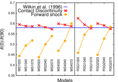
Figure 9: Comparison between the ratio $R(0)/\mathrm{R}(90)$ for the main sequence and supergiant models with the theoretical value of $1/\sqrt{3}\approx 0.58$ predicted by Wilkin (1996, horizontal dotted blue line). We distinguish between the contact discontinuity (red crosses) and the forward shock (orange dots) of each model.

3.2 Comparison of the models with the analytical solution

In Fig. 9 we compare $R(0)/R(90)$ with the analytical solution for a bow shock with a thin shell ($R(0)/R(90)\approx 1/\sqrt{3}\approx 0.58$; Wilkin, 1996). $R(0)/R(90)$ at the contact discontinuity decreases as a function of $v_{\star}$, e.g. models MS2020 and MS2070 have $R(0)/R(90)\approx 0.59$ and $\approx 0.56$, respectively. $R(0)/R(90)$ at the forward shock increases with $v_{\star}$ and $\dot{M}$ (see Figs. 6 to 8). The contact discontinuity is the appropriate measure to match the analytical solution (see Mohamed et al., 2012). $R(0)/R(90)$ is within $<10$ per cent of Wilkin’s solution but does not satisfy it at both discontinuities, except for MS4070 with $R(0)/R(90)\approx 0.59$ at the contact discontinuity and $R(0)/R(90)\approx 0.60$ at the forward shock. Model MS4070 is the most compressive bow shock and it has a thin unstable shell bounded by the contact discontinuity and forward shock. Fig. 10 shows good agreement between model MS4070 and Wilkin’s solution for angles $\theta>90^{\circ}$. Our model MS4020 is the most deviating simulation at the forward shock, because the brevizy of its main sequence phase prevents the bow shock from reaching a steady state.

Figure 10: Comparison between the density field of model MS4070 presenting a thin shell and the corresponding analytical solution (Wilkin, 1996, solid black line). The gas number density is shown with a density range from $10^{-5}$ to $5.0\,\rm cm^{-3}$ in the logarithmic scale. The $x$-axis represents the radial direction and the $y$-axis the direction of stellar motion (in $\mathrm{pc}$).

Table 2: Bow shock morphological properties at the contact discontinuity. The parameter $R(0)$ (in pc) is the stand-off distance of the bow shock at the contact discontinuity and $R(0)/R(90)$ is the ratio plotted in Fig. 9, with $R(90)$ the radius perpendicular to the direction of motion.

${\rm{Model}}$	$R(0)\,(\rm pc)$	$R(0)/R(90)$
MS1020	$0.13$	$0.595$
MS1040	$0.06$	$0.587$
MS1070	$0.03$	$0.586$
RSG1020	$0.30$	$0.625$
RSG1040	$0.22$	$0.594$
RSG1070	$0.15$	$0.576$
MS2020	$1.40$	$0.590$
MS2040	$0.69$	$0.582$
MS2070	$0.38$	$0.563$
RSG2020	$1.35$	$0.600$
RSG2040	$0.65$	$0.590$
RSG2070	$0.31$	$0.578$
MS4020	$5.60$	$0.598$
MS4040	$2.85$	$0.593$
MS4070	$1.72$	$0.587$

3.3 Thermal conduction

Fig. 11 illustrates the effects of heat conduction on the shape of a bow shock. Panel (a) shows the density field of model MS2040, and panel (b) shows the same model but without thermal conduction. The dashed contour traces the border between wind and ISM gas. The streamlines show the penetration of ISM material into the hot bubble. The bow shock including thermal conduction is larger by a factor $\approx 1.4$ in both the directions normal and parallel to the direction of motion of the star. Its shell is denser and splits into two layers of hot and cold shocked ISM, whereas the model without thermal conduction has a single and less compressed region of ISM material.

The position of the reverse shock is insensitive to thermal conduction because heat lost at the material discontinuity is counterbalanced by the large wind ram pressure (see panels (a) and (b) of Fig. 11). Fig. 12 illustrates that the shocked regions of a bow shock with heat conduction have smooth density profiles around the contact discontinuity (see panels (a) and (c) of Fig. 12). This is consistent with previous models of a steady star (see fig. 3 of Weaver et al., 1977) and of moving stars (see Fig. 7 of Comerón & Kaper, 1998). Electrons carry internal energy from the hot shocked wind to the shocked ISM, e.g. the $10\,M_{\odot}$ models have a temperature jump amplitude of $\mathit{\Delta}T\approx 10^{7}\,\rm K$ across the contact discontinuity.

Our simulation of model MS1040 (see Fig. 6) provides us with the parameters of the hot bubble ($T\approx 10^{7}\,\rm K$, $n\approx 0.02\,\rm cm^{-3}$) and the shell ($T\approx 10^{4}\,\rm K$, $n\approx 3.3\,\rm cm^{-3}$). The shocked ISM gas has a velocity $v\approx 25\,\rm km\,\rm s^{-1}$ and $\mu=0.61$. Using Eq. (15)$-$(16), we find that the hot gas in the inner ($t_{\rm cool}\approx 1.11\times 10^{2}\gg t_{\rm dyn}\approx 1.4\times 10^{-3}\,\rm Myr$ ) and outer ($t_{\rm cool}\approx 2.94\times 10^{-3}\gtrsim t_{\rm dyn}\approx 1.0\times 10^{-3}\,\rm Myr$ ) layers of the bow shock are adiabatic and slightly radiative, respectively. The radiative character of the shell is more pronounced for models with $v_{\star}>40\,\rm km\,\rm s^{-1}$. Note that the hot bubble never cools, i.e. $t_{\rm cool}$ refers here to the timescale of the losses of internal energy by optically-thin radiative processes, which are compensated by the conversion of kinetic energy to heat at the reverse shock. The thermal conduction timescale is,

$$t_{\rm cond}=\frac{7pl^{2}}{2(\gamma-1)\kappa(T)T},$$ (17)

where $\kappa(T)$ is the heat conduction coefficient and $l$ a characteristic length along which heat transfer happens (Orlando et al., 2008). Because $\kappa(T)\propto T^{5/2}$ (Cowie & McKee, 1977), $t_{\rm cond}\propto T^{-7/2}$, i.e. heat conduction is a fast process in a hot medium. Consequently, we have $t_{\rm dyn}/t_{\rm cond}\approx 1.46\times 10^{5}\gg 1$ and $t_{\rm cool}/t_{\rm cond}\approx 1.16\times 10^{10}\gg 1$ in the hot bubble ($l=0.035\,\rm pc$) whereas we find $t_{\rm dyn}/t_{\rm cond}\approx 1.71\times 10^{-5}\ll 1$ and $t_{\rm cool}/t_{\rm cond}\approx 5.03\times 10^{-5}\ll 1$ in the shell ($l=0.025\,\rm pc$) of the model MS1040, which explains the differences between the models shown in Fig. 11. All of our simulations of the main sequence phase behave similarly because their hot shocked wind layers have similar temperatures. Heat transfer across the bubble is always faster than the dynamical timescale of the gas.

As a consequence, the pressure increases in the shocked ISM, pushing both the contact discontinuity inwards and the forward shock outwards. The region of shocked wind conserves its mass but loses much of its pressure. To balance the external pressure, its volume decreases and the gas becomes denser. Two concentric substructures of shocked ISM form: an inner one with high temperature and low density adjoining the material discontinuity, and an outer one with low temperature and high density. Previous investigations about the effects of heat conduction inside circumstellar nebulae around runaway hot stars are available in section 4.6 of Comerón & Kaper (1998).

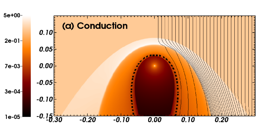
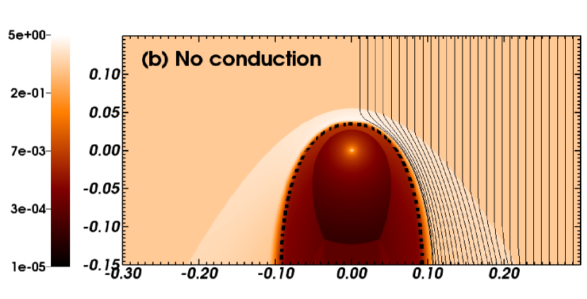
Figure 11: Changes in the location of ISM and wind material induced by thermal conduction in the hot bubble of a bow shock. Figures show gas number density (in $\rm cm^{-3}$) for model $\mathrm{MS1040}$ (a) and for the same setup run without heat conduction (b). For each figure the dotted thick line traces the material discontinuity, $Q(\mn@boldsymbol{r})=1/2$. The right part of each figure overplots ISM flow streamlines. It highlights the penetration of ISM material into the hot layer of the bow shock because of heat conduction. Comparing the two figures illustrates its effects, increasing the density inside the region of shocked wind and enlarging the global size of the bow shock. The $x$-axis represents the radial direction and the $y$-axis the direction of stellar motion (in $\mathrm{pc}$). Only part of the computational domain is shown.

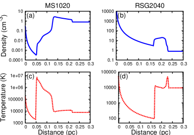
Figure 12: Total number density (solid blue lines, in $\mathrm{cm}^{-3}$) and temperature (dotted red lines, in $\mathrm{K}$) profiles for two typical bow shocks of a main sequence and a red supergiant star. The profiles are plotted for the model MS1020 in panels (a) and (c) and for the model RSG2040 in panels (b) and (d) as a function of the distance to the star along the direction of motion.

3.4 Bow shock emissivity

3.4.1 Luminosities

The bow shock luminosities of all our models are plotted in panel (a) of Fig. 13. It shows the emitted light as a function of mass-loss $\dot{M}$ and space velocity $v_{\star}$ (i.e. by model). $L_{\rm gas}$ is the bow shock luminosity from optically-thin cooling of the gas and the part of this which originates from the wind material is designated as $L_{\rm wind}$. The bow shock luminosities are calculated taking into account the cylindrical symmetry of the models by integrating the radiated energy in the $z\geq 0$ region (Mohamed et al., 2012). The optically-thin gas radiation is therefore computed as,

$$\mathit{L}_{\rm gas}=2\pi\iint_{\mathcal{D}}\mathit{\Lambda}n_{\rm H}^{2}RdRdz,$$ (18)

where $\mathcal{D}$ represents the considered volume. The heating terms are estimated with a similar method, as,

$$\widetilde{\mathit{\Gamma}}_{\alpha}=2\pi\iint_{\mathcal{D}}\mathit{\Gamma}_{\alpha}n_{\rm H}^{\alpha}RdRdz,$$ (19)

where $\widetilde{\mathit{\Gamma}}_{\alpha=1}$ is the heating rate per unit volume for UV heating of grains, and $\widetilde{\mathit{\Gamma}}_{\alpha=2}$ is the heating rate per unit volume square for photoionization heating. Inserting the quantities $Q(\mn@boldsymbol{r})$ or $1$$-$$Q(\mn@boldsymbol{r})$ in the integrant of Eq. (18) or (19) allows us to separate the contributions from wind and ISM material. The panels of Fig. 13 also specify the luminosity from H${\alpha}$ emission $L_{\rm H\alpha}$ (calculated using the prescriptions by Osterbrock & Bochkarev (1989), our Appendix A) and the infrared luminosity of reprocessed starlight by dust grains $L_{\rm IR}$ (calculated treating the dust as in Mackey et al. (2012), our Appendix B). Nonetheless, $L_{\rm IR}$ does not contribute to the thermal physics of the plasma and is not included in the calculations of either $L_{\rm gas}$ or $L_{\rm wind}$. The luminosities $L_{\rm gas}$, $L_{\rm wind}$, $L_{\rm H\alpha}$, $L_{\rm IR}$, the heating rates $\widetilde{\mathit{\Gamma}}_{\alpha}$, and the stellar luminosity $L_{\star}$, provided by the stellar evolution models (Brott et al., 2011), are detailed in Table 3.

The bow shock luminosity of optically thin gas $L_{\rm gas}$ decreases by an order of magnitude between the models with $v_{\star}=20$ to $70\,\rm km\,s^{-1}$, but increases by several orders of magnitude with $\dot{M}$, e.g. $L_{\rm gas}\approx 1.4\times 10^{31}$ and $\approx 3.9\times 10^{35}\,\rm erg\,\rm s^{-1}$ for the models MS1020 and MS4020, respectively. $L_{\rm gas}$ is influenced by i) $v_{\star}$ which governs the compression factor of the shell, and ii) by the size of the bow shock which increases with $\dot{M}$ and decreases with $v_{\star}$. Moreover, we find that emission by optically-thin cooling is principally caused by optical forbidden lines such as [O ii] and [O iii] which is included in the cooling curve in the range $\approx 8000\leq T\leq 6.0\times 10^{4}\,\rm K$ (see estimate of the luminosity $L_{\rm FL}$ produced by optical forbidden lines in Table 3).

The contribution of optically-thin emission from stellar wind material, $L_{\rm wind}$, to the total luminosity of optically-thin gas radiation is negligible e.g. $L_{\rm wind}/L_{\rm gas}\approx 10^{-6}$ for model MS2020. The variations of $L_{\rm wind}$ roughly follows the variations of $L_{\rm gas}$. The volume occupied by the shocked wind material is reduced by heat transfer (see black contours in Figs. 6 to 8) and this prevents $L_{\rm wind}$ from becoming important relative to $L_{\rm gas}$. It implies that most of the emission by radiative cooling comes from shocked ISM gas which cools as the gas is advected from the forward shock to the contact discontinuity.

$L_{\rm H\alpha}$ is smaller than $L_{\rm gas}$ by about $1$$-$$3$ orders of magnitude and larger than $L_{\rm wind}$ by $2$$-$$5$ orders of magnitude, e.g. model MS2040 has $L_{\rm H\alpha}/L_{\rm gas}\approx 10^{-1}$ and $L_{\rm H\alpha}/L_{\rm wind}\approx 10^{4}$. The H$\alpha$ emission therefore mainly comes from ISM material. More precisely, we suggest that $L_{\rm H\alpha}$ originates from the cold innermost shocked ISM since the H$\alpha$ emissivity $\propto T^{-0.9}$ (our Appendix A). The variations of $L_{\rm H\alpha}$ follow the global variations of $L_{\rm gas}$, i.e. the H$\alpha$ emission is fainter at high $v_{\star}$, e.g. $L_{\rm H\alpha}\approx 1.3\times 10^{33}$ and $\approx 3.6\times 10^{31}\,\mathrm{erg}\,\mathrm{s}^{-1}$ for models MS2020 and MS2070, respectively. The gap between $L_{\rm gas}$ and $L_{\rm H\alpha}$ increases with $v_{\star}$ because the luminosities are calculated for $z>0$ whereas the H$\alpha$ maximum is displaced to $z<0$ as $v_{\star}$ increases (see further discussion in Section 3.4.2).

$L_{\rm IR}$ is larger than $L_{\rm gas}$ by about $1$$-$$3$ orders of magnitude in all our simulations. We find that $L_{\rm IR}\gg L_{\rm H\alpha}$, with a gap increasing with $v_{\star}$ at a considered $\dot{M}$, e.g. $L_{\rm IR}/L_{\rm H\alpha}\approx 10^{2}$ and $\approx 10^{3}$ for models MS2020 and MS2070, respectively. These large $L_{\rm IR}$ suggest that bow shocks around main sequence stars should be much more easily observed in the infrared than at optical wavelength. We draw further conclusions on the detectability of bow shocks generated by a runaway main sequence stars moving through the Galactic plane in Section 6.2.

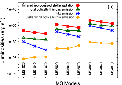
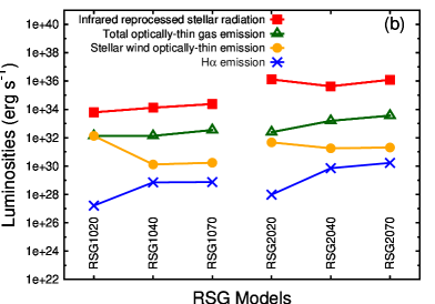
Figure 13: Bow shock luminosities and reprocessed stellar infrared radiation for main sequence (a) and red supergiant models (b). The total bow shock luminosity of optically-thin gas radiation (green triangles) is distinguished from the contribution due to the wind material only (orange dots). The luminosity of H$\alpha$ emission (blue crosses) and the reprocessed infrared stellar radiation (red squares) are also plotted. The infrared radiation is not considered in the simulations and is therefore not included in the total optically-thin gas radiation. The simulation labels are written vertically under each triplet related to a given stellar model (see Table 1).

3.4.2 Synthetic emission maps

Figs. 14, 15 and 16 show synthetic H$\alpha$ emission maps of the bow shocks (left) together with dust surface mass density maps (right), from the slowest ($v_{\star}=20\,\rm km\,\rm s^{-1}$, top panels) to the highest ($v_{\star}=70\,\rm km\,\rm s^{-1}$, bottom panels) models, respectively. These maps take into account the rotational symmetry of the coordinate system (our Appendix A). The ISM background is ignored, i.e. we set its density to zero in the computation of the projected emissivity and dust density, so that the surface brightness and the surface mass density only refer to the bow shocks. The dust surface density is calculated by projecting the shocked ISM gas weighted by a gas-to-dust ratio (our Appendix B), i.e. we considered that the wind material of a star is dust free during the main sequence.

The region of maximum H$\alpha$ surface brightness is located at the apex of the bow shocks in the simulations with $v_{\star}=20\,\rm km\,\rm s^{-1}$ and extends or displaces to its tail (i.e. $z<0$) as $v_{\star}$ increases. As the ISM gas enters a bow shock generated by a main sequence star, its density increases and the material is heated by thermal conduction towards the contact discontinuity, so its H$\alpha$ emissivity decreases (see panels (a) and (c) of Fig. 12). The competition between temperature increase and gas compression produces the maximum emission at the contact discontinuity which separates hot and cold shocked ISM gas. The reverse shock and the hot bubble are not seen because of both their low density and their high post-shock temperature. Simulations with $v_{\star}\geq 40\,\rm km\,\rm s^{-1}$ have their peak emissivity in the tail of the bow shock because the gas does not have time to cool at the apex before it is advected downstream. Simulations with high $v_{\star}$ and strong $\dot{M}$ (e.g. model MS4070) have bow shocks shining in H$\alpha$ all along their contact discontinuity, i.e. the behaviour of the H$\alpha$ emissivity with respect to the large compression factor in the shell ($\propto n^{2}$) overwhelms that of the post-shock temperature ($\propto T^{-0.9}$).

The dust surface mass density increases towards the contact discontinuity (see left panels of Figs. 14 to 16). Panel (a) of Fig. 17 shows that normalized cross-sections of both the H$\alpha$ surface brightness and the dust surface mass density of model MS2040, taken along the direction of motion of the star in the $z\geq 0$ region of the bow shock, peak at the same distance from the star. We find a similar behaviour for all our bow shock models of hot stars. This suggests that both maximum H$\alpha$ and infrared emission originate from the same region, i.e. near the contact discontinuity in the cold region of shocked ISM material constituting the outermost part of a bow shock generated by a main sequence star.

The maximum H$\alpha$ surface brightness of the brightest models (e.g. model MS2020) is $\geq 6\times 10^{-17}\,\mathrm{erg}\,\mathrm{s}^{-1}\,\mathrm{cm}^{-2}\,\mathrm{arcsec}^{-2}$, which is above the diffuse emission sensitivity limit of the SuperCOSMOS H-alpha Survey (SHS; Parker et al. 2005) of $1.1$$-$$2.8\times 10^{-17}\,\mathrm{erg}\,\mathrm{s}^{-1}\,\mathrm{cm}^{-2}\,\mathrm{arcsec}^{-2}$ and could therefore be observed. The bow shocks around a central star less massive than $20\,M_{\odot}$ are fainter and could be screened by the $\rm{H}\,{\textsc{ii}}$ region generated by their driving star. This could explain why we do not see many stellar wind bow shocks around massive stars in H$\alpha$.

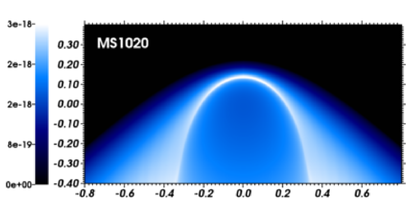
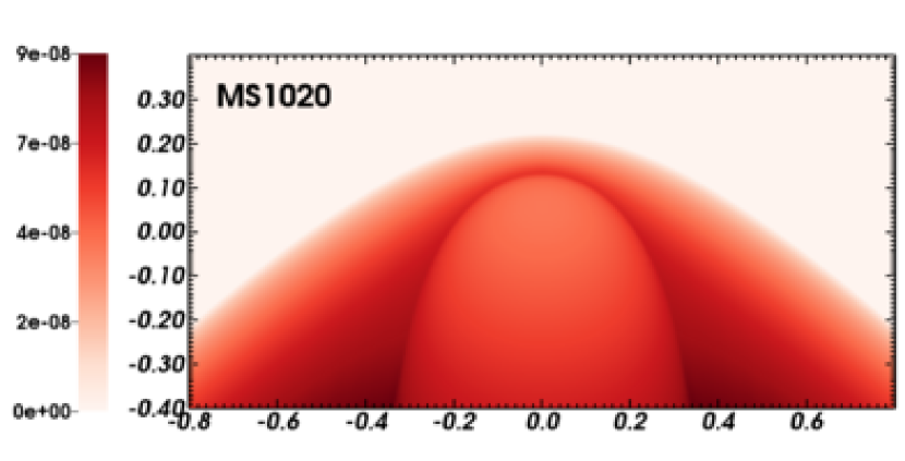
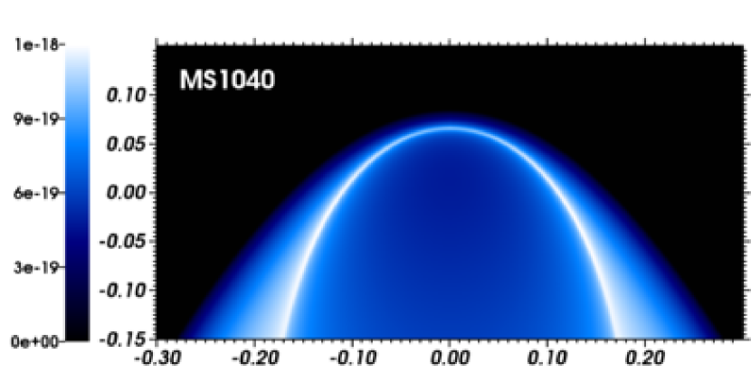
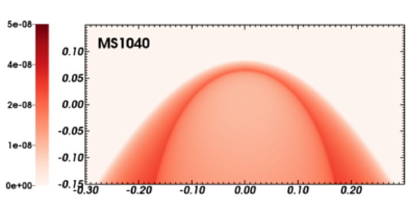
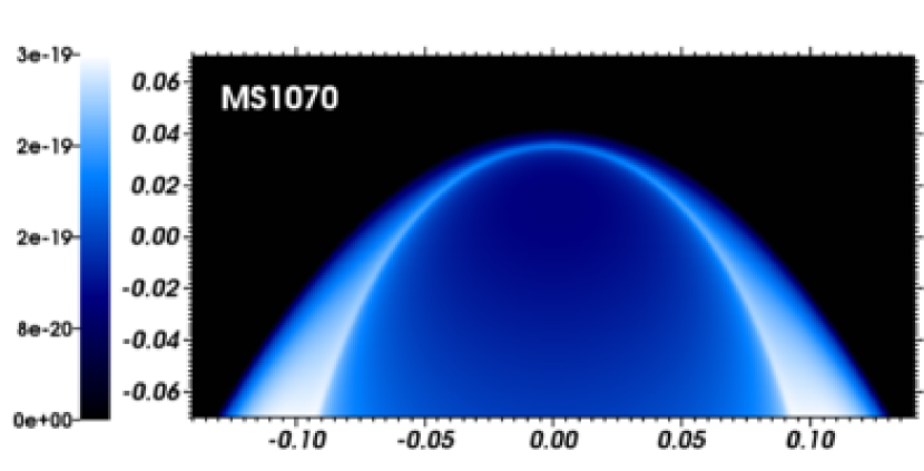
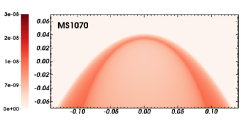
Figure 14: The figures show the H$\alpha$ surface brightness (left, in $\mathrm{erg}\,\mathrm{s}^{-1}\,\mathrm{cm}^{-2}\,\mathrm{arcsec}^{-2}$) and the dust surface mass density (right, in $\rm g\,\mathrm{cm}^{-2}$) for the bow shocks from the main sequence phase of our $10\,\mathrm{M}_{\odot}$ initial mass star. Quantities are calculated excluding the undisturbed ISM and plotted in the linear scale, as a function of the considered space velocities. The $x$-axis represents the radial direction and the $y$-axis the direction of stellar motion (in $\mathrm{pc}$). Only part of the computational domain is shown.

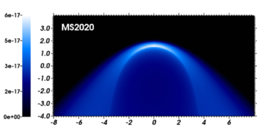
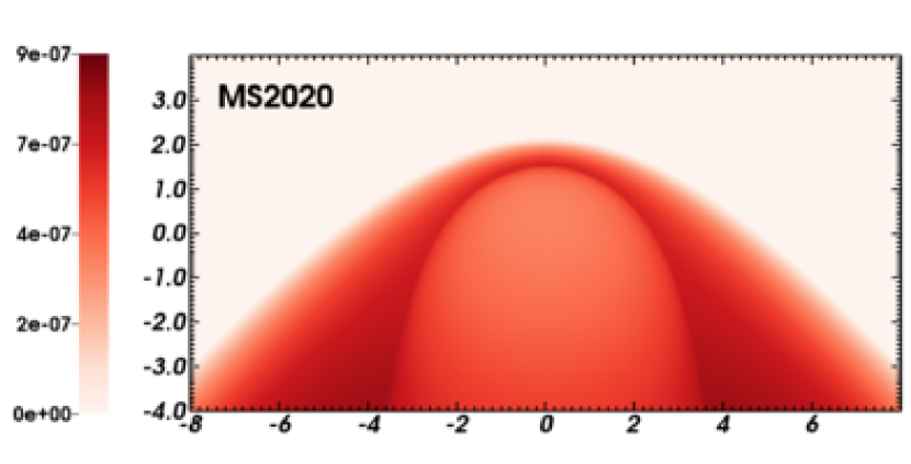
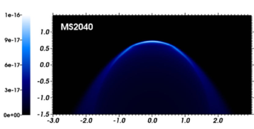
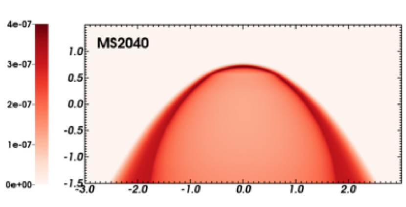
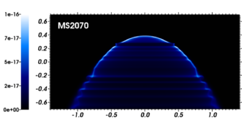
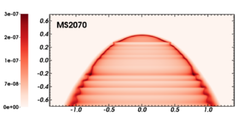
Figure 15: As Fig. 14, with an initial stellar mass of $20\,M_{\odot}$.

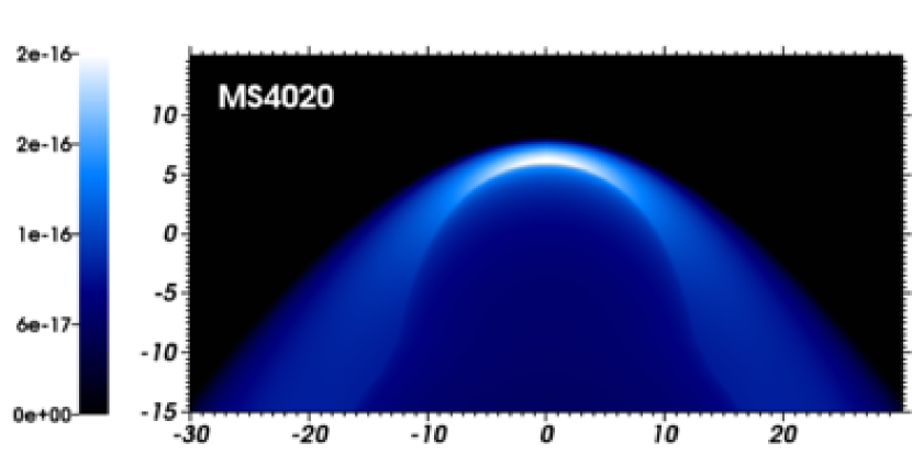
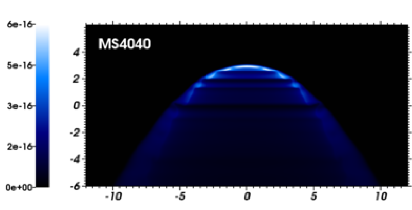
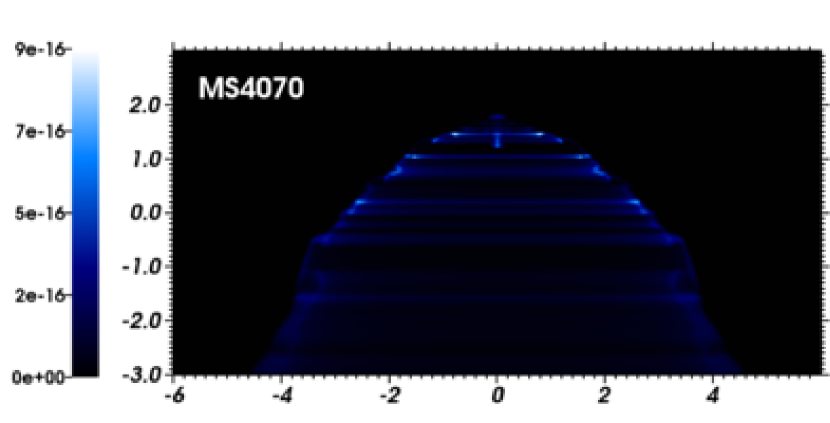
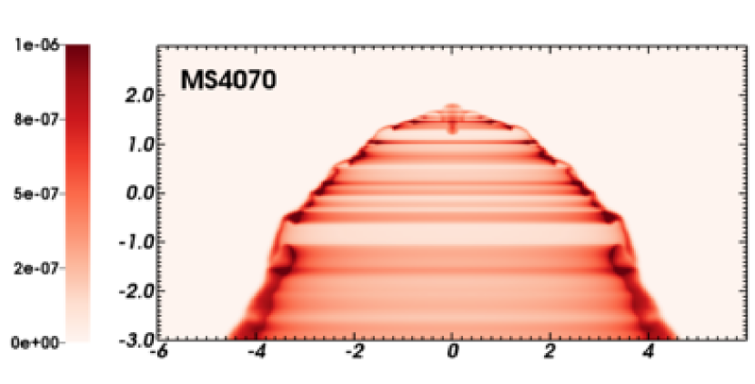
Figure 16: As Fig. 14, with an initial stellar mass of $40\,M_{\odot}$.

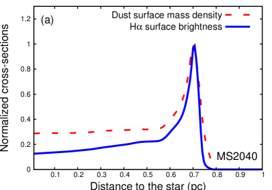
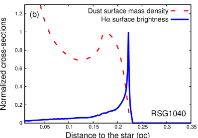
Figure 17: Normalized cross-sections taken along the direction of motion of the star, through the H$\alpha$ surface brightness and the dust surface mass density of the bow shock models MS2040 (a) and RSG1040 (b).

4 The stellar phase transition

In Fig. 18, we show the gas density field in our bow shock model of our initially $20\,M_{\odot}$ star moving with velocity $v_{\star}=40\,\mathrm{km}\,\mathrm{s}^{-1}$ during the stellar phase transition from the main sequence phase (top panel) to the red supergiant phase (bottom panel). The figures correspond to times $3.400$, $8.208$, $8.430$, $8.468$ and $8.500\,\rm Myr$, respectively.

The panel (a) of Fig. 18 shows the density field of the circumstellar medium during the main-sequence phase of our star (as in the middle panel of Fig. 7). When the main sequence phase ends, both the stellar mass-loss rate $\dot{M}$ and wind density $n_{\rm w}$ increase by more than an order of magnitude (see panel (e) of Fig. 3) so that the bow shock inflates and its stand-off distance doubles to reach about $1.7\,\rm pc$ (see panel (b) of Fig. 18). At about $8.350\,\rm Myr$, the wind velocity decreases rapidly and a shell of dense and slow red supergiant wind develops inside the bow shock from the main sequence phase (see panel (c) of Fig. 18). A double-arced structure forms at its apsis, as shown in the study detailing a model of Betelgeuse returning to the red supergiant phase after undergoing a blue loop  (Mackey et al., 2012). Under the influence of the stellar motion, the colliding shells expand beyond the forward shock of the main sequence bow shock and penetrate into the undisturbed ISM. The former bow shock recedes downwards from the direction of stellar motion because it is not supported by the ram pressure of the hot gas, whereas the new-born red supergiant bow shock adjusts itself to the changes in the wind parameters and a new contact discontinuity is established (see panel (d) of Fig. 18). After the phase transition, only the bow shock from the red supergiant phase remains in the domain (see panel (e) of Fig. 18).

As the star leaves the main sequence phase, the modifications of its wind properties affect the strengths of its termination and forward shocks. The decelerating wind slows the gas velocity by about 2 orders of magnitude in the post-shock region at the reverse shock. The hot bubble cools rapidly ($t_{\rm cool}\ll t_{\rm dyn}\ll t_{\rm cond}$) while the region of shocked wind becomes thicker and denser (see panels (c)-(d) of Fig. 3). The transfer of thermal energy by heat conduction ceases because there is no longer a sharp temperature change $\Delta T\geq 10^{7}\,\rm K$ across the contact discontinuity. Consequently, the position of the material discontinuity migrates from near the reverse shock to be coincident with the contact discontinuity (see the solid black line in panels (a) to (c) of Fig. 18). It sets up a dense and cold bow shock whose layer of shocked wind is thicker than the outer region of ISM gas (see panel (d) of Fig. 18).

The above described young bow shock of our initially $20\,M_{\odot}$ star is typical of the circumstellar medium of a runaway star undergoing a transition from a hot to a cold evolutionary phase. The phase transition timescale is longer for small $v_{\star}$ and shorter for high $v_{\star}$. The bow shocks generated by lower mass stars, e.g. our initially $10\,M_{\odot}$ star may be more difficult to observe because of their smaller and fainter shells. The wind parameters of our initially $10\,M_{\odot}$ star change more abruptly ($\sim 10^{4}\,\rm yr$, see panels (a) and (d) of Fig. 3), i.e. the preliminary increase of $\dot{M}$ and $n_{\rm w}$ is quicker and the subsequent inflation of their bow shock is much less pronounced. The slightly inflated bow shock from the main sequence phase has no time to reach a steady state before the transition happens (as in panel (b) in Fig. 18). Our slowly moving star with velocity $20\,\rm km\,\rm s^{-1}$ (i.e. the model RSG2020) has a supergiant phase that is shorter than the advection time of the hot bow shock, i.e. the former bow shock has not progressed downstream when the star ends its life (Section 5).

Our stellar phase transitions last $10^{4}-10^{5}\,\mathrm{yr}$, i.e. they are much shorter than both the main sequence and the red supergiant phases (see Fig. 3). This makes the direct observation of interacting bow shocks of stars in the field a rare event. Changes in the ambient medium can also affect the properties of bow shocks and wind bubbles, e.g. the so-called Napoleon’s hat which surrounds the remnant of the supernova SN1987A (Wampler et al., 1990; Wang & Wampler, 1992) and highlights the recent blue loop of its progenitor (Wang et al., 1993).

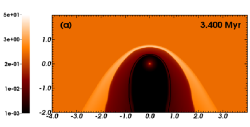
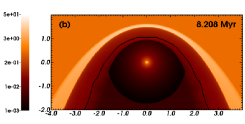
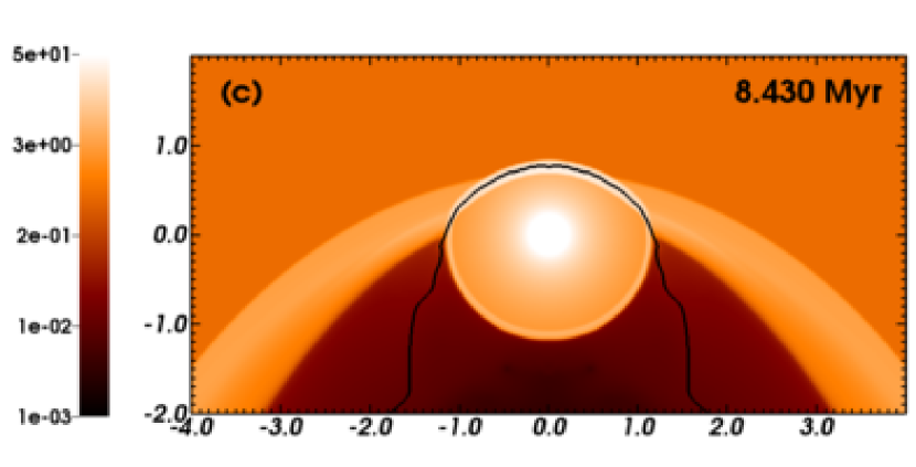
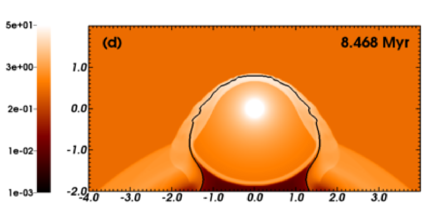
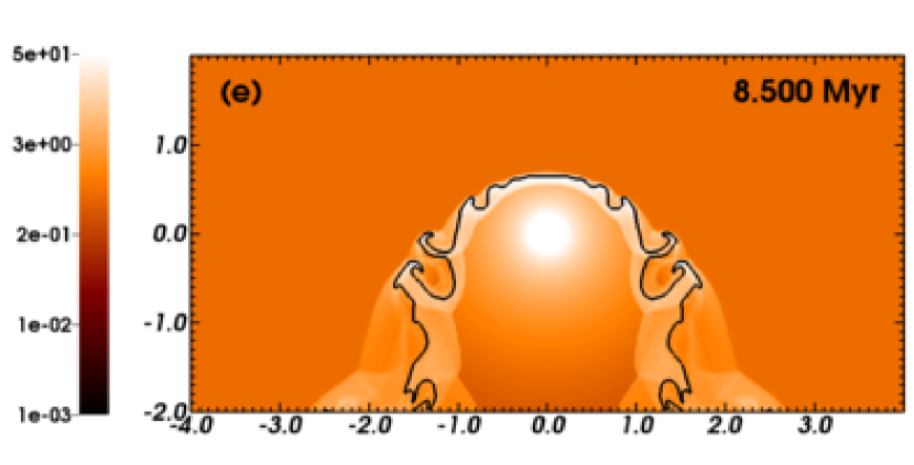
Figure 18: Time sequence of the stellar phase transition of the initially $20\,M_{\odot}$ star moving with $40\,\mathrm{km}\,\mathrm{s}^{-1}$. The figures show the transition from the main sequence phase (top panel) to the red supergiant phase (bottom panel) of the star. The gas number density is shown with a density range from $10^{-3}$ to $5.0\,\mathrm{cm}^{-3}$ in the logarithmic scale. The solid black contour traces the boundary between wind and ISM material $Q(\mn@boldsymbol{r})=1/2$. The $x$-axis represents the radial direction and the $y$-axis the direction of stellar motion (in $\mathrm{pc}$).

5 The red supergiant phase

5.1 Physical characteristics of the bow shocks

We show the gas density field in our bow shock models of the red supergiant phase RSG1020 ($10\,M_{\odot}$ initial stellar mass, $v_{\star}=20\,\mathrm{km}\,\mathrm{s}^{-1}$, upper panel), RSG1040 ($10\,M_{\odot}$, $40\,\mathrm{km}\,\mathrm{s}^{-1}$, middle panel) and RSG1070 ($10\,M_{\odot}$, $70\,\mathrm{km}\,\mathrm{s}^{-1}$, lower panel) in Fig. 19. Fig. 20 is similar for the $20\,M_{\odot}$ initial mass star. Figs. 19 and 20 show the contour $Q(\mn@boldsymbol{r})=1/2$ which traces the discontinuity between the wind and the ISM gas. $R(0)$ and $R(0)/R(90)$ are summarised for each panel in Table 2. The simulations were run until at least 40$\,t_{\rm cross}$ after the stellar phase transition, i.e. after the abrupt increase of $\dot{M}$ accompanied by a steep decrease of $v_{\rm w}$ (see panels (d)$-$(f) of Fig. 3).

The size of the bow shocks is predicted to scale as $\dot{M}^{1/2}$, $v_{\rm w}^{1/2}$ and $v_{\star}^{-1}$ according to Eq. (13) and Baranov et al. (1971). The scaling between simulations with $v_{\star}=40\,\rm km\,s^{-1}$ and $v_{\star}=70\,\rm km\,s^{-1}$ follows the prediction well, but deviations occur in the $v_{\star}=20\,\rm km\,s^{-1}$ simulations (see Table 2). The most deviating simulations either have a very weak shock preventing the forward shock from cooling and forming a thin shell (e.g. model RSG1020), or have not reached a steady state after the phase transition and consist of two interacting bow shocks (e.g. model RSG2020).

The thickness of the shocked layers depends on the cooling physics of the gas. Our simulations with $v_{\star}=20\,\rm km\,\rm s^{-1}$ have a roughly constant density across the material discontinuity. The reverse and forward shocks are weak without much heating and both layers can cool to about the same temperature. In models with $v_{\star}=40\,\rm km\,\rm s^{-1}$ the post-shock temperature at the forward shock is larger than for $v_{\star}=20\,\rm km\,s^{-1}$ and rapid cooling to $T\approx 10^{4}\,\rm K$ leads to a stronger compression of the material (see panel (b) and (d) of Fig. 12). At $v_{\star}=70\,\rm km\,s^{-1}$ the shocked ISM is a thin layer that has much lower density than the shocked wind (e.g. models RSG1070 and RSG2070). The forward shock is strong, therefore the hot shocked ISM has insufficient time to cool before it is advected downstream.

Our model RSG1020 with the weakest shocks is stable. Model RSG2020 has an expanding red supergiant wind that is replacing the previous main sequence shell. This simulation still has the remainder of the main sequence wind bow shock interacting with the bow shock from the red supergiant wind at the end of the star life. The contact discontinuity of the supergiant shell shows Rayleigh-Taylor fingers because of the density gradient between the old and new bow shocks. Our models with $v_{\star}\geq 40\,\rm km\,\rm s^{-1}$ have $v_{\rm w}\ll v_{\star}$ and so their bow shocks develop instabilities which distort dense and thin shells (Dgani et al., 1996b). The density field of the model RSG2070 resembles an isothermal bow shock with a distortion of the forward shock typical of the non-linear thin shell and transverse acceleration instabilities (Blondin & Koerwer, 1998). This instability arises because $R(0)$ is much larger than the cooling length in the shocked ISM and shocked wind.

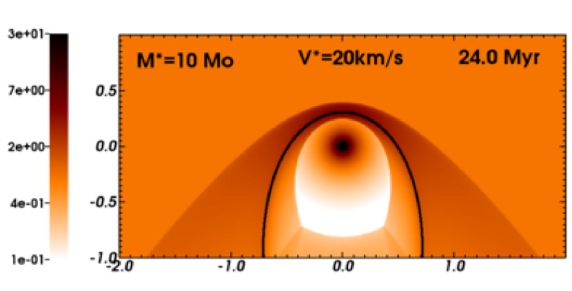
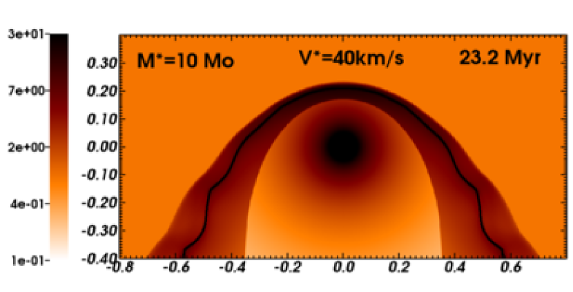
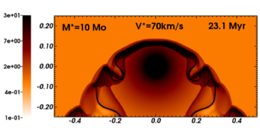
Figure 19: Grid of stellar wind bow shocks from the red supergiant phase of the $10\,M_{\odot}$ initial mass star according to the space velocity with respect to the ISM, with $20\,\mathrm{km}\,\mathrm{s}^{-1}$ (top panel), $40\,\mathrm{km}\,\mathrm{s}^{-1}$ (middle panel) and $70\,\mathrm{km}\,\mathrm{s}^{-1}$ (bottom panel). Models nomenclature follows Table 1. Gas number density is shown with a density range from $0.1$ to $30.0\,{\rm cm}^{-3}$ in the logarithmic scale. Note that the color scale is upset compared to Figs. 6, 7 and 8. The solid black contours trace the boundary between wind and ISM, $Q(\mn@boldsymbol{r})=1/2$. The $x$-axis represents the radial direction and the $y$-axis the direction of stellar motion (in $\mathrm{pc}$). Only part of the computational domain is shown.

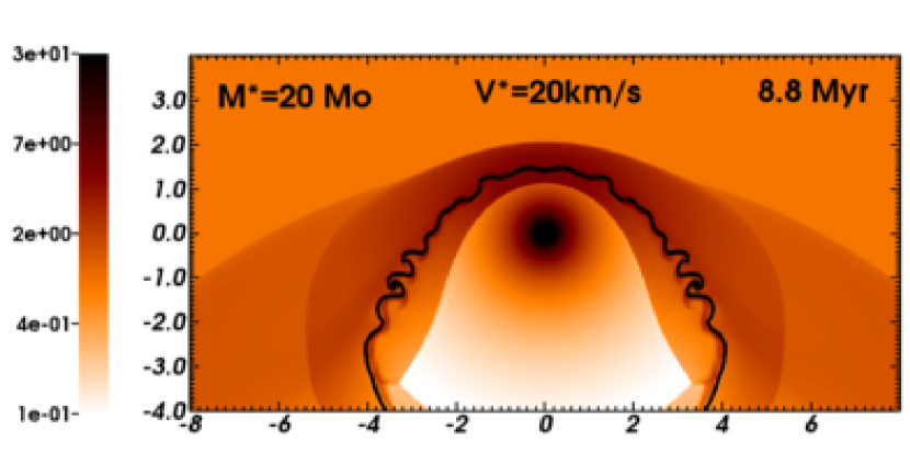
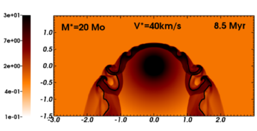
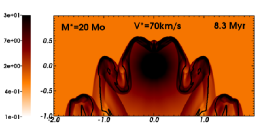
Figure 20: As Fig. 19, with an initial stellar mass of $20\,M_{\odot}$.

$R(0)/R(90)$ decreases at the contact discontinuity as a function of $v_{\star}$, e.g. $R(0)/R(90)\approx 0.6$ and $\approx 0.58$ for models RSG2020 and RSG2070, respectively. $R(0)/R(90)$ at the forward shock increases with $v_{\star}$ and $\dot{M}$, e.g. model RSG2020 and RSG2070 have $R(0)/R(90)\approx 0.46$ and $\approx 0.59$, respectively. These measures do not perfectly satisfy Wilkin’s solution, except for the models with $v_{\star}=70\,\rm km\,\rm s^{-1}$, although the ratios for the contact discontinuity are all within $10$ per cent of the analytic solution. Only the $v_{\star}=70\,\mathrm{km}\,\mathrm{s}^{-1}$ simulations, with their thin bow shocks that come closest to the isothermal limit, have forward shocks that satisfy $R(0)/R(90)\approx 1/\sqrt{3}$ (see Fig. 20).

Because the temperature jumps are small across the interfaces and shocks in the bow shocks around red supergiants, e.g. $\mathit{\Delta}T\approx 10^{3}\,\rm K$ at the reverse shock and $\mathit{\Delta}T\approx 4\times 10^{4}\,\rm K$ at the forward shock of model RSG1040, thermal conduction is not important. The bow shocks around red supergiants therefore have coincident contact and material discontinuities (see black contours in Figs. 21 and 22).

Table 3: Stellar and bow shock luminosities. $L_{\star}$ represents the stellar luminosity at the end of each simulation, $L_{\rm gas}$ is the bow shock luminosity from optically-thin cooling of the gas, and $L_{\rm wind}$ the part of $L_{\rm gas}$ originating from the wind material. $L_{\rm H\alpha}$ is the luminosity of H$\alpha$ emission and $L_{\rm FL}$ is the luminosity generated for photoionized bow shocks by cooling from [O ii] and [O iii] forbidden lines emission is the range of $\approx 8000\leq T\leq 6.0\times 10^{4}\,\rm K$. $L_{\rm IR}$ is the infrared luminosity, calculated on the basis of reemission of starlight by the dust grains (our Appendix B). $\widetilde{\mathit{\Gamma}}_{\alpha}$ represents the radiative heating of the gas (see Eq. 19).

${\rm{Model}}$	$L_{\star}\,(\rm erg\,s^{-1})$	$L_{\rm gas}\,(\rm erg\,s^{-1})$	$L_{\rm wind}\,(\rm erg\,s^{-1})$	$L_{\rm H\alpha}\,(\rm erg\,s^{-1})$	$L_{\rm FL}\,(\rm erg\,s^{-1})$	$L_{\rm IR}\,(\rm erg\,s^{-1})$	$\widetilde{\mathit{\Gamma}}_{\alpha}\,(\rm erg\,s^{-1})$
MS1020	$2.42\times 10^{37}$	$1.39\times 10^{31}$	$4.66\times 10^{24}$	$9.00\times 10^{29}$	$1.26\times 10^{31}$	$2.10\times 10^{33}$	$5.32\times 10^{30}$
MS1040	$2.42\times 10^{37}$	$6.17\times 10^{30}$	$1.55\times 10^{25}$	$4.10\times 10^{28}$	$5.75\times 10^{30}$	$7.00\times 10^{32}$	$2.53\times 10^{29}$
MS1070	$2.42\times 10^{37}$	$4.70\times 10^{30}$	$1.76\times 10^{25}$	$2.40\times 10^{27}$	$3.53\times 10^{30}$	$3.50\times 10^{32}$	$1.21\times 10^{28}$
RSG1020	$7.66\times 10^{37}$	$1.36\times 10^{32}$	$1.35\times 10^{32}$	$1.60\times 10^{27}$	$-$	$6.20\times 10^{33}$	$2.27\times 10^{30}$
RSG1040	$7.32\times 10^{37}$	$1.35\times 10^{32}$	$1.30\times 10^{30}$	$7.10\times 10^{28}$	$-$	$1.30\times 10^{34}$	$3.62\times 10^{28}$
RSG1070	$7.32\times 10^{37}$	$3.50\times 10^{32}$	$1.73\times 10^{30}$	$7.50\times 10^{28}$	$-$	$2.40\times 10^{34}$	$2.30\times 10^{28}$
MS2020	$2.59\times 10^{38}$	$6.60\times 10^{33}$	$7.50\times 10^{27}$	$1.30\times 10^{33}$	$5.57\times 10^{33}$	$2.10\times 10^{35}$	$7.90\times 10^{33}$
MS2040	$2.16\times 10^{38}$	$2.48\times 10^{33}$	$6.83\times 10^{27}$	$1.90\times 10^{32}$	$2.17\times 10^{33}$	$6.20\times 10^{34}$	$1.00\times 10^{33}$
MS2070	$1.64\times 10^{38}$	$2.32\times 10^{33}$	$6.18\times 10^{28}$	$3.60\times 10^{31}$	$1.69\times 10^{33}$	$2.40\times 10^{34}$	$2.20\times 10^{32}$
RSG2020	$5.94\times 10^{38}$	$2.46\times 10^{32}$	$4.70\times 10^{31}$	$9.70\times 10^{27}$	$-$	$1.30\times 10^{36}$	$1.34\times 10^{31}$
RSG2040	$5.18\times 10^{38}$	$1.56\times 10^{33}$	$1.80\times 10^{31}$	$7.10\times 10^{29}$	$-$	$4.30\times 10^{35}$	$1.42\times 10^{31}$
RSG2070	$5.95\times 10^{38}$	$3.65\times 10^{33}$	$2.04\times 10^{31}$	$1.70\times 10^{30}$	$-$	$1.20\times 10^{36}$	$9,98\times 10^{30}$
MS4020	$1.30\times 10^{39}$	$3.90\times 10^{35}$	$8.00\times 10^{29}$	$8.30\times 10^{34}$	$3.30\times 10^{35}$	$4.00\times 10^{36}$	$4.76\times 10^{35}$
MS4040	$1.03\times 10^{39}$	$1.00\times 10^{35}$	$3.70\times 10^{29}$	$1.60\times 10^{34}$	$8.74\times 10^{34}$	$1.20\times 10^{36}$	$9.10\times 10^{34}$
MS4070	$9.00\times 10^{38}$	$5.40\times 10^{34}$	$2.80\times 10^{29}$	$2.80\times 10^{33}$	$4.46\times 10^{34}$	$4.50\times 10^{35}$	$1.60\times 10^{34}$

5.2 Bow shock emissivity

5.2.1 Luminosities

The luminosities $L_{\rm gas}$, $L_{\rm wind}$, $L_{\rm H\alpha}$ and $L_{\rm IR}$ of the bow shocks generated by our red supergiant models are plotted as a function of $\dot{M}$ and $v_{\star}$ in panel (b) of Fig. 13. As is the case for bow shocks produced by main sequence stars, $L_{\rm gas}$ is influenced by $v_{\star}$ and by the size of the bow shock. $L_{\rm gas}\,\propto n^{2}$ and slightly increases with $v_{\star}$ because the compression factor of the shell is larger for high $v_{\star}$. The variations in size drive the increase of $L_{\rm gas}$ as a function of $\dot{M}$ if $v_{\star}$ is fixed. In contrast to the bow shocks around main sequence stars, the increase of $L_{\rm gas}$ seen in panel (b) of Fig. 13 for a given model triplet shows that the luminosity is more influenced by the density than by the volume of the bow shocks.

$L_{\rm wind}$ is several orders of magnitude dimmer than $L_{\rm gas}$, e.g. $L_{\rm wind}/L_{\rm gas}\approx 10^{-2}$ for model RSG1040, i.e. the wind contribution is negligible compared to the luminosity of the shocked ISM gas. The difference between $L_{\rm wind}$ and $L_{\rm gas}$ is less than in our main sequence models because the gas cooling behind the slow red supergiant reverse shock is efficient. Model RSG1020 behaves differently because even though it scales in volume with model RSG1040, its small $v_{\star}$ results in a weak forward shock which is cool so there is little cooling in the shocked ISM ($L_{\rm wind}\sim L_{\rm gas}$). The total bow shock luminosity of optically-thin radiation of model RSG2020 is increased by a contribution from the former main sequence bow shock around the forming red supergiant shell (see upper panel of Fig. 20).

The bow shock luminosity of H$\alpha$ emission is negligible compared to the total bow shock luminosity, e.g. $L_{\rm H\alpha}/L_{\rm gas}\approx 10^{-3}$$-$$10^{-5}$, see lower panel of Fig. 13. $L_{\rm H\alpha}$ increases with $v_{\star}$, e.g. $L_{\rm H\alpha}\approx 7.1\times 10^{29}$ and $\approx 1.7\times 10^{30}\,\mathrm{erg}\,\mathrm{s}^{-1}$ for model RSG2040 and RSG2070, respectively. The H$\alpha$ emission of the bow shocks for the $10$ and $20\,\rm M_{\odot}$ stars differs by $\approx 1$ order of magnitude. Models RSG1020 and RSG2020 have little H$\alpha$ emission because their weak forward shocks do not ionize the gas significantly and prevent the formation of a dense shell.

The infrared luminosity is such that $L_{\rm IR}\gg L_{\rm gas}$. This is because of the fact that $L_{\rm IR}$ provides an upper limit for the infrared light (our Appendix B) and because the circumstellar medium around red supergiants is denser than that during the main sequence phase, i.e. there is a lot of dust from the stellar wind in these bow shocks that can reprocess the stellar radiation. $L_{\rm IR}$ increases by about two orders of magnitude between the $10$ and $20\,\rm M_{\odot}$ models if $v_{\star}$ is considered fixed, which is explained by their different wind and bow shock densities (see Figs. 19 and 20). Model RSG2020 does not fit this trend because the huge mass of the bow shock of the previous evolutionary phase affects its luminosity $L_{\rm IR}\approx 1.3\times 10^{36}\,\mathrm{erg}\,\mathrm{s}^{-1}$. The enormous infrared luminosity of bow shocks around red supergiants compared to their optically-thin gas radiation suggests that they should be more easily observed in the infrared than in the optical bands and partly explains why the bow shock around Betelgeuse was discovered in the infrared.

5.2.2 Synthetic emission maps

Figs. 21 and 22 show the bow shock H$\alpha$ surface brightness (left panels) and dust surface mass density (right panels) for our $10$ and $20\,M_{\odot}$ models, respectively. Each figure shows $v_{\star}=20\,\rm km\,\rm s^{-1}$ (top), $v_{\star}=40\,\rm km\,\rm s^{-1}$ (middle) and $v_{\star}=70\,\rm km\,\rm s^{-1}$ (bottom). For red supergiants we assume that both the stellar wind and the ISM gas include dust (our Appendix B).

In our models the H$\alpha$ emission of bow shocks produced by red supergiants originates from the shocked ISM in the post-shock region at the forward shock. The region of maximum emission is at the apex of the structure for simulations with $v_{\star}=20\,\rm km\,\rm s^{-1}$ and is extended to the tail as $v_{\star}$ increases, e.g. for the model RSG1040. The surface brightness increases with $v_{\star}$ and $\dot{M}$ because the post-shock temperature at the forward shock increases when the shocks are stronger. However, the H$\alpha$ emission is fainter by several orders of magnitude than our bow shock models for hot stars (see Figs. 14 and 21). As a consequence, these bow shocks are not likely to be observed in H$\alpha$ because their H$\alpha$ surface brightnesses is below the detection sensitivity of the SHS (Parker et al., 2005).

Panel (b) of Fig. 17 plots the normalized cross-sections taken from the H$\alpha$ surface brightness and the dust surface mass density of the bow shock model RSG1020. The H$\alpha$ emission is maximum in the post-shock region at the forward shock, whereas the dust surface density peaks in the post-shock region at the reverse shock of the bow shock. All our models for bow shocks for red supergiants exhibit such comportment which suggests that H$\alpha$ and infrared emission do not originate from the same region of the bow shock. Because the red supergiant wind is denser than the ISM, most of the infrared emission probably originates from the shocked wind.

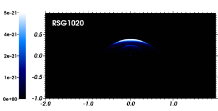
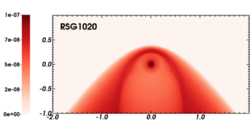
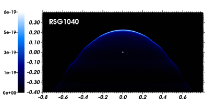
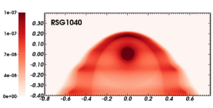
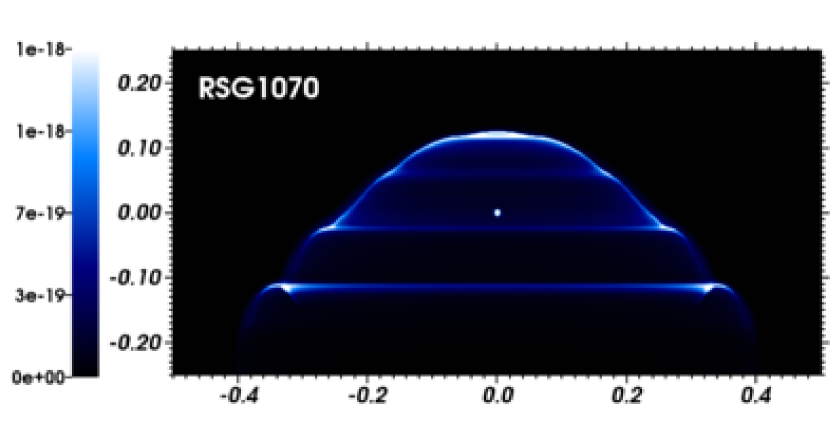
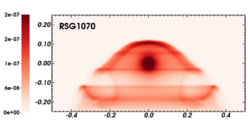
Figure 21: The figures show the H$\alpha$ surface brightness (left, in $\mathrm{erg}\,\mathrm{s}^{-1}\,\mathrm{cm}^{-2}\,\mathrm{arcsec}^{-2}$) and the dust surface mass density (right, in $\rm g\,\mathrm{cm}^{-2}$) for the bow shocks from the red supergiant phase of our $10\,\mathrm{M}_{\odot}$ initial mass star. Quantities are calculated excluding the undisturbed ISM and plotted in the linear scale, as a function of the considered space velocities. The $x$-axis represents the radial direction and the $y$-axis the direction of stellar motion (in $\mathrm{pc}$). Only part of the computational domain is shown.

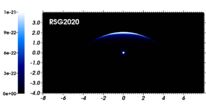
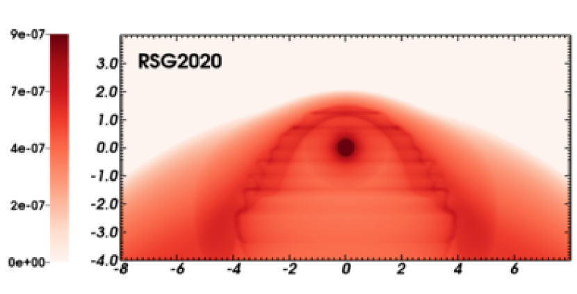
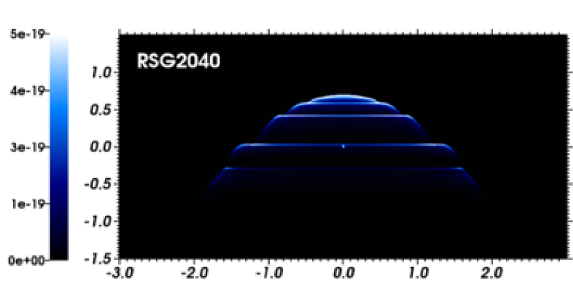
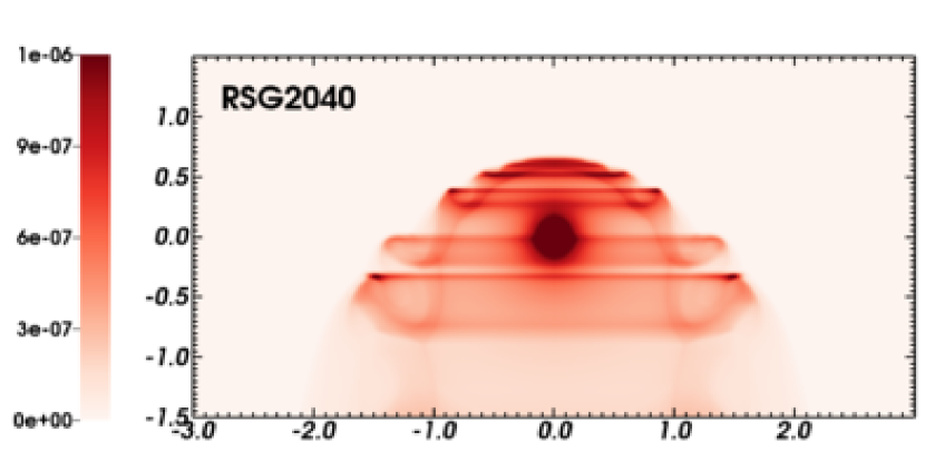
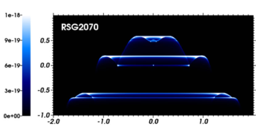
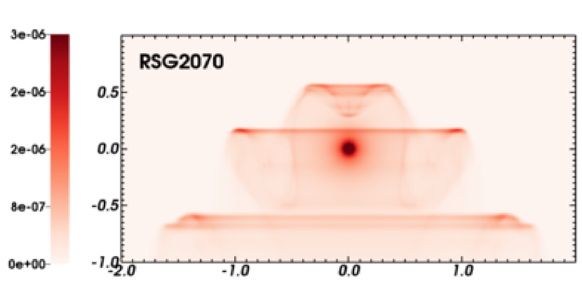
Figure 22: As Fig. 21, with an initial stellar mass of $20\,M_{\odot}$.

6 Discussion

6.1 Comparison with previous works

6.1.1 Bow shocks around main sequence stars

We carried out tests with two numerical methods to integrate the parabolic term associated with heat conduction: the explicit method used in Comerón & Kaper (1998) and the Super-Time-Step method (Alexiades et al., 1996). The results are consistent between the two methods, except that the explicit scheme is less diffusive but also extremely time consuming. We adopt the Super-Time-Step algorithm given that the spatial resolution of our models is better than in Comerón & Kaper (1998).

We tested this method using the code pluto with respect to the models in Comerón & Kaper (1998). Our simulations support their study in that all the bow shocks are reproduced reasonably well. Our simulations that aim to reproduce the highly unstable simulation cases C (bow shock with strong wind) and E (bow shock in high density ambient medium) in Comerón & Kaper (1998) are slightly more affected by the development of overdensities at the apex of the structure which later govern the shape of the instabilities which distort the whole bow shocks. Our results vary depending on the chosen coordinate system and the interpolation scheme used at the symmetry axis. We conclude that instabilities growing at the apsis are artificially confined near $R=0$ by the rotational symmetry imposed by the coordinate system.

Our models with $v_{\star}=20\,\rm km\,\rm s^{-1}$ produce weak bow shocks. Such bow shocks correspond to the Case A model in Comerón & Kaper (1998), which uses a similar wind velocity ($\sim 1000\,\rm km\,\rm s^{-1}$), and a mass-loss rate of $10^{-7}\,\rm M_{\odot}\,\rm yr^{-1}$ (i.e. 1.5 orders of magnitude larger, similar and one order of magnitude smaller than our $10$, $20$ and $40\,\rm M_{\odot}$ stars, respectively), a less dense ISM ($0.1\,\rm cm^{-3}$) and a much higher $v_{\star}$ ($\approx 100\,\rm km\,\rm s^{-1}$). Our models include cooling by forbidden collisionally excited lines and assume the same $T_{\rm ISM}\approx 8000\,\rm K$ as their Case A. These models are similar because their weak forward shocks do not allow the gas to cool rapidly and they all have a region of shocked ISM thicker than the hot bubble along the direction of motion of the star, as signified by the absence of a sharp density peak in the region of shocked ISM in panel (a) of Fig. 12, compared to lower panel of fig. 7 in Comerón & Kaper (1998).

Our models MS4040 and MS4070 have strong shocks and are similar to the Case C model in Comerón & Kaper (1998). Their case C uses a higher $v_{\rm w}\approx 3000\,\rm km\,\rm s^{-1}$, a slightly larger $\dot{M}\sim 10^{-6}\,\rm M_{\odot}\,\rm yr^{-1}$, a less dense ISM ($0.1\,\rm cm^{-3}$) and a higher $v_{\star}$ ($\approx 100\,\rm km\,\rm s^{-1}$). The combination of high $v_{\star}$ and high $v_{\rm w}$ induces a strong compression factor at the forward shock where the gas cools rapidly and reduces the thickness of the shocked ISM into a thin, unstable shell. These models best fit analytical approximations of an infinitely thin bow shock (Comerón & Kaper, 1998).

We conclude that for overlapping parameters, i.e. for similar $\dot{M}$ and $v_{\star}$, our results agree well with existing models in terms of bow shock morphology and stability. We extend the parameter space for stars with weak winds, $\dot{M}\approx 10^{-9.5}$ in our $10\,M_{\odot}$ model and use the typical particle density of the Galactic plane.

6.1.2 Bow shocks around red supergiants

We tested our numerical setup to reproduce the double bow shock around Betelgeuse (Mackey et al., 2012). Including heat conduction did not significantly change the results and we successfully reproduced the model using the same cooling curve as in Mackey et al. (2012). The simulations of red supergiant bow shocks of Mohamed et al. (2012) used a more precise time-dependent cooling network (Smith & Rosen, 2003) and, because of their Lagragian nature, these models are intrinsically better in terms of spatial resolution. To produce more detailed models which can predict emission line ratio is beyond the scope of this study but could be achieved using the native multi-ion non-equilibrium cooling module of the code pluto (Teşileanu et al., 2008).

Model RSG2020 shows a weak bow shock with a dense and cold shell expanding into the former hot and smooth bow shock. Rayleigh-Taylor instabilities develop at the discontinuity between the two colliding bow shocks as in the model of Betelgeuse’s multiple arched bow shock in Mackey et al. (2012).

Our simulations with $v_{\star}=40\,\rm km\,\rm s^{-1}$ show radiative forward shocks and unstable contact discontinuities. Model RSG1040 resembles the simulations of van Marle et al. (2011) and Decin et al. (2012) which have a similar $\dot{M}\approx 3\times 10^{-6}\,\rm M_{\odot}\,\rm yr^{-1}$ but a smaller $v_{\star}\approx 28\,\rm km\,s^{-1}$ and denser ISM ($2\,\rm cm^{-3}$). We do not use the two-fluid approach of van Marle et al. (2011) which allows the modelling of ISM dust grains and explains the differences in terms of stability of the contact discontinuity. Their simulation with type 1 grains is more unstable than our model RSG1040, probably because they use a denser ISM. Model RSG2040 has a thinner region of shocked ISM compared to the region of shocked wind which makes this model unstable. The instabilities of model RSG2040 are similar to the clumpy forward shock of models A-C in Mohamed et al. (2012) which have larger $\dot{M}$ and a denser medium.

Our simulations with $v_{\star}=70\,\rm km\,\rm s^{-1}$ show the largest compression. Model RSG2070 has a strongly turbulent shell with dramatic instabilities, consistent with the high $v_{\star}$ and high Mach number model in Blondin & Koerwer (1998). Our model RSG2070 illustrates the transverse acceleration instability where an isotropically expanding wind from the star meets the collinear ISM flow and pushes the developing eddies sidewards. Model RSG2070 is different from the model D with cooling of Mohamed et al. (2012) which has a similar $v_{\star}\approx 72.5\,\rm km\,s^{-1}$ but a weaker wind $\dot{M}\approx 3.1\times 10^{-6}\,\rm M_{\odot}\,\rm{yr}^{-1}$. Because of its particular initial conditions, i.e. a hotter and diluted ISM with $n\approx 0.3\,\rm cm^{-3}$ and $T_{\rm ISM}\approx 8000\,\rm K$, the gas does not cool efficiently at the forward shock and the post-shock regions of the bow shock remain isothermal, see right panel of fig. 10 of Mohamed et al. (2012).

With similar model parameters, our results agree well with the existing models and we conclude that heat conduction is not mandatory to model bow shocks from cool stars. Because we neglect the effects of dust dynamics on the bow shocks stability, our models differ slightly from existing models with $v_{\star}\approx 30$$-$$40\,\rm km\,\rm s^{-1}$. However, this does not concern the overall shape of the bow shocks but rather the (in)stability of their contact discontinuities. We extended the parameter space by introducing models with $v_{\star}=20\,\rm km\,\rm s^{-1}$.

6.2 On the observability of bow shocks from massive runaway stars

Fig. 23 plots the luminosities of our bow shock models for main sequence (top panels) and red supergiant (bottom panels) stars as a function of $M_{\star}$ and $v_{\star}$. With respect to their optically-thin gas radiation, the brightest bow shocks produced by main-sequence stars are generated by the more massive stars moving with a slow space velocity, e.g. the $40\,M_{\odot}$ main sequence star moving with $v_{\star}=20\,\rm km\,\rm s^{-1}$, and the brightest bow shocks produced by red supergiants are generated by the more massive star of our sample, moving at high space velocity i.e. a $20\,M_{\odot}$ red supergiant moving with $v_{\star}=70\,\rm km\,\rm s^{-1}$ (see panels (a) and (d) of Fig. 23). The same points arise from the luminosity of H$\alpha$ emission (see panels (b) and (e) of Fig. 23). The infrared luminosity indicates that the brightest bow shocks generated by a main sequence star are produced by high mass, low velocity stars (see panel (c) in Fig. 23). Concerning the bow shocks generated by red supergiants, their infrared luminosities suggest that the brightest are produced by high-mass stars moving at either low or high space velocities (see panel (f) in Fig. 23).

Because $L_{\rm IR}$ is larger than $L_{\rm H\alpha}$ or $L_{\rm gas}$, the infrared waveband is the most appropriate to search for stellar-wind bow shocks around main sequence and red supergiant stars. According to our study, bow shocks produced by high mass main sequence stars moving with low space velocities should be the easiest ones to observe in the infrared. The most numerous runaway stars have a low space velocity (Eldridge et al., 2011) and consequently bow shocks produced by high-mass red supergiants moving with low space velocity are the most numerous ones, and the probability to detect one of them is larger. Many stellar wind bow shocks surrounding hot stars ejected from stellar cluster are detected by means of their $\leq 24\,\mu m$ infrared signature (see Gvaramadze et al., 2010, 2011). Because our study focuses on the most probable bow shocks forming around stars exiled from their parent cluster, we expect them to be most prominent in that waveband.

Fig. 24 plots the bow shock luminosities for our main sequence models as a function of $R(0)^{3}$. It shows a strong scaling relation between the luminosities and the volume of the bow shocks, i.e. the brightnesses of these bow shocks are governed by the wind momentum. The optical luminosities of our red supergiant models do not satisfy these fits because the gas is weakly ionized. This behaviour concerns the overall luminosities of the bow shocks, not their surface brightnesses. Furthermore, this statement is only valid for the used ISM density, and some effects may make them dimmer, e.g. a lower density medium increasing their volume $\sim R(0)^{3}\sim 1/\sqrt{n_{\rm ISM}^{3}}$.

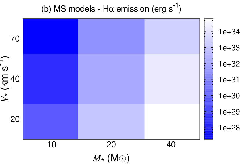
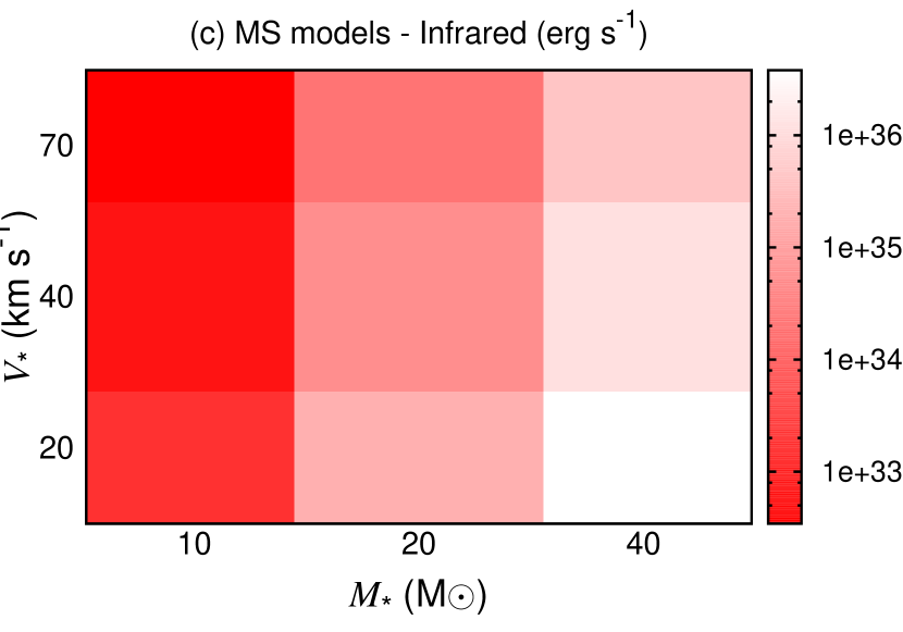
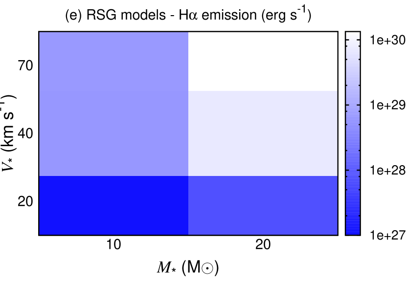
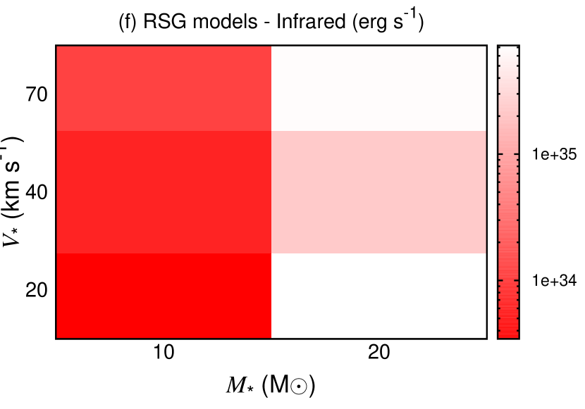
Figure 23: Bow shocks luminosities (in $\rm erg\,\rm s^{-1}$) in our main sequence (top panels) and red supergiant (bottom panels) models. We show the luminosity of optically-thin cooling (left green panels), H$\alpha$ emission (middle blue panels) and reprocessed infrared starlight by dust grains (right red panels) of Table 3. On each plot the $x$-axis is the initial mass $M_{\star}$ (in $M_{\odot}$) and the $y$-axis is the space velocity $v_{\star}$ (in $\rm km\,\rm s^{-1}$) of our runaway stars.

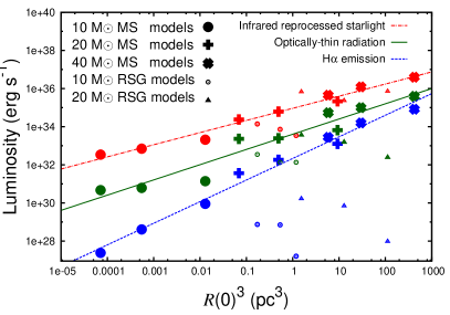
Figure 24: Bow shocks luminosities (in $\rm erg\,\rm s^{-1}$) as a function of $R(0)^{3}$ (in $\rm{pc}^{3}$) for the main sequence (large symbols) and red supergiant models (small symbols). The overplotted thin lines are least square fits of the luminosity of optically-thin gas radiation (solid green line), the infrared luminosity of reprocessed starlight (dashed red line) and the luminosity of H$\alpha$ emission (dotted blue line).

7 Conclusion

We present a grid of hydrodynamical models of bow shocks around evolving massive stars. The runaway stars initial masses range from $10$ to $40\,\mathrm{M}_{\odot}$ and their space velocities range from $20$ to $70\,\mathrm{{km}\,s^{-1}}$. Their evolution is followed from the main sequence to the red supergiant phase. Our simulations include thermal conduction and distinguish the treatment of the optically-thin cooling and heating as a function of the evolutionary phase of the star.

Our results are consistent with Comerón & Kaper (1998) in that our bow shocks show a variety of shapes which usually do not fit a simple analytic approximation (Wilkin, 1996). We stress the importance of heat conduction to model the bow shocks around main sequence stars and find that this is not an important process to explain the morphology of bow shocks around red supergiants. We underline its effects on their morphology and structure, especially concerning the transport of ISM material to the hot region of the bow shocks generated by hot stars. The heat transfer enlarges the bow shocks and considerably reduces the volume of shocked wind so that optical emission mainly originates from shocked ISM material. We extend the analysis of our results by calculating the luminosities of the bow shocks and detail how they depend on the star’s mass loss and space velocity.

Our bow shock models of hot stars indicate that the main coolants governing their luminosities are the optical forbidden lines such as [O ii] and [O iii]. The luminosity of optical forbidden lines is stronger than the luminosity of H$\alpha$ emission, which only represents less than a tenth of the luminosity by optically-thin radiation. This agrees with the observations of Gull & Sofia (1979) who noticed that [O iii] is the strongest optical emission line of the bow shock of $\zeta$ Oph. Our study also shows that those forbidden emission lines are fainter than the infrared emission of bow shocks produced by main sequence stars.

Our bow shock models with hot stars are brightest in H$\alpha$ in the cold shocked ISM material near the contact discontinuity. Because their dust surface mass density peaks at the same distance to the star as their H$\alpha$ emission, we suggest that their infrared emission is also maximum at the contact discontinuity. The H$\alpha$ surface brightness is maximum upstream from the star for small space velocities and are extended downstream from the star for larger velocities. Our bow shock models can have H$\alpha$ surface brightnesses above the detection threshold of the SuperCOSMOS H-alpha Survey (Parker et al., 2005).

Our bow shocks generated by red supergiants have a large infrared luminosity. Their luminosity by optically-thin radiative cooling mainly originates from shocked ISM material, whereas our models indicate that their infrared luminosity principally comes from regions of shocked wind. The H$\alpha$ emission of our bow shocks around cool stars originates from their forward shock. Its maximum is upstream from the star in the supersonic regime and is lengthened in the wake of the bow shock in the hypersonic regime. Their H$\alpha$ emission is negligible compared to their luminosity of optically-thin radiation because their gas is weakly ionized. In conclusion, these bow shocks are more likely to be observed in the infrared than in the optical or in H$\alpha$. This supports the hypothesis that the optically-detected bow shock of IRC$-$10414 is photoionized by an external source because the collisionally excited [N ii] line in the shocked wind is brighter than the H$\alpha$ emission at the forward shock (Meyer et al., 2014).

We also conclude that bow shocks produced by runaway main sequence and red supergiants should be easier to detect in the infrared. The brightest and most easily detectable bow shocks from main sequence stars are those of high mass stars ($\approx\,40\,M_{\odot}$) with small space velocity ($\approx\,20\,\rm km\,\rm s^{-1}$). With the ISM density of the Galactic plane, their luminosities are governed by their wind momentum and they scale monotonically with their volume. In the infrared, the most probable bow shocks to detect around red supergiants are produced by high mass ($\approx\,20\,M_{\odot}$) stars with small space velocity ($\approx\,20\,\rm km\,\rm s^{-1}$).

The hereby presented grid of models will be enlarged in a wider study, and forthcoming work will investigate the effects of an ISM background magnetic field. We also plan to focus on the latest stellar evolutionary stage in order to model the final explosion happening at the end of the massive star life, because the supernova ejecta interact with the shaped circumstellar medium.

Appendix A Emission maps and projected dust mass

The simulations are post-processed in order to obtain projected H$\alpha$ emission maps and ISM dust projected mass. The gas $T$ is calculated according to Eq. (5). For every cell of the computational domain and for a given quantity $\xi(T)$ of units $[\xi]$ representing either rate of emission (in $\rm erg\,s^{-1}\,cm^{-3}$) or a density (in $\rm g\,cm^{-3}$) we calculate its projection $\mathcal{P}_{\xi}$. The integral of $\xi$ is performed inside the bow shock along a path perpendicular to the plane ($O,R,z$), excluding the unperturbed ISM. Taking into account the projection factor, it is,

$$\mathcal{P}_{\xi}(R,z)=2\int_{R^{{}^{\prime}}=R}^{R^{{}^{\prime}}=R_{max}}\xi(R^{{}^{\prime}},z)\frac{R^{{}^{\prime}}dR^{{}^{\prime}}}{\sqrt{R^{{}^{\prime}2}-R^{2}}}\,[\xi]\,\rm cm.$$ (20)

For hot, photoionized medium we use the H$\alpha$ emissivity rate interpolated from the Table 4.4 of Osterbrock & Bochkarev (1989), which is,

$$\xi(T)\approx 1.21\times 10^{-22}T^{-0.9}n_{\rm e}n_{\rm p}\,\rm erg\,s^{-1}\,cm^{-3}\,sr^{-1},$$ (21)

where $n_{\rm e}$ and $n_{\rm p}$ are the number of electrons and protons per unit volume, respectively. For cool, CIE medium we employ a similar formalism, taking into account the fact that only the ions emit, i.e. the emission is proportional to $n_{\rm e}n_{\rm i}$ with $n_{\rm i}$ the number of ions per unit volume. The emission rate is,

$$\xi(T)\approx 1.21\times 10^{-22}T^{-0.9}n_{\rm i}n_{\rm e}\,\rm erg\,s^{-1}\,cm^{-3}\,sr^{-1}.$$ (22)

The ISM projected dust mass is calculated integrating the number density. For a dust-to-gas ratio $X_{\rm d/\rm g}$ and for the total gas number density $n$, its expression is,

$$\xi(T)=nX_{\rm d/\rm g}\mu m_{\rm p}\,\rm g\,cm^{-3}.$$ (23)

We use a dust-to-gas ratio $X_{\rm d/\rm g}=1/200$ by mass for the ISM (Neilson et al., 2010; Neilson et al., 2011) and for the red supergiant winds (Lamers & Cassinelli, 1999). The calculation of the dust density for bow shocks around hot stars also requires us to exclude from the integral in Eq. 20 the region which are only made of wind material, i.e. which do not contain any dust.

Appendix B Estimation of the infrared emission of the bow shocks

Learning from previous studies on the behaviour of dust in stellar bow shock (van Marle et al., 2011; Decin et al., 2012; Decin, 2012), the infrared emission of a model is estimated as a part of the starlight absorbed by the dust grains and reemitted at longer wavelengths, plus the gas collisional heating of the dust particles.

We assumed that the shocked ISM material into the outer layer of the bow shock is filled with spherical grains of radius $a=4.5\,\rm nm$ (van Marle et al., 2011) in a proportion of $X_{\rm d/\rm g}=1/200$ by mass (Neilson et al., 2010; Neilson et al., 2011). The interstellar grains are assumed to be made of silicates whose density is $\rho_{g}=3.3\,\rm g\,\rm cm^{-3}$ (Draine & Lee, 1984). The dust in the red supergiant wind is treated as in Mackey et al. (2012), but considering grains of radius $a=5.0\,\rm nm$ only. Such an approach is in accordance with interpretation of $24\,\mu m$ infrared emission suggesting that small-sized dust grains are not destroyed in ionized regions in the vicinity of young massive stars (Pavlyuchenkov et al., 2013). We assume that no dust crosses the material discontinuity, i.e. the shocked wind is dust-free in bow shocks around main sequence stars.

The flux from the starlight $L_{\star}$ is intercepted at a distance $d$ from the star by the dust, which geometrical cross section is $\sigma_{\rm d}=\pi a^{2}\,\rm cm^{2}$. A part of the flux from the star is absorbed by the dust to be instantaneously re-radiated as,

$$\mathit{\Gamma}_{\star}^{\rm dust}=\frac{L_{\star}}{4\pi d^{2}}n_{\rm d}\sigma_{\rm d}(1-A)\,\rm erg\,s^{-1}\,cm^{-3},$$ (24)

where $A=1/2$ is the dust grain albedo (van Buren & McCray, 1988b). This assumes that the dust is not decoupled from the gas, which is realistic for ionized bow shocks, whereas it may not be true in bow shocks around cool stars (van Marle et al., 2011). This would influence both our estimation of $n_{\rm d}$ and $\mathit{\Gamma}_{\star}^{\rm dust}$.

Besides, we estimate the dust collisional heating rate $\it\Gamma_{\rm coll}^{\rm dust}(T)$. On the one hand, the collisional heating for a photoionized medium is computed following Ostriker & Silk (1973),

$$\mathit{\Gamma}_{\rm coll,photo}^{\rm dust}(T)=\frac{2^{5/2}}{\sqrt{\pi m_{\rm p}}}fQnn_{\rm d}\sigma_{\rm d}\Big{(}k_{\rm B}T\Big{)}^{3/2}\,\rm erg\,s^{-1}\,cm^{-3},$$ (25)

where $n_{\rm d}$ is the dust number density, $m_{\rm p}$ is the mass of the proton and $Q\,\simeq 1$ is a correction due to the electrical properties of the grains. On the other hand, it is calculated for the CIE medium following Hollenbach & McKee (1979), with,

$$\mathit{\Gamma}_{\rm coll,CIE}^{\rm dust}(T)=2k_{\rm B}nn_{\rm d}\sigma_{\rm d}fv_{\rm p}\times(T-T_{\rm d})\,\rm erg\,s^{-1}\,cm^{-3},$$ (26)

where $k_{\rm B}$ is the Boltzman constant, $v_{\rm p}=\sqrt{k_{\rm B}T/m_{\rm p}}$ is the proton thermal velocity, $f\approx 10$ is a parameter representing the effects of the species other than the protons and $T_{\rm d}$ is the dust temperature,

$$T_{\rm d}=2.3\left(\frac{fn_{\rm d}}{a(\mu m)}\Big{(}\frac{T}{10^{4}\,\rm K}\Big{)}^{3/2}\right)^{1/5}\,\rm K.$$ (27)

In Eq. 27, $a(\mu m)$ is the dust radius expressed in $\mu m$.

This method to calculate the infrared emission from a stellar wind bow shock is rather simple. It assumes that the starlight is reemitted by the smallest possible grains and therefore constitute an upper limit of the corresponding luminosity. For all models it was found that radiative heating is dominant over collisional heating for all regions within the bow shock.

References

- Alexiades et al. (1996) Alexiades V., Amiez G., Gremaud P.-A., 1996, Communication in Numerical Methods in Engineering, 12, 31
- Asplund et al. (2009) Asplund M., Grevesse N., Sauval A. J., Scott P., 2009, ARA&A, 47, 481
- Baranov et al. (1971) Baranov V. B., Krasnobaev K. V., Kulikovskii A. G., 1971, Soviet Physics Doklady, 15, 791
- Benaglia et al. (2010) Benaglia P., Romero G. E., Martí J., Peri C. S., Araudo A. T., 2010, A&A, 517, L10
- Blaauw (1993) Blaauw A., 1993, in Cassinelli J. P., Churchwell E. B., eds, Massive Stars: Their Lives in the Interstellar Medium Vol. 35 of Astronomical Society of the Pacific Conference Series, Massive Runaway Stars. p. 207
- Blondin & Koerwer (1998) Blondin J. M., Koerwer J. F., 1998, New Ast., 3, 571
- Borkowski et al. (1992) Borkowski K. J., Blondin J. M., Sarazin C. L., 1992, ApJ, 400, 222
- Brighenti & D’Ercole (1995a) Brighenti F., D’Ercole A., 1995a, MNRAS, 277, 53
- Brighenti & D’Ercole (1995b) Brighenti F., D’Ercole A., 1995b, MNRAS, 273, 443
- Brott et al. (2011) Brott I., de Mink S. E., Cantiello M., Langer N., de Koter A., Evans C. J., Hunter I., Trundle C., Vink J. S., 2011, A&A, 530, A115
- Chiotellis et al. (2012) Chiotellis A., Schure K. M., Vink J., 2012, A&A, 537, A139
- Chita et al. (2008) Chita S. M., Langer N., van Marle A. J., García-Segura G., Heger A., 2008, A&A, 488, L37
- Comerón & Kaper (1998) Comerón F., Kaper L., 1998, A&A, 338, 273
- Cowie & McKee (1977) Cowie L. L., McKee C. F., 1977, ApJ, 211, 135
- Cox et al. (2012) Cox N. L. J., Kerschbaum F., van Marle A. J., Decin L., Ladjal D., Mayer A., 2012, A&A, 543, C1
- de Jager et al. (1988) de Jager C., Nieuwenhuijzen H., van der Hucht K. A., 1988, A&AS, 72, 259
- Decin et al. (2012) Decin L., N. L. J., Royer P., Van Marle A. J., Vandenbussche B., Ladjal D., Kerschbaum F., Ottensamer R., Barlow M. J., Blommaert J. A. D. L., Gomez H. L., Groenewegen M. A. T., Lim T., Swinyard B. M., Waelkens C., Tielens A. G. G. M., 2012, A&A, 548, A113
- Decin (2012) Decin L., 2012, Advances in Space Research, 50, 843
- Dgani et al. (1996a) Dgani R., van Buren D., Noriega-Crespo A., 1996a, ApJ, 461, 927
- Dgani et al. (1996b) Dgani R., van Buren D., Noriega-Crespo A., 1996b, ApJ, 461, 372
- Diaz-Miller et al. (1998) Diaz-Miller R. I., Franco J., Shore S. N., 1998, ApJ, 501, 192
- Draine & Lee (1984) Draine B. T., Lee H. M., 1984, ApJ, 285, 89
- Eldridge et al. (2006) Eldridge J. J., Genet F., Daigne F., Mochkovitch R., 2006, MNRAS, 367, 186
- Eldridge et al. (2011) Eldridge J. J., Langer N., Tout C. A., 2011, MNRAS, 414, 3501
- Garcia-Segura et al. (1996) Garcia-Segura G., Mac Low M.-M., Langer N., 1996, A&A, 305, 229
- Gies (1987) Gies D. R., 1987, ApJS, 64, 545
- Gull & Sofia (1979) Gull T. R., Sofia S., 1979, ApJ, 230, 782
- Gvaramadze & Bomans (2008) Gvaramadze V. V., Bomans D. J., 2008, A&A, 490, 1071
- Gvaramadze et al. (2011) Gvaramadze V. V., Kniazev A. Y., Kroupa P., Oh S., 2011, A&A, 535, A29
- Gvaramadze et al. (2010) Gvaramadze V. V., Kroupa P., Pflamm-Altenburg J., 2010, A&A, 519, A33
- Gvaramadze et al. (2012) Gvaramadze V. V., Langer N., Mackey J., 2012, MNRAS, 427, L50
- Gvaramadze et al. (2014) Gvaramadze V. V., Menten K. M., Kniazev A. Y., Langer N., Mackey J., Kraus A., Meyer D. M.-A., Kamiński T., 2014, MNRAS, 437, 843
- Heger et al. (2000) Heger A., Langer N., Woosley S. E., 2000, ApJ, 528, 368
- Hollenbach & McKee (1979) Hollenbach D., McKee C. F., 1979, ApJS, 41, 555
- Hummer (1994) Hummer D. G., 1994, MNRAS, 268, 109
- Huthoff & Kaper (2002) Huthoff F., Kaper L., 2002, A&A, 383, 999
- Jorissen et al. (2011) Jorissen A., Mayer A., van Eck S., Ottensamer R., Kerschbaum F., Ueta T., Bergman P., Blommaert J. A. D. L., Decin L., Groenewegen M. A. T., Hron J., Nowotny W., Olofsson H., Posch T., Sjouwerman L. O., Vandenbussche B., Waelkens C., 2011, A&A, 532, A135
- Kaper et al. (1997) Kaper L., van Loon J. T., Augusteijn T., Goudfrooij P., Patat F., Waters L. B. F. M., Zijlstra A. A., 1997, ApJ, 475, L37
- Kwak et al. (2011) Kwak K., Henley D. B., Shelton R. L., 2011, ApJ, 739, 30
- Lamers & Cassinelli (1999) Lamers H. J. G. L. M., Cassinelli J. P., 1999, Introduction to Stellar Winds
- Langer et al. (1999) Langer N., García-Segura G., Mac Low M.-M., 1999, ApJ, 520, L49
- Le Bertre et al. (2012) Le Bertre T., Matthews L. D., Gérard E., Libert Y., 2012, MNRAS, 422, 3433
- Lequeux (2005) Lequeux J., 2005, The Interstellar Medium
- López-Santiago et al. (2012) López-Santiago J., Miceli M., del Valle M. V., Romero G. E., Bonito R., Albacete-Colombo J. F., Pereira V., de Castro E., Damiani F., 2012, ApJ, 757, L6
- Mac Low et al. (1991) Mac Low M.-M., van Buren D., Wood D. O. S., Churchwell E., 1991, ApJ, 369, 395
- Mackey et al. (2013) Mackey J., Langer N., Gvaramadze V. V., 2013, MNRAS, 436, 859
- Mackey et al. (2012) Mackey J., Mohamed S., Neilson H. R., Langer N., Meyer D. M.-A., 2012, ApJ, 751, L10
- Meyer et al. (2014) Meyer D. M.-A., Gvaramadze V. V., Langer N., Mackey J., Boumis P., Mohamed S., 2014, MNRAS, 439, L41
- Mignone (2014) Mignone A., 2014, Journal of Computational Physics, 270, 784
- Mignone et al. (2007) Mignone A., Bodo G., Massaglia S., Matsakos T., Tesileanu O., Zanni C., Ferrari A., 2007, ApJS, 170, 228
- Mignone et al. (2012) Mignone A., Zanni C., Tzeferacos P., van Straalen B., Colella P., Bodo G., 2012, ApJS, 198, 7
- Mohamed et al. (2012) Mohamed S., Mackey J., Langer N., 2012, A&A, 541, A1
- Neilson et al. (2011) Neilson H. R., Cantiello M., Langer N., 2011, A&A, 529, L9
- Neilson et al. (2010) Neilson H. R., Ngeow C.-C., Kanbur S. M., Lester J. B., 2010, ApJ, 716, 1136
- Noriega-Crespo et al. (1997) Noriega-Crespo A., van Buren D., Cao Y., Dgani R., 1997, AJ, 114, 837
- Orlando et al. (2008) Orlando S., Bocchino F., Reale F., Peres G., Pagano P., 2008, ApJ, 678, 274
- Orlando et al. (2005) Orlando S., Peres G., Reale F., Bocchino F., Rosner R., Plewa T., Siegel A., 2005, A&A, 444, 505
- Osterbrock & Bochkarev (1989) Osterbrock D. E., Bochkarev N. G., 1989, Soviet Ast., 33, 694
- Ostriker & Silk (1973) Ostriker J., Silk J., 1973, ApJ, 184, L113
- Parker et al. (2005) Parker Q. A., Phillipps S., Pierce M. J., Hartley M., Hambly N. C., Read M. A., MacGillivray 2005, MNRAS, 362, 689
- Pavlyuchenkov et al. (2013) Pavlyuchenkov Y. N., Kirsanova M. S., Wiebe D. S., 2013, Astronomy Reports, 57, 573
- Peri et al. (2012) Peri C. S., Benaglia P., Brookes D. P., Stevens I. R., Isequilla N. L., 2012, A&A, 538, A108
- Raga (1986) Raga A. C., 1986, ApJ, 300, 745
- Raga et al. (1997) Raga A. C., Mellema G., Lundqvist P., 1997, ApJS, 109, 517
- Raga et al. (1997) Raga A. C., Noriega-Crespo A., Cantó J., Steffen W., van Buren D., Mellema G., Lundqvist P., 1997, Rev. Mex. Ast., 33, 73
- Smith & Rosen (2003) Smith M. D., Rosen A., 2003, MNRAS, 339, 133
- Spitzer (1962) Spitzer L., 1962, Physics of Fully Ionized Gases
- Stevens et al. (1992) Stevens I. R., Blondin J. M., Pollock A. M. T., 1992, ApJ, 386, 265
- Teşileanu et al. (2008) Teşileanu O., Mignone A., Massaglia S., 2008, A&A, 488, 429
- van Buren (1993) van Buren D., 1993, in Cassinelli J. P., Churchwell E. B., eds, Massive Stars: Their Lives in the Interstellar Medium Vol. 35 of Astronomical Society of the Pacific Conference Series, Stellar Wind Bow Shocks. p. 315
- van Buren & McCray (1988a) van Buren D., McCray R., 1988a, ApJ, 329, L93
- van Buren & McCray (1988b) van Buren D., McCray R., 1988b, ApJ, 329, L93
- van Buren et al. (1995) van Buren D., Noriega-Crespo A., Dgani R., 1995, AJ, 110, 2914
- van Marle et al. (2014) van Marle A. J., Decin L., Meliani Z., 2014, A&A, 561, A152
- van Marle et al. (2006) van Marle A. J., Langer N., Achterberg A., García-Segura G., 2006, A&A, 460, 105
- van Marle et al. (2008) van Marle A. J., Langer N., Yoon S.-C., García-Segura G., 2008, A&A, 478, 769
- van Marle et al. (2011) van Marle A. J., Meliani Z., Keppens R., Decin L., 2011, ApJ, 734, L26
- van Veelen (2010) van Veelen B., 2010, PhD thesis, Utrecht University
- van Veelen et al. (2009) van Veelen B., Langer N., Vink J., García-Segura G., van Marle A. J., 2009, A&A, 503, 495
- Vieser & Hensler (2007) Vieser W., Hensler G., 2007, A&A, 472, 141
- Villaver et al. (2012) Villaver E., Manchado A., García-Segura G., 2012, ApJ, 748, 94
- Vink (2006) Vink J. S., 2006, in Lamers H. J. G. L. M., Langer N., Nugis T., Annuk K., eds, Stellar Evolution at Low Metallicity: Mass Loss, Explosions, Cosmology Vol. 353 of Astronomical Society of the Pacific Conference Series, Massive star feedback – from the first stars to the present. p. 113
- Vink et al. (2000) Vink J. S., de Koter A., Lamers H. J. G. L. M., 2000, A&A, 362, 295
- Vink et al. (2001) Vink J. S., de Koter A., Lamers H. J. G. L. M., 2001, A&A, 369, 574
- Vishniac (1994) Vishniac E. T., 1994, ApJ, 428, 186
- Wampler et al. (1990) Wampler E. J., Wang L., Baade D., Banse K., D’Odorico S., Gouiffes C., Tarenghi M., 1990, ApJ, 362, L13
- Wang et al. (1993) Wang L., Dyson J. E., Kahn F. D., 1993, MNRAS, 261, 391
- Wang & Wampler (1992) Wang L., Wampler E. J., 1992, A&A, 262, L9
- Wareing et al. (2007a) Wareing C. J., Zijlstra A. A., O’Brien T. J., 2007a, MNRAS, 382, 1233
- Wareing et al. (2007b) Wareing C. J., Zijlstra A. A., O’Brien T. J., 2007b, ApJ, 660, L129
- Weaver et al. (1977) Weaver R., McCray R., Castor J., Shapiro P., Moore R., 1977, ApJ, 218, 377
- Wiersma et al. (2009) Wiersma R. P. C., Schaye J., Smith B. D., 2009, MNRAS, 393, 99
- Wilkin (1996) Wilkin F. P., 1996, ApJ, 459, L31
- Wolfire et al. (2003) Wolfire M. G., McKee C. F., Hollenbach D., Tielens A. G. G. M., 2003, ApJ, 587, 278
- Woosley et al. (2002) Woosley S. E., Heger A., Weaver T. A., 2002, Reviews of Modern Physics, 74, 1015
- Yoon & Langer (2005) Yoon S.-C., Langer N., 2005, A&A, 443, 643