Approximate solutions of a time-fractional diffusion equation with a source term using the variational iteration method

Abstract

We consider a time fractional differential equation of order $\alpha$, $0<\alpha<1$,

$$\frac{\partial c(x,t)}{\partial t}={}^{C}_{0}\mathcal{D}_{t}^{\alpha}[(Ac)(x,t)]+q(x,t),\quad x>0,t>0,\quad c(x,0)=f(x).$$

where ${}^{C}_{0}\mathcal{D}_{t}^{\alpha}$ is the Caputo fractional derivative of order $\alpha$, $A$ is a linear differential operator, $q(x,t)$ is a source term, and $f(x)$ is the inital condition. Approximate (truncated) series solutions are obtained by means of the Variational Iteration Method (VIM). We find the series solutions for different cases of the source term, in a form that is readily implementable on the computer where symbolic computation platform is available. The error in truncated solution $c_{n}$ diminishes exponentially fast for a given $\alpha$ as the number of terms in the series increases. VIM has several advantages over other methods that produce solutions in the series form. The truncated VIM solutions often converge rapidly requiring only a few terms for fast and accurate approximations.

1 Introduction

Recently many researchers have formulated mathematical models for a wide range of different physical phenomena using fractional calculus, from crowded systems to transport through porous media. For example, Metzler and Klafter [14], derived the fractional partial differential equations that describes anomalous diffusion through porous media; Mainardi [13] used fractional models to describe waves propagating through viscoelastic materials; Hilfer [7] provided many applications of fractional calculus in physics. Similarly, there are applications of fractional calculus in biology Magin [12], in medical sciences Magin and Ovadia [11], in ecological modeling Agrawal et al. [1], in finance Scalas et al. [24]. Ross [21] has mentioned a number of areas where fractional calculus is useful in order to analyze a system; mathematical physics, spherical (radial) probability modes generations, hyperstereology, modeling of holograph linearities. Das [3] has discussed the applications of fractional calculus in engineering problems, especially, evolutionary design of combinational circuits, electrical skin phenomena, field programmable gate arrays.

Many different notions of fractional derivatives are given in the literature, see Kilbas et al. [9], but the most used definitions are Riemann-Liouville fractional derivative and the Caputo fractional derivative, defined in the Section 2. Hilfer [7] proposed the idea of generalized Riemann-Liouville derivative which is essentially an interpolation between Riemann fractional derivative and Caputo fractional derivative, and sometimes in the literature it is referred as the Hilfer fractional derivative . See Hilfer [8] for a recent account on Hilfer fractional derivatives.

Furthermore, with the advent of new fractional methods, there is a need to develop efficient, fast and stable numerical algorithms for the integration of fractional differential equations. Therefore, in parallel researchers are developing new semi-analytical and numerical methods to find the solutions of proposed mathematical models that are based on fractional calculus. For instance, He [5] proposed a new analytic method called Variational Iteration Method (VIM) to find the approximate solution of the fractional nonlinear differential equations. Odibat and Momani [20] used VIM to obtain the solution of different time-fractional differential equation and made a comparison with other methods such as Adomian decomposition method and homotopy perturbations methods, see Momani and Odibat [17].

In the present work, we study a time-fractional diffusion equation with a source term,

$$\frac{\partial}{\partial t}c(x,t)={}^{C}_{0}\mathcal{D}_{t}^{\alpha}[(Ac)(x,t)]+q(x,t),\quad x>0,t>0,$$ (1)

$$c(x,0)=f(x),$$ (2)

where ${}^{C}_{0}\mathcal{D}_{t}^{\alpha}$ denotes the Caputo fractional derivative (defined below in Eq. (5)), $A$ represents a linear operator in the spatial variable $x$, $q(x,t)$ represents the source or sink term and $f(x)$ represents the initial condition. The unknown function $c(x,t)$, is also called a propagator, Metzler and Klafter [15], Luchko and Punzi [10], and it can be interpreted as a diffusing scalar (e.g. temperature, passive particle) or as the probability density function of locating a particle at the position $x$ at the time $t$.

The main objectives of the present study are, firstly to find the approximate analytic solution of equation (1) for some specific cases of the linear operator $A$ and source term $q(x,t)$ using VIM and secondly to express the series solutions in a form that is easy to implement on computer. Thirdly, we present a case study of sinusoidal uploading whose exact solution is known which can be used to compare the accuracy of truncated series solutions obtained by VIM.

We have organized this article as follows: in Section (2), we provide some basic definitions and results from fractional calculus, in Section (3), we describe the variational iteration method to obtain the solution of the problem (1) subject to initial condition, in Section (4), we provide a case study of a time-fractional differential equation with sinusoidal uploading, we find the approximate solutions by variational iteration method and then compare the results with exact solution. We plot the graphs of the VIM solutions along with exact solution, moreover, we provide the error plots. In the last Section (5), we state our conclusions of the study.

2 Preliminaries

In this section, we state few definitions and results from fractional calculus. A detailed account on fractional derivatives and integrals can be found in Kilbas et al. [9]. The generalized derivatives with their Laplace transforms are discussed in Sandev et al. [23].

Riemann-Liouville Fractional Integral of order $\alpha$ for an absolutely integrable function $f(t)$ is defined by

$$\left({}_{0}I_{t}^{\alpha}f\right)(t):=\frac{1}{\Gamma(\alpha)}\int_{0}^{t}(t-\tau)^{\alpha-1}f(\tau)d\tau,\quad t>0,\alpha\in\mathbb{R}^{+}$$ (3)

where $\mathbb{R}^{+}$ is the set of positive real numbers.

Riemann-Liouville Fractional Derivative of order $\alpha>0$ for an absolutely integrable function $f(t)$ is defined by

$$\left({}_{0}D_{t}^{\alpha}f\right)(t): =D_{t}^{m}\circ_{0}I_{t}^{m-\alpha}f(t),$$

$$=\left\{\begin{array}[]{ll}\frac{1}{\Gamma(m-\alpha)}\frac{d^{m}}{dt^{m}}\int_{0}^{t}\frac{f(\tau)}{(t-\tau)^{\alpha+1-m}}d\tau&\mbox{if }m-1<\alpha<m\\ \frac{d^{m}}{dt^{m}}f(t)&\mbox{if }\alpha=m\end{array}\right.$$ (6)

Caputo Fractional Derivative of order $\alpha>0$ for a function $f(t)$, whose $m$th order derivative is absolutely integrable, is defined by

$$\left({}_{0}^{C}D_{t}^{\alpha}f\right)(t): =_{0}I_{t}^{m-\alpha}\circ D_{t}^{m}f(t),$$

$$=\left\{\begin{array}[]{ll}\frac{1}{\Gamma(m-\alpha)}\int_{0}^{t}\frac{f^{(m)}(\tau)}{(t-\tau)^{\alpha+1-m}}d\tau&\mbox{if }m-1<\alpha<m\\ \frac{d^{m}}{dt^{m}}f(t)&\mbox{if }\alpha=m\end{array}\right.$$ (9)

In general, Riemann-Liouville and Caputo fractional derivatives are not equal, i.e.,

$$\left({}_{0}D_{t}^{\alpha}f\right)(t):=D_{t}^{m}\circ_{0}I_{t}^{m-\alpha}f(t)\neq_{0}I_{t}^{m-\alpha}\circ D_{t}^{m}f(t)=:\left({}_{0}^{C}D_{t}^{\alpha}f\right)(t)$$

unless $f(t)$ along with its $m-1$ derivatives vanish at $t=0^{+}$.

Hilfer Fractional Derivative of order $\alpha$, $0<\alpha<1$ and type $\beta$, $0\leq\beta\leq 1$ for an absolutely integrable function $f(t)$ with respect to $t$ is defined by, [8],

$$\left(D_{t}^{\alpha,\beta}f\right)(t)=\left({}_{0}I_{t}^{\beta(1-\alpha)}\frac{d}{dt}I^{(1-\beta)(1-\alpha)}f\right)(t).$$ (10)

Note that Hilfer fractional derivative interpolates between Riemann-Liouville fractional derivative and Caputo fractional derivative, because if $\beta=0$ then Hilfer fractional derivative corresponds to Riemann-Liouville fractional derrivative and if $\beta=1$ then Hilfer fractional derivative corresponds to Caputo fractional derivative.

Riemann-Liouville derivative of a constant A:

${}_{0}D_{t}^{\alpha}A=\displaystyle{At^{-\alpha}\over\Gamma(1-\alpha)}$

For the Caputo derivative we have:

${}^{C}_{0}D_{t}^{\alpha}\ A=0$, where $A$ is a constant.

${}^{C}_{0}D_{t}^{\alpha}\ t^{\beta}=\displaystyle{\Gamma(\beta+1)\over\Gamma(\beta-\alpha+1)}x^{\beta-\alpha}$ for $n-1<\alpha<n$, $\beta>n-1$

Mittag-Leffler Function is the generalization of exponential function
$\displaystyle{e^{z}=\sum_{k=0}^{\infty}\frac{z^{k}}{k!}}$.

1-parameter Mittag-Leffler Function

$$E_{\nu}(z)=\sum_{k=0}^{\infty}\frac{z^{k}}{\Gamma(\nu k+1)},\quad\nu>0.$$ (11)

2-parameter Mittag-Leffler Function

$$E_{\nu,\mu}(z)=\sum_{k=0}^{\infty}\frac{z^{k}}{\Gamma(\nu k+\mu)},\quad\nu>0,\mu>0.$$ (12)

3 Variational Iteration Method

Variational iteration method is an analytic method for finding the solutions of differential equations. It poses the given differential equation in an iterative integral form with the initial guess. It generates a sequence of approximate solutions which eventually converge to the exact solution provided the solution exists. The $n$th order truncated series can be used to estimate the solution of the given differential equation. The method can be used to find the solutions of linear or nonlinear, conventional or fractional, ordinary or partial differential equations.

In this section, we describe the variational iteration method, and provide an outline for its implementation. He [5] proposed VIM to obtain the solutions of fractional differential equations describing the seepage flow in porous media. Later, He [6] extended the method to nonlinear differential equations and obtained the analytic solutions of some nonlinear differential equations. The method provides the solution in the form of a rapidly convergent successive approximations. For problems where a closed form of the exact solution is not achievable, the $n$th approximation can be used to estimate the exact solution.

Variational iteration method has certain advantages over the other proposed analytic methods such as Adomian decomposition method (ADM) and homotopy perturbation method (HPM). In the case of ADM, a lot of work has to be done in order to compute the Adomian polynomials for nonlinear terms, see Wazwaz [26], and in the case of homotopy perturbation method (HPM), the method requires a huge amount of calculations when the degree of nonlinearity increases, Momani and Odibat [17]. On the other hand, no specific requirements are needed, for nonlinear operators, in order to use VIM, for instance, HPM requires an introduction of small parameter, or the assumption of linearity in other nonlinear methods.

Variational iteration method has been widely acknowledged and it has been extensively used in all branches of science and engineering to find the solutions of differential equations. For instance, Noor and Mohyud-Din [19] applied VIM to solve the twelfth order boundary value problems using He’s polynomials. Shirazian and Effati [25] solved a class of nonlinear optimal control problems by using VIM. Sakar et al. [22] obtained the approximate analytical solutions of the nonlinear Fornberg-Whitham equation with fractional time derivative. Chen and Wang [2] employed VIM for solving a neutral functional-differential equation with proportional delays. Elsaid [4] used VIM for solving Riesz fractional partial differential equations. Noor and Mohyud-Din [18] used VIM for solving problems related to unsteady flow of gas through a porous medium using He’s polynomials and Pade approximants. VIM also proves to be effective for the heat and the wave equations, see Molliq et al.[16].

Next, we describe the procedure how to use VIM to the problem (1). Consider the time-fractional partial differential equation,

$$\frac{\partial}{\partial t}c(x,t)={}_{0}^{C}\mathcal{D}_{t}^{\alpha}[(Ac)(x,t)]+q(x,t),$$ (13)

where ${}^{C}_{0}\mathcal{D}_{t}^{\alpha}$ represents the Caputo fractional derivative with respect to the time variable $t$, and $A$ represents a differential operator with respect to the space variable $x$.

The variational iteration method presents a correctional functional in $t$ for Eq. (13) in the form, with $c_{n}$ assumed known,

$$c_{n+1}(x,t)=c_{n}(x,t)+\int_{0}^{t}\lambda(\xi)\left(\frac{\partial{c_{n}(x,\xi)}}{\partial{\xi}}-{}^{C}_{0}\mathcal{D}_{\xi}^{\alpha}[(A\widetilde{c_{n}})(x,\xi)]-q(x,\xi)\right)d\xi,$$ (14)

where $\lambda(\xi)$ is a general Lagrange multiplier which can be identified optimally by variational theory and $\tilde{c}_{n}$ is a restricted value that means it behaves like a constant, hence $\delta\widetilde{c}_{n}=0$, where $\delta$ is the variational derivative.

VIM is implemented in two basic steps;

1. The determination of the Lagrange multiplier $\lambda(\xi)$ that will be identified optimally through variational theory.

2. With $\lambda(\xi)$ determined, we substitute the result into Eq. (14) where the restriction should be omitted.

Taking the $\delta-$variation of Eq. (14) with respect to $c_{n}$, we obtain

$$\delta c_{n+1}(x,t)=\delta c_{n}(x,t)+\delta\int_{0}^{t}\lambda(\xi)\left(\frac{\partial{c_{n}(x,\xi)}}{\partial{\xi}}-{}^{C}_{0}\mathcal{D}_{\xi}^{\alpha}[A(\widetilde{c_{n}}(x,\xi))]-q(x,\xi)\right)d\xi.$$ (15)

Since $\delta\widetilde{c_{n}}=0$ and $\delta q=0$, we have

$$\delta c_{n+1}(x,t)=\delta c_{n}(x,t)+\delta\int_{0}^{t}\lambda(\xi)\left(\frac{\partial{c_{n}(x,\xi)}}{\partial{\xi}}\right)d\xi.$$ (16)

To determine the Lagrange multiplier $\lambda(\xi)$ we integrate by parts the integral in the Eq. (16), and noting that variational derivative of a constant is zero, that is, $\delta\widetilde{c}_{n}=0$. Hence the Eq. (16) yields

$$\delta c_{n+1}(x,t) =\delta c_{n}(x,t)+\delta\left(\lambda(\xi)c_{n}(x,\xi)|_{\xi=t}-\int_{0}^{t}\frac{\partial}{\partial\xi}\lambda(\xi)\delta c_{n}(x,\xi)\right)d\xi$$

$$=\delta c_{n}(x,t)(1+\lambda(\xi)|_{\xi=t})-\int_{0}^{t}\frac{\partial}{\partial\xi}\lambda(\xi)\delta c_{n}(x,\xi)d\xi$$ (17)

The extreme values of $c_{n+1}$ requires that $\delta c_{n+1}=0$. This means that left hand side of equation (3) is zero, and as a result the right hand side should be zero as well, that is,

$$\delta c_{n}(x,t)(1+\lambda(\xi)|_{\xi=t})-\int_{0}^{t}\frac{\partial}{\partial\xi}\lambda(\xi)\delta c_{n}(x,\xi)d\xi=0$$ (18)

This yields the stationary conditions

$$1+\lambda(\xi)|_{\xi=t}=0$$ (19)

$$\text{and }\lambda^{\prime}(\xi)=0$$ (20)

$$\text{which implies }\lambda=-1.$$ (21)

Hence Eq. (14) becomes

$$c_{n+1}(x,t)=c_{n}(x,t)-\int_{0}^{t}\left(\frac{\partial{c_{n}(x,\xi)}}{\partial{\xi}}-{}^{C}_{0}\mathcal{D}_{\xi}^{\alpha}[A(c_{n}(x,\xi))]-q(x,\xi)\right)d\xi,$$ (22)

where the restriction is removed on $c_{n}$. Equation (22) can further be simplified into the following form:

$$c_{n+1}(x,t)=c_{n}(x,0)+\int_{0}^{t}\left({}^{C}_{0}\mathcal{D}_{\xi}^{\alpha}[(Ac_{n})(x,\xi)]\right)d\xi+\int_{0}^{t}q(x,\xi)d\xi,$$ (23)

for $n\geq 0$. We can use Eq. (23) to obtain the successive approximations of the solution of the problem (13). The zeroth approximation $c_{0}(x,t)$ can be chosen from the initial condition.

Introducing the notation $J_{t}(\cdot)=\int_{0}^{t}(\cdot)d\xi$, Eq. (23) can be rewritten as

$$c_{n+1}(x,t)=c_{n}(x,0)+J_{t}\left({}^{C}_{0}\mathcal{D}_{t}^{\alpha}[(Ac_{n})(x,t)]\right)+J_{t}\left(q(x,t)\right).$$ (24)

Setting $e_{n}(x,t)=c_{n}(x,t)-c_{n-1}(x,t)$, for $n\geq 1$ and $c_{0}(x,t)=f(x)$, we have

$$e_{n+1}(x,t)=A^{n}\left(J_{t}\ {}^{C}_{0}\mathcal{D}_{t}^{\alpha}\right)^{n}e_{1}(x,t),$$ (25)

for $n\geq 1$.

Let $q(x,t)$ be analytic in $t$ about $t=0$, we have

$$q(x,t)=\sum_{k\geq 0}q_{k}(x)\frac{t^{k}}{k!}.$$ (26)

Notice that the Riemann-Liouville derivative of $t^{\lambda}$ is given by,

$${}^{C}_{0}\mathcal{D}_{t}^{\alpha}(t^{\lambda})=\frac{\Gamma(1+\lambda)}{\Gamma(1+\lambda-\alpha)}t^{\lambda-\alpha}.$$ (27)

Integrating above expression from $0$ to $t$, we obtain

$$J_{t}\left({}^{C}_{0}\mathcal{D}_{t}^{\alpha}t^{\lambda}\right)=\int_{0}^{t}{}^{C}_{0}\mathcal{D}_{\xi}^{\alpha}({\xi}^{\lambda})d\xi=\frac{\Gamma(1+\lambda)}{\Gamma((1-\alpha)+\lambda+1)}t^{\lambda+(1-\alpha)}.$$ (28)

We claim the following:

Lemma 3.1.

$$\left(J_{t}\ {}^{C}_{0}\mathcal{D}_{t}^{\alpha}\right)^{n}t^{\lambda}=\frac{\Gamma(1+\lambda)}{\Gamma(1+\lambda+n(1-\alpha))}t^{\lambda+n(1-\alpha)}$$ (29)

for $n\geq 1$.

Proof.

We prove it by induction on $n$. The relation (29) is true for $n=1$ by Eq. (28). Assume it is true for $n-1$, that is,

$$\left(J_{t}\ {}^{C}_{0}\mathcal{D}_{t}^{\alpha}\right)^{n-1}t^{\lambda}=\frac{\Gamma(1+\lambda)}{\Gamma(1+\lambda+(n-1)(1-\alpha))}t^{\lambda+(n-1)(1-\alpha)}.$$ (30)

We shall prove it true for $n$; we have by using Eq. (30)

$$\left(J_{t}\ {}^{C}_{0}\mathcal{D}_{t}^{\alpha}\right)^{n}t^{\lambda} =J_{t}\ {}^{C}_{0}\mathcal{D}_{t}^{\alpha}\left(\frac{\Gamma(1+\lambda)}{\Gamma(1+\lambda+(n-1)(1-\alpha))}t^{\lambda+(n-1)(1-\alpha)}\right)$$

$$=\frac{\Gamma(1+\lambda)}{\Gamma(1+\lambda+(n-1)(1-\alpha))}J_{t}\ {}^{C}_{0}\mathcal{D}_{t}^{\alpha}\left(t^{\lambda+(n-1)(1-\alpha)}\right)$$

$$=\frac{\Gamma(1+\lambda)}{\Gamma(1+\lambda+n(1-\alpha))}t^{\lambda+n(1-\alpha)}.$$ (31)

Thus, the relation is true for all $n\geq 1$.                                            $\blacksquare$ ∎

Returning to $e_{1}(x,t)$, we have by using Eq. (24)

$$e_{1}(x,t) =c_{1}(x,t)-c_{0}(x,t)$$

$$=(Af)(x)J_{t}\ {}^{C}_{0}\mathcal{D}_{t}^{\alpha}(1)+J_{t}q(x,t)$$

$$=(Af)(x)\frac{t^{1-\alpha}}{\Gamma(2-\alpha)}+\sum_{k\geq 0}q_{k}(x)\frac{t^{k+1}}{(k+1)!}.$$ (32)

Thus, we have

$$e_{n+1}(x,t) =A^{n}\left(J_{t}\ {}^{C}_{0}\mathcal{D}_{t}^{\alpha}\right)^{n}e_{1}(x,t)$$

$$e_{n+1}(x,t) =A^{n}\left(J_{t}\ {}^{C}_{0}\mathcal{D}_{t}^{\alpha}\right)^{n}\left((Af)(x)\frac{t^{1-\alpha}}{\Gamma(2-\alpha)}+\sum_{k\geq 0}q_{k}(x)\frac{t^{k+1}}{(k+1)!}\right)$$

$$=\left(A^{n+1}f\right)(x)\frac{1}{\Gamma(2-\alpha)}\left(J_{t}\ {}^{C}_{0}\mathcal{D}_{t}^{\alpha}\right)^{n}t^{1-\alpha}$$

$$+\sum_{k\geq 0}\left(A^{n}q_{k}\right)(x)\frac{1}{(k+1)!}\left(J_{t}\ {}^{C}_{0}\mathcal{D}_{t}^{\alpha}\right)^{n}t^{k+1}$$

$$=\left(A^{n+1}f\right)(x)\frac{1}{\Gamma(1+(n+1)(1-\alpha))}t^{(n+1)(1-\alpha)}$$

$$+\sum_{k\geq 0}\left(A^{n}q_{k}\right)(x)\frac{1}{\Gamma(2+k+n(1-\alpha))}t^{(k+1)+n(1-\alpha)}.$$ (33)

Hence we have the following lemma.

Lemma 3.2.

$$e_{n+1}(x,t) =\left(A^{n+1}f\right)(x)\frac{t^{(n+1)(1-\alpha)}}{\Gamma(1+(n+1)(1-\alpha)}$$

$$+\sum_{k\geq 0}\left(A^{n}q_{k}\right)(x)\frac{t^{(k+1)+n(1-\alpha)}}{\Gamma(2+k+n(1-\alpha))},$$ (34)

for all $n\geq 0$.

Thus, we can write by using Eq. (24)

$$c_{n+1}(x,t)=f(x)+\sum_{j=0}^{n}e_{j+1}(x,t).$$ (35)

Remarks:

1. If $q(x,t)$ depends only on the space variable $x$, then $q_{k}(x)=0$ for all $k\geq 1$ and $q(x,t)=q_{0}(x)$.

2. If $q(x,t)$ is of the form $q(x,t)=g(x)h(t)$, then take $q_{k}(x)=h^{(k)}(0)g(x)$, for all $k\geq 0$, where $h(t)$ is analytic at $t=0$.

4 A Case Study

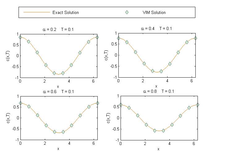
Figure 1: Plots of the exact solution $c(x,t)$, Eq. (41), and the truncated VIM solution $c_{7}(x,t)$, Eq. (4.1), at $t=0.1$ and $0\leq x\leq 2\pi$. The plots corresponds $\alpha=$ $0.2,0.4,0.6$ and $0.8$, as indicated.

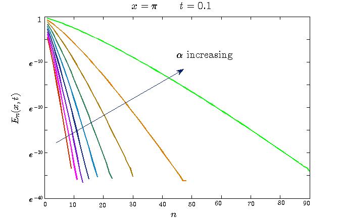
Figure 2: Plot of the relative error $E_{n}(x,t)$ at $x=\pi$, at $t=0.1$ against the number of terms n. Vertical axis is scaled as Natural Logarithm, that is, $\ln e^{m}$, where $m\in\{-40,-35,\cdots,0\}$.

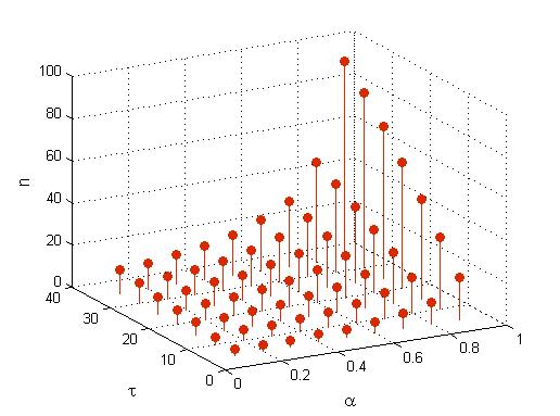
Figure 3: Stem plot for the Table 1. Plot depicts an increase in the values of $n$ as $\alpha$ increases and tolerance level becomes smaller.

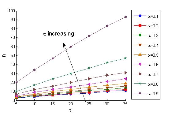
Figure 4: Plots of $n$ against $\tau$, for specific values of $\alpha$.

$\tau$	$\alpha$
	$0.1$	$0.2$	$0.3$	$0.4$	$0.5$	$0.6$	$0.7$	$0.8$	$0.9$
$5$	$3$	$3$	$3$	$4$	$4$	$5$	$7$	$10$	$20$
$10$	$4$	$5$	$5$	$6$	$7$	$9$	$12$	$17$	$34$
$15$	$6$	$6$	$7$	$8$	$10$	$12$	$16$	$24$	$47$
$20$	$7$	$8$	$9$	$10$	$12$	$15$	$20$	$30$	$60$
$25$	$8$	$9$	$11$	$12$	$15$	$18$	$24$	$36$	$72$
$30$	$10$	$11$	$12$	$14$	$17$	$21$	$28$	$42$	$83$
$35$	$11$	$12$	$14$	$16$	$19$	$24$	$31$	$47$	$93$

Table 1: For different values of $\alpha$ and different tolerance levels $\ln e^{-\tau}$, the $n$th approximate solution has to be used to achieve the required accuracy.

4.1 The sinusoidal uploading

Consider the following fractional differential equation

$$\frac{\partial{c(x,t)}}{\partial{t}}={}^{C}_{0}\mathcal{D}_{t}^{\alpha}\left[\frac{\partial^{2}c(x,t)}{\partial x^{2}}\right]+t\sin x,\quad x>0,t>0,$$ (36)

with the initial condition $c(x,0)=\cos x$. On comparing with Eq. (1), we find that the linear operator is $A=\frac{\partial^{2}}{\partial x^{2}}$, the initial data is $f(x)=\cos x$, and the source term is $q(x,t)=t\sin x$, which on comparing with Eq. (26) yields $q_{0}(x)=0$, $q_{1}(x)=\sin x$ and $q_{k}(x)=0$ for $k\geq 2$.

We have following,

$$(A^{n+1}f)(x)=(-1)^{n+1}\cos x,$$ (37)

and

$$(A^{n}q_{1})(x)=(-1)^{n}\sin x.$$ (38)

Substituting Eqs. (37)-(38) in Eq. (3.2), we obtain

$$e_{n+1}(x,t) =(-1)^{n+1}\cos x\frac{t^{(n+1)(1-\alpha)}}{\Gamma[1+(n+1)(1-\alpha)]}$$

$$+(-1)^{n}\sin x\frac{t^{2+n(1-\alpha)}}{\Gamma[3+n(1-\alpha)]}.$$ (39)

Substituting Eq. (4.1) in Eq. (35), we obtain

$$c_{n+1}(x,t) =\cos x\left[1+\sum_{j=0}^{n}(-1)^{j+1}\frac{t^{(j+1)(1-\alpha)}}{\Gamma[1+(j+1)(1-\alpha)]}\right]$$

$$+t^{2}\sin x\left[\sum_{j=0}^{n}(-1)^{j}\frac{t^{j(1-\alpha)}}{\Gamma[j(1-\alpha)+3]}\right].$$ (40)

Taking the limit $n\rightarrow\infty$, we obtain the exact solution,

$$c(x,t)=E_{1-\alpha}[-t^{1-\alpha}]\cos x+t^{2}E_{1-\alpha,3}[-t^{1-\alpha}]\sin x.$$ (41)

Remark: Taking $\alpha=0$, Eq. (36) reduces to conventional partial differential equation,

$$\frac{\partial{c(x,t)}}{\partial{t}}=\frac{\partial^{2}c(x,t)}{\partial x^{2}}+t\sin x,\quad x>0,t>0.$$ (42)

The solution of Eq. (42) can be obtained by putting $\alpha=0$ in Eq. (41), that gives,

$$c(x,t)=E_{1}[-t^{1}]\cos x+t^{2}E_{1,3}[-t^{1}]\sin x,$$ (43)

which agrees with the exact solution

$$c(x,t)=\exp(-t)\cos x+[\exp(-t)+t-1]\sin x.$$ (44)

Figure 1 shows the plots of the exact solution (41) and the VIM approximate solution (4.1) $c_{7}(x,t)$, i.e the truncated sum with $n=6$. The graph shows close agreement between the exact and the VIM solutions. Later, we will present error analysis, that is, error arises when using truncated series as an approximate solution to the exact solution.

4.2 Error Analysis

Our next goal is to investigate the convergence of the approximate solutions obtained by the VIM, Eq. (4.1). For this purpose, we define the relative error as follows,

$$E_{n}(x,t)=\frac{|c(x,t)-c_{n}(x,t)|}{|c(x,t)|}.$$ (45)

Figure 2 shows the plots of relative error at the point $(x,t)=(\pi,0.1)$ against the numer of term $n$ in the truncated VIM solution, for different cases of $\alpha=0.2,0.4,0.6,0.8$. The vertical axis is scaled as Natural Logarithm. The relative errors decay exponentially fast with $n$, but with convergence rates (slope of the plots in Figure 3) that decrease as $\alpha$ approaches 1. Thus, a higher order approximate solution is required to achieve a given level of accuracy as $\alpha$ increases.

Table 1 summaries the results. It show the number of terms $n$ needed for a given for a given accuracy, definded as $e^{-\tau}$, and for different $\alpha$, and . We have depicted the information from Table 1 as a stem plot in Fig. 3, which shows the trends in the number of terms $n$ against $\alpha$ and $\tau$. $n$ increases for all $\alpha$ and $\tau$, but especially sharply as $\alpha$ approaches 1 and the tolerance becomes very small. Moreover, $n$ increases almost linearly with respect to tolerance level $\tau$ for a fixed value of $\alpha$, as shown in Fig. 4.

5 Conclusions:

We have presented solutions of the time fractional diffusion equation with source term

$$\frac{\partial}{\partial t}c(x,t)={}^{C}_{0}\mathcal{D}_{t}^{\alpha}[(Ac)(x,t)]+q(x,t).$$

The solutions are found by using variational iteration method and are presented in the form that avoids the repetition of calculations. The general form of the solutions, obtained by VIM, is expressed in such a way so that it can be implemented on the computer with no difficulty. Validation of the numerical procedure is done for a problem whose exact solution is known. Results obtained by VIM are in agreement with the exact solution. It is shown that only few successive approximations lead to a very good estimate of the exact solution. The truncation errors decay exponentially fast as $n$ increases. VIM proves to be very efficient and fast in finding the solutions of fractional differential equations.

Acknowledgements

The authors would like to acknowledge the support provided by King Abdulaziz City for Science and Technology (KACST) through the Science Technology Unit at King Fahd University of Petroleum and Minerals (KFUPM) for funding this work through project No. 11-OIL1663-04. as part of the National Science, Technology and Innovation Plan (NSTIP).

References

References

• [1] Agrawal, S., Srivastava, M., & Das, S. Synchronization of fractional order chaotic systems using active control method. Chaos, Solitons & Fractals, 45 (2012), 737–752.
• [2] Chen, X., Wang, L., The variational iteration method for solving a neutral functional-differential equation with proportional delays. Computers & Mathematics with Applications, 59 (2010), 2696–2702.
• [3] Das, S. 2011 Functional fractional calculus. Publisher, Springer.
• [4] Elsaid, A. 2010 The variational iteration method for solving riesz fractional partial differential equations. Computers & Mathematics with Applications, 60 (2010), 1940–1947.
• [5] He, J.H. Approximate analytical solution for seepage flow with fractional derivatives in porous media. Computer Methods in Applied Mechanics and Engineering, 167 (1998), 57–68.
• [6] He, J.H. Variational iteration method–a kind of non-linear analytical technique: some examples. International journal of non-linear mechanics, 34 (1999), 699–708.
• [7] Hilfer, R. Fractional time evolution. Applications of fractional calculus in physics , (2000), 87–130.
• [8] Hilfer, R. Applications and implications of fractional dynamics for dielectric relaxation, in: Recent Advances in Broadband Dielectric Spectroscopy, pp. 123–130. Pub. Springer, 2013.
• [9] Kilbas, A.A., Srivastava, H.M., & Trujillo, J.J. Theory and Applications of Fractional differential equations. Pub, North-Holland Mathematics Studies, Elsevier, 2006.
• [10] Luchko, Y. & Punzi, A. Modeling anomalous heat transport in geothermal reservoirs via fractional diffusion equations. GEM-International Journal on Geomathematics, 1 (2011), 257–276.
• [11] Magin, R.& Ovadia, M. Modeling the cardiac tissue electrode interface using fractional calculus. J. Vibration and Control, 14 (2008), 1431–1442.
• [12] Magin, R.L. Fractional calculus models of complex dynamics in biological tissues. Computers & Mathematics with Applications, 59 (2010), 1586–1593.
• [13] Mainardi, F. An historical perspective on fractional calculus in linear viscoelasticity. Fractional Calculus and Applied Analysis, 15 (2012), 712–717.
• [14] Metzler, R. & Klafter, J. The random walk’s guide to anomalous diffusion: a fractional dynamics approach. Physics reports, 339 (2000), 1–77.
• [15] Metzler, R. & Klafter, J. The restaurant at the end of the random walk: recent developments in the description of anomalous transport by fractional dynamics. J. Physics A: Mathematical and General, 37 (2004), R161.
• [16] MolliqΒ R, Y., Noorani, M. & Hashim, I. Variational iteration method for fractional heat-and wave-like equations. Nonlinear Analysis: Real World Applications, 10 (2009), 1854–1869.
• [17] Momani, S. & Odibat, Z. Comparison between the homotopy perturbation method and the variational iteration method for linear fractional partial differential equations. Computers & Mathematics with Applications, 54 (2007), 910–919.
• [18] Noor, M.A. & Mohyud-Din, S.T. Variational iteration method for unsteady flow of gas through a porous medium using heΓ’TMs polynomials and pade approximants. Computers & Mathematics with Applications, 58 (2009), 2182–2189.
• [19] Noor, M.A. & Mohyud-Din, S.T. Variational iteration method for solving twelfth-order boundary-value problems using heΓ’TMs polynomials. Computational Mathematics and Modeling, 21 (2010), 239–251
• [20] Odibat, Z. & Momani, S. Application of variational iteration method to nonlinear differential equations of fractional order. International Journal of Nonlinear Sciences and Numerical Simulation, 7 (2006), 27–34.
• [21] Ross, B. Fractional calculus and its applications Proceedings of the international conference held at the University of New Haven, June, 1974. Volume 457. Pub. Springer.
• [22] Sakar, M.G., Erdogan, F. & YΔ±ldΔ±rΔ±m, A. Variational iteration method for the time-fractional fornberg–whitham equation. Computers & Mathematics with Applications, 73 (2012), 1382–1388
• [23] Sandev, T., Metzler, R. & Tomovski, Ε½. Fractional diffusion equation with a generalized riemann–liouville time fractional derivative. J. Physics A: Mathematical and Theoretical, 44 (2011), 255203.
• [24] Scalas, E., Gorenflo, R. & Mainardi, F. Fractional calculus and continuous-time finance. Physica A: Statistical Mechanics and its Applications, 284 (2000), 376–384.
• [25] Shirazian, M. & Effati, S. Solving a class of nonlinear optimal control problems via heΓ’TMs variational iteration method. International Journal of Control, Automation and Systems, 10 (2012), 249–256.
• [26] Wazwaz, A.M. Partial differential equations and solitary waves theory. Pub. Springer, 2009.