On Integration Methods Based on Scrambled Nets of Arbitrary Size

Abstract

We consider the problem of evaluating $I(\varphi):=\int_{[0,1)^{s}}\varphi(\mathbf{x})\mathrm{d}\mathbf{x}$ for a function $\varphi\in L^{2}[0,1)^{s}$. In situations where $I(\varphi)$ can be approximated by an estimate of the form $N^{-1}\sum_{n=0}^{N-1}\varphi(\mathbf{x}^{n})$, with $\{\mathbf{x}^{n}\}_{n=0}^{N-1}$ a point set in $[0,1)^{s}$, it is now well known that the $\mathcal{O}_{P}(N^{-1/2})$ Monte Carlo convergence rate can be improved by taking for $\{\mathbf{x}^{n}\}_{n=0}^{N-1}$ the first $N=\lambda b^{m}$ points, $\lambda\in\{1,\dots,b-1\}$, of a scrambled $(t,s)$-sequence in base $b\geq 2$. In this paper we derive a bound for the variance of scrambled net quadrature rules which is of order ${\scriptscriptstyle\mathcal{O}}(N^{-1})$ without any restriction on $N$. As a corollary, this bound allows us to provide simple conditions to get, for any pattern of $N$, an integration error of size ${\scriptscriptstyle\mathcal{O}}_{P}(N^{-1/2})$ for functions that depend on the quadrature size $N$. Notably, we establish that sequential quasi-Monte Carlo (M. Gerber and N. Chopin, 2015, J. R. Statist. Soc. B, 77 (3), 509-579) reaches the ${\scriptscriptstyle\mathcal{O}}_{P}(N^{-1/2})$ convergence rate for any values of $N$. In a numerical study, we show that for scrambled net quadrature rules we can relax the constraint on $N$ without any loss of efficiency when the integrand $\varphi$ is a discontinuous function while, for sequential quasi-Monte Carlo, taking $N=\lambda b^{m}$ may only provide moderate gains.

1 Introduction

We consider the problem of evaluating $I(\varphi):=\int_{[0,1)^{s}}\varphi(\mathbf{x})\mathrm{d}\mathbf{x}$ for a function $\varphi\in L^{2}[0,1)^{s}$. Focussing first on unweighed quadrature rules of the form $I(P^{N},\varphi)=N^{-1}\sum_{n=0}^{N-1}\varphi(\mathbf{x}^{n})$, with $P^{N}=\{\mathbf{x}^{n}\}_{n=0}^{N-1}$ a set of $N$ points in $[0,1)^{s}$, the simplest way to approximate $I(\varphi)$ is to use the Monte Carlo estimator which selects for $P^{N}$ a set of $N$ independent uniform random variates on $[0,1)^{s}$. The central limit theorem then ensures that the variance of the approximation error $I(P^{N},\varphi)-I(\varphi)$ is of order $\mathcal{O}(N^{-1})$. However, it is now well known that this rate can be improved by taking for $P^{N}$ a randomized quasi-Monte Carlo (RQMC) point set. In particular, Owen (1995) proposes a randomization scheme for $(t,s)$-sequences in base $b\geq 2$, known as nested scrambling, such that the variance of the quadrature rule $I(P^{N},\varphi)$ decreases faster than $N^{-1}$ when $P^{N}$ is the set made of the first $N$ points of the resulting randomized sequence (Owen, 1997a, 1998). Owen (1997a, 1998) also establishes that, in this case, $\mathrm{Var}(I(P^{N},\varphi))\leq c_{t}N^{-1}\sigma^{2}$ for a constant $c_{t}<\infty$ independent of $\varphi$ and where $N^{-1}\sigma^{2}=N^{-1}\int_{[0,1)^{s}}(\varphi(\mathbf{x})-I(\varphi))^{2}\mathrm{d}\mathbf{x}$ is the variance of a Monte Carlo quadrature rule of the same size. Interestingly, Owen (1997a) shows that the constant $c_{0}$ has the additional property to be independent of the dimension $s$.

In some complicated settings, the function $\varphi$ cannot be computed explicitly and/or the dimension $s$ is too large for a simple unweighted quadrature rule $I(P^{N},\varphi)$ to be efficient. Important examples where such a problem arises are parameter and state inference in state space models. Recently, Gerber and Chopin (2015) have developed a sequential quasi-Monte Carlo (SQMC) algorithm to carry out sequential inference in this class of models. When this algorithm uses points taken from scrambled $(t,s)$-sequences as inputs, it outperforms Monte Carlo methods with an error of size ${\scriptscriptstyle\mathcal{O}}_{P}(N^{-1/2})$ for continuous and bounded functions (Gerber and Chopin, 2015, Theorem 7).

However, all these results apply only for $N=\lambda b^{m}$, $\lambda\in\{1,\dots,b-1\}$. This restriction on the values of $N$ arises because the approximation error of the aforementioned integration methods depends on the equidistribution properties of the scrambled nets at hand and, as we go through a scrambled $(t,s)$-sequences in base $b$, sets with the strongest equidistribution properties are constituted of $b^{m}$ consecutive points, $m\geq t$ (see Section 2 for a review on $(t,s)$-sequences). From a practical point of view, this means that a (large) variance reduction can only be obtained at the price of a sharply increasing running time, which may reduce the attractiveness of scrambled net integration methods when one is interested, e.g., to reach a given level of precision at the lowest computational effort.

The objective of this paper is to study quadrature rules and SQMC based on scrambled nets of arbitrary size. Our main theoretical contribution is to provide a bound for the variance of the scrambled net quadrature rule $I(P^{N},\varphi)$ which shows that the ${\scriptscriptstyle\mathcal{O}}(N^{-1})$ convergence rate obtained by Owen (1997a, 1998) under the restriction $N=\lambda b^{m}$ in fact holds for any pattern $N$. This bound also provides conditions to have an error of size ${\scriptscriptstyle\mathcal{O}}_{P}(N^{-1/2})$ for the integral of a function $\varphi_{N}$ which depends on the quadrature size $N$, as it typically happens in sequential estimation methods. A consequence of this last result is the asymptotic superiority of SQMC over sequential Monte Carlo algorithms without any restriction on $N$. Relaxing the constraint $N=b^{m}$ is particularly important for SQMC because in many applications (such as, e.g., target tracking) inference in state space models should be carried in real time and, consequently, it may be too costly to double the number of simulations in order to reduce the variance (assuming $b=2$). Having a free control of $N$ is also crucial for parameter inference in state space models if, e.g., one wants to use SQMC as a sampling strategy inside particle Markov Chain Monte Carlo methods (Andrieu et al., 2010). Indeed, efficient allocations of the computational budget between the time spent to run the filtering algorithm and the length of the Markov chain require a fine control of $N$ as explained, e.g., in Doucet et al. (2013).

In addition to a variance of order ${\scriptscriptstyle\mathcal{O}}(N^{-1})$, we show two interesting properties of scrambled net quadrature rules of arbitrary size. First, when points of a scrambled $(0,s)$-sequence are used, the variance of the quadrature rule admits a bound of the form $c^{*}_{0}\sigma^{2}N^{-1}$ for an explicit constant $c^{*}_{0}>0$ which is independent of the integrand $\varphi$ and of the dimension $s$. Second, Yue and Mao (1999, Theorem 4) establish that for smooth integrands the integration error of quadratures based on scrambled sequences is of order $\mathcal{O}_{P}(N^{-1}(\log N)^{(s-1)/2})$. We note in this work that for such functions the error is in fact of size $\mathcal{O}_{P}(N^{-1})$. In a recent paper, Owen (2014) has shown that this rate is the best we can achieve uniformly in $N$ for equally weighted quadrature rules and therefore, on this class of functions, quadratures based on scrambled sequences have the optimal worst case behaviour.

The rest of this paper is organized as follows. Section 2 gives the notation and the background material used in this work. The announced results for quadrature rules $I(P^{N},\varphi)$ based on scrambled nets are formally stated in Section 3. In Section 4 we provide conditions to get the ${\scriptscriptstyle\mathcal{O}}_{P}(N^{-1/2})$ convergence rate for integrands that depend on $N$ and discuss the application of this result in the context of SQMC. To simplify the presentation, we propose in this section a convergence result for a scrambled net version of the sampling importance resampling (SIR) algorithm introduced by Rubin (1987, 1988) rather than for SQMC. This SIR algorithm based on scrambled nets is sequentially used in SQMC and the steps to prove its error rate are exactly the same as the ones needed to relax the constrain on $N$ in Gerber and Chopin (2015, Theorem 7). In Section 5 the question of the impact of $N$ on the convergence rate for both scrambled nets quadrature rules and for SQMC is analysed in a numerical study while Section 6 concludes.

2 Background

In this section we provide the background material on $(t,s)$-sequences, scrambled sequences and on the Haar-like decomposition of $L^{2}[0,1)^{s}$ introduced by Owen (1997a). Only the concepts and the results used in this paper are presented. For a complete exposition of these notions we refer the reader, respectively, to Dick and Pillichshammer (2010, Chapter 4), Owen (1995) and Owen (1997a, 1998).

For integers $s\geq 1$ and $b\geq 2$, let

$$\mathcal{E}^{b}=\left\{\prod_{j=1}^{s}\left[a_{j}b^{-d_{j}},(a_{j}+1)b^{-d_{j}}\right)\subseteq[0,1)^{s},\,a_{j},\,d_{j}\in\mathbb{N},\,a_{j}<b^{d_{j}},\,j=1,...,s\right\}$$

be the set of all $b$-ary boxes.

Let $t$ and $m$ be two positive integers such that $m\geq t$. Then, the point set $\{\mathbf{x}^{n}\}_{n=0}^{b^{m}-1}$ is called a $(t,m,s)$-net in base $b$ if every $b$-ary box of volume $b^{t-m}$ contains exactly $b^{t}$ points, while the point set $\{\mathbf{x}^{n}\}_{n=0}^{\lambda b^{m}-1}$, $\lambda\in\{1,\dots,b-1\}$, is called a $(\lambda,t,m,s)$-net if every $b$-ary box of volume $b^{t-m}$ contains exactly $\lambda b^{t}$ points and no $b$-ary box of volume $b^{t-m-1}$ contains more than $b^{t}$ points. A sequence $(\mathbf{x}^{n})_{n\geq 0}$ of points in $[0,1)^{s}$ is called a $(t,s)$-sequence in base $b\geq 2$ if, for any integers $a\geq 0$ and $m\geq t$, the point set $\{\mathbf{x}^{n}\}_{n=ab^{m}}^{(a+1)b^{m}-1}$ is a $(t,m,s)$-net in base $b$. Finally, note that if $(\mathbf{x}^{n})_{n\geq 0}$ is a $(t,s)$-sequence in base $b$, then, for $\lambda\in\{1,\dots,b-1\}$, $\{\mathbf{x}^{n}\}_{n=ab^{m+1}}^{ab^{m+1}+\lambda b^{m}-1}$ is a $(\lambda,t,m,s)$-net for any integers $a\geq 0$ and $m\geq t$.

To introduce the Haar-like decomposition of $L^{2}[0,1)^{s}$ developed by Owen (1997a), let $u\subseteq\mathcal{S}:=\{1,...,s\}$, $\kappa$ be a vector of $|u|$ non negative integers $k_{(u,j)}$, $j\in\{1,\dots,|u|\}$, $|\kappa|=\sum_{j=1}^{|u|}k_{(u,j)}$, and

$$\mathcal{E}^{b}_{u,\kappa}=\left\{\prod_{j=1}^{s}\left[a_{j}b^{-d_{j}},(a_{j}+1)b^{-d_{j}}\right)\in\mathcal{E}^{b}:\,d_{j}=k_{(u,j)}+1\text{ if }j\in u\text{ and }d_{j}=0\text{ if }j\notin u\right\}.$$

Then, Owen (1997a) shows that $\varphi(\mathbf{x})=\sum_{u\subseteq\mathcal{S}}\sum_{\kappa}\nu_{u,\kappa}(\mathbf{x})$ where, for any $u\subseteq\mathcal{S}$, we use the shorthand $\sum_{\kappa}=\sum_{k_{(u,1)}=0}^{\infty}\dots\sum_{k_{(u,|u|)}=0}^{\infty}$ and $\nu_{u,\kappa}$ is a step function, constant over each of the $b^{|u|+|\kappa|}$ sets $E\in\mathcal{E}^{b}_{u,\kappa}$ and which integrates to zero over any $b$-ary box that strictly contains a set $E\in\mathcal{E}^{b}_{u,\kappa}$. These step functions are mutually orthogonal and $\nu_{\varnothing,()}$ is constant over $[0,1)^{s}$. The resulting ANOVA decomposition of $\varphi$ is given by

$$\sigma^{2}=\sum_{|u|>0}\sum_{\kappa}\sigma_{u,\kappa}^{2}$$ (1)

with $\sigma_{u,\kappa}^{2}=\int_{[0,1)^{s}}\nu_{u,\kappa}^{2}(\mathbf{x})\mathrm{d}\mathbf{x}$.

Let $P^{N}=\{\mathbf{x}^{n}\}_{n=0}^{N-1}$, $\mathbf{x}^{n}=(x_{1}^{n},\dots,x_{s}^{n})$, be the first $N\geq 1$ points of a $(t,s)$-sequence in base $b\geq 2$ where, for $j\in\mathcal{S}$, $x_{j}^{n}=\sum_{i=1}^{\infty}a_{jni}b^{-i}$ with $a_{jni}\in\{0,\dots,b-1\}$ for all $n$ and $i$. Owen (1995) proposes a method to randomly permute the digits $a_{jnk}$ such that the scrambled point set $\tilde{P}^{N}=\{\tilde{\mathbf{x}}^{n}\}_{n=0}^{N-1}$ preserves almost surely the equidistribuion properties of the original net $P^{N}$. In addition, under this randomization scheme, each $\tilde{\mathbf{x}}^{n}$ is marginally uniformly distributed on $[0,1)^{s}$ and Owen (1997a) shows that

$$\mathrm{Var}\left(I(\tilde{P}^{N},\varphi)\right)=\frac{1}{N}\sum_{|u|>0}\sum_{\kappa}\Gamma_{u,\kappa}\sigma^{2}_{u,\kappa}$$ (2)

where $\Gamma_{u,\kappa}$ depends on the properties of the non scrambled point set $\{\mathbf{x}^{n}\}_{n=0}^{N-1}$. In particular, for an arbitrary value of $N\in\mathbb{N}^{*}$, the gain factors $\Gamma_{u,\kappa}$ are bounded by (Hickernell and Yue, 2001, Lemma 11)

$$\Gamma_{u,\kappa}\leq b^{t+1}\left(\frac{b+1}{b-1}\right)^{s+1}.$$ (3)

When the point set $P^{N}$ is a $(\lambda,t,m,s)$-net, the gain factors can be more precisely controlled. Notably, Owen (1998, Lemma 2) obtains

$$\mathrm{Var}\left(I(\tilde{P}^{N},\varphi)\right)=\frac{1}{N}\sum_{|u|>0}\sum_{|\kappa|>m-t-|u|}\Gamma_{u,\kappa}\sigma^{2}_{u,\kappa}$$ (4)

where $\Gamma_{u,\kappa}\leq\Gamma^{(b)}_{t,s}$ with $\Gamma^{(b)}_{0,s}=e$ if $b\geq s$ (Owen, 1997b, Theorem 1; Hickernell and Yue, 2001, Lemma 6) and, for $t>0$, $\Gamma^{(b)}_{t,s}=b^{t}(b+1)^{s}/(b-1)^{s}$ (Owen, 1998, Lemma 4). Together with equation Eq. (4), these bounds for the gain factors imply that

$$\mathrm{Var}\left(I(\tilde{P}^{N},\varphi)\right)={\scriptscriptstyle\mathcal{O}}(N^{-1}),\quad\mathrm{Var}\left(I(\tilde{P}^{N},\varphi)\right)\leq\Gamma^{(b)}_{t,s}\frac{\sigma^{2}}{N}$$ (5)

where we recall that $\tilde{P}^{N}$ contains the first $N=\lambda b^{m}$ points of a scrambled $(t,s)$-sequence in base $b\geq 2$.

We conclude this section by noting that all the results presented in this work also hold for the computationally cheaper scrambling method proposed by Matoǔsek (1998), although in what follows we will only refer to the scrambling technique developed by Owen (1995) for ease of presentation. In addition, even if it is not always explicitly mentioned, all the scrambled nets we consider in this paper are made of the first $N$ points of a scrambled $(t,s)$-sequence.

3 Quadratures based on scrambled nets of arbitrary size

3.1 Error bounds

A first result concerning the error bound of quadratures based on scrambled nets of an arbitrary size $N\geq 1$ can be directly deduced from Eq. (2) and Eq. (3). Indeed, if $\tilde{P}^{N}$ contains the first $N\in\mathbb{N}^{*}$ points of a scrambled $(t,s)$-sequence in base $b\geq 2$, these two bounds imply that

$$\mathrm{Var}\left(I(\tilde{P}^{N},\varphi)\right)\leq\frac{\sigma^{2}}{N}b^{t+1}\left(\frac{b+1}{b-1}\right)^{s+1}=\Gamma^{(b)}_{t+1,s+1}\frac{\sigma^{2}}{N}$$ (6)

so that the variance of a scrambled net quadrature is never larger than a constant times the Monte Carlo variance. However, this bound is larger than the one in Eq. (5) obtained under the restriction $N=\lambda b^{m}$ because the equidistribution properties of $\tilde{P}^{N}$ are the strongest when $N$ satisfies this constraints.

The following theorem is the main result of this work and provides a sharper bound (for $N$ large enough) for the integration error (see A.1 for a proof).

Theorem 1.

Let $\varphi\in L^{2}[0,1)^{s}$, $\sigma^{2}=\int_{[0,1)^{s}}\varphi^{2}(\mathbf{x})\mathrm{d}\mathbf{x}-\big{(}\int_{[0,1)^{s}}\varphi(\mathbf{x})\mathrm{d}\mathbf{x}\big{)}^{2}$ and $\tilde{P}^{N}=\{\tilde{\mathbf{x}}^{n}\}_{n=0}^{N-1}$ be the first $N\in\mathbb{N}^{*}$ points of a $(t,s)$-sequence in base $b\geq 2$ scrambled as in Owen (1995). Let $N\geq 1$ and $k\in\mathbb{N}$ be such that $b^{k}\leq N<b^{k+1}$. Then,

$$\mathrm{Var}\big{(}I(\tilde{P}^{N},\varphi)\big{)} \leq 2\frac{\Gamma_{t,s}^{(b)}}{N}\bigg{\{}(1+c_{b})B^{(k)}_{t}+c_{b}\Big{[}B^{(k)}_{t+1}+\sum_{|u|>0}b^{-\frac{k-1-t-|u|}{2}}\sum_{|\kappa|\leq k-1-t-|u|}\,b^{\frac{|\kappa|}{2}}\sigma_{u,\kappa}^{2}\Big{]}\bigg{\}}$$

$$+b^{2t}\frac{\sigma^{2}}{N^{2}}$$

where $c_{b}=\frac{(b-1)^{1/2}}{b^{1/2}-1}$,

$$B^{(k)}_{c}=\sum_{|u|>0}\,\sum_{|\kappa|>k-c-|u|}\sigma_{u,\kappa}^{2}+\sum_{|u|>0}b^{-(k-c-|u|)}\sum_{|\kappa|\leq k-c-|u|}\sigma_{u,\kappa}^{2}b^{|\kappa|},\quad c\in\mathbb{N}$$

and where we use the convention that empty sums are null.

The bound provided in Theorem 1 is hard to interpret but its main purpose is to study the rate at which the variance goes to zero as the quadrature size increases. Thanks to Kronecker’s lemma, we show in Corollary 1 below that this theorem implies that for any square integrable function the error is of size ${\scriptscriptstyle\mathcal{O}}_{P}(N^{-1/2})$ without any restriction on $N$. Due to its importance for this work, Kronecker’s lemma is recalled in Lemma 2 below (see, e.g., Shiryaev, 1996, Lemma 2, p.390, for a proof).

Lemma 2 (Kronecker’s Lemma).

Let $(d_{n})_{n\geq 1}$ be a sequence of positive increasing numbers such that $d_{n}\rightarrow\infty$ as $n\rightarrow\infty$, and let $(z_{n})_{n\geq 1}$ be a sequence of numbers such that $\sum_{n=1}^{\infty}z_{n}$ converges. Then, as $N\rightarrow\infty$, $d^{-1}_{N}\sum_{n=1}^{N}d_{n}z_{n}\rightarrow 0$.

If the expression of the bound given Theorem 1 is rather complicated, we note from the proof of this result that the variance of quadratures based on points taken from scrambled $(0,s)$-sequences is never larger than a universal constant $c_{0}^{*}$ times the Monte Carlo variance. In addition, for $t>0$, we derive from the proof of this theorem a simple bound for the variance which is in most cases sharper than the one given in Eq. (6). These results are collected in the following corollary.

Corollary 1.

Consider the set-up of Theorem 1. Then,

$$\mathrm{Var}\big{(}I(\tilde{P}^{N},\varphi)\big{)}={\scriptscriptstyle\mathcal{O}}(N^{-1}).$$

In addition,

$$\mathrm{Var}\big{(}I(\tilde{P}^{N},\varphi)\big{)} \leq\frac{\sigma^{2}}{N}\bigg{\{}\Big{[}\Gamma_{t,s}^{(b)}(1+2c_{b})\Big{]}^{1/2}+\frac{b^{t}}{N^{1/2}}\bigg{\}}^{2}$$ (7)

and, for $t=0$,

$$\mathrm{Var}\big{(}I(\tilde{P}^{N},\varphi)\big{)}\leq\frac{\sigma^{2}}{N}e\,(3+2\sqrt{2})<15.85\frac{\sigma^{2}}{N}.$$ (8)

Proof.

To prove the error rate, let $\tilde{\sigma}_{u,l}^{2}=\sum_{\kappa:|\kappa|=l}\sigma_{u,\kappa}^{2}$ for $l\in\mathbb{N}$ and note that, for any fixed integers $a>0$, $0\leq c<k-s$ and $u\subseteq\mathcal{S}$,

$$b^{-a(k-c-|u|)}\sum_{|\kappa|\leq k-c-|u|}\sigma_{u,\kappa}^{2}b^{a|\kappa|} =b^{-a(k-c-|u|)}\sum_{l=0}^{k-c-|u|}b^{al}\,\tilde{\sigma}_{u,l}^{2}=b^{-a(k-c-|u|+1)}\sum_{l=1}^{k-c-|u|+1}b^{al}\,\tilde{\sigma}_{u,l-1}^{2}$$

which converges to zero by Kronecker’s lemma. Also, because $\sum_{|u|>0}\sum_{\kappa}\sigma_{u,\kappa}^{2}=\sigma^{2}$, this shows that, as $N\rightarrow\infty$, $B^{(k)}_{t}\rightarrow 0$ and $B_{t+1}^{(k)}\rightarrow 0$ and therefore, using Theorem 1, as $N\rightarrow\infty$, $N\mathrm{Var}\big{(}I(\tilde{P}^{N},\varphi)\big{)}\rightarrow 0$. The proof of the bounds given in Eq. (7)-Eq. (8) is postponed to A.2. ∎

When $N\leq b^{t}$, the trivial bound $\mathrm{Var}\big{(}I(\tilde{P}^{N},\varphi)\big{)}\leq\sigma^{2}$ is sharper than the bounds given in Eq. (6) and in Eq. (7). To compare these latter when $N>b^{t}$, note that, for all $b\geq 2$, $(1+2c_{b})<b(b+1)/(b-1)$. Thus, the bound in Eq. (7) is sharper that the one provided in Eq. (6) for any $N>b^{t}N_{s}^{(b)}$ with

$$N_{s}^{(b)}=\bigg{\{}\bigg{(}\frac{b+1}{b-1}\bigg{)}^{s}\bigg{[}\bigg{(}b\frac{b+1}{b-1}\bigg{)}^{1/2}-(1+2c_{b})^{1/2}\bigg{]}^{2}\bigg{\}}^{-1}.$$ (9)

Simple computations show that $N_{s}^{(b)}$ decreases as $b\geq 2$ and/or $s\geq 1$ increases and, for $b\geq 5$, $N_{s}^{(b)}<1$ for all $s\geq 2$.

Table 1 below gives the value of $\max(1,N_{s}^{(b)})$ for different prime numbers $b\geq 2$ and for dimension $s>b$ so that a $(0,s)$-sequence in base $b$ does not exist (see Dick and Pillichshammer, 2010, Corollary 4.36, p.141); that is, for values of $s$ such that the bound given in Eq. (8) cannot apply. As one may expect, remark that the bound in Eq. (7) is larger than the one given in Eq. (5) for quadratures based on $(\lambda,t,m,s)$-nets.

$s$	3	4	5	6	7	$>8$
$\max(1,N_{s}^{(2)})$	29.77	9.93	3.31	1.11	1	1
$\max(1,N_{s}^{(3)})$	-	1.05	1	1	1	1
$\max(N_{s}^{(5)},1)$	-	-	-	1	1	1
$\max(N_{s}^{(>7)},1)$	-	-	-	-	-	1

Table 1: Value of $\max(N_{s}^{(b)},1)$ for different prime numbers $b\geq 2$ and for $s>b$, with $N_{s}^{(b)}$ defined in Eq. (9).

Finally it is worth mentioning that the ${\scriptscriptstyle\mathcal{O}}_{P}(N^{-1/2})$ convergence rate for quadratures based on scrambled nets of arbitrary size was simultaneously established by Art B. Owen (personal communication) using a more direct proof. Nevertheless, the bound given in Theorem 1 also allows to study situations where the integrand depends on the size of the quadrature rule $N$, as explained in Section 4.

3.2 Error rate for smooth integrands

In a recent paper, Owen (2014, Theorem 2) established that the best possible rate for the variance we can have uniformly on $N$ is $N^{-2}$. In this subsection we show that, under some smoothness assumptions on $\varphi$, this optimal rate is achieved by scrambled net quadrature rules in the sense that there exist constants $\underline{c}<\bar{c}<\infty$ such that, for $N$ large enough,

$$\underline{c}<N^{2}\mathrm{Var}\left(I(\tilde{P}^{N},\varphi)\right)<\bar{c}.$$

More precisely, we focus on functions $\varphi\in L_{2}[0,1)^{s}$ such that $\sigma_{u,\kappa}^{2}=\mathcal{O}(b^{-2|\kappa|})$ for all $u\subseteq\mathcal{S}$. Note that this condition is fulfilled when, e.g., $\varphi$ has continuous mixed partial derivative of order $s$ (Owen, 2008, Lemma 2) or when $\varphi$ satisfies the generalized Lipschitz condition considered in Yue and Mao (1999).

For such integrands $\varphi$, simple computations yield the following result:

Proposition 1.

Consider the set-up of Theorem 1 and assume that $\sigma_{u,\kappa}^{2}=\mathcal{O}(b^{-2|\kappa|})$ for all $u\subseteq\mathcal{S}$. Then,

$$\mathrm{Var}\left(I(\tilde{P}^{N},\varphi)\right)=\mathcal{O}(N^{-2}).$$

Proof of Proposition 1..

First, note that under the assumption of the proposition, Owen (1998, Theorem 2) and Owen (2008, Theorem 3) show that, for $m\geq t+s-1$,

$$\sum_{|u|>0}\,\sum_{|\kappa|>m-t-|u|}\sigma_{u,\kappa}^{2}=\mathcal{O}(b^{-2m}m^{s-1}).$$ (10)

Then, let $N\geq b^{t+s-1}$ and $k$ be the largest integer such that $N\geq b^{k}$. The standard way to analyse the variance of a scrambled net quadrature rule of arbitrary size is to decompose $\tilde{P}^{N}$ into scrambled $(a_{m},t,m,s)$-nets $\tilde{P}_{m}$, $m=t,\dots,k$, and a remaining set $\tilde{P}$ that contains $\tilde{n}<b^{t}$ points (see the proof of Theorem 1 for more details). Let $\tilde{P}^{\prime}=\tilde{P}\cup_{m=t}^{t+s-2}\tilde{P}_{m}$. Then, using trivial inequalities and the convention that empty sums are null, we have

$$\mathrm{Var}\bigg{(}I(\tilde{P}^{N},\varphi)\bigg{)}\leq\frac{1}{N^{2}}\bigg{(}\Big{\{}\mathrm{Var}\Big{(}\sum_{\tilde{\mathbf{x}}^{n}\in\tilde{P}^{\prime}}\varphi(\tilde{\mathbf{x}}^{n})\Big{)}\Big{\}}^{1/2}+\sum_{m=t+s-1}^{k}\Big{\{}\mathrm{Var}\Big{(}\sum_{\tilde{\mathbf{x}}^{n}\in\tilde{P}_{m}}\varphi(\tilde{\mathbf{x}}^{n})\Big{)}\Big{\}}^{1/2}\bigg{)}^{2}.$$

Let $\tilde{I}\subset\{0,\dots,N-1\}$ be such that $n\in\tilde{I}$ if and only if $\tilde{\mathbf{x}}^{n}\in\tilde{P}$. Then,

$$\mathrm{Var}\Big{(}\sum_{\tilde{\mathbf{x}}^{n}\in\tilde{P}^{\prime}}\varphi(\tilde{\mathbf{x}}^{n})\Big{)}\leq\Big{(}\sum_{n\in\tilde{I}}\Big{\{}\mathrm{Var}\Big{(}\varphi(\tilde{\mathbf{x}}^{n})\Big{)}\Big{\}}^{1/2}\Big{)}^{2}=|\tilde{P}^{\prime}|^{2}\sigma^{2}<(b^{t+s-1})^{2}\sigma^{2}.$$

In addition, using Eq. (4) and Eq. (10),

$$\sum_{m=t+s-1}^{k}\Big{\{}\mathrm{Var}\Big{(}\sum_{\tilde{\mathbf{x}}^{n}\in\tilde{P}_{m}}\varphi(\tilde{\mathbf{x}}^{n})\Big{)}\Big{\}}^{1/2} =\mathcal{O}\Big{(}\sum_{m=t+s-1}^{k}b^{-m/2}m^{\frac{s-1}{2}}\Big{)}.$$

To conclude the proof, note that the serie $\sum_{m=t+s-1}^{\infty}b^{-m/2}m^{\frac{s-1}{2}}$ is convergent. ∎

We conclude this subsection with two remarks. First, and as in Owen (1998, Theorem 2), the computations in the proof of Proposition 1 hold for $N\geq b^{t+s}$ and thus we cannot expect that the variance decreases as $N^{-2}$ for smaller quadrature sizes. Second, the rate of order $\mathcal{O}_{P}(N^{-2}(\log N)^{s-1})$ found by Yue and Mao (1999), under the same assumptions as in Proposition 1, is due to the fact that, in the last step of the proof of this latter, they use the inequality $\sum_{m=t+s-1}^{k}b^{-m/2}m^{(s-1)/{2}}<k^{(s-1)/{2}}(1-b^{-1/2})^{-1}$ rather than using the fact that the series $\sum_{m=t+s-1}^{\infty}b^{-m/2}m^{(s-1)/{2}}$ is convergent.

4 Error rate for integrands that depend on the quadrature size

We now analyse the behaviour of the quadrature $I(\tilde{P}^{N},\varphi_{N})$ where $(\varphi_{N})_{N\geq 1}$ is a sequence of real valued functions. In practice, the sequence of functions $(\varphi_{N})_{N\geq 1}$ is often such that, as $N\rightarrow\infty$, $\varphi_{N}\rightarrow\varphi$ where $I(\varphi)$ is the quantity of interest. The classical situation where this set-up occurs is when we are estimating $I(\varphi)$ using a sequential method such as the array-RQMC algorithm developed by L’Ecuyer et al. (2006) or the SQMC algorithm proposed by Gerber and Chopin (2015).

Using Theorem 1, we can deduce the following result concerning the error size of the quadrature rule $I(\tilde{P}^{N},\varphi_{N})$.

Corollary 2.

Consider the set-up of Theorem 1. Let $(\varphi_{N})_{N\geq 1}$ be a sequence of functions such that, $\forall N\in\mathbb{N}^{*}$, $\varphi_{N}\in L^{2}[0,1)^{s}$, and for $N\geq 1$, let

$$\sigma_{N}^{2}=\int_{[0,1)^{s}}\Big{(}\varphi_{N}(\mathbf{x})-\int_{[0,1)^{s}}\varphi_{N}(\mathbf{v})\mathrm{d}\mathbf{v}\Big{)}^{2}\mathrm{d}\mathbf{x},\quad\sigma_{N}^{2}=\sum_{|u|>0}\,\sum_{\kappa}\sigma^{2}_{N,u,\kappa}.$$

Assume that, for any $u\subseteq\mathcal{S}$ and for any $\kappa(u)$, we have, as $N\rightarrow\infty$, $\sigma^{2}_{N,u,\kappa}\rightarrow\sigma^{2}_{u,\kappa}$ and $\sigma_{N}^{2}\rightarrow\sigma^{2}<\infty$, where $\sigma^{2}=\sum_{|u|>0}\,\sum_{\kappa}\sigma^{2}_{u,\kappa}$. Then,

$$\mathrm{Var}\big{(}I(\tilde{P}^{N},\varphi_{N})\big{)}={\scriptscriptstyle\mathcal{O}}(N^{-1}).$$

Proof.

Let $k\in\mathbb{N}$ be the largest power of $b$ such that $b^{k}\leq N$. Then, by Theorem 1, to prove the result we first need to show that, for $a\in\{\frac{1}{2},1\}$ and $c\in\{t,t+1\}$, we have

$$\sum_{|u|>0}b^{-a(k-c-|u|)}\sum_{|\kappa|\leq k-c-|u|}\sigma_{N,u,\kappa}^{2}b^{a|\kappa|}={\scriptscriptstyle\mathcal{O}}(1).$$

To establish this result, let $a$ and $c$ be as above, $k\geq t+s+2$, $k^{\prime}=k-c-|u|+1\geq 2$, $\tilde{k}=\lfloor k^{\prime}/2\rfloor\geq 1$ and $S_{u,p}^{N}=\sum_{l=1}^{p+1}\tilde{\sigma}_{N,u,l-1}^{2}$ where $\tilde{\sigma}^{2}_{N,u,l}$ is defined as in the proof of Corollary 1. Note that the positive and increasing sequence $(S_{u,p}^{N})_{p\geq 1}$ converges to $\sigma_{N,u}^{2}=\sum_{|\kappa|>0}\sigma^{2}_{N,u,\kappa}$ as $p\rightarrow\infty$. Then, using summation by part and similar computations as in the proof of Kronecker’s lemma (see, e.g., Shiryaev, 1996, Lemma 2, p.390), we have

$$b^{-a(k-c-|u|)}\sum_{l=0}^{k-c-|u|}\tilde{\sigma}_{N,u,l}^{2}b^{al} =b^{-ak^{\prime}}\sum_{l=1}^{k^{\prime}}\tilde{\sigma}_{N,u,l-1}^{2}b^{al}$$

$$=S^{N}_{u,k^{\prime}}-b^{-ak^{\prime}}\sum_{l=1}^{\tilde{k}-1}(b^{a(l+1)}-b^{al})S^{N}_{u,l}-b^{-ak^{\prime}}\sum_{l=\tilde{k}}^{k^{\prime}-1}(b^{a(l+1)}-b^{al})\sigma_{N,u}^{2}$$

$$-b^{-ak^{\prime}}\sum_{l=\tilde{k}}^{k^{\prime}-1}(b^{a(l+1)}-b^{al})(S^{N}_{u,l}-\sigma_{N,u}^{2})$$

$$\leq\frac{b^{a\tilde{k}}}{b^{ak^{\prime}}}\sigma_{N,u}^{2}+(\sigma_{N,u}^{2}-S^{N}_{u,\tilde{k}})$$

so that (recall that $\tilde{k}$ and $k^{\prime}$ depend on $|u|$)

$$\sum_{|u|>0}b^{-a(k-c-|u|)}\sum_{|\kappa|\leq k-c-|u|}\sigma_{N,u,\kappa}^{2}b^{a|\kappa|}\leq\sum_{|u|>0}b^{a(\tilde{k}-k^{\prime})}\sigma_{N,u}^{2}+\Big{(}\sigma_{N}^{2}-\sum_{|u|>0}S^{N}_{u,\tilde{k}}\Big{)}.$$ (11)

Then, using Fatou’s Lemma,

$$0\leq\limsup_{k\rightarrow\infty}\Big{(}\sigma_{N}^{2}-\sum_{|u|>0}S^{N}_{u,\tilde{k}}\Big{)} =\limsup_{k\rightarrow\infty}\Big{(}\sigma_{N}^{2}-\sum_{|u|>0}\sum_{l\geq 0}\mathbb{I}(l\leq\tilde{k})\tilde{\sigma}^{2}_{N,u,l}\Big{)}$$

$$\leq\sigma^{2}-\liminf_{k\rightarrow\infty}\sum_{|u|>0}\sum_{l\geq 0}\mathbb{I}(l\leq\tilde{k})\tilde{\sigma}^{2}_{N,u,l}$$

$$\leq\sigma^{2}-\sum_{|u|>0}\sum_{l\geq 0}\liminf_{k\rightarrow\infty}\mathbb{I}(l\leq\tilde{k})\tilde{\sigma}^{2}_{N,u,l}$$

$$=0$$

because each $\tilde{\sigma}^{2}_{N,u,l}$ is a finite sum of some $\sigma^{2}_{N,u,\kappa}$’s and, by assumption, $\sigma^{2}_{N,u,\kappa}\rightarrow\sigma^{2}_{u,\kappa}$ for any $u$ and $\kappa$. This shows that the second term of Eq. (11) converges to zero as $N\rightarrow\infty$. The above computations also show that, for any $u\subseteq\mathcal{S}$, $\sigma^{2}_{N,u}$ converges to $\sum_{|\kappa|>0}\sigma^{2}_{u,\kappa}$ so that $b^{a(\tilde{k}-k^{\prime})}\sigma_{N,u}^{2}\rightarrow 0$ as $N\rightarrow\infty$. Hence, the right-hand side of Eq. (11) goes to zero as $N$ increases, as required. To conclude the proof note that these computations also imply that, as $N\rightarrow\infty$, $\sum_{|u|>0}\sum_{|\kappa|\leq k-c-|u|}\sigma_{N,u,\kappa}^{2}\rightarrow 0$.

∎

4.1 Application of Corollary 2 to SQMC and to sampling importance resampling

A direct consequence of Corollary 2 is to relax the constraint on $N$ in Gerber and Chopin (2015, Theorem 7), showing that on the class of continuous and bounded functions SQMC asymptotically outperforms standard sequential Monte Carlo algorithms without any restriction on how the number of simulations (or “particles”) grows.

Providing a complete description of SQMC is beyond the scope of this work (see however Section 5.2 for an example of SQMC algorithm). Nevertheless, to get some insight about how Corollary 2 applies to this class of methods, we illustrate this result by studying a scrambled net version of the sampling importance resampling (SIR) algorithm proposed by Rubin (1987, 1988), which is iteratively used in SQMC. In addition, and as already mentioned, the steps used to establish the convergence rate of the latter (Proposition 2 below) are exactly the same that those needed to extend Gerber and Chopin (2015, Theorem 7) to an arbitrary pattern of $N$.

SIR algorithms are designed to estimate the expectation $\pi(f):=\int_{[0,1)^{s}}f(\mathbf{x})\pi(\mathbf{x})\mathrm{d}\mathbf{x}$, with $\pi$ a density function on $[0,1)^{s}$; see Algorithm 1 for the pseudo-code version of the proposed QMC version of SIR. In Algorithm 1, $q(\mathbf{x})\mathrm{d}\mathbf{x}$ is a proposal distribution on $[0,1)^{s}$ and, for a probability measure $\mu$ on $[0,1)^{s}$, $\bm{F}^{-1}_{\mu}:[0,1)^{s}\rightarrow[0,1)^{s}$ denotes the (generalized) inverse of $\bm{F}_{\mu}$, the Rosenblatt transformation of $\mu$ (see Rosenblatt, 1952, for a definition). Finally, $h:[0,1]^{s}\rightarrow[0,1]$ is a pseudo-inverse of the Hilbert space filling curve $H:[0,1]\rightarrow[0,1]^{s}$, which is a continuous mapping from the unit interval onto the unit hypercube (see, e.g., Hamilton and Rau-Chaplin, 2008, for how to construct the Hilbert curve for any $s\geq 2$).

Using Corollary 2 and the results in Gerber and Chopin (2015), we can prove that the error of Algorithm 1 to approximate $\pi(f)$ is of size ${\scriptscriptstyle\mathcal{O}}_{P}(N^{-1/2})$ for any pattern of $N$, as shown in the next result.

Algorithm 1 QMC sampling importance resampling

1:Generate $\tilde{P}_{1}^{N}=\{\tilde{\mathbf{x}}_{1}^{n}\}_{n=0}^{N-1}$ a scrambled net in $[0,1)^{s}$ and $\tilde{P}_{2}^{N}=\{\tilde{x}_{2}^{n}\}_{n=0}^{N-1}$ a scrambled net in $[0,1)$

2:Compute $\mathbf{z}_{1}^{n}=\bm{F}_{q}^{-1}(\tilde{\mathbf{x}}_{1}^{n})$ and $w^{n}=\pi(\mathbf{z}_{1}^{n})/q(\mathbf{z}_{1}^{n})$ for $n=0,\dots,N-1$

3:Compute $I(\tilde{P}_{2}^{N},\varphi_{N})$ where $\varphi_{N}=f\circ F_{h,N}^{-1}$ with $F^{-1}_{h,N}$ the (generalized) inverse of the empirical cumulative density function $F_{h,N}(z)=\sum_{n=0}^{N-1}\frac{w^{n}}{\sum_{m=0}^{N-1}w^{m}}\mathbb{I}(h(\mathbf{z}_{1}^{n})\leq z)$

4:return $I(\tilde{P}_{2}^{N},\varphi_{N})$, an estimate of $\pi(f)$

Proposition 2.

Consider Algorithm 1 where $\tilde{P}_{1}$ and $\tilde{P}_{2}$ are independent. Assume that the functions $f(\mathbf{z})$ and $\pi(\mathbf{z})/q(\mathbf{z})$ are continuous and bounded on $[0,1)^{s}$ and that, for all $i\in\mathcal{S}$, the $i$-th component of $\bm{F}_{q}^{-1}$ is continuous on $[0,1)^{i}$. Then, $\varphi_{N}\rightarrow\varphi:=f\circ F^{-1}_{\pi_{h}}$ almost surely, with $\pi_{h}$ the image by $h$ of $\pi$ and with $I(\varphi)=\pi(f)$. In addition,

$$\mathrm{Var}\Big{(}I(\tilde{P}_{2}^{N},\varphi_{N})\Big{)}={\scriptscriptstyle\mathcal{O}}_{P}(N^{-1}),\quad\mathbb{E}|I(\tilde{P}_{2}^{N},\varphi_{N})-\pi(f)|={\scriptscriptstyle\mathcal{O}}_{P}(N^{-1/2}).$$

Proof.

To show that $\varphi_{N}\rightarrow\varphi$ almost surely, note first that, as $N\rightarrow\infty$, $\|F_{h,N}-F_{\pi_{h}}\|_{\infty}\rightarrow 0$ almost surely by Gerber and Chopin (2015, Theorem 1 and Theorem 3) and therefore, for all $x\in[0,1)$, $F_{h,N}^{-1}(x)\rightarrow F^{-1}_{\pi_{h}}(x)$ with probability one (see the proof of Gerber and Chopin, 2015, Theorem 7). Then, $\varphi_{N}\rightarrow\varphi$ because $f$ is continuous.

To show the second part of the proposition, let $\mathcal{F}_{1}^{N}$ be the $\sigma$-algebra generated by $\{\mathbf{z}_{1}^{n}\}_{n=0}^{N-1}$ and note that

$$\mathrm{Var}\Big{(}I(\tilde{P}_{2}^{N},\varphi_{N})\Big{)} =\mathbb{E}\left[\mathrm{Var}\Big{(}I(\tilde{P}_{2}^{N},\varphi_{N})\big{|}\mathcal{F}_{1}^{N}\Big{)}\right]+\mathrm{Var}\left(\mathbb{E}\Big{[}I(\tilde{P}_{2}^{N},\varphi_{N})\big{|}\mathcal{F}_{1}^{N}\Big{]}\right)$$

$$=\mathbb{E}\left[\mathrm{Var}\Big{(}I(\tilde{P}_{2}^{N},\varphi_{N})\big{|}\mathcal{F}_{1}^{N}\Big{)}\right]+\mathrm{Var}\left(\pi_{N}(f)\right)$$ (12)

where $\pi_{N}(f)=\sum_{n=0}^{N-1}w^{n}f(\mathbf{z}_{1}^{n})/(\sum_{m=0}^{N-1}w^{m})$.

The second term after the second equality sign is ${\scriptscriptstyle\mathcal{O}}(N^{-1})$ by Corollary 1 and by Gerber and Chopin (2015, Theorem 2). For the first term, the same computations as in the proof of Gerber and Chopin (2015, Theorem 7) show that the sequence $(\varphi_{N})_{N\geq 1}$ verifies with probability one the assumptions of Corollary 2. Thus, using this latter,

$$\mathrm{Var}\Big{(}I(\tilde{P}_{2}^{N},\varphi_{N})\big{|}\mathcal{F}_{1}^{N}\Big{)}={\scriptscriptstyle\mathcal{O}}(N^{-1}),\quad\text{almost surely}$$

and therefore the first term in Eq. (12) is ${\scriptscriptstyle\mathcal{O}}(N^{-1})$ by the Dominated Convergence theorem. This shows that $\mathrm{Var}\Big{(}I(\tilde{P}_{2}^{N},\varphi_{N})\Big{)}={\scriptscriptstyle\mathcal{O}}(N^{-1})$. Finally, to establish the result for the $L_{1}$-norm, note that

$$\mathbb{E}|I(\tilde{P}_{2}^{N},\varphi_{N})-\pi(f)| \leq\mathbb{E}|I(\tilde{P}_{2}^{N},\varphi_{N})-\pi_{N}(f)|+\mathbb{E}|\pi_{N}(f)-\pi(f)|$$

$$\leq\left\{\mathrm{Var}\Big{(}I(\tilde{P}_{2}^{N},\varphi_{N})\Big{)}\right\}^{1/2}+\mathbb{E}|\pi_{N}(f)-\pi(f)|$$

where the first term after the second inequality sign is ${\scriptscriptstyle\mathcal{O}}(N^{-1/2})$ from the above computations while the second term is ${\scriptscriptstyle\mathcal{O}}(N^{-1/2})$ by Corollary 1 and by Gerber and Chopin (2015, Theorem 2). ∎

5 Numerical Study

In this section we illustrate the main findings of this paper. All the simulations presented below rely on a Sobol’ sequence that is scrambled using the method proposed by Owen (1995). We recall that $b=2$ for the Sobol’ sequence.

5.1 Scrambled net quadrature rules

We consider the problem of estimating the $s$-dimensional integral $I(\varphi_{j})$, $j=1,\dots,4$, where

$$\varphi_{1}(\mathbf{x})=\sum_{i=1}^{s}x_{i},\quad\varphi_{2}(\mathbf{x})=\max\Big{(}\sum_{i=1}^{s}x_{i}-\frac{s}{2},0\Big{)},\quad\varphi_{3}(\mathbf{x})=\mathbb{I}_{\left(\sum_{i=1}^{s}x_{i}>\frac{s}{2}\right)}(\mathbf{x})$$

are as in He and Owen (2014) and where $\varphi_{4}(\mathbf{x})=12^{s/2}\prod_{i=1}^{s}(x_{i}-0.5)$ is as in Owen (1997b, 1998). Note that the integrands $\varphi_{1}$ and $\varphi_{2}$ are both Lipschitz continuous but $\varphi_{2}$ is not everywhere differentiable, while $\varphi_{4}$ satisfies the assumption of Proposition 1 (Owen, 1997b). For $j\in\{1,\dots,4\}$, we estimate the integral $I(\varphi_{j})$ using the quadrature rule $I(\tilde{P}^{N},\varphi_{j})$ where, as mentioned above, $\tilde{P}^{N}$ is the set containing the first $N$ points of a scrambled Sobol’ sequence.

Figure 1 shows the evolution of the mean square errors (MSEs) as a function of $N$. Results are presented for $N$ ranging from $1$ to $2^{18}$, with $s=3$ for $\varphi_{j}$, $j=1,2,3$, and $s=6$ for $\varphi_{4}$. In addition to the MSEs, we have reported the Monte Carlo $N^{-1}$ reference line to illustrate the result of Corollary 1, namely that the convergence rate is faster than $N^{-1}$ for any pattern of $N$. To illustrate the finding of Proposition 1, we have also represented a $N^{-2}$ reference line in the plot showing the results for the quadrature $I(\tilde{P}^{N},\varphi_{4})$ (Figure 1(d)). This $N^{-2}$ reference line starts at $N=b^{t+s}=2^{14}$, which is the value of $N$ from which we can naively expect that the quadrature $I(\tilde{P}^{N},\varphi_{4})$ enters in the asymptotic regime (see Section 3.2).

To compare quadrature rules based on nets of arbitrary size with those based on $(t,m,s)$-nets, Figure 1 also shows the evolution of the MSEs along the subsequence $N=2^{m}$. The interesting point to note here is that, for a given value of $s$, the advantage of using $(t,m,s)$-nets over nets of arbitrary size decreases as the integrand becomes “less smooth”. Indeed, for the everywhere differentiable and Lipschitz function $\varphi_{1}$, we observe that taking for $N$ powers of 2 significantly improves the convergence rate. In addition, this choice for the quadrature size $N$ is also the cheapest way to reach any given level of MSE. For the function $\varphi_{2}$ this observation holds for $N\geq 2^{8}$ but the gain in term of convergence rate is smaller than for the estimation of $I(\varphi_{1})$. Finally, the advantage of taking a power of 2 for the quadrature size has completely disappeared for the discontinuous function $\varphi_{3}$.

To understand these observations recall that, by Proposition 1, the (asymptotic) convergence rate of $\mathrm{Var}\big{(}I(\tilde{P}^{N},\varphi)\big{)}$ is $N^{-2}$ uniformly on $N$ when $\varphi$ is smooth enough so that the quantities $\sigma_{u,\kappa}^{2}$’s decrease sufficiently quickly as $|\kappa|$ increases. However, under the conditions of Proposition 1, the error size of quadratures based on scrambled $(t,m,s)$-nets is of order $\mathcal{O}(N^{-3/2}(\log N)^{(s-1)/2}$ (Owen, 2008, Theorem 3) and is thus smaller than what is obtained for an arbitrary value of $N$. More generally, and as illustrated in Figure 1, the error size of quadratures based on scrambled $(\lambda,t,m,s)$-nets depends positively on the smoothness of the integrand (for more theoretical results on this point, see Owen, 1997b, 1998; Yue and Mao, 1999; Hickernell and Yue, 2001). Consequently, taking $N=b^{k}$ is the best choice for the smooth integrands $\varphi_{1}$ and $\varphi_{2}$ since then the MSE goes to zero much faster than $N^{-2}$. Note that for $\varphi_{2}$ the MSE obtained by taking $N=2^{k}$ decreases slower than for $\varphi_{1}$ and, as a result, $N$ should be larger to rule out the choice $N\neq b^{k}$. Finally, for the discontinuous function $\varphi_{3}$ the convergence rate of the MSE when using $(t,m,s)$-nets is too slow for the choice of $N$ to influence that of the MSE.

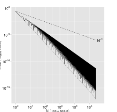
(a)

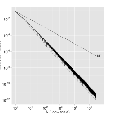
(b)

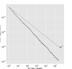
(c)

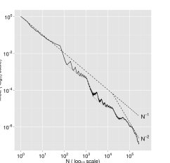
(d)

Figure 1: Mean square error of $I(\tilde{P}^{N},\varphi_{1})$ (Figure 1(a)), $I(\tilde{P}^{N},\varphi_{2})$ (Figure 1(b)), $I(\tilde{P}^{N},\varphi_{3})$ (Figure 1(c)) and $I(\tilde{P}^{N},\varphi_{4})$ where $\tilde{P}^{N}$ contains the first $N$ points of a scrambled Sobol’ sequence. The dotted lines present the results along the subsequence $N=2^{m}$ for $m=0,\dots,18$ and the solid lines the MSEs for any $N\in\{1,\dots 2^{16}\}$. In Figure 1(d), the $N^{-2}$ reference line starts at $N=b^{t+s}=2^{14}$. The results are obtained from 1 000 independent repetitions.

5.2 Likelihood function estimation in state space models

We now study the problem of estimating the likelihood function of the following generic univariate state space model

$$\begin{cases}y_{k}|z_{k}\sim\mathcal{N}\left(\mu_{y}(z_{k}),\sigma_{y}^{2}(z_{k})\right),&k\geq 0\\ z_{k}|z_{k-1}\sim\mathcal{N}\left(\mu_{z}(z_{k-1}),\sigma_{z}^{2}(z_{k-1})\right),&k\geq 1\\ z_{0}\sim\mathcal{N}(\mu_{0},\sigma_{0}^{2})\end{cases}$$ (13)

where $(y_{k})_{k\geq 0}$ is the observation process, $(z_{k})_{k\geq 0}$ is the hidden Markov process and where $\mu_{q}:\mathbb{R}\rightarrow\mathbb{R}$ and $\sigma_{q}:\mathbb{R}\rightarrow\mathbb{R}^{+}$, $q\in\{z,y\}$, are known functions.

Given a set of $T\geq 1$ observations $\{y_{k}\}_{k=0}^{T-1}$, we denote by $p(y_{0:T-1})$ the likelihood function of the model defined by (13), which cannot be computed explicitly. Indeed, writing $f(\cdot{},\mu,\sigma^{2})$ the density function of the $\mathcal{N}(\mu,\sigma^{2})$ distribution, it is easy to see that (using the convention that $f\big{(}z_{k},\mu_{z}(z_{k-1}),\sigma^{2}_{z}(z_{k-1})\big{)}=f\big{(}z_{0},\mu_{0},\sigma_{0}^{2}\big{)}$ when $k=0$)

$$p(y_{0:T-1})=\int_{\mathbb{R}^{T}}\prod_{k=0}^{T-1}f\big{(}y_{k},\mu_{y}(z_{k}),\sigma_{y}^{2}(z_{k})\big{)}f\big{(}z_{k},\mu_{z}(z_{k-1}),\sigma^{2}_{z}(z_{k-1})\big{)}\mathrm{d}z_{k}$$ (14)

where, in practical scenarios, the time horizon $T$ is large (at least several dozen). In addition, simple unweighed quadrature rules are generally very inefficient to evaluate the integral appearing in Eq. (14). To see this, note that $p(y_{0:T-1})=I(\varphi_{T})$ where $\varphi_{T}:[0,1)^{T}\rightarrow\mathbb{R}$ is given by

$$\varphi_{T}(x_{0},\dots,x_{T-1})=\tilde{\varphi}_{T}\circ F^{-1}_{T}(x_{0},\dots,x_{T-1})$$

with $\tilde{\varphi}_{T}(z_{0},\dots,z_{T-1})=\prod_{k=0}^{T-1}f(y_{k},\mu_{y}(z_{k}),\sigma^{2}_{y}(z_{k}))$ and $F_{T}$ the Rosenblatt transformation of the probability measure on $\mathbb{R}^{T}$ defined by

$$\prod_{k=0}^{T-1}f\big{(}z_{k},\mu_{z}(z_{k-1}),\sigma_{z}^{2}(z_{k-1})\big{)}\mathrm{d}z_{k}.$$

Because $T$ is typically large, the function $\varphi_{T}$ is concentrated in a tiny region of the integration domain and, consequently, quadrature rules require a huge number of points to provide a precise estimate of $p(y_{0:T-1})$. An efficient way to get an (unbiased) estimate $p^{N}(y_{0:T-1})$ of $p(y_{0:T-1})$ is to use a SQMC algorithm (Gerber and Chopin, 2015); that is, a QMC version of sequential Monte Carlo methods which are standard tools to handle this kind of problems (see, e.g., Doucet et al., 2001). The suitable SQMC algorithm for the generic state space model (13) is presented in Algorithm 2, where we use the standard notation $\Phi(\cdot)$ for the cumulative density function (CDF) of the $\mathcal{N}(0,1)$ distribution. Note that inference in state space model (13) is just an example of problems that can be addressed using SQMC and, in particular, SQMC is not restricted to Gaussian models.

To see the connection between the results presented in Sections 3-4 and Algorithm 2, note that the likelihood function $p(y_{0:T-1})$ can be decomposed as follows:

$$p(y_{0:T-1})=\prod_{k=0}^{T-1}p(y_{k}|y_{0},\dots,y_{k-1})$$

with the convention that $p(y_{k}|y_{0},\dots,y_{k-1})=p(y_{0})$ when $k=0$. Then, Algorithm 2 amounts to recursively computing an approximation of the form $N^{-1}\sum_{n=1}^{N}w_{k}^{n}=I(\varphi_{N,k},\tilde{P}_{k}^{N})$ of the incremental likelihood $p(y_{k}|y_{0},\dots,y_{k-1})$, $k=0,\dots,T-1$.

At iteration $k=0$, $\varphi_{N,k}$ is the function $f(y_{0},\mu_{y}(\cdot),\sigma_{y}^{2}(\cdot))$ which therefore does not depend on $N$. Thus, iteration 0 of Algorithm 2 is a simple scramble net quadrature rule which enters in the framework of Section 3. For $k\geq 1$, it is easy to see that

$$\varphi_{N,k}(\mathbf{x})=f\left(y_{k},\mu_{y}\circ g(\mathbf{x}),\sigma^{2}_{y}\circ g(\mathbf{x})\right),\quad g(\mathbf{x})=\mu_{z}\circ F_{N,k-1}^{-1}(x_{1})+\sigma_{z}\circ F_{N,k-1}^{-1}(x_{1})\Phi^{-1}(x_{2})$$

and thus, for $k\geq 1$, we are in the set-up of Section 4 where the integrand depends on the quadrature size $N$.

Algorithm 2 SQMC Algorithm to estimate $p(y_{0:T-1})$ in the state space model (13)

1:Generate a RQMC point set $\tilde{P}^{N}_{0}=\{\tilde{x}_{0}^{n}\}_{n=0}^{N-1}$ in $[0,1)$

2:Compute $z_{0}^{n}=\mu_{0}+\sigma_{0}\Phi^{-1}(\tilde{x}_{0}^{n})$ and $w_{0}^{n}=f\left(y_{0},\mu_{y}(z_{0}^{n}),\sigma^{2}_{y}(z_{0}^{n})\right)$, $n=0,\dots,N-1$

3:Normalize the weights: $W_{0}^{n}=w_{0}^{n}/\sum_{m=0}^{N-1}w_{0}^{m}$, $n=0,\dots,N-1$

4:Compute $p^{N}(y_{0})=N^{-1}\sum_{n=0}^{N-1}w_{0}^{n}$

5:for $k=1\rightarrow T-1$ do

6:      Generate a RQMC point set $\tilde{P}_{k}^{N}=\{\tilde{\mathbf{x}}^{n}_{k}\}_{n=0}^{N-1}$ in $[0,1)^{2}$; let $\tilde{\mathbf{x}}_{k}^{n}=(\tilde{x}_{k}^{n},\tilde{v}^{n}_{k})$

7:     for $n=0\rightarrow N-1$ do

8:          Compute $\tilde{z}_{k-1}^{n}=F_{N,k-1}^{-1}(\tilde{x}_{k}^{n})$ where $F_{N,k-1}(z)=\sum_{m=0}^{N-1}W_{k-1}^{m}\mathbb{I}(z^{m}_{k-1}\leq z)$

9:         Compute $z_{k}^{n}=\mu_{z}(\tilde{z}_{k-1}^{n})+\sigma_{z}(\tilde{z}_{k-1}^{n})\Phi^{-1}(\tilde{v}_{k}^{n})$

10:         Compute $w_{k}^{n}=f\left(y_{k},\mu_{y}(z_{k}^{n}),\sigma^{2}_{y}(z_{k}^{n})\right)$

11:     end for

12:     Normalize the weights: $W_{k}^{n}=w_{k}^{n}/\sum_{m=0}^{N-1}w_{k}^{m}$, $n=0,\dots,N-1$

13:     Compute $p^{N}(y_{0:k})=p^{N}(y_{0:k-1})\,N^{-1}\sum_{n=0}^{N-1}w_{k}^{n}$

14:end for

15:return $p^{N}(y_{0:T-1})$, an estimate of $p(y_{0:T-1})$

In this simulation study we analyse the MSE of $\log p^{N}(y_{0:T-1})$ when at Step 1 and at Step 6 of Algorithm 2 the RQMC point sets are the first $N$ points of independent scrambled Sobol’ sequences, where $N=4i$ for $i=3,\dots,2^{11}$. Note that, since the function $F_{N,k-1}^{-1}$ in the definition of $\varphi_{N,k}$ is discontinuous, the results of the previous subsection suggest that the gain of restricting $N$ to be powers of the Sobol’ sequence can only be moderate in the context of SQMC. In addition, it is worth remarking that this gain will also depend on the regularity of the functions $\mu_{q}$ and $\sigma_{q}$, $q\in\{y,z\}$.

5.2.1 Stochastic volatility (SV) model

We first consider the following simple univariate SV model

$$\begin{cases}y_{k}|z_{k}\sim\mathcal{N}\left(0,e^{-0.1+z_{k}}\right),&k\geq 0\\ z_{k}|z_{k-1}\sim\mathcal{N}\left(0.9z_{k-1},0.1\right),&k\geq 1\\ z_{0}\sim\mathcal{N}(0,\frac{0.1}{1-0.9^{2}})\end{cases}$$ (15)

from which a set of 100 observations is generated. Figure 2(a) presents the MSE of the estimator $\log p^{N}(y_{0:T-1})$ as well as the $N^{-1}$ Monte Carlo reference line. As expected from the results of Section 4, we see that the ${\scriptscriptstyle\mathcal{O}}_{P}(N^{-1})$ convergence rate for the SQMC algorithm holds uniformly on $N$. Nevertheless, we observe in this example that selecting $N=2^{m}$ is optimal as soon as $N\geq 2^{9}$ in the sense that this choice guarantees the smallest MSE for a given computational budget.

Interestingly, despite the discontinuities of the integrand we are facing at iteration $k\geq 1$ of SQMC, these first results look like those obtained for $\varphi_{2}$ in Section 5.1 rather than like the ones we obtained for the discontinuous mapping $\varphi_{3}$. A possible explanation for this apparent contradiction is that the only source of discontinuities comes from the function $F_{N,k-1}^{-1}$. However, as $N$ increases, we can expect that the empirical CDF of the particles generated at time $k\geq 0$ (and its inverse) converges to a continuous function since all the random variables have a continuous distribution. Under some conditions we can show that this is indeed the case (see, e.g., Proposition 2 above or the proof of Theorem 7 in Gerber and Chopin, 2015). In addition, the SV model (15) is an example of state space model (13) where the functions $\mu_{q}$ and $\sigma^{2}_{q}$, $q\in\{y,z\}$, are very smooth.

5.2.2 A non-linear and non-stationary model

We now consider the following non-linear and non-stationary well known toy example in the particle filtering literature (see, e.g., Gordon et al., 1993)

$$\begin{cases}y_{k}|z_{k}\sim\mathcal{N}\left(\frac{z_{k}^{2}}{20},1\right),&k\geq 0\\ z_{k}|z_{k-1}\sim\mathcal{N}\left(0.5z_{k-1}+25\frac{z_{k-1}}{1+z_{k-1}^{2}}+8\cos(1.2k),10\right),&k\geq 1\\ z_{0}\sim\mathcal{N}(0,2)\end{cases}$$ (16)

from which we again simulate a set of 100 observations. Note that, in addition to the non-linearity of $\mu_{z}$, the density of the law of $y_{k}|x_{k}$ is bimodal when $y_{k}>0$. Due to these additional difficulties, we therefore expect that the gain of restricting $N$ to be a power of 2 is less profitable than for the SV model. This point is confirmed in the Figure 2(b) where we show the evolution of the MSE as a function of $N$. We indeed remark from this plot that there is no gain of using a number of particles which is a power of two for the values of $N$ considered is this numerical study. However, and as for the SV model, we observe that SQMC converges faster the $N^{-1/2}$ Monte Carlo error rate.

To conclude this section it is worth mentioning that to keep the presentation of SQMC simple we have only shown simulations for univariate models. In the multivariate version of SQMC, the resampling step of Algorithm 2 (Step 8) requires to sort the particles along a Hilbert space filling curve, as in Step 3 of the scrambled net SIR algorithm (Algorithm 1). Since the Hilbert curve is $(1/d)$-Hölder continuous, with $d$ the dimension of the state variable, the estimation problem becomes less smooth as $d$ increases. In light of the observations of this simulation study, this suggests that the gain of restricting $N$ to be powers of the base of the underlying $(t,s)$-sequence is smaller than for univariate models. This point was confirmed in non reported simulation study conducted for the bivariate version of the SV model (15), where the gain of using $(t,m,s)$-nets as input of SQMC has completely disappeared.

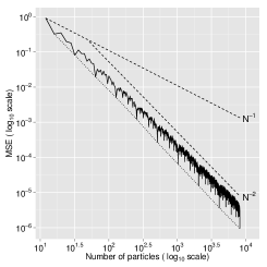
(a)

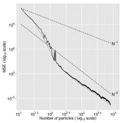
(b)

Figure 2: Mean square errors for the estimation of $\log p(y_{0:T-1})$ in the SV model (15) (Figure 2(a)) and in the toy example (16) (Figure 2(b)). The dotted lines present the results for SQMC for $N=2^{m}$, $m=3,\dots,13$, while the solid lines are for SQMC with $N=4i$, $i=3,\dots,2^{11}$. The results are obtained from 700 independent runs of Algorithm 2.

6 Conclusion

Together with the works of Yue and Mao (1999) and Hickernell and Yue (2001), the present analysis concludes to show that the results of Owen (1997a, b, 1998) obtained for quadrature rules based on $(\lambda,t,s,m)$-nets are in fact true for quadrature rules based on the first $N$ points of scrambled $(t,s)$-sequences without any restriction on the pattern of $N$, namely, to sum-up:

1. For any square integrable functions the integration error goes to zero faster than for the classical Monte Carlo estimator;

2. For any square integrable functions the variance of scrambled quadrature rules is bounded by the Monte Carlo variance multiplied by a constant independent of the integrand;

3. The constant in 2. is uniform with respect to the dimension for scrambled $(0,s)$-sequences;

4. For smooth integrands an explicit convergence rate (better than $N^{-1/2}$) can be computed (see Yue and Mao, 1999; Hickernell and Yue, 2001).

In a simulation study, we show that quadratures based on scrambled $(\lambda,t,m,s)$-nets outperform those based on nets of arbitrary size when the integrand $\varphi$ of interest is smooth. More precisely, using scrambled $(\lambda,t,m,s)$-nets is for such functions the fastest way to reach any given level of MSE. Nevertheless, as the integrand becomes less smooth, this gain decreases and completely disappears for discontinuous functions.

The second important result proved in this paper is the asymptotic superiority of the sequential quasi-Monte Carlo algorithm proposed by Gerber and Chopin (2015) over standard sequential Monte Carlo methods without any restriction on how the number of particles grows. Since SQMC involves integration of discontinuous functions the behaviour of the MSE when the algorithm takes scrambled $(\lambda,t,m,s)$-nets as inputs should not be too different compared to what we would get when scrambled nets of arbitrary size are used. This point is illustrated in a simulation study based in two univariate state space models and we argue that for multivariate models it is very unlikely to expect any gain of using as input for SQMC only points of scrambled sequences that form $(\lambda,t,m,s)$-nets.

Appendix A Proofs

A.1 Proof of Theorem 1

We first prove the following lemma that plays a key role in the proof of Theorem 1.

Lemma 3.

Let $b>1$ (not necessary an integer), $k$ and $t$ be two integers such that $k\geq t\geq 0$ and $v_{m}\in[0,b-1]$, $m=0,...,k$. Then,

$$\sum_{m=t}^{k}v_{m}b^{m}\sum_{|u|>0}\,\sum_{|\kappa|>m-t-|u|}\sigma_{u,\kappa}^{2}\leq\sum_{m=t}^{k}v_{m}b^{m}\sum_{|u|>0}\sum_{|\kappa|>k-t-|u|}\sigma^{2}_{u,\kappa}\\ +b^{k}\sum_{|u|>0}\frac{1}{b^{k-t-|u|}}\sum_{|\kappa|\leq k-t-|u|}\sigma_{u,\kappa}^{2}b^{|\kappa|}$$ (17)

where we use the convention that empty sums are null.

Proof.

For $u\subseteq\mathcal{S}$ and for $l\in\mathbb{Z}$, let $\tilde{\sigma}^{2}_{u,l}=\sum_{\kappa:|\kappa|=l}\sigma^{2}_{u,\kappa}$ if $l\geq 0$ and $\tilde{\sigma}^{2}_{u,l}=0$ otherwise. To simplify the notations, let $k_{t}=k-t$ and $v_{m}^{\prime}=v_{m+t}$. Then,

$$\sum_{m=t}^{k}v_{m}b^{m}\sum_{|u|>0}\,\sum_{|\kappa|>m-t-|u|}\sigma_{u,\kappa}^{2}=b^{t}\sum_{m=0}^{k_{t}}v^{\prime}_{m}b^{m}\sum_{|u|>0}\,\sum_{l>m-|u|}\tilde{\sigma}_{u,l}^{2}.$$

Let $N_{t}=\sum_{m=t}^{k}v_{m}b^{m}$ so that, using Eq. (1), we have

$$\sum_{m=t}^{k}v_{m}b^{m}\sum_{|u|>0}\,\sum_{|\kappa|>m-t-|u|}\sigma_{u,\kappa}^{2}=N_{t}\sigma^{2}-b^{t}\sum_{m=0}^{k_{t}}v^{\prime}_{m}b^{m}\sum_{|u|>0}\,\sum_{l\leq m-|u|}\tilde{\sigma}_{u,l}^{2}.$$ (18)

In order to study the second term of Eq. (18), let $u\subseteq\mathcal{S}$ be such that $k_{t}\geq|u|$. Then,

$$\sum_{m=0}^{k_{t}}v^{\prime}_{m}b^{m}\sum_{l\leq m-|u|}\tilde{\sigma}_{u,l}^{2} =\sum_{m=|u|}^{k_{t}}v^{\prime}_{m}b^{m}\,\sum_{l=0}^{m-|u|}\tilde{\sigma}_{u,l}^{2}=\sum_{m=0}^{k_{t}-|u|}v^{\prime}_{m+|u|}b^{m+|u|}\,\sum_{l=0}^{m}\tilde{\sigma}_{u,l}^{2}.$$

Since

$$\sum_{m=0}^{k_{t}-|u|}v^{\prime}_{m+|u|}b^{m+|u|}\,\sum_{l=0}^{m}\tilde{\sigma}^{2}_{u,l}=\sum_{l=0}^{k_{t}-|u|}\tilde{\sigma}_{u,l}^{2}\,\sum_{m=l}^{k_{t}-|u|}v^{\prime}_{m+|u|}b^{m+|u|},$$

with $b^{t}\sum_{m=l}^{k_{t}-|u|}v^{\prime}_{m+|u|}b^{m+|u|}=N_{t}-\sum_{m=0}^{l+t+|u|-1}v_{m}b^{m}$, we obtain

$$b^{t}\sum_{m=0}^{k_{t}}v^{\prime}_{m}b^{m}\sum_{l=0}^{m-|u|}\tilde{\sigma}_{u,l}^{2} =\sum_{l=0}^{k_{t}-|u|}\Big{(}N_{t}-\sum_{m=0}^{l+t+|u|-1}v_{m}b^{m}\Big{)}\tilde{\sigma}_{u,l}^{2}.$$

Therefore, using Eq. (18) and the convention that empty sums are null,

$$\sum_{m=t}^{k}v_{m}b^{m}\sum_{|u|>0}\,\sum_{|\kappa|>m-t-|u|}\sigma_{u,\kappa}^{2} =N_{t}\sigma^{2}-\sum_{|u|>0}\,\sum_{l=0}^{k_{t}-|u|}\Big{(}N_{t}-\sum_{m=0}^{l+t+|u|-1}v_{m}b^{m}\Big{)}\tilde{\sigma}_{u,l}^{2}$$

$$=N_{t}\sum_{|u|>0}\,\sum_{l>k_{t}-|u|}\tilde{\sigma}^{2}_{u,l}+\sum_{|u|>0}\sum_{l=0}^{k_{t}-|u|}\tilde{\sigma}_{u,l}^{2}\sum_{m=0}^{l+t+|u|-1}v_{m}b^{m}.$$

Finally, since $v_{m}\leq b-1$, we have, for $u\subseteq\mathcal{S}$ such that $k_{t}\geq|u|$,

$$\sum_{l=0}^{k_{t}-|u|}\tilde{\sigma}_{u,l}^{2}\sum_{m=0}^{l+|u|+t-1}v_{m}b^{m} \leq(b-1)\sum_{l=0}^{k_{t}-|u|}\tilde{\sigma}_{u,l}^{2}\frac{b^{l+|u|+t}-1}{b-1}\leq b^{k}\Big{(}\frac{1}{b^{k-t-|u|}}\sum_{l=0}^{k_{t}-|u|}\tilde{\sigma}_{u,l}^{2}b^{l}\Big{)}.$$

This shows that

$$\sum_{m=t}^{k}v_{m}b^{m}\sum_{|u|>0}\,\sum_{|\kappa|>m-t-|u|}\sigma_{u,\kappa}^{2}\leq\sum_{m=t}^{k}v_{m}b^{m}\sum_{|u|>0}\sum_{|\kappa|>k-t-|u|}\sigma^{2}_{u,\kappa}\\ +b^{k}\sum_{|u|>0}\frac{1}{b^{k-t-|u|}}\sum_{l\leq k-t-|u|}\tilde{\sigma}_{u,l}^{2}b^{l}$$

and the proof of the lemma is complete.

∎

To prove Theorem 1, and following the proof of Niederreiter (1992, Lemma 4.11, p.56), we decompose $\{\tilde{\mathbf{x}}^{n}\}_{n=0}^{N-1}$, $N\geq 1$, into scrambled $(\lambda_{m},t,m,s)$-nets $\tilde{P}_{m}$, $m=t,\dots,k$, and a remaining set $\tilde{P}$ that contains strictly less than $b^{t}$ points. We recall that $k$ is the largest power of $b$ such that $b^{k}\leq N$.

To construct this partition of $\{\tilde{\mathbf{x}}^{n}\}_{n=0}^{N-1}$, let $N=\sum_{m=0}^{k}a_{m}b^{m}$ be the expansion of $N$ in base $b\geq 2$, with $a_{m}\in\{0,...,b-1\}$ and $a_{k}\neq 0$. Then, let $\tilde{P}_{k}=\{\tilde{\mathbf{x}}^{n}\}_{n=0}^{a_{k}b^{k}-1}$ and, for $0\leq m\leq k-1$, let $\tilde{P}_{m}$ be the point set made of the $\tilde{\mathbf{x}}^{n}$’s with $\sum_{h=m+1}^{k}a_{h}b^{h}\leq n<\sum_{h=m}^{k}a_{h}b^{h}$. By definition of a $(t,s)$-sequence, $\tilde{P}_{m}$ is a scrambled $(a_{m},t,m,s)$-nets in base $b\geq 2$ for $m=t,\dots,k$ while $\tilde{P}=\cup_{m=0}^{t-1}\tilde{P}_{m}$ has cardinality strictly smaller than $b^{t}$.

Using this decomposition of $\{\tilde{\mathbf{x}}^{n}\}_{n=0}^{N-1}$ we have, using the convention that empty sums are equal to zero,

$$\mathrm{Var}\bigg{(}\frac{1}{N}\sum_{n=0}^{N-1}\varphi(\tilde{\mathbf{x}}^{n})\bigg{)} =\mathrm{Var}\bigg{(}\frac{1}{N}\sum_{\tilde{\mathbf{x}}\in\tilde{P}}\varphi(\tilde{\mathbf{x}})+\frac{1}{N}\sum_{m=t}^{k}\sum_{\tilde{\mathbf{x}}\in\tilde{P}_{m}}\varphi(\tilde{\mathbf{x}})\bigg{)}$$

$$\leq\Bigg{(}\frac{1}{N}\bigg{\{}\mathrm{Var}\Big{(}\sum_{\tilde{\mathbf{x}}\in\tilde{P}}\varphi(\tilde{\mathbf{x}})\Big{)}\bigg{\}}^{1/2}+\frac{1}{N}\sum_{m=t}^{k}\bigg{\{}\mathrm{Var}\Big{(}\sum_{\tilde{\mathbf{x}}\in\tilde{P}_{m}}\varphi(\tilde{\mathbf{x}})\Big{)}\bigg{\}}^{1/2}\Bigg{)}^{2}$$

$$=\frac{1}{N^{2}}\mathrm{Var}\bigg{(}\sum_{\tilde{\mathbf{x}}\in\tilde{P}}\varphi(\tilde{\mathbf{x}})\bigg{)}+\bigg{(}\frac{1}{N}\sum_{m=t}^{k}\bigg{\{}\mathrm{Var}\Big{(}\sum_{\tilde{\mathbf{x}}\in\tilde{P}_{m}}\varphi(\tilde{\mathbf{x}})\Big{)}\bigg{\}}^{1/2}\bigg{)}^{2}$$

$$+\frac{2}{N}\bigg{\{}\mathrm{Var}\Big{(}\sum_{\tilde{\mathbf{x}}\in\tilde{P}}\varphi(\tilde{\mathbf{x}})\Big{)}\bigg{\}}^{1/2}\frac{1}{N}\sum_{m=t}^{k}\bigg{\{}\mathrm{Var}\Big{(}\sum_{\tilde{\mathbf{x}}\in\tilde{P}_{m}}\varphi(\tilde{\mathbf{x}})\Big{)}\bigg{\}}^{1/2}.$$ (19)

To bound the first term of Eq. (19), let $\tilde{J}\subset\{0,\dots,N-1\}$ be such that $n\in\tilde{J}$ if and only if $\tilde{\mathbf{x}}^{n}\in\tilde{P}$. Then, note that

$$\mathrm{Var}\bigg{(}\sum_{\tilde{\mathbf{x}}\in\tilde{P}}\varphi(\tilde{\mathbf{x}})\bigg{)}\leq\bigg{(}\sum_{n\in\tilde{J}}\Big{\{}\mathrm{Var}\big{(}\varphi(\tilde{\mathbf{x}}^{n})\big{)}\Big{\}}^{1/2}\bigg{)}^{2}=|\tilde{P}|^{2}\sigma^{2}<b^{2t}\sigma^{2}$$

and therefore

$$\frac{1}{N^{2}}\mathrm{Var}\bigg{(}\sum_{\tilde{\mathbf{x}}\in\tilde{P}}\varphi(\tilde{\mathbf{x}})\bigg{)}\leq\frac{b^{2t}}{N^{2}}\sigma^{2}.$$ (20)

To bound the second term of Eq. (19) define, for $m\in\{t,\dots,k\}$, $\hat{I}_{m}=(a_{m}b^{m})^{-1}\sum_{\tilde{\mathbf{x}}\in\tilde{P}_{m}}\varphi(\tilde{\mathbf{x}})$ if $m$ is such that $a_{m}\neq 0$ and set $\hat{I}_{m}=0$ otherwise. Then,

$$\bigg{(}\frac{1}{N}\sum_{m=t}^{k}\bigg{\{}\mathrm{Var}\Big{(}\sum_{\tilde{\mathbf{x}}\in\tilde{P}_{m}}\varphi(\tilde{\mathbf{x}})\Big{)}\bigg{\}}^{1/2}\bigg{)}^{2}=\bigg{(}\frac{1}{N}\sum_{m=t}^{k}\bigg{\{}\mathrm{Var}\Big{(}a_{m}b^{m}\hat{I}_{m}\Big{)}\bigg{\}}^{1/2}\bigg{)}^{2}$$

$$=\frac{1}{N^{2}}\sum_{m=t}^{k}\mathrm{Var}(a_{m}b^{m}\hat{I}_{m})+\frac{2}{N^{2}}\sum_{k\geq m>n\geq t}\mathrm{Var}(a_{m}b^{m}\hat{I}_{m})^{1/2}\mathrm{Var}(a_{n}b^{n}\hat{I}_{n})^{1/2}.$$ (21)

Using Eq. (4) we have, for $m$ such that $a_{m}\neq 0$,

$$\mathrm{Var}(\hat{I}_{m})\leq\Gamma^{(b)}_{t,s}(a^{m}b^{m})^{-1}\sum_{|u|>0}\,\sum_{|\kappa|>m-t-|u|}\sigma_{u,\kappa}^{2}$$

and therefore, using Lemma 3 and the fact that $b^{k}\leq N$,

$$\sum_{m=t}^{k}\mathrm{Var}(a_{m}b^{m}\hat{I}_{m})\leq\Gamma^{(b)}_{t,s}\sum_{m=t}^{k}a_{m}b^{m}\sum_{|u|>0}\,\sum_{|\kappa|>m-t-|u|}\sigma_{u,\kappa}^{2}\leq N\,\Gamma^{(b)}_{t,s}\,B^{(k)}_{t}$$

where $B^{(k)}_{t}$ is as in the statement of the theorem. Hence, $N^{-1}\sum_{m=t}^{k}\mathrm{Var}(a_{m}b^{m}\hat{I}_{m})\leq\Gamma^{(b)}_{t,s}B_{t}^{(k)}$.

To study the second term of Eq. (21), let $m>n\geq t$. Then, easy computations show that

$$\frac{(a_{n}a_{m}b^{n+m})^{1/2}}{\Gamma^{(b)}_{t,s}}\mathrm{Var}(\hat{I}_{m})^{1/2}\mathrm{Var}(\hat{I}_{n})^{1/2} \leq\Big{(}\sum_{|u|>0}\,\sum_{|\kappa|>m-t-|u|}\sigma_{u,\kappa}^{2}\Big{)}^{1/2}\Big{(}\sum_{|u|>0}\,\sum_{|\kappa|>n-t-|u|}\sigma_{u,\kappa}^{2}\Big{)}^{1/2}$$

$$\leq\frac{1}{2}\Big{(}\sum_{|u|>0}\,\sum_{|\kappa|>m-t-|u|}\sigma_{u,\kappa}^{2}+\sum_{|u|>0}\,\sum_{|\kappa|>n-t-|u|}\sigma_{u,\kappa}^{2}\Big{)}$$

and therefore

$$\frac{2}{\Gamma^{(b)}_{t,s}}\sum_{m=t+1}^{k}\sum_{n=t}^{m-1}\mathrm{Var}(a_{m}b^{m}\hat{I}_{m})^{1/2}\mathrm{Var}(a_{n}b^{n}\hat{I}_{n})^{1/2}$$

$$=\frac{2}{\Gamma^{(b)}_{t,s}}\sum_{m=t+1}^{k}\sum_{n=t}^{m-1}(a_{m}a_{m})^{1/2}b^{\frac{n+m}{2}}\left\{(a_{m}a_{n}b^{n+m})^{1/2}\big{\{}\mathrm{Var}(\hat{I}_{m})\big{\}}^{1/2}\big{\{}\mathrm{Var}(\hat{I}_{n}))\big{\}}^{1/2}\right\}$$

$$\leq\sum_{m=t+1}^{k}\sum_{n=t}^{m-1}\Big{\{}(a_{m}a_{n})^{1/2}b^{\frac{n+m}{2}}\sum_{|u|>0}\,\sum_{|\kappa|>m-t-|u|}\sigma_{u,\kappa}^{2}+(a_{n}a_{m})^{1/2}b^{\frac{m+n}{2}}\sum_{|u|>0}\,\sum_{|\kappa|>n-t-|u|}\sigma_{u,\kappa}^{2}\Big{\}}.$$

Consequently, since $\sum_{n=t}^{m-1}a_{n}^{1/2}b^{n/2}\leq c_{b}b^{m/2}$, with $c_{b}=\sqrt{b-1}/(b^{1/2}-1)$, we have

$$\frac{2}{\Gamma^{(b)}_{t,s}}\sum_{m=t+1}^{k}\sum_{n=t}^{m-1}\mathrm{Var}(a_{m}b^{m}\hat{I}_{m})^{1/2} \mathrm{Var}(a_{n}b^{n}\hat{I}_{n})^{1/2}\leq c_{b}\Big{(}\sum_{m=t+1}^{k}a_{m}b^{m}\sum_{|u|>0}\,\sum_{|\kappa|>m-t-|u|}\sigma_{u,\kappa}^{2}\Big{)}$$

$$+\sum_{m=t+1}^{k}a_{m}^{1/2}b^{m/2}\Big{(}\sum_{n=t}^{m-1}a_{n}^{1/2}b^{n/2}\sum_{|u|>0}\,\sum_{|\kappa|>n-t-|u|}\sigma_{u,\kappa}^{2}\Big{)}$$ (22)

where, by Lemma 3, the first term in bracket is bounded by $NB^{(k)}_{t}$. For the second term in bracket, we have, using Lemma 3 (where $k$ is replaced by $m-1$ and $b$ by $b^{1/2}>1$),

$$\sum_{m=t+1}^{k}a_{m}^{1/2}b^{m/2}\sum_{n=t}^{m-1}a_{n}^{1/2}b^{n/2}\sum_{|u|>0}\,\sum_{|\kappa|>n-t-|u|}\sigma_{u,\kappa}^{2}\\ \leq\sum_{m=t+1}^{k}a_{m}^{1/2}b^{m/2}\Big{(}\sum_{n=t}^{m-1}a^{1/2}_{n}b^{n/2}\sum_{|u|>0}\sum_{|\kappa|>m-1-t-|u|}\sigma^{2}_{u,\kappa}\Big{.}\\ \Big{.}+b^{\frac{m-1}{2}}\sum_{|u|>0}b^{-\frac{m-1-t-|u|}{2}}\sum_{l\leq m-1-t-|u|}\tilde{\sigma}_{u,l}^{2}b^{l/2}\Big{)}$$

where we recall that, for $u\subseteq\mathcal{S}$ and for $l\in\mathbb{Z}$, $\tilde{\sigma}^{2}_{u,l}=\sum_{\kappa:|\kappa|=l}\sigma^{2}_{u,\kappa}$ if $l\geq 0$ and $\tilde{\sigma}^{2}_{u,l}=0$ otherwise. Then, using again the fact that $\sum_{n=t}^{m-1}a_{n}^{1/2}b^{n/2}\leq c_{b}b^{m/2}$, the right-hand side of the last expression is bounded by

$$c_{b}\sum_{m=t+1}^{k}a_{m}b^{m}\sum_{|u|>0}\,\sum_{|\kappa|>m-1-t-|u|}\sigma_{u,\kappa}^{2}+b^{\frac{t}{2}}\sum_{|u|>0}b^{\frac{|u|}{2}}\,\sum_{m=t+1}^{k}a^{1/2}_{m}b^{m/2}\sum_{l\leq m-1-t-|u|}\,b^{l/2}\tilde{\sigma}_{u,l}^{2}$$ (23)

with the first term bounded by $NB^{(k)}_{t+1}$ using Lemma 3.

To simplify the notation in what follows, let $k_{t}=k-t$ and $a^{\prime}_{m}=a_{m+t}$ for $m=t,\dots,k$. Then, in the same spirit as for the derivation of the upper bound given in equation Eq. (17), the second term of Eq. (23) can be rewritten as

$$b^{\frac{t}{2}}\sum_{|u|>0}b^{\frac{|u|}{2}}\,\sum_{m=t+1}^{k}a^{1/2}_{m}b^{m/2}\sum_{l=0}^{m-1-t}\,b^{\frac{l-|u|}{2}}\tilde{\sigma}_{u,l-|u|}^{2} =b^{t+\frac{1}{2}}\sum_{|u|>0}\,\sum_{m=0}^{k_{t}-1}(a^{\prime}_{m+1}b^{m})^{1/2}\sum_{l=0}^{m}\,b^{\frac{l}{2}}\tilde{\sigma}_{u,l-|u|}^{2}$$

$$=b^{t+\frac{1}{2}}\sum_{|u|>0}\,\sum_{l=0}^{k_{t}-1}b^{\frac{l}{2}}\,\tilde{\sigma}_{u,l-|u|}^{2}\sum_{m=l}^{k_{t}-1}(a^{\prime}_{m+1}b^{m})^{1/2}$$

with $b^{t+\frac{1}{2}}\sum_{m=l}^{k_{t}-1}(a^{\prime}_{m+1}b^{m})^{1/2}\leq c_{b}b^{\frac{k_{t}+1}{2}}$. Therefore,

$$b^{\frac{t}{2}}\sum_{|u|>0}b^{\frac{|u|}{2}}\,\sum_{m=t+1}^{k}a_{m}b^{m/2}\sum_{l\leq m-1-t-|u|}\,b^{\frac{l}{2}}\tilde{\sigma}_{u,l}^{2} \leq c_{b}b^{\frac{k_{t}+1}{2}}\sum_{|u|>0}\,\sum_{l=0}^{k_{t}-1}b^{\frac{l}{2}}\tilde{\sigma}_{u,l-|u|}^{2}$$

$$=c_{b}b^{\frac{k_{t}+1}{2}}\sum_{|u|>0}b^{\frac{|u|}{2}}\sum_{l=0}^{k_{t}-1-|u|}\,b^{\frac{l}{2}}\tilde{\sigma}_{u,l}^{2}$$

$$\leq c_{b}b^{k}\sum_{|u|>0}\frac{1}{b^{\frac{k_{t}-1-|u|}{2}}}\sum_{l=0}^{k_{t}-1-|u|}\,b^{\frac{l}{2}}\tilde{\sigma}_{u,l}^{2}.$$

We conclude the proof using the fact that $(c_{1}^{1/2}+c_{2}^{1/2})^{2}\leq 2(c_{1}+c_{2})$.

A.2 Proof of the bounds given in Eq. (7)- Eq. (8)

To prove the bound given in Eq. (7) note that, for any $c\in\mathbb{N}$, $B_{c}^{(k)}\leq\sigma^{2}$. In addition, from Eq. (A.1), the term $2(\Gamma^{(b)}_{t,s})^{-1}\sum_{m>n\geq t}\mathrm{Var}(a_{m}b^{m}\hat{I}_{m})^{1/2}\mathrm{Var}(a_{n}b^{n}\hat{I}_{n})^{1/2}$ is bounded by

$$c_{b}N\sigma^{2}+\sum_{m=t+1}^{k}a_{m}^{1/2}b^{m/2}\sum_{n=t}^{m-1}a_{n}^{1/2}b^{n/2}\sum_{|u|>0}\,\sum_{|\kappa|>n-t-|u|}\sigma_{u,\kappa}^{2} \leq\sigma^{2}\Big{(}c_{b}N+\sum_{m=t+1}^{k}a_{m}^{1/2}b^{m/2}\sum_{n=0}^{m-1}a^{1/2}_{n}b^{n/2}\Big{)}$$

$$\leq 2c_{b}N\sigma^{2}$$

and therefore the bound in Eq. (7) follows from Eq. (19)-Eq. (21).

To prove the bound for $t=0$, first note that, in this case, $\tilde{P}=\varnothing$. In addition, a $(0,s)$-sequence in base $b$ exists only if $b\geq s$ (see Dick and Pillichshammer, 2010, Corollary 4.36, p.141) and therefore the gain factors $\Gamma_{u,\kappa}$ are bounded by $\Gamma_{0,s}^{(b)}=e$. Hence, $\sum_{m=0}^{k}\mathrm{Var}\left(a_{m}b^{m}\hat{I}_{m}\right)\leq\Gamma_{0,s}^{(b)}N\sigma^{2}$ and, using Eq. (21), we conclude that

$$\mathrm{Var}\bigg{(}\frac{1}{N}\sum_{n=0}^{N-1}\varphi(\tilde{\mathbf{x}}^{n})\bigg{)} \leq\frac{\sigma^{2}}{N}e\,\left(1+2c_{b}\right)\leq\frac{\sigma^{2}}{N}e\,(3+2\sqrt{2}).$$

References

• Andrieu et al. (2010) Andrieu, C., Doucet, A., Holenstein, R., 2010. Particle Markov chain Monte Carlo methods. J. R. Statist. Soc. B 72 (3), 269–342.
• Dick and Pillichshammer (2010) Dick, J., Pillichshammer, F., 2010. Digital Nets and Sequences: Discrepancy Theory and Quasi-Monte Carlo Integration. Cambridge University Press.
• Doucet et al. (2001) Doucet, A., de Freitas, N., Gordon, N. J., 2001. Sequential Monte Carlo Methods in Practice. Springer-Verlag, New York.
• Doucet et al. (2013) Doucet, A., Pitt, M., Deligiannidis, G., Kohn, R., 2013. Efficient implementation of Markov chain Monte Carlo when using an unbiased likelihood estimator. arXiv preprint arXiv:1210.1871.
• Gerber and Chopin (2015) Gerber, M., Chopin, N., 2015. Sequential Quasi-Monte Carlo. J. R. Statist. Soc. B 77 (3), 509–579.
• Gordon et al. (1993) Gordon, N. J., Salmond, D. J., Smith, A. F. M., 1993. Novel approach to nonlinear/non-Gaussian Bayesian state estimation. IEE Proc. F, Comm., Radar, Signal Proc. 140 (2), 107–113.
• Hamilton and Rau-Chaplin (2008) Hamilton, C. H., Rau-Chaplin, A., 2008. Compact Hilbert indices: Space-filling curves for domains with unequal side lengths. Inf. Process. Lett. 105 (5), 155–163.
• He and Owen (2014) He, Z., Owen, A. B., 2014. Extensible grids: uniform sampling on a space-filling curve. arXiv:1406.4549.
• Hickernell and Yue (2001) Hickernell, F. J., Yue, R.-X., 2001. The mean square discrepancy of scrambled $(t,s)$-sequences. SIAM J. Numer. Anal. 38, 1089–1112.
• L’Ecuyer et al. (2006) L’Ecuyer, P., Lécot, C., Tuffin, B., 2006. A randomized quasi-Monte Carlo simulation method for Markov chains. In: Monte Carlo and Quasi-Monte Carlo Methods 2004. Springer Berlin Heidelberg, pp. 331–342.
• Matoǔsek (1998) Matoǔsek, J., 1998. On the ${L}_{2}$-discrepancy for anchored boxes. J. Complexity 14, 527–556.
• Niederreiter (1992) Niederreiter, H., 1992. Random Number Generation and Quasi-Monte Carlo Methods. CBMS-NSF Regional conference series in applied mathematics.
• Owen (2008) Owen, A., 2008. Local antithetic sampling with scrambled nets. Ann. Statist. 36 (5), 2319–2343.
• Owen (1995) Owen, A. B., 1995. Randomly permuted $(t,m,s)$-nets and $(t,s)$-sequences. In: Monte Carlo and Quasi-Monte Carlo Methods in Scientific Computing. Lecture Notes in Statististics. Vol. 106. Springer, New York, pp. 299–317.
• Owen (1997a) Owen, A. B., 1997a. Monte Carlo variance of scrambled net quadrature. SIAM J. Numer. Anal. 34 (5), 1884–1910.
• Owen (1997b) Owen, A. B., 1997b. Scramble net variance for integrals of smooth functions. Ann. Statist. 25 (4), 1541–1562.
• Owen (1998) Owen, A. B., 1998. Scrambling Sobol’ and Niederreiter-Xing points. J. Complexity 14 (4), 466–489.
• Owen (2014) Owen, A. B., 2014. A constraint on extensible quadrature rules. arXiv:1404.5363.
• Rosenblatt (1952) Rosenblatt, M., 1952. Remarks on a multivariate transformation. Ann. Math. Statist. 23 (3), 470–472.
• Rubin (1987) Rubin, D. B., 1987. A noniterative sampling/importance resampling alternative to the data augmentation algorithm for creating a few imputations when fractions of missing information are modest: The SIR algorithm. J. Am. Statist. Assoc., 543–546.
• Rubin (1988) Rubin, D. B., 1988. Using the SIR algorithm to simulate posterior distributions. In: Bernardo, J. M., DeGroot, M. H., Lindley, D. V., Smith, A. F. M. (Eds.), Bayesian Statistics 3. Oxford University Press.
• Shiryaev (1996) Shiryaev, A. N., 1996. Probability. Springer.
• Yue and Mao (1999) Yue, R.-X., Mao, S.-S., 1999. On the variance of quadrature over scrambled nets and sequences. Statist. Prob. Letters 44, 267–280.