Phases of planar $5$-dimensional supersymmetric Chern-Simons theory

Abstract

In this paper we investigate the large-$N$ behavior of 5-dimensional $\mathcal{N}=1$ super Yang-Mills with a level $k$ Chern-Simons term and an adjoint hypermultiplet. As in three-dimensional Chern-Simons theories, one must choose an integration contour to completely define the theory. Using localization, we reduce the path integral to a matrix model with a cubic action and compute its free energy in various scenarios. In the limit of infinite Yang-Mills coupling and for particular choices of the contours, we find that the free-energy scales as $N^{5/2}$ for $U(N)$ gauge groups with large values of the Chern-Simons ’t Hooft coupling, $\tilde{\lambda}\equiv N/k$. If we also set the hypermultiplet mass to zero, then this limit is a superconformal fixed point and the $N^{5/2}$ behavior parallels other fixed points which have known supergravity duals. We also demonstrate that $SU(N)$ gauge groups cannot have this $N^{5/2}$ scaling for their free-energy. At finite Yang-Mills coupling we establish the existence of a third order phase transition where the theory crosses over from the Yang- Mills phase to the Chern-Simons phase. The phase transition exists for any value of $\tilde{\lambda}$, although the details differ between small and large values of $\tilde{\lambda}$. For pure Chern-Simons theories we present evidence for a chain of phase transitions as $\tilde{\lambda}$ is increased.

We also find the expectation values for supersymmetric circular Wilson loops in these various scenarios and show that the Chern-Simons term leads to different physical properties for fundamental and anti-fundamental Wilson loops. Different choices of the integration contours also lead to different properties for the loops.

1 Introduction and main results

There has been much interest in 5-dimensional supersymmetric gauge theories, in part because of their relation to $6D$ $(2,0)$ superconformal field theories Witten:1995ex ; Lambert:2010iw ; Douglas:2010iu . Using localization it is possible to compute the free-energies of $\mathcal{N}=1$ and $\mathcal{N}=2$ super Yang-Mills (SYM) on $S^{5}$ Kallen:2012cs ; Hosomichi:2012ek ; Kallen:2012va ; Kim:2012av . In particular, at the $\mathcal{N}=2$ point in Kim:2012av and more generally in Kallen:2012zn ; Minahan:2013jwa it was shown that the free-energy of $\mathcal{N}=1$ SYM with an adjoint hypermultiplet behaves as $N^{3}$ in the planar limit at strong coupling, with the coefficient dependent on the hypermultiplet mass. The $N^{3}$ behavior is consistent with supergravity considerations, where one can show that the free-energy of the 6D theory compactified on $S^{5}\times S^{1}$ also scales as $N^{3}$ Klebanov:1996un ; Henningson:1998gx . One also finds $N^{3}$ behavior on squashed spheres, where the only difference with the sphere is an overall volume factor in the free-energy Qiu:2013pta .

Other 5-dimensional theories of interest are superconformal fixed points Seiberg:1996bd ; Intriligator:1997pq , which are the infinite coupling limits of certain SYM theories. The conformal fixed points can be divided into three main classes. The first has super Yang-Mills with exceptional gauge groups. We won’t speak further about these here.

The second class is super Yang-Mills with a $USp(N)$ gauge group. These theories are interesting because they have known holographic $AdS_{6}$ duals Ferrara:1998gv ; Brandhuber:1999np . Recently, using a brane network construction this class of $USp(N)$ theories were generalized to quiver theories and their $AdS_{6}$ duals Bergman:2012kr . The gauge theories were studied using localization in Jafferis:2012iv and Assel:2012nf . Here it was observed that the free-energies behave as $N^{5/2}$ and agree with the corresponding supergravity computation on the $AdS_{6}$ duals.

The third type of 5-dimensional superconformal theory, and the principle focus of this paper, is a strong coupling limit of $U(N)$ or $SU(N)$ SYM with a Chern-Simons (CS) term in the action. $U(N)$ and $SU(N)$ are the only groups that allow for a nontrivial CS action. Consideration of a CS term is not just an idle exercise, as it can be generated by integrating out massive hypermultiplets in complex representations Seiberg:1996bd ; Intriligator:1997pq ; Minahan:2013jwa . The CS level $k$ is quantized, but we are interested in the case of large $k$, where one can define an ’t Hooft parameter $\tilde{\lambda}={N}/{k}$, with $\tilde{\lambda}$ fixed in the large-$N$ limit, and essentially continuous. One of the interesting issues we observe here is that the large-$N$ behavior is significantly different between the $U(N)$ and $SU(N)$ theory because of the cubic nature of the action. In particular, with a proper choice of contour the $U(N)$ free-energy exhibits $N^{5/2}$ behavior at large $\tilde{\lambda}$, analogous to the $USp(N)$ Yang-Mills result in Jafferis:2012iv . Such behavior does not seem possible for the $SU(N)$ free-energy. The $N^{5/2}$ dependence suggests the possible existence of an $AdS_{6}$ supergravity dual, although we presently do not know of one. In fact, there are other reasons to believe that a supergravity dual might not exist, as we will explain later in the paper.

Another interesting issue is the interplay between SYM and CS behavior. In the large $N$ limit we should expect a sharp crossover between an SYM phase and a CS phase. To investigate this crossover we consider having finite ’t Hooft parameters $\tilde{\lambda}$ and $\lambda\equiv g_{YM}^{2}N/r$, where $r$ is the $S^{5}$ radius, which leads to an action with cubic and quadratic pieces. Here we will find a phase transition as the ratio

$$\kappa\equiv 8\pi^{2}\frac{\tilde{\lambda}}{\lambda}$$ (1)

reaches a critical value. The critical values are different for $U(N)$ and $SU(N)$ and they are also different for small or large values of the ’t Hooft parameters. But in all cases the phase transition is third order.

In order to investigate the 5-dimensional SYM-CS theory on $S^{5}$ we will use the localization results in Kallen:2012cs ; Kallen:2012va . Localization reduces the path integral to a matrix integral, vastly simplifying the computations. We then proceed to solve the matrix model in the large-$N$ limit, both analytically and numerically. As we will see, at weak coupling our matrix model will simplify to a cubic matrix model with a logarithmic potential between the eigenvalues, which was well studied in the context of $2D$ quantum gravity DiFrancesco:1993nw . In this case the model can be solved by saddle point Brezin:1977sv , leading to a generic solution with a continuous distribution of eigenvalues lying on two cuts. Different solutions to the matrix model correspond to different choices of an integration contour Witten:2010cx ; Felder:2004uy , whose choice is necessary to completely define the theory.

At infinite $\lambda$, we have a “pure CS” model, where the action is entirely cubic. If we also have $\tilde{\lambda}\ll 1$, which we call the pure CS model at weak coupling, then the model has a $Z_{3}$ symmetry in the complex plane and we can look for solutions that are $Z_{3}$-symmetric. Indeed such a solution exists, which we refer to as the $Z_{3}$ solution, and is a limit where the end of one of the two cuts of the general solution meets the side of the other cut. There are also three distinct single-cut solutions, which break the $Z_{3}$ symmetry but are transformed into each other under the $Z_{3}$ group Marino:2012zq . One of the solutions is real, in that the cut is invariant under complex conjugation, while the other two solutions are complex conjugates of each other. The $Z_{3}$-symmetric solution is valid for both $U(N)$ and $SU(N)$ gauge groups, but the single-cut solutions only apply to $U(N)$ and not $SU(N)$ since the eigenvalues do not preserve the traceless condition for the scalar fields.

The free-energy is computable for the $Z_{3}$-symmetric and single-cut solutions, where in both situations it scales as $N^{2}$. The free-energy is the same for the single-cut solutions because of the $Z_{3}$ symmetry, but as we will show, it is higher than the free-energy for the $Z_{3}$-symmetric solution.

As we increase $\tilde{\lambda}$, the $Z_{3}$ symmetry is explicitly broken by the determinant factors in the matrix model. Starting with the complex single-cut solutions, half the eigenvalues migrate exponentially close to the positive real axis and extend out to order $\tilde{\lambda}^{1/2}$, while the other half move toward the positive (negative) imaginary axis and extend out to the same order. Moreover, the eigenvalues on the real axis are part of a single cut, but numerical and analytic evidence shows that those on the imaginary axis split into order $\tilde{\lambda}^{1/2}$ separate cuts, indicating the crossing of phase transitions as the coupling is increased. The existence of the phase transitions likely complicates the search for supergravity duals, since they appear at large $\tilde{\lambda}$ where a dual would also be found. The real single-cut solution behaves significantly differently from the single-cut complex solutions. Here the eigenvalues remain on a single cut of finite extent as $\tilde{\lambda}$ approaches infinity.

If we instead start with the $Z_{3}$ solution, then as we increase $\tilde{\lambda}$ the number of real eigenvalues increases from a third to a half the overall number and their profile closely approaches the profile of the complex solutions along the real line. However, the complex eigenvalues should appear in conjugate pairs and distribute themselves equally toward the positive and negative imaginary axes. We expect their profiles to look like the imaginary part of the combined complex solutions, breaking into multi-cuts on both sides of the real line, but with half the density.

The dominant contribution to the real part of the free energy comes from the eigenvalues on or near the real line, where one finds the approximate result

$$\mathrm{Re}\left(F_{\mathrm{strong}}\right)\approx-\frac{9\pi}{20}N^{2}\tilde{\lambda}^{1/2}\,,$$ (2)

at the superconformal point with zero hypermultiplet mass. Given the $N$ dependence of $\tilde{\lambda}$, this gives the aforementioned $N^{5/2}$ behavior. The eigenvalues along the imaginary axis contribute the same order to the imaginary part of the free-energy. However, the imaginary part cancels out for the $Z_{3}$ solution and (2) is the complete free-energy. The real single-cut solution also has a real free-energy. However, because the eigenvalues have finite extent as $\tilde{\lambda}\to\infty$, the free-energy only scales as $N^{2}$ in this limit.

One can also compute the expectation value of a Wilson loop around a great circle of the $S^{5}$ using localization Pestun:2007rz ; Minahan:2013jwa . However, because the CS term breaks charge conjugation invariance, the Wilson loop in a fundamental representation differs from the Wilson loop in the anti-fundamental representation. At weak coupling, the difference is just a sign for the log of the Wilson loop. However, at strong coupling the difference is more pronounced. For the fundamental representation we find that $\log(\langle W\rangle)\sim\sqrt{\tilde{\lambda}}$, while it is relatively suppressed for the anti-fundamental representation.

Going back to the case with finite $\lambda$, we will argue that the single-cut solution below the phase transition can continuously connect to a double-cut solution above the transition which has lower free-energy than the complex single-cut solutions. The eigenvalue distribution of this double-cut solution is symmetric about the real axis and hence the free-energy is real. As we approach the pure CS case at strong coupling, the free-energy is the same as in (2).

This paper is organized as follows: In section 2 we briefly review the matrix model obtained by localization of the SYM-CS theory on $S^{5}$. In section 3 we solve the pure CS matrix model at weak coupling where it reduces to a purely cubic matrix model with a logarithmic interaction potential. In section 4 we solve the strong coupling limit of the pure CS model using particular approximations that we check with numerical solutions. In section 5 we calculate the Wilson loop expectation values for the different pure CS solutions. In section 6 we generalize our results to quiver theories. In section 7 we consider the case of finite $\lambda$ and study the phase transitions at both weak and strong coupling. In section 8 we offer some concluding remarks. Various technical discussions are contained in the appendices.

2 Matrix model for $\mathcal{N}=1$ $5D$ Yang-Mills with Chern-Simons and matter

In order to study the properties of $5D$ CS theory with matter we will use results of supersymmetric localization Kallen:2012cs ; Kallen:2012va . Localization reduces the $S^{5}$ partition function of $5D$ SYM with a CS term and a matter multiplet in the $\rm{R}$ representation to the matrix integral

$$Z = \int\limits_{\rm Cartan}[d\phi]~{}e^{-\frac{8\pi^{3}r}{g_{YM}^{2}}\text{Tr}(\phi^{2})-\frac{\pi k}{3}\text{Tr}(\phi^{3})}Z_{\rm 1-loop}^{\rm vect}(\phi)Z_{\rm 1-loop}^{\rm hyper}(\phi)+\mathcal{O}(e^{-\frac{16\pi^{3}r}{g_{YM}^{2}}})~{},$$ (3)

where the one-loop contributions are given by

$$Z_{\rm 1-loop}^{\rm vect}(\phi)=\prod\limits_{\beta}\prod\limits_{t\neq 0}\left(t-\langle\beta,i\phi\rangle\right)^{(1+\frac{3}{2}t+\frac{1}{2}t^{2})}~{},$$ (4)

and

$$Z_{\rm 1-loop}^{\rm hyper}(\phi)=\prod\limits_{\mu}\prod\limits_{t}\left(t-\langle i\phi,\mu\rangle-im+\frac{3}{2}\right)^{-(1+\frac{3}{2}t+\frac{1}{2}t^{2})}~{}.$$ (5)

Here $\beta$ are the roots, $\mu$ are the weights in $\rm{R}$, $r$ is the radius of $S^{5}$, and $m=-iMr$ with $M$ being the mass of the hypermultiplet. This matrix model was studied in detail in Kallen:2012zn ; Minahan:2013jwa ; Kim:2012qf for the planar limit of $SU(N)$ SYM theory, usually ignoring the CS term, and in Jafferis:2012iv ; Assel:2012nf for $5D$ superconformal theories. The most interesting behavior occurs when we have a single hypermultiplet in the adjoint representation.

In the large $N$ limit the matrix integral in (3) is dominated by the saddle point. The matrix integral (and thus the corresponding saddle point equations) takes the same form for either $U(N)$ or $SU(N)$ gauge groups, but for $SU(N)$ the sum of the eigenvalues $\phi_{i}$ of the matrix $\phi$ is constrained to be zero. For SYM with no CS term the solution automatically satisfies the constraint because of a $Z_{2}$ symmetry, hence there is little distinction between the two groups. However, a CS term breaks the $Z_{2}$ symmetry and the constraint has to be enforced using a Lagrange multiplier.

If we consider the hypermultiplet to be in the adjoint representation, then in the large $N$ limit for $U(N)$ or $SU(N)$ the partition function (3) is dominated by the saddle point satisfying the equations

$$\frac{\pi N}{\tilde{\lambda}}\left(\phi^{2}_{i}+2\kappa\phi_{i}-\mu\right) = \pi\sum\limits_{j\neq i}\Bigg{[}\left(2-(\phi_{i}-\phi_{j})^{2}\right)\coth(\pi(\phi_{i}-\phi_{j}))$$

$$\qquad\qquad+\frac{1}{2}\left(\frac{1}{4}+(\phi_{i}-\phi_{j}-m)^{2}\right)\tanh(\pi(\phi_{i}-\phi_{j}-m))$$

$$\qquad\qquad+\frac{1}{2}\left(\frac{1}{4}+(\phi_{i}-\phi_{j}+m)^{2}\right)\tanh(\pi(\phi_{i}-\phi_{j}+m))\Bigg{]}\,,$$

where $\kappa$ is defined in (1). We have also included a Lagrange multiplier $\mu$ which we set to zero for $U(N)$, or adjust so that $\sum_{i}\phi_{i}=0$ for $SU(N)$ . Since $m$ and $\lambda^{-1}$ have explicit $r$ dependence, the theory is superconformal only when these terms are zero.

The saddle point equation in (LABEL:eom) is difficult to solve exactly, so we will proceed by considering its weak and strong coupling limits. Under some assumptions the equation simplifies in these limits and can be solved analytically using standard matrix model techniques (see for example Marino:2011nm ). In order to check the validity of our assumptions, we compare our analytical results for the approximate equations with the numerical solutions of the exact equations.

To obtain the numerical solutions we will use an idea similar to one used in Herzog:2010hf for the ABJM matrix model. The $N$ algebraic equations in (LABEL:eom) come from minimizing the free-energy $\cal F$ with respect to the eigenvalues, $-\frac{\partial\cal F}{\partial\phi_{i}}=0$. Instead of solving this directly, we introduce a “time” dependence for the matrix model eigenvalues $\phi_{i}(t)$ and solve the “heat” equation

$$\tau\frac{d\phi_{i}}{dt}=-\frac{\partial\cal F}{\partial\phi_{i}}\,.$$ (7)

At large time-scales $t\to\infty$, with an appropriate choice of $\tau$ the solution of (7) relaxes and approaches the solution of the saddle point equations.

3 Weak coupling

In the weak coupling limit ($\lambda,\tilde{\lambda}\ll 1$) we assume that the separations between eigenvalues are small, i.e. $|\phi_{i}-\phi_{j}|\ll 1$. Under this assumption, (LABEL:eom) reduces to

$$\frac{\pi N}{\tilde{\lambda}}\left(\phi^{2}_{i}+2\kappa\phi_{i}-\mu\right) \approx 2\sum_{j\neq i}\frac{1}{\phi_{i}-\phi_{j}}\,.$$ (8)

In the large-$N$ limit (8) is well approximated by the integral equation

$$\frac{\pi N}{\tilde{\lambda}}\left(\phi^{2}+2\kappa\phi-\mu\right) \approx 2\int\!\!\!\!\!\!-\frac{\rho(\phi^{\prime})\,d\phi^{\prime}}{\phi-\phi^{\prime}}~{},$$ (9)

where the eigenvalue density is normalized to $\int\rho(\phi)d\phi=1$.

A general solution of (8) has two cuts and we can use standard matrix model technology to find these more general solutions. Defining the resolvent,

$$w(\phi)=\int\frac{\rho(\phi^{\prime})d\phi^{\prime}}{\phi-\phi^{\prime}}\,,$$ (10)

it is straightforward to show using the equations of motion and its asymptotic behavior that $w(\phi)$ has the general form

$$w(\tilde{\phi})=\frac{\pi}{2\tilde{\lambda}}\left(\tilde{\phi}^{2}-\kappa^{2}-\mu-\sqrt{(\tilde{\phi}^{2}-\kappa^{2}-\mu)^{2}-\frac{4\tilde{\lambda}}{\pi}\tilde{\phi}\,{+}B}\,\right)\,,$$ (11)

where $\tilde{\phi}=\phi+\kappa$. It then follows that the eigenvalue density is

$$\rho(\phi)=\frac{1}{2\tilde{\lambda}}\sqrt{{-}B+\frac{4\tilde{\lambda}}{\pi}\tilde{\phi}-(\tilde{\phi}^{2}-\kappa^{2}-\mu)^{2}}\,.$$ (12)

There are four branch points bounding the two eigenvalue cuts, and a free parameter $B$ that adjusts their filling fractions.

If the Yang-Mills coupling is small in comparison to the CS coupling, then we expect the relevant solution of (9) to have a single cut along the real axis. This corresponds to choosing

$$B={-}(\kappa^{2}+\mu-b^{2})(\kappa^{2}+\mu+3b^{2})$$ (13)

where $b$ satisfies the equation

$$b(\kappa^{2}+\mu-b^{2})=\frac{\tilde{\lambda}}{\pi}\,.$$ (14)

For this choice of $B$ two of the branch points merge and the resolvent becomes

$$w(\tilde{\phi})=\frac{\pi}{2\tilde{\lambda}}\left(\tilde{\phi}^{2}-\kappa^{2}-\mu-(\tilde{\phi}+b)\sqrt{(\tilde{\phi}-b)^{2}-2(\kappa^{2}+\mu-b^{2})}\right)\,,$$ (15)

which gives an eigenvalue density

$$\rho(\phi)=\frac{1}{2\tilde{\lambda}}(\tilde{\phi}+b)\sqrt{\frac{2\tilde{\lambda}}{b\,\pi}-(\tilde{\phi}-b)^{2}}$$ (16)

between the square-root branch points at $\phi=b-\kappa\pm\sqrt{2(\kappa^{2}+\mu-b^{2})}$.

In the $SU(N)$ case we have that

$$0=\int d\phi~{}\phi\rho(\phi)=\frac{\pi}{4\tilde{\lambda}}(\kappa^{2}+\mu-b^{2})\left((3b-\kappa)(b-\kappa)+\mu\right)\,,$$ (17)

which leads to $\mu=(\kappa-3b)(b-\kappa)$. The density then becomes

$$\rho(\phi)=\frac{1}{2\tilde{\lambda}}(\tilde{\phi}+b)\sqrt{8b(\kappa-b)-(\tilde{\phi}-b)^{2}}\,,$$ (18)

and the relation in (14) is now

$$4b^{2}(\kappa-b)=\frac{\tilde{\lambda}}{\pi}\,.$$ (19)

In both the $U(N)$ and $SU(N)$ cases there is a phase transition when $\lambda$ becomes large enough. This would occur when, say, the radius $r$ is decreased. In terms of the densities in (16) and (18), this happens when the zero at $\tilde{\phi}=-b$ coincides with the left branch point. In the $U(N)$ case where $\mu=0$, the critical value occurs when $\kappa^{2}=3b^{2}$. Using (14) this corresponds to

$$\kappa=\kappa_{crit}\equiv\sqrt{3}\left(\frac{\tilde{\lambda}}{2\pi}\right)^{1/3}\,,$$ (20)

from which it follows that

$$\lambda=\frac{2}{\sqrt{3}}(2\pi)^{7/3}\tilde{\lambda}^{2/3}\,.$$ (21)

For $SU(N)$ the critical value happens when $\kappa=\frac{3}{2}b$, and so using (19)

$$\kappa_{crit}=\frac{3}{2}(\tilde{\lambda}/2\pi)^{1/3}\,,$$ (22)

and thus

$$\lambda=\frac{4}{{3}}(2\pi)^{7/3}\tilde{\lambda}^{2/3}\,.$$ (23)

If $\kappa>\kappa_{crit}$, then all eigenvalues are real. If $\kappa<\kappa_{crit}$, then s

ome of the eigenvalues are complex. We will study the phase transitions more closely in section 7, where we show that the transition is third order.

3.1 The weakly coupled pure CS model

Taking $\kappa=0$ so that the YM coupling is infinite, we go beyond the critical point and the matrix model reduces to the pure CS model. For the weakly coupled $U(N)$ case, the equations in (8) and (9) have an invariance under the $Z_{3}$ transformation $\phi_{i}\to\omega\phi_{i}$, $\omega=e^{2\pi i/3}$, hence one can look for solutions that are also $Z_{3}$-symmetric. Such solutions will have three branches, where the eigenvalues sit at $\phi_{i}$, $\omega\phi_{i}$ and $\omega^{2}\phi_{i}$, with $\phi_{i}$ positive real. We can then write (8) as

$$\frac{\pi N}{\tilde{\lambda}}\phi^{2}_{i} \approx 2\sum_{j\neq i}^{N/3}\frac{1}{\phi_{i}-\phi_{j}}+2\sum_{j}^{N/3}\frac{1}{\phi_{i}-\phi_{j}\omega}+2\sum_{j}^{N/3}\frac{1}{\phi_{i}-\phi_{j}\omega^{2}},$$ (24)

which can be rewritten as

$$\frac{\pi N}{\tilde{\lambda}}\phi^{2}_{i} \approx 6\sum_{j\neq i}\frac{\phi_{i}^{2}}{\phi^{3}_{i}-\phi^{3}_{j}}+\frac{2}{\,\phi_{i}}~{}.$$ (25)

Letting $\Phi_{i}=\phi_{i}^{3}$, and taking the large $N$ limit we can turn (25) into the integral equation

$$\frac{\pi}{\tilde{\lambda}} \approx {2}\int\!\!\!\!\!\!-\frac{\hat{\rho}(\Phi^{\prime})}{\Phi-\Phi^{\prime}}d\Phi^{\prime}\,,$$ (26)

where the density of eigenvalues is normalized to $\int\hat{\rho}(\Phi)d\Phi=1$. Using standard matrix model techniques, one finds that

$$\hat{\rho}(\Phi)=\frac{1}{2\tilde{\lambda}}\sqrt{\frac{4\tilde{\lambda}}{\pi\,\Phi}-1}\,.$$ (27)

In this case the cut runs between the origin and $\Phi=4\tilde{\lambda}/\pi$. In terms of $\phi$, there are three cuts emanating out of the origin and running toward the square root branch points at $\phi=({4\tilde{\lambda}}/{\pi})^{1/3}\omega^{n}$ for $n=0,1,2$. The origin is also a square root branch point, with the three directions of the cuts determined by keeping $\rho(\phi)d\phi$ positive definite. The eigenvalue distribution for this solution is shown in fig. 1(a). Because of the $Z_{3}$ symmetry, the average of the eigenvalues is $\langle\phi\rangle=0$, thus, there is no distinction between $U(N)$ and $SU(N)$ for this type of solution.

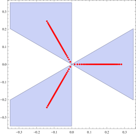
(a) Eigenvalues of the $Z_{3}$ solution for $N=123$, $\tilde{\lambda}=0.02$

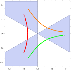
(b) Eigenvalues of the three single-cut solutions for $N=51$, $\tilde{\lambda}=0.1$

Figure 1: Eigenvalues for the pure CS model at weak coupling. The blue regions are the integration regions in the complex plane where $\mbox{Re}(\phi^{3})>0$ so that the path integral converges. The distributions were computed numerically using the heat equation on (8).

The $Z_{3}$ solution can also be obtained from (11) and (12) by setting the filling fraction parameter $B=0$. In this limit the side of one of the two cuts collides with a branch point of the other cut, leaving three symmetric cuts.

The single-cut solutions obtained from (15) by setting $\kappa=0$ are not $Z_{3}$-symmetric, but transform into each other under $Z_{3}$ transformations. For $U(N)$ the eigenvalue density has the form in (16) where $b$ satisfies

$$b^{3}=-\frac{\tilde{\lambda}}{\pi}\,.$$ (28)

This equation has three roots corresponding to the three different solutions, as shown in fig. 1(b). If one attempts to generate single-cut $SU(N)$ solutions using the eigenvalue density in (16) with

$$b^{3}=-\frac{\tilde{\lambda}}{4\pi}\,,$$ (29)

it does not work. Starting at one of the branch points and following a trajectory such that $\rho(\phi)d\phi$ is positive definite, one finds that the curve runs out to infinity instead of to the other branch point. From this we conclude that there are no single-cut solutions for $SU(N)$.

We next consider the free-energy for the $Z_{3}$ and the single-cut solutions. In the large-$N$ limit the free-energy is given by

$$F=\frac{kN\pi}{3}\int_{\mathcal{C}}\phi^{3}\rho(\phi)d\phi-\frac{N^{2}}{2}\int_{\mathcal{C}}d\phi d\phi^{\prime}\rho(\phi)\rho(\phi^{\prime})\log(\phi-\phi^{\prime})^{2}-N^{2}C$$ (30)

where the contour $\mathcal{C}$ is determined by the filling parameter $B$ in the resolvent. The last term in (30) comes from the first subleading term in the expansion of the full matrix model potential. Carrying out the expansion, one finds

$$C=\frac{1}{8}\log 2+\log\pi+\frac{7\zeta(3)}{16\pi^{2}}$$ (31)

Details for computing the integrals in (30) can be be found in Appendix B, where we show that

$$F = N^{2}\left(\frac{1}{2}-\frac{1}{3}\log\frac{\tilde{\lambda}}{\pi}-C\right)$$ (32)

for the $Z_{3}$ solution and

$$F = N^{2}\left(\frac{1}{2}-\frac{1}{3}\log\frac{\tilde{\lambda}}{\pi}+\frac{1}{2}\log 2-C\right)\,.$$ (33)

for the single-cut solutions. The free-energy for both solutions scales as $N^{2}$, but the $Z_{3}$ solution has lower free-energy and is thus the energetically preferable cut configuration.

The cut configuration is actually determined by the choice of an integration contour Witten:2010cx ; Felder:2004uy . In order for the path integral to converge the integration over the eigenvalues must asymptote into the blue regions in fig. 1. Each eigenvalue integral then connects two of the three regions. One of the regions has to be the one that covers the positive real axis if we are to have a solution that continuously connects onto the pure Yang-Mills solution. This would then exclude the single-cut solution shown in red dots in fig. 1(b). If the other end of the integration region is the same for all eigenvalues, then this would correspond to one of the two remaining single-cut solutions. However, if half the eigenvalues asymptote into the region bordering the positive imaginary axis and the other half into the region bordering the negative imaginary axis, then this gives the $Z_{3}$-symmetric configuration.

4 Strong coupling with adjoint matter

We now suppose that the couplings are large, $\lambda,\tilde{\lambda}\gg 1$. We can then assume that $|\mbox{Re}(\phi_{i}-\phi_{j})|\gg 1$ for most $i$ and $j$, in which case we can approximate (LABEL:eom) as

$$N\frac{\pi}{\tilde{\lambda}}(\phi^{2}_{i}+2\kappa\phi_{i}+\mu)=\left(\frac{9}{4}+m^{2}\right)\pi\sum\limits_{j\neq i}\mathrm{sign}(\mbox{Re}(\phi_{i}-\phi_{j}))\,.$$ (34)

Assuming that the $\mbox{Re}(\phi_{i})$ are ordered, we get the relation

$$\phi^{2}_{i}+2\kappa\phi_{i}+\mu=\chi\,\frac{2i-N}{N}\,,$$ (35)

and an eigenvalue density

$$\rho(\phi)=\frac{1}{\chi}(\phi+\kappa)\,,$$ (36)

where

$$\chi\equiv{\left(\frac{9}{4}+m^{2}\right)\tilde{\lambda}}\,.$$ (37)

In the $U(N)$ case with $\mu=0$, this means that the eigenvalues range between $\phi_{-}$ and $\phi_{+}$, where

$$\phi_{\pm}=-\kappa+\sqrt{\kappa^{2}\pm\chi}\,.$$ (38)

It is then clear that a transition occurs when the argument of the square root in $\phi_{-}$ vanishes, which occurs when

$$\kappa=\kappa_{crit}\equiv\chi^{1/2}=\frac{\sqrt{9+4m^{2}}}{2}\,\tilde{\lambda}^{1/2}\,.$$ (39)

Similar to weak coupling, all eigenvalues lie on the real line when $\kappa$ is above (39), but some are complex when $\kappa$ is below (39).

In the $SU(N)$ case we must set

$$\int_{\phi_{-}}^{\phi_{+}}\rho(\phi)\phi\,d\phi=0\,,$$ (40)

which leads to the relation

$$\mbox{$\frac{1}{3}$}\phi_{+}^{3}+\mbox{$\frac{1}{2}$}\kappa\phi^{2}_{+}=\mbox{$\frac{1}{3}$}\phi_{-}^{3}+\mbox{$\frac{1}{2}$}\kappa\phi^{2}_{-}\,,$$ (41)

where $\phi_{+}$ and $\phi_{-}$ are again the endpoints of the eigenvalue distribution. Combining this with the relations

$$\phi_{+}^{2}+2\kappa\phi_{+}-\mu = \chi$$

$$\phi_{-}^{2}+2\kappa\phi_{-}-\mu = -\chi\,,$$ (42)

we obtain the sytem of three equations that define the endpoints of the cut $\phi_{\pm}$ and the Lagrange multiplier $\mu$.

Introducing new variables $\psi_{\pm}\equiv\phi_{+}\pm\phi_{-}$, we can rewrite (41) and (4) as

$$\psi_{+}\psi_{-}+2\kappa\psi_{-} = 2\chi\,$$

$$\psi_{+}(\psi_{+}+\kappa)+2\mu = 0\,$$

$$\frac{4}{3}\,\chi^{2}+\psi_{+}(\psi_{+}+2\kappa)^{3} = 0\,.$$ (43)

This last equation has a critical point when

$$(\psi_{+}+2\kappa)^{3}+3\psi_{+}(\psi_{+}+2\kappa)^{2}=0\,,$$ (44)

which is satisfied when $\psi_{+}=-\kappa/2$. Substituting back into (43), we find

$$\kappa_{crit}=\frac{2\sqrt{2}}{3}\,\chi^{1/2}=\mbox{$\frac{1}{3}$}\sqrt{2(9+4m^{2})\tilde{\lambda}}$$ (45)

for the critical value. In section (7) we will further study these critical points, where we will show that the phase transition stays third-order for strong coupling.

4.1 Chern-Simons with adjoint matter

We now assume that $\kappa=0$ such that the theory is pure CS and we are past the phase transition. As we move to stronger coupling for $\tilde{\lambda}$, the $Z_{3}$ symmetry breaks as the determinant factors diverge from the Vandermonde form. We still expect there to be the analog of the three single-cut solutions in section 3.1, that is one solution with an eigenvalue distribution symmetric about the real axis and the other two complex conjugates of each other. We also expect an analog of the $Z_{3}$ solution, which has a branch on the real line and two complex branches that are conjugate to each other. We still assume that $|\mbox{Re}(\phi_{i}-\phi_{j})|\gg 1$ for generic eigenvalues and that the $\mbox{Re}(\phi_{i})$ are ordered. Hence, the eigenvalues still satisfy (35) and (36), with $\kappa=0$.

For the case of $U(N)$ with $\mu=0$, we see that the the righthand side of (35) is positive if $i\geq N/2$, hence these eigenvalues are on the positive real line and run between the origin and $\phi_{+}=\sqrt{\tilde{\lambda}({9}/{4}+m^{2})}$. However, for $i<N/2$, the righthand side of (35) is negative and the corresponding eigenvalues lie on the imaginary axis. If the imaginary eigenvalues have the same sign, then the solution connects to one of the complex single-cut solutions at weak coupling and the free-energy is complex. Alternatively, the eigenvalues could divide up such that the imaginary eigenvalues appear with their conjugates, in which case the free-energy is real. We will continue to refer to this as the $Z_{3}$ solution since this is the one that connects to the $Z_{3}$ weak coupling solution.

Note that these branches cannot lie exactly on the imaginary axes, since the approximations used for $\coth\pi(\phi_{i}-\phi_{j})$ and $\tanh\pi(\phi_{i}-\phi_{j})$ break down if the real part of the argument is zero. Instead we should assume that the eigenvalues satisfy $|\mbox{Im}(\phi_{i}-\phi_{j})|\gg|\mbox{Re}(\phi_{i}-\phi_{j})|\gg 1$, with the ratio of the imaginary to the real parts diverging as $\tilde{\lambda}\to\infty$. A numerical solution of (LABEL:eom) at strong coupling is shown in fig. 2 and confirms these assumptions. As shown in the figure, half of the eigenvalues lie on the positive real axis, while the other half spread in the general direction of the positive imaginary axis, but with some separation along the real axis. Furthermore, the endpoint toward the imaginary direction is close to the computed value $\phi_{-}$.

We also see from the numerical solution that the distribution of the eigenvalues along the imaginary axis is somewhat chaotic. This is partly due to the poles of the coth and tanh functions along the imaginary axis which lead to less numerical precision.

But more importantly, for high enough $\tilde{\lambda}$, the single-cut solution no longer exists and the cut starts bifurcating into multi-cuts along the imaginary direction, with the number of cuts scaling as $\tilde{\lambda}^{1/2}$. We interpret the bifurcating of the cuts as evidence for phase transitions as $\tilde{\lambda}^{1/2}$ is increased. In appendix C we show the disappearance of the single-cut solution explicitly by considering the solution for the special point $m^{2}=-1/4$, where the matrix model is solvable analytically. Here we find a critical value $\tilde{\lambda}_{c}\approx 0.976$ where the eigenvalue density goes to zero in the middle of the cut, signifying a splitting into two cuts. We also argue that a new cut appears when $\sqrt{2}\,\tilde{\lambda}^{1/2}$ is increased by $2$. More generally, we believe that a new cut appears when $\chi^{1/2}$ increases by $2$. Each appearance of a new cut signifies a phase transition. The existence of the phase transitions complicates the search for supergravity duals, and perhaps indicates that they do not exist.

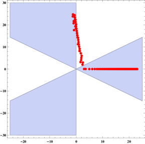
Figure 2: Example of strong coupling solution $\tilde{\lambda}=750$, $N=87$.

Turning to $SU(N)$, it is straightforward to show that continuous solutions to (35) with $\kappa=0$ do not exist. Setting $\kappa=0$ in (41) and (4), we are immediately led to

$$\chi^{3}+3\mu^{2}\,\chi=0\,,$$ (46)

and so

$$\mu=\pm\frac{i}{\sqrt{3}}\,\chi\,.$$ (47)

Hence, the endpoints of the eigenvalue distribution consistent with (41) are at

$$\phi_{+}=\frac{\sqrt{2}}{3^{1/4}}\,\chi^{1/2}\,e^{\pm i\pi/12}\,,\quad\phi_{-}=-\frac{\sqrt{2}}{3^{1/4}}\,\chi^{1/2}\,e^{\pm 7i\pi/12}\,.$$ (48)

But these endpoints cannot be connected by a continuous distribution of eigenvalues because they lie on different branches. However, we believe there is an approximate solution where $\mu=\chi$, making $\phi_{i}$ imaginary for all $i$. Assuming that the conjugates also appear, then $\langle\phi\rangle=0$, satisfying the traceless condition.

Figure 3: $\tilde{\lambda}$-dependence of the free energy at strong coupling. The orange dots represent the numerical solution while the dashed blue line is the solution in (52).

Returning to the $U(N)$ case and using our assumptions about the eigenvalues, we can approximate the free energy as

$$F\equiv-\log Z \approx \sum_{i}\frac{\pi k}{3}\phi_{i}^{3}-\frac{(9+4m^{2})\pi}{4}\sum_{i<j}|\mbox{Re}(\phi_{i}-\phi_{j})|\,.$$ (49)

For the $Z_{3}$ solution this becomes

$$F\approx \sum_{i>N/2}\frac{\pi k}{3}\phi_{i}^{3}-\frac{(9+4m^{2})\pi}{4}\frac{N}{2}\sum_{i>N/2}\phi_{i}-\frac{(9+4m^{2})\pi}{4}\sum_{N/2<i<j}(\phi_{j}-\phi_{i})\,,$$ (50)

where the leading contributions from the two complex branches have canceled out. Then plugging (35) into (50), we find

$$F\approx-\frac{(9+4m^{2})^{3/2}\pi}{60}N^{2}\tilde{\lambda}^{1/2}\,,$$ (51)

which simplifies to

$$F\approx-\frac{9\pi}{20}N^{2}\tilde{\lambda}^{1/2}$$ (52)

at the superconformal point. For the solutions that have all of their complex roots either above or below the real line, the free-energy is complex, but the real part matches (51).

Substituting $\tilde{\lambda}=N/k$ into (51) and (52), we find $N^{5/2}$ behavior for the free-energy at strong coupling. This parallels the strong-coupling behavior of the $5D$ superconformal theories in Jafferis:2012iv . In our case, by adjusting $\kappa$ we can transition between the $N^{3}$ behavior that one finds for SYM, which is related to the behavior of $6D$ superconformal theories, and $N^{5/2}$ behavior which is expected for $5D$ superconformal theories. Note that the $SU(N)$ theories will not have the $N^{5/2}$ behavior, because in the leading approximation their eigenvalues lie on the imaginary axis and so their contribution to the free-energy cancels.

As a further check on our results, we computed the real part of the free-energy numerically as a function of $\tilde{\lambda}$ for the solution in fig. 2. The results of this analysis are shown in fig. 3. Here we see that the approximate result in (52) accurately reproduces the numerical result.

5 Wilson Loops

A supersymmetric Wilson loop wrapping the equator of $S^{5}$ can also be obtained from the matrix model in (3). Such loops were considered in Young:2011aa and Minahan:2013jwa for $5D$ $SU(N)$ SYM theory and in Assel:2012nf for $5D$ superconformal theories. One twist to the situation here is that the CS term in the action is odd under charge conjugation, hence the Wilson loop for the fundamental representation can be different from the Wilson loop in the anti-fundamental representation.

The expectation value of the Wilson loop in the fundamental or anti-fundamental representation, after localizing, is the expectation value in the matrix model (3) Pestun:2007rz ,

$$\langle W\rangle^{\pm}=\frac{1}{N}\langle\textrm{Tr}\,e^{\pm 2\pi\phi}\rangle\,,$$ (53)

where the $+$ ($-$) sign refers to the (anti-) fundamental representation. In the large-$N$ limit the back-reaction of this term on the eigenvalue distribution is negligible, hence the expectation value of the loop is well approximated by

$$\langle W\rangle^{\pm}=\int d\phi\rho(\phi)e^{\pm 2\pi\phi}\,,$$ (54)

where $\rho(\phi)$ is the eigenvalue density computed in the previous sections.

In the rest of this section we consider the Wilson loop for the pure CS models at weak and strong coupling.

5.1 Purely cubic model at weak coupling

At weak coupling we have studied two types of solutions, the $Z_{3}$ solution and the single-cut solutions. Let us consider Wilson loops for these configurations separately.

5.1.1 $Z_{3}$ symmetric solution

The $Z_{3}$ solution is given by (12) with $B=\kappa=\mu=0$. This solution consists of three branches that can be mapped into each other by $e^{2\pi i/3}$ rotations. All three branches contribute to the integral (54), leading to the expression

$$\langle W\rangle_{Z_{3}}^{\pm}=\int\limits_{0}^{\phi^{*}}d\phi\frac{\phi^{2}}{2\tilde{\lambda}}\sqrt{\frac{4\tilde{\lambda}}{\pi\phi^{3}}-1}\left[e^{\pm 2\pi\phi}+e^{\pm\pi\phi(-1+\sqrt{3}i)}+e^{\pm\pi\phi(-1-\sqrt{3}i)}\right]\,,$$ (55)

where the first term in the square brackets comes from the integration over the branch on the real line, while the two other terms come from the rotated branches. The endpoint of the cut on the real line sits at $\phi^{*}=({4\tilde{\lambda}}/{\pi})^{1/3}$.

The integral results in the generalized hypergeometric function

$$\langle W\rangle_{Z_{3}}^{\pm}=~{}_{1}F_{3}\left(\frac{1}{2};\frac{1}{3},\frac{2}{3},2;\pm\frac{32\pi^{2}\tilde{\lambda}}{27}\right)\,.$$ (56)

This expression is real and in the limit $\tilde{\lambda}\ll 1$ its log is approximately

$$\log\langle W\rangle^{\pm}_{Z_{3}}\approx\pm\frac{4\pi^{2}\tilde{\lambda}}{3}$$ (57)

5.1.2 Single-cut solutions

The three single-cut solutions for $U(N)$ have $\kappa=\mu=0$ in (16), with $b$ one of the roots in (28). The real root corresponds to the solution symmetric with respect to the real axis, while the other roots correspond to the single cuts that are completely above or below the real axis.

For the symmetric solution the Wilson loop is given by the integral

$$\langle W\rangle_{Z_{2}}^{\pm}=\int\limits_{\phi_{1}}^{\phi_{2}}d\phi\frac{i}{2\tilde{\lambda}}\left(\phi-\left(\frac{\tilde{\lambda}}{\pi}\right)^{1/3}\right)\sqrt{(\phi-\phi_{1})(\phi-\phi_{2})}~{}e^{\pm 2\pi\phi},$$ (58)

where

$$\phi_{1}=({\tilde{\lambda}}/{\pi})^{1/3}(-1-i\sqrt{2})\,,\qquad\phi_{2}=({\tilde{\lambda}}/{\pi})^{1/3}(-1+i\sqrt{2})\,.$$ (59)

Defining the new variable $x=\frac{1}{i\sqrt{2}}\left(({\tilde{\lambda}}/{\pi})^{1/3}\phi+1\right)$, we can rewrite (58) as

$$\langle W\rangle_{Z_{2}}^{\pm}=-2\int\limits_{-1}^{1}(\sqrt{2}ix-2)\sqrt{1-x^{2}}e^{a(i\sqrt{2}x-1)}$$ (60)

where $a=\pm(8\pi^{2}\tilde{\lambda})^{1/3}$. The integral then gives

$$\langle W\rangle_{Z_{2}}^{\pm}=\frac{e^{-a}}{a}\left(a~{}_{0}F_{1}\left(2,-\frac{a^{2}}{2}\right)+J_{2}\left(\sqrt{2}a\right)\right)$$ (61)

where ${}_{0}F_{1}$ is the confluent hypergeometric function. This expression is real and for $\tilde{\lambda}\ll 1$ its log behaves as

$$\log\langle W\rangle_{Z_{2}}^{\pm}\approx\mp\frac{3}{2}(\pi^{2}\tilde{\lambda})^{1/3}\,.$$ (62)

The Wilson loop for the other two single-cut solutions can be found by rotating $\phi$ in (58) by $e^{\pm 2\pi i/3}$. This is equivalent to rotating $a$ in (61) by $e^{\pm 2\pi i/3}$. Hence for $\lambda\ll 1$ the log of the Wilson loops for these configurations are

$$\log\langle W\rangle_{n}^{\pm}\approx\mp\frac{3}{2}(\pi^{2}\tilde{\lambda})^{1/3}e^{2\pi in/3}\,.$$ (63)

Note that there is significantly different behavior between the Wilson loops for the $Z_{3}$ solution and the single-cut solutions. Not only is the power of $\tilde{\lambda}$ different between (57) and (62), but so too is the sign.

5.2 Pure CS model at strong coupling

We next consider the Wilson loops in the strong coupling limit where $\tilde{\lambda}\gg 1$. We first consider configurations where the imaginary eigenvalues are all above the real axis, as in fig. 2. Substituting the density in (36) into the integral (54) with $\kappa=0$, we obtain

$$\langle W\rangle_{strong}^{\pm}=\int\limits_{C}d\phi~{}\frac{\phi~{}e^{\pm 2\pi\phi}}{\chi},$$ (64)

where $\chi$ is defined in (37) and the contour $C$ runs along the real axis up to $\phi_{+}=\chi^{1/2}$ and the imaginary axis to $\phi_{-}=i\chi^{1/2}$. Evaluating the integral, we obtain a complex result with components

$$\mbox{Re}\left(\langle W\rangle_{strong}^{\pm}\right) = \frac{1}{2\pi\chi}\left(\left(\pm\chi^{\mbox{$\frac{1}{2}$}}-\frac{1}{2\pi}\right)e^{\pm 2\pi\chi^{1/2}}+\chi^{\mbox{$\frac{1}{2}$}}\sin{2\pi\chi^{\mbox{$\frac{1}{2}$}}}+\frac{1}{2\pi}\cos{2\pi\chi^{\mbox{$\frac{1}{2}$}}}\right)\,,$$ (65)

$$\mbox{Im}\left(\langle W\rangle_{strong}^{\pm}\right) = \pm\frac{1}{2\pi\chi}\left(\frac{1}{2\pi}\sin{2\pi\chi^{1/2}}-\chi^{1/2}\cos{2\pi\chi^{1/2}}\right)\,.$$ (66)

Since $\tilde{\lambda}\gg 1$, there is clearly a significant difference between $\langle W\rangle^{+}$ and $\langle W\rangle^{-}$. In the former case, the real component is approximately

$$\mbox{Re}\left(\langle W\rangle^{+}_{strong}\right)\approx\frac{1}{2\pi}\,\chi^{-1/2}\,e^{2\pi\chi^{1/2}}\,,$$ (67)

while $\mbox{Im}\left(\langle W\rangle^{+}_{strong}\right)\rightarrow 0$ at strong coupling when $\tilde{\lambda}\gg 1$. Therefore, the log of the Wilson loop is approximately

$$\log\left(\langle W\rangle^{+}_{strong}\right)\approx 2\pi\,\chi^{1/2}=2\pi\sqrt{\tilde{\lambda}\left(\frac{9}{4}+m^{2}\right)}$$ (68)

In the case of $\langle W\rangle^{-}$, the real part does not have the exponentially growing piece in (67), therefore its log is much smaller than (68).

For the $Z_{3}$ configuration, where each complex eigenvalue appears with its conjugate, $\mbox{Im}\left(\langle W\rangle^{\pm}\right)$ cancels, while $\mbox{Re}\left(\langle W\rangle^{+}\right)$ is still dominated by the real end-point, thus the log is also given by (68).

6 Chern-Simons quivers

All results in the previous sections can be generalized to different types of quiver theories. Some examples of $5D$ quivers where considered in Bergman:2012kr , Bergman:2013aca , Kallen:2012zn and Minahan:2013jwa . But these all considered quivers with pure Yang-Mills terms in the nodes. Here we will consider quivers with $\mathcal{N}=1$ $U(N)$ Chern-Simons vector multiplets in the nodes and with hypermultiplets in bifundamental representations. These quivers are more similar to the ones considered in Imamura:2008nn , Herzog:2010hf or in the simplest case of two nodes in ABJM theory Aharony:2008ug

The first type of quivers we consider are necklace quivers with $n$ nodes. Each of the nodes contain $U(N)$ $\mathcal{N}=1$ Chern-Simons with equal levels $k$ and matter multiplets in the bifundamental representation. This type of quiver is shown schematically in fig. 4(a). The eigenvalues in the saddle-point equations (LABEL:eom) split into $n$ groups $\psi_{i}^{(r)}$ with $r=1,\dots,n$ and $i=1,\dots,N$ and the equations in the planar limit take the form

$$\frac{\pi N}{\tilde{\lambda}}(\psi^{(r)}_{i})^{2} = \pi\Big{[}\sum\limits_{j\neq i}\left(2-(\psi^{(r)}_{i}-\psi^{(r)}_{j})^{2}\right)\coth(\pi(\psi^{(r)}_{i}-\psi^{(r)}_{j}))$$ (69)

$$\qquad+\Bigg{(}\sum_{j}\Big{[}\mbox{$\frac{1}{4}$}\left(\mbox{$\frac{1}{4}$}+(\psi^{(r)}_{i}\!-\!\psi^{(r\!+\!1)}_{j}\!-\!m)^{2}\right)\tanh(\pi(\psi^{(r)}_{i}\!-\!\psi^{(r\!+\!1)}_{j}\!-\!m))$$

$$\qquad\qquad+\mbox{$\frac{1}{4}$}\left(\mbox{$\frac{1}{4}$}+(\psi^{(r)}_{i}\!-\!\psi^{(r\!-\!1)}_{j}\!-\!m)^{2}\right)\tanh(\pi(\psi^{(r)}_{i}\!-\!\psi^{(r\!-\!1)}_{j}\!-\!m))\Big{]}\Big{]}$$

$$\qquad\qquad\qquad+(m\to-m)\Bigg{)}\,.$$

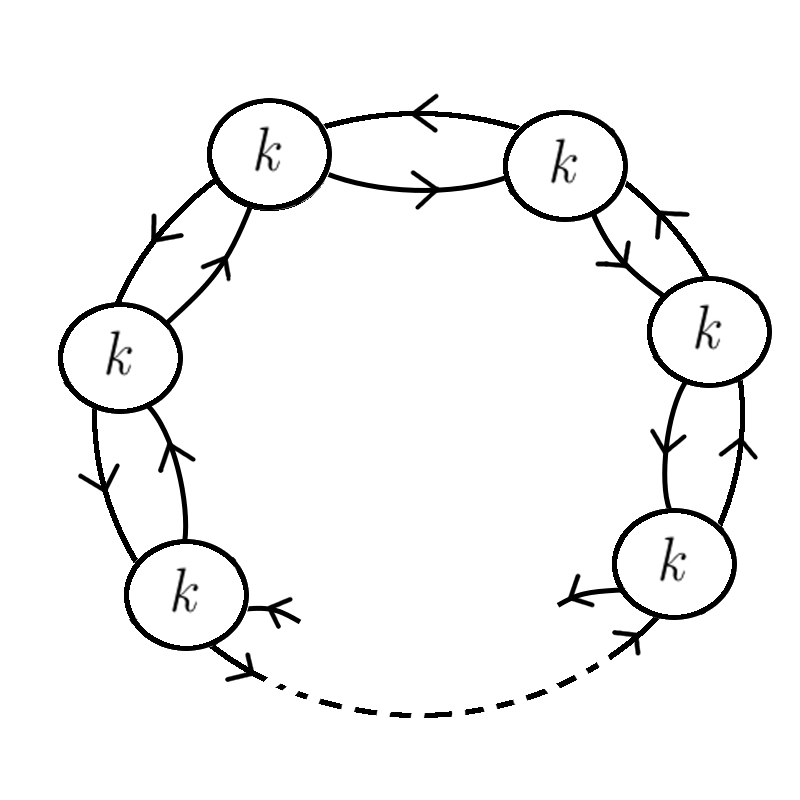
(a) Necklace quiver CS theory with equal levels in all nodes

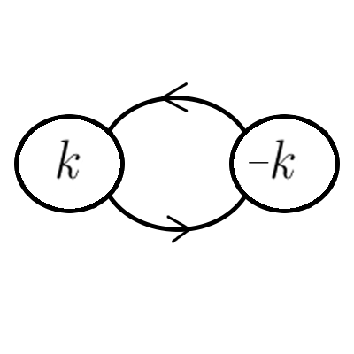
(b) ABJM-like quiver theory

Figure 4: Schematical representations of different Chern-Simons quiver theories

These equations have the obvious solution $\psi_{i}^{(r)}=\psi_{i}^{(s)}$ for all $r$ and $s$. The eigenvalues of each quiver satisfy the same saddle-point equations as a single-node theory (LABEL:eom). Thus, the solution at strong coupling is given by

$$\phi^{(r)}_{i}=\sqrt{\frac{\left(9+4m^{2}\right)\tilde{\lambda}}{4}\frac{2i-N}{N}}\,,$$ (70)

In the case where $m=0$, we get the same free-energy as in (52), multiplied by the number of nodes $n$,

$$F\approx-\frac{9\pi}{20}N^{2}\tilde{\lambda}^{1/2}n\,.$$ (71)

Likewise, for the Wilson loops we get the same asymptotic behavior as for the single-node theory,

$$\log\left(\langle W\rangle_{quiv.}\right)\approx 2\pi\sqrt{\tilde{\lambda}\left(\frac{9}{4}+m^{2}\right)}$$ (72)

The solution we have described above is the only one we aware of for the quiver theories. Furthermore, numerical simulations do not show the presence of any other solutions, although a more accurate study of the equations (69) could reveal other solutions.

Another type of quiver theory that can be easily generalized from the single-node solution is an ABJM-like theory with two nodes. Like ABJM, each node has a $U(N)$ Chern-Simons but with opposite levels $k$ and $-k$. There are also bifundamental matter fields connecting the two nodes (see fig. 4(b)).

Denoting the eigenvalues of each node by $\phi_{i}$ and $\psi_{i}$, we can write down the equations of motion

$$\frac{\pi N}{\tilde{\lambda}}\phi^{2}_{i}=\pi\sum\limits_{j\neq i}\left(2-(\phi_{i}-\phi_{j})^{2}\right)\coth(\pi(\phi_{i}-\phi_{j}))$$

$$\qquad+\pi\sum\limits_{j}\Bigg{[}\frac{1}{2}\left(\frac{1}{4}+(\phi_{i}-\psi_{j}-m)^{2}\right)\tanh(\pi(\phi_{i}-\psi_{j}-m))+(m\to-m)\Bigg{]}\,,$$ (73)

$$-\frac{\pi N}{\tilde{\lambda}}\psi^{2}_{i}=\pi\sum\limits_{j\neq i}\left(2-(\psi_{i}-\psi_{j})^{2}\right)\coth(\pi(\psi_{i}-\psi_{j}))$$

$$\qquad+\pi\sum\limits_{j}\Bigg{[}\frac{1}{2}\left(\frac{1}{4}+(\psi_{i}-\phi_{j}-m)^{2}\right)\tanh(\pi(\psi_{i}-\phi_{j}-m))+(m\to-m)\Bigg{]}\,.$$ (74)

Because of the symmetry properties of the cubic Chern-Simons term, these equations have the very nice solution $\phi_{i}=-\psi_{i}$. Hence, the effective equation for the single node takes the form

$$\frac{\pi N}{\tilde{\lambda}}\phi^{2}_{i}=\pi\sum\limits_{j\neq i}\left(2-(\phi_{i}-\phi_{j})^{2}\right)\coth(\pi(\phi_{i}-\phi_{j}))$$

$$\qquad+\pi\sum\limits_{j}\Bigg{[}\frac{1}{2}\left(\frac{1}{4}+(\phi_{i}+\phi_{j}-m)^{2}\right)\tanh(\pi(\phi_{i}+\phi_{j}-m))+(m\to-m)\Bigg{]}\,.$$

(75)

Notice that here we cannot assume that $|\mbox{Re}(\phi_{i}-\phi_{j})|\gg 1$ for generic eigenvalues since the quadratic terms $(\phi_{i}-\phi_{j})^{2}$ and $(\phi_{i}+\phi_{j})^{2}$ on the r.h.s do not cancel each other. This makes it difficult to find approximate equations of motion with analytic solutions.

Though we can’t say much about the behavior of the solutions of (75) from analytical calculations, we were able to find different numerical solutions of this quiver model. The results of the numerical simulations are shown in fig. 5. For these solutions we can clearly see that the eigenvalues do not satisfy $|\mbox{Re}(\phi_{i}-\phi_{j})|\gg 1$.

For the solution in fig. 5(a) the eigenvalues are distributed symmetrically about the real axis and lie close to, but not exactly on the imaginary axis. Furthermore, the separation between the endpoints stays finite even for large $\tilde{\lambda}$, a behavior that is also seen for the solution in (156) for pure Chern-Simons with $m^{2}=-1/4$. For the solution shown in fig. 5(b) the eigenvalues also lie close to imaginary axis. However they are clearly not symmetric with respect to real axis as they all lie in the lower half-plane. In this case the distance between the endpoints increases with increasing $\tilde{\lambda}$.

Since all the eigenvalues for these solutions lie close to the imaginary axis, the real part of the free energy cannot go beyond the usual $N^{2}$ dependence.

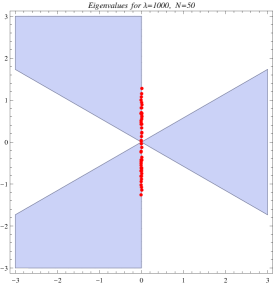
(a) First kind of solutions to (75) $N=50$, $\tilde{\lambda}=1000$, $m=0$

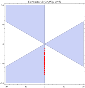
(b) First kind of solutions to (75) $N=51$, $\tilde{\lambda}=1000$, $m=0$

Figure 5: Eigenvalues for the ABJM-like quiver model at strong coupling. The blue regions are the integration regions in the complex plane where $\mbox{Re}(\phi^{3})>0$ so that the path integral converges.

7 The SYM-CS phase transition

In this section we elaborate on the phase transition between super Yang-Mills and Chern-Simons behavior. The main result is that the phase transition is third order for both weak and strong coupling.

7.1 $U(N)$

We start with the $U(N)$ theory at weak coupling. Part of this analysis has previously appeared in the context of triangulated surfaces in 2D gravity David:1984tx ; Ambjorn:1985az ; Kazakov:1985ea ; Boulatov:1986jd , but we include it for completeness. We wish to explore the behavior of the free-energy near the critical point, $\kappa^{2}=3\,b^{2}$, where $\kappa$ and $b$ satisfy (14) with $\mu=0$. We first write $\kappa$ and $B$ in terms of two small parameters $\epsilon$ and $\delta$,

$$\kappa^{2}={3}\,L^{2/3}-\epsilon\,,\qquad B=-12L^{4/3}+4L^{2/3}\epsilon+L^{1/3}\delta\,,$$ (76)

where $L\equiv(\tilde{\lambda}/2\pi)=\kappa_{crit}^{3}/(3\sqrt{3})\,$. The free-energy in the large $N$ limit is given by

$$F=N^{2}\left(\frac{1}{2L}\int_{\mathcal{C}}d\phi\rho(\phi)(\mbox{$\frac{1}{3}$}\phi^{3}+\kappa\phi^{2}-\mbox{$\frac{2}{3}$}\kappa^{3})-\frac{1}{2}\int_{\mathcal{C}}d\phi d\phi^{\prime}\rho(\phi)\rho(\phi^{\prime})\log(\phi-\phi^{\prime})^{2}\right)\,,$$ (77)

where we subtracted off a constant piece to simplify expressions, but will otherwise not effect the phase structure. Using the more general expression for $\rho(\phi)$ in (12), the free-energy, as an expansion in $\epsilon$ and $\delta$, is found to be

$$F=N^{2}\left(-\frac{3}{4}-\frac{1}{3}\log L+\frac{3}{4}\,L^{-2/3}\epsilon-\frac{1}{8}\,L^{-4/3}\epsilon^{2}-\frac{1}{40}\,L^{-5/3}\epsilon\,\delta+\dots\right)\,,$$ (78)

where the expression is valid on either side of the phase transition.

Below the transition we have $\epsilon<0$ with a single-cut eigenvalue distribution. Hence, $B$ has the form in (13). If we write $b=L^{1/3}+\beta$, then (13) implies

$$B=-12L^{4/3}+8L^{2/3}\epsilon+12L^{2/3}\beta^{2}+4L^{1/3}\epsilon\,\beta+12L^{1/3}\beta^{3}+\dots\,,$$ (79)

while (14) reduces to

$$L^{1/3}\epsilon+3L^{1/3}\beta^{2}+\epsilon\,\beta+\beta^{3}=0\,.$$ (80)

Solving this last equation for $\beta$ in terms of $\epsilon$ and substituting into (79), we find

$$B=-12L^{4/3}+4L^{2/3}\epsilon+8L^{1/3}(-\epsilon/3)^{3/2}+\dots\,.$$ (81)

Comparing this equation with (76), we find that $\delta\approx 8(-\epsilon/3)^{3/2}$, and so the free-energy becomes

$$F=N^{2}\left(\mbox{regular terms}+\frac{1}{15\sqrt{3}}L^{-5/3}\left(-{\epsilon}\right)^{5/2}+\dots\right)\,.$$ (82)

Hence, because the third derivative of $F$ diverges at this point, there is a third-order phase transition at $\epsilon=0$.

Let us now continue above the transition to $\epsilon>0$. We assume that the eigenvalues lie on the symmetric two-cut solution that connects to the $Z_{3}$ solution as $\kappa\to 0$. At the critical point, three of the four branch points in (12) meet at ${\tilde{\phi}}=-L^{1/3}$. As we move away from the critical point by increasing $\epsilon$, the branch points spread apart, and the density near these points is approximately

$$\rho(\delta\phi)\approx\frac{1}{4\pi L^{5/6}}\sqrt{4\delta\phi^{3}+4\epsilon\delta\phi-\delta}\,,$$ (83)

where $\delta\phi={\tilde{\phi}}+L^{1/3}$. We can shift one of the branch points to zero by setting $\delta\phi=\Delta\phi+x$, where $\Delta\phi$ satisfies the equation

$$4\Delta\phi^{3}+4\epsilon\Delta\phi-\delta=0\,.$$ (84)

In terms of $x$, the density is

$$\rho(x)=\frac{1}{2\pi L^{5/6}}\sqrt{x(x^{2}+3\Delta\phi x+3\Delta\phi^{2}+\epsilon)}\,.$$ (85)

Assuming that $\epsilon>0$, we see that two of the branch points are at

$$x=-\frac{3\Delta\phi}{2}\pm\frac{i\Delta\phi}{2}\sqrt{3+\frac{4\epsilon}{\Delta\phi^{2}}}\equiv re^{\pm i\theta}\,.$$ (86)

In the limit that $\epsilon\to 0$, $\Delta\phi$ , $\delta$ and $r$ all approach zero.

To determine the correct value of $\theta$, we now insist that the integral of $\rho(x)$ from $x=0$ to $x=re^{i\theta}$ is positive definite. We can do the integral, which gives

$$\int_{0}^{re^{i\theta}}\rho(x)dx=\frac{1}{2\pi L^{5/6}}\int_{0}^{re^{i\theta}}dx\sqrt{x(x^{2}-2r{x}\cos\theta+r^{2})}$$

$$= \frac{r^{5/2}}{15\pi L^{5/6}}\sqrt{-2i\sin\theta}\left(2(2\cos{2}\,\theta-1)E\left(\frac{1}{1-e^{2i\theta}}\right)+\left(1-2e^{-2i\theta}\right)K\left(\frac{1}{1-e^{2i\theta}}\right)\right)\,,$$

where $K$ and $E$ are the complete elliptic integrals of the first and second kind. We then adjust $\theta$ such that (7.1) is positive real. This can be done numerically, where we find

$$\theta\approx(0.637775)\,\pi\,.$$ (88)

Hence the endpoints lie in the second and third quadrants.

It then follows from (86) that

$$\Delta\phi^{2}=\frac{{4}\,\epsilon}{9\tan^{2}\theta-3}\,,$$ (89)

which then can be used in (84) to give

$$\delta=\frac{8\epsilon^{3/2}}{(9\tan^{2}\theta-3)^{3/2}}(9\tan^{2}\theta+1)\approx(1.40907)\,\epsilon^{3/2}\,.$$ (90)

Substituting this into (78), the free-energy above the transition is given by

$$F=N^{2}\left(\mbox{regular terms}-(0.035223)\,L^{-5/3}\,\epsilon^{5/2}+\dots\right)\,.$$ (91)

Curiously, the coefficient of the $\epsilon^{5/2}$ term in (91) is within 10% of the coefficient of the $(-\epsilon)^{5/2}$ term in (82).

Because of the sign in front of the singular term, the free-energy in (91) is lower than the real part of the free-energy of the one-cut solution. This latter case is found by analytically continuing $\epsilon$ in (82) to the positive real axis. Hence the singular term is imaginary. The regular terms are the same in (82) and (91), showing that the two-cut solution is energetically favorable.

Turning now to the phase transition at strong coupling, we have that the density and endpoints of the integration are given by (36) and (38) respectively. If we are in the YM phase with $\kappa>\kappa_{crit}$, where $\kappa_{crit}$ is defined in (39), then the free-energy is well approximated by

$$F\approx N^{2}\left(\frac{\pi}{\tilde{\lambda}}\int_{\phi_{-}}^{\phi_{+}}d\phi\left(\mbox{$\frac{1}{3}$}\phi^{3}+\kappa\phi^{2}-\mbox{$\frac{2}{3}$}\kappa^{3}\right)\rho(\phi)-\frac{(9+4m^{2})\pi}{8}\int_{\phi_{-}}^{\phi_{+}}d\phi d\phi^{\prime}|\phi-\phi^{\prime}|\rho(\phi)\rho(\phi^{\prime})\right)\,.$$

Using the density and endpoints in (36) and (38), we find

$$F \approx N^{2}\frac{8\pi}{15(9+4m^{2})\,\tilde{\lambda}^{2}}\left(\left(\kappa^{2}-\frac{(9+4m^{2})\tilde{\lambda}}{4}\right)^{5/2}-\left(\kappa^{2}+\frac{(9+4m^{2})\tilde{\lambda}}{4}\right)^{5/2}\right)$$ (93)

$$= N^{2}\left(\mbox{regular terms}+\frac{8\pi}{15(9+4m^{2})\,\tilde{\lambda}^{2}}\,(-\epsilon)^{5/2}\right)\,,$$

where

$$\epsilon=\kappa^{2}_{crit}-\kappa^{2}\,,$$ (94)

and where $\kappa^{2}_{crit}=(9+4m^{2})\tilde{\lambda}/4$. Hence, the third-order phase transition persists at strong coupling.

On the CS side of the transition, the $\phi_{-}$ integration boundary in (7.1) should be replaced by $0$. In this case the free-energy is only made up of regular terms.

7.2 $SU(N)$

The $SU(N)$ theory has a Lagrange multiplier that could potentially change the nature of the phase transition. Here we show that although the details differ from the $U(N)$ case, the phase transition stays third order.

For weak coupling, we can carry out a similar analysis as for (82) in the $U(N)$ case, but also including the Lagrange multiplier $\mu$. We will only consider the system in the YM phase, in which case we can invoke the single-cut density in (16). Substituting this into (77), we can write $F$ as

$$F=N^{2}\left(-\frac{1}{2}\log\frac{L}{b}+\frac{L}{12b^{3}}+\frac{L^{2}}{96b^{6}}-\frac{\kappa^{3}}{3L}+\frac{12b^{2}\kappa-3b\kappa^{2}}{24b^{3}}+\frac{3}{8}\right)$$ (95)

where $b$ satisfies (19). The critical value for $\kappa$ is given in (22), which in terms of $L$ is $\kappa_{crit}=\mbox{$\frac{3}{2}$}L^{1/3}$. Using a slightly different parameterization than we did for the $U(N)$ case, we set $\kappa=\kappa_{crit}-\epsilon^{\prime}$. After substituting this into (19), we can write the series expansion for $b$ near the critical point as

$$b = L^{1/3}+\sqrt{\frac{2}{3}}L^{1/6}(-\epsilon^{\prime})^{1/2}+\frac{4}{9}(-\epsilon^{\prime})+\frac{5\sqrt{2}}{27\sqrt{3}}L^{-1/6}(-\epsilon^{\prime})^{3/2}$$ (96)

$$\qquad\qquad\qquad\qquad+\frac{4}{243}L^{-1/3}(-\epsilon^{\prime})^{2}-\frac{7}{243\sqrt{6}}L^{-1/2}(-\epsilon^{\prime})^{5/2}+\dots\,.$$

Putting this expression for $b$ into (95) we find

$$F=N^{2}\left(\mbox{regular terms}+\frac{4\sqrt{2}}{15\sqrt{3}}L^{-5/6}(-\epsilon^{\prime})^{5/2}\right)\,,$$ (97)

hence, the phase-transition is third order in the weak-coupling limit.

We can analyze the behavior at strong coupling by including the Lagrange multiplier $\mu$ in the eigenvalue density that appears in (7.1). This modifies the the first line of (93) to to

$$F \approx N^{2}\frac{4\pi}{3(9+4m^{2})\,\tilde{\lambda}^{2}}\Biggl{(}\frac{2}{5}\Biggl{[}\biggl{(}\kappa^{2}+\mu-\frac{(9+4m^{2})\tilde{\lambda}}{4}\biggr{)}^{5/2}-\biggl{(}\kappa^{2}+\mu+\frac{(9+4m^{2})\tilde{\lambda}}{4}\biggr{)}^{5/2}\Biggr{]}$$ (98)

$$\qquad\qquad-\mu\Biggl{[}\biggl{(}\kappa^{2}+\mu-\frac{(9+4m^{2})\tilde{\lambda}}{4}\biggr{)}^{3/2}-\biggl{(}\kappa^{2}+\mu+\frac{(9+4m^{2})\tilde{\lambda}}{4}\biggr{)}^{3/2}\Biggr{]}\Biggr{)}$$

Again writing $\kappa=\kappa_{crit}-\epsilon^{\prime}$, where $\kappa_{crit}$ is given in (45), and using (4) and (43) we can expand $\mu$ near the critical point,

$$\mu=\frac{1}{8}\kappa_{crit}^{2}-\frac{1}{2}\kappa_{crit}(-\epsilon^{\prime})+\frac{\sqrt{2}}{\sqrt{3}}\kappa_{crit}^{1/2}(-\epsilon^{\prime})^{3/2}-\frac{7}{12}(-\epsilon^{\prime})^{2}+\frac{7}{18\sqrt{6}}\kappa_{crit}^{-1/2}(-\epsilon^{\prime})^{5/2}+\dots$$

Inserting this into (98) and expanding, we find

$$F\approx N^{2}\left(\mbox{regular terms}+\frac{4\pi}{5\sqrt{6}}\,\kappa_{crit}^{1/2}\,\tilde{\lambda}^{-1}(-\epsilon^{\prime})^{5/2}\right)\,,$$ (100)

hence, the transition stays third order at strong coupling.

7.3 Wilson loops at the phase transition

Wilson loops are useful for investigating phase transitions in gauge theories. In this section we explore how the phase transition affects the Wilson loop at strong coupling. As we argued in section 5, the behavior of Wilson loops in the fundamental representation can differ from those in the antifundamental representation.

For a $U(N)$ gauge theory at strong coupling, the two types of Wilson loops are given by

$$\langle W\rangle^{\pm}=\int_{\phi_{-}}^{\phi_{+}}d\phi\,\rho(\phi)e^{\pm 2\pi\phi}\,,$$ (101)

where $\rho(\phi)$ is given by (36) and $\phi_{\pm}$ by (38). The integral is easily done, resulting in

$$\langle W\rangle^{\pm}=\pm\frac{2}{\pi(9+4m^{2})\tilde{\lambda}}\left(\left(\phi_{+}+\kappa\mp\frac{1}{2\pi}\right)e^{\pm 2\pi\phi_{+}}-\left(\phi_{-}+\kappa\mp\frac{1}{2\pi}\right)e^{\pm 2\pi\phi_{-}}\right)\,.$$ (102)

If we are just below the transition, then to leading order this becomes

$$\langle W\rangle^{\pm}\approx\pm\frac{1}{2\pi\kappa_{crit}^{2}}\left(\left(\sqrt{2}\kappa_{crit}\mp\frac{1}{2\pi}\right)e^{\pm 2\pi(\sqrt{2}-1)\kappa_{crit}}-\left((-\epsilon)^{1/2}\mp\frac{1}{2\pi}\right)e^{\pm 2\pi(-\kappa_{crit}+(-\epsilon)^{1/2})}\right)$$

where $\epsilon$ is defined in (94).

Taking the log, we get

$$\log(\langle W\rangle^{+})\approx 2\pi(\sqrt{2}-1)\kappa_{crit}-\frac{(2\pi)^{2}}{3\sqrt{2}\kappa_{crit}}e^{-2\pi\sqrt{2}\kappa_{crit}}(-\epsilon)^{3/2}+\mbox{regular terms}$$ (104)

Here we see that the singular term is exponentially suppressed at large coupling. If instead we consider the other Wilson loop, we find

$$\log(\langle W\rangle^{-})\approx 2\pi\kappa_{crit}+\frac{(2\pi)^{3}}{3}(-\epsilon)^{3/2}+\mbox{regular terms}\,.$$ (105)

Hence this loop is much more sensitive to the transition.

8 Discussion

In this paper we have studied the matrix model obtained from $5D$ supersymmetric SYM-CS theory on $S^{5}$. We solved the model in both the weak and strong coupling limits. We found for an appropriate choice of contour that the free-energy of the $U(N)$ pure CS theory has the behavior

$$F~{}~{}\sim -N^{2}\log{\tilde{\lambda}},~{}~{}\tilde{\lambda}\ll 1$$ (106)

$$-N^{2}\sqrt{\tilde{\lambda}},~{}~{}~{}\tilde{\lambda}\gg 1$$ (107)

The $U(N)$ CS theory is a superconformal fixed point and the $N^{5/2}$ behavior at strong coupling is similar to the fixed points in the $USp(N)$ models studied in Jafferis:2012iv .

However, we have also argued that there exists a series of phase transitions for increasing $\tilde{\lambda}$, making the existence of a supergravity dual, at the very least, problematic. Accumulating phase transitions have also appeared in $4D$ $\mathcal{N}=2^{*}$ theories Russo:2013qaa ; Russo:2013kea , $3D$ massive Chern-Simons theories Barranco:2014tla ; Russo:2014bda , and mass-deformed ABJM theories Anderson:2014hxa . Unlike the $5D$ pure CS model, these theories are not superconformal, still, there might be interesting connections between the different matrix models that one can explore.

We have also shown the existence of a third order phase transition between an SYM phase and a CS phase when the SYM coupling reaches a critical value. The phase transition exists for any positive $\tilde{\lambda}$, and for both $U(N)$ and $SU(N)$. At weak coupling the matrix model and the phase transition are precisely what one finds for triangulations of surfaces in $2D$ gravity. One important feature of the $2D$ gravity studies is the presence of a double scaling limit David:1988hj ; Brezin:1990rb ; Douglas:1989ve ; Gross:1989vs , which should also exist for large $\tilde{\lambda}$ where the relation to random surfaces is less obvious. It would be interesting to discover a more concrete connection between the double scaling limit and the $5D$ SYM-CS theory or even six-dimensional superconformal theories.

Appendix A Numerical analysis details

We use the heat-like equation (7) to obtain numerical solutions of the exact equations of motion (LABEL:eom). But the weak coupling limit in (8) possesses a $Z_{3}$-symmetry in the complex $\phi$ plane, while the heat equation breaks the symmetry. This complicates numerical simulations when there are multiple solutions. In this appendix we briefly describe how we modify (7) in order to obtain the different type of solutions.

A.1 Single-cut solution

There are three different linearly independent single-cut solutions of the form (11) which are related by $2\pi/3$ rotations in the complex $\phi$-plane. These solutions are shown with different colors in fig. 1(b).

To obtain the different solutions we need to tune $\tau_{1}$ so that the heat equation naturally drives the eigenvalues to a particular solution. For example, the heat equation will evolve toward the symmetric one-cut solution if we choose $\tau$ to be positive real. After obtaining one solution we can get the others using $\tau_{2}=\omega\tau_{1}$ and $\tau_{3}=\omega^{2}\tau_{1}$, where $\omega=e^{2\pi i/3}$.

A.2 $Z_{3}$ solution

In order to obtain the $Z_{3}$ solution (27) we divide the eigenvalues into three equal groups, and use a different $\tau$ in the heat equation (7) for each group of eigenvalues. Then our equations look like

$$\tau_{i}\frac{d\phi_{i}}{dt}=-\frac{\partial\cal F}{\partial\phi_{i}}\,.$$ (108)

with

$$\tau_{i} = \tau,~{}~{}~{}~{}-\frac{N}{2}\leq i\leq-\frac{N+4}{6};$$

$$= \omega\tau,~{}~{}~{}~{}-\frac{N-2}{6}\leq i\leq\frac{N-2}{6};$$

$$= \omega^{2}\tau,~{}~{}~{}~{}\frac{N+4}{6}\leq i\leq\frac{N}{2};$$

This trick preserves the $Z_{3}$-symmetry of the algebraic equation $-\frac{\partial\cal F}{\partial\phi_{i}}=0$ inside the heat equation (7). If we had taken the same value of $\tau$ for all eigenvalues, the $Z_{3}$ symmetry would have been broken and the system would evolve to one of the single-cut solutions, even if the starting configuration was very close to the $Z_{3}$ solution.

Appendix B Weak coupling free energy

In this appendix we describe the evaluation of the integrals in (30) for the free-energy of the $U(N)$ pure CS model at weak coupling.

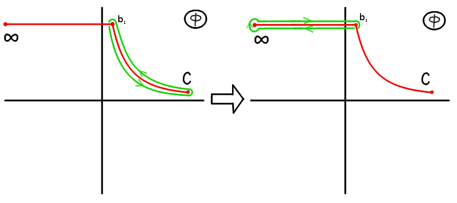
Figure 6: Deformation of integration contour in (30).

The integration contour ${\mathcal{C}}$ and its deformation are shown in fig. 6. Using the density in (12) with $\kappa=\mu=0$, the first integral in (30) can be deformed out to infinity and expressed as

$$\frac{kN\pi}{3}\int_{\mathcal{C}}\phi^{3}\rho(\phi)d\phi = \frac{N^{2}\pi^{2}}{6\tilde{\lambda}^{2}}\left(\frac{i}{2\pi}\right)\oint_{\infty}\phi^{3}\sqrt{\phi^{4}-\frac{4\tilde{\lambda}}{\pi}\phi+B}$$ (110)

$$= \frac{N^{2}\pi^{2}}{6\tilde{\lambda}^{2}}\left(\frac{i}{2\pi}\right)\oint_{\infty}\phi^{5}\left(1-\frac{2\tilde{\lambda}}{\pi}\phi^{-3}+\frac{B}{2}\phi^{-4}-\frac{2\tilde{\lambda}^{2}}{\pi^{2}}\phi^{-6}+\dots\right)$$

$$= \frac{N^{2}}{3}\,,$$

which is independent of $B$.

In the second term we can deform one of integration contours as shown on Fig.6, so that we get

$$-\frac{N^{2}}{2}\int_{\mathcal{C}}d\phi d\phi^{\prime}\rho(\phi)\rho(\phi^{\prime})\log(\phi-\phi^{\prime})^{2}$$

$$=-\frac{2\pi iN^{2}}{2}\int_{-\infty}^{b_{1}}\rho(\phi)d\phi\int_{\mathcal{C}_{1}}\rho(\phi^{\prime})d\phi^{\prime}-\frac{2\pi iN^{2}}{2}\int_{-\infty}^{b_{2}}\rho(\phi)d\phi\int_{\mathcal{C}_{2}}\rho(\phi^{\prime})d\phi^{\prime}$$

$$\qquad-\frac{N^{2}}{4}\oint_{\infty}\rho(\phi)\log\phi^{2}+\frac{N^{2}}{2}\oint_{\infty}\phi^{-3}\rho(\phi)d\phi\,\frac{1}{3}\int_{\mathcal{C}}{\phi^{\prime}}^{3}\rho(\phi^{\prime})d\phi^{\prime}\,,$$ (111)

where $\mathcal{C}_{1}$ and $\mathcal{C}_{2}$ refer to the two contours of eigenvalues and $b_{1}$ and $b_{2}$ are branch points on those contours. The first integral on the second line is assumed to start and stop at $-\infty$. For any value of $B$ we have that

$$-\frac{N^{2}}{4}\oint_{\infty}\rho(\phi)\log\phi^{2} = N^{2}\lim_{\phi\to-\infty}\left(-\frac{\pi}{6\tilde{\lambda}}|\phi|^{3}-\log|\phi|\right)$$

$$\frac{N^{2}}{2}\oint_{\infty}\phi^{-3}\rho(\phi)d\phi\,\frac{1}{3}\int_{\mathcal{C}}{\phi^{\prime}}^{3}\rho(\phi^{\prime})d\phi^{\prime} = \frac{N^{2}}{2}\frac{i}{2\tilde{\lambda}}\oint_{\infty}\frac{\phi^{2}d\phi}{\phi^{3}}\frac{\tilde{\lambda}}{3\pi}=-\frac{N^{2}}{6}\,.$$ (112)

For the other integrals we will consider special cases. Note that the $\phi^{\prime}$ integrals give the filling fractions for the contours. For the $Z_{3}$ solution which has $B=0$, we can treat the problem as having only one contour since the two contours actually touch at the origin. We then find that

$$-\frac{2\pi iN^{2}}{2}\int_{-\infty}^{b_{1}}\rho(\phi)d\phi = \lim_{\phi\to-\infty}N^{2}\Bigg{(}\frac{\pi}{6\tilde{\lambda}}|\phi|^{3}+\frac{\pi}{2\tilde{\lambda}}\frac{2}{3}\frac{\tilde{\lambda}}{\pi}(1+\log(4)+3\log(\phi))$$ (113)

$$\qquad\qquad\qquad\qquad\qquad+\frac{2\pi}{4\tilde{\lambda}}\left(-\frac{2\tilde{\lambda}}{3\pi}\right)\log\left(\frac{4\tilde{\lambda}}{\pi}\right)\Bigg{)}$$

$$= \lim_{\phi\to-\infty}N^{2}\left(\frac{\pi}{6\tilde{\lambda}}|\phi|^{3}+\log|\phi|+\frac{1}{3}-\frac{1}{3}\log\frac{\tilde{\lambda}}{\pi}\right)$$

For $B=-3\left({\pi}/{\tilde{\lambda}}\right)^{4/3}$ there is a single cut with a branch point at $\phi=\left(-1+i\sqrt{2}\right)\left({\tilde{\lambda}}/{\pi}\right)^{1/3}$. In this case we find

$$-\frac{2\pi iN^{2}}{2}\int_{-\infty}^{b_{1}}\rho(\phi)d\phi=\lim_{\phi\to-\infty}N^{2}\left(\frac{\pi}{6\tilde{\lambda}}|\phi|^{3}+\log|\phi|+\frac{1}{3}-\frac{1}{3}\log\frac{\tilde{\lambda}}{\pi}+\frac{1}{2}\log 2\right)\,.$$ (114)

Finally let us consider the cases with $B^{\pm}=-{3}\left({\pi}/{\tilde{\lambda}}\right)^{4/3}e^{\pm 2\pi i/3}$, corresponding to $Z_{3}$-rotations of the previous solution. It is clear that under the change of variables $\phi^{\prime}=e^{\mp 2\pi i/3}\phi$ that

$$-\frac{2\pi iN^{2}}{2}\int_{-\infty}^{b^{\pm}_{1}}\rho^{\pm}(\phi)d\phi=\lim_{|\phi|\to\infty}-\frac{2\pi iN^{2}}{2}\int_{-|\phi|e^{\mp 2\pi i/3}}^{b_{1}}\rho(\phi^{\prime})\,d\phi^{\prime}$$ (115)

where $\rho(\phi)$ and $b_{1}$ are the same as as in (114). Since the integral only depends on the absolute value of $\phi$ and not its phase, the result is the same as in (114). Thus the free energy is the same for all three single-cut solutions.

Combining (B) with (113) or (114) we find

$$-\frac{N^{2}}{2}\int_{\mathcal{C}}d\phi d\phi^{\prime}\rho(\phi)\rho(\phi^{\prime})\log(\phi-\phi^{\prime})^{2}$$

$$\qquad\qquad=N^{2}\left(\frac{1}{6}-\frac{1}{3}\log\frac{\tilde{\lambda}}{\pi}\right),\qquad\qquad B=0$$

$$\qquad\qquad=N^{2}\left(\frac{1}{6}-\frac{1}{3}\log\frac{\tilde{\lambda}}{\pi}+\frac{1}{2}\log 2\right),\quad B=-{3}\left(\frac{\pi}{\tilde{\lambda}}\right)^{4/3}e^{2\pi in/3}\,.$$ (116)

Therefore,

$$F = N^{2}\left(\frac{1}{2}-\frac{1}{3}\log\frac{\tilde{\lambda}}{\pi}-C\right)\qquad\qquad\qquad B=0$$

$$F = N^{2}\left(\frac{1}{2}-\frac{1}{3}\log\frac{\tilde{\lambda}}{\pi}+\frac{1}{2}\log 2-C\right)\qquad B=-{3}\left(\frac{\pi}{\tilde{\lambda}}\right)^{4/3}e^{2\pi in/3}\,.$$ (117)

Appendix C Exact solutions for $m^{2}=-1/4$

In this appendix we describe an exact single-cut solution to the full matrix model at the special value $m^{2}=-1/4$. As we emphasized in the main text, while the eigenvalues lying along the real axis are exponentially close to the exact solution for the strongly coupled pure CS model, the profile for those along the imaginary axis is not as clear because the approximations we assume in the solution break down near the imaginary axis. Furthermore, the numerical results show that while the eigenvalues are close to the imaginary axis, they appear scattered about it. Therefore, it is very useful to study any available exact solution to get a better picture of these structures.

At $m^{2}=-1/4$ the determinant of the partition function drastically simplifies and the pure CS eigenvalue equations reduce to

$$\frac{\pi N}{\tilde{\lambda}}\phi^{2}_{i} = 2\pi\sum\limits_{j\neq i}\coth(\pi(\phi_{i}-\phi_{j}))\,.$$ (118)

Defining the new variables $u_{i}=e^{2\pi\phi_{i}}$, we can put (118) into the standard form

$$\frac{N}{2}V^{\prime}(u_{i})=\sum\limits_{j\neq i}\frac{1}{u_{i}-u_{j}}\,,$$ (119)

where

$$V(u)=\frac{1}{24\pi^{2}\tilde{\lambda}}(\log u)^{3}+\log u\,.$$ (120)

In the large $N$ limit, a single cut solution will then have the eigenvalue density

$$\rho(u)=-\frac{1}{\pi^{2}}\sqrt{(a-u)(u-b)}\int^{a}_{b}\!\!\!\!\!\!\!\!\!-\frac{du^{\prime}}{(u-u^{\prime})\sqrt{(a-u^{\prime})(u^{\prime}-b)}}\frac{1}{2}V^{\prime}(u^{\prime})$$ (121)

where the end-points $a$ and $b$ are to be determined. The resolvent is then defined as

$$w(u)=\int_{b}^{a}\frac{\rho(u^{\prime})du^{\prime}}{u-u^{\prime}}\to\frac{1}{u}\ \mbox{as}\ u\to\infty\,.$$ (122)

Consistency with the equations of motion and the large $u$ behavior of the resolvent then leads to the following constraint equations

$$\int_{b}^{a}\frac{du}{\sqrt{(a-u)(u-b)}}\frac{1}{2}V^{\prime}(u) = 0$$

$$\frac{1}{\pi}\int_{b}^{a}\frac{du}{\sqrt{(a-u)(u-b)}}\frac{1}{2}V^{\prime}(u)u = 1\,,$$ (123)

giving us two complex equations for $a$ and $b$, and in principle making them determinable. If we define $U(u)=V(u)-\log u$, then the equations take the more symmetric form

$$\frac{\sqrt{ab}}{\pi}\int_{b}^{a}\frac{du}{\sqrt{(a-u)(u-b)}}U^{\prime}(u) = -1$$

$$\frac{1}{\pi}\int_{b}^{a}\frac{du}{\sqrt{(a-u)(u-b)}}U^{\prime}(u)u = +1\,,$$ (124)

The integrals can be done by first assuming that $a>b>0$ and then analytically continuing into the complex plane. In the first integral, by deforming the contour as demonstrated in Fig. 7, we can show that

$$\int_{b}^{a}\frac{(\log u)^{2}du}{u\sqrt{(a-u)(u-b)}}=\frac{1}{\sqrt{ab}}\left(\pi(\log(-u))^{2}\Bigg{|}_{{u\to 0_{-}}}\!\!\!-\frac{\pi^{3}}{3}\right)-2\pi\int_{-\infty}^{0_{-}}\frac{\log(-u)du}{u\sqrt{(a-u)(b-u)}}\,.$$

Integrating by parts, the integral on the rhs becomes

$$\frac{4\pi}{\sqrt{ab}}\log(-u)\,\mbox{arctanh}\left(\sqrt{\frac{b}{a}}\sqrt{\frac{a-u}{b-u}}\right)\Bigg{|}_{-\infty}^{0_{-}}-\frac{4\pi}{\sqrt{ab}}\int_{-\infty}^{0_{-}}\frac{du}{u}\mbox{arctanh}\left(\sqrt{\frac{b}{a}}\sqrt{\frac{a-u}{b-u}}\right)\,.$$ (126)

Letting $d=\sqrt{\frac{a}{b}}$ and defining $y=\sqrt{\frac{a-u}{b-u}}$, the last integral can be written as

$$-\frac{4\pi}{\sqrt{ab}}\int_{-\infty}^{0_{-}}\frac{du}{u}\mbox{arctanh}\left(\sqrt{\frac{b}{a}}\sqrt{\frac{a-u}{b-u}}\right)=\frac{2\pi}{\sqrt{ab}}(d^{2}-1)\int_{1}^{d}\frac{2ydy}{(d^{2}-y^{2})(y^{2}-1)}\log\frac{d+y}{d-y}\,.$$

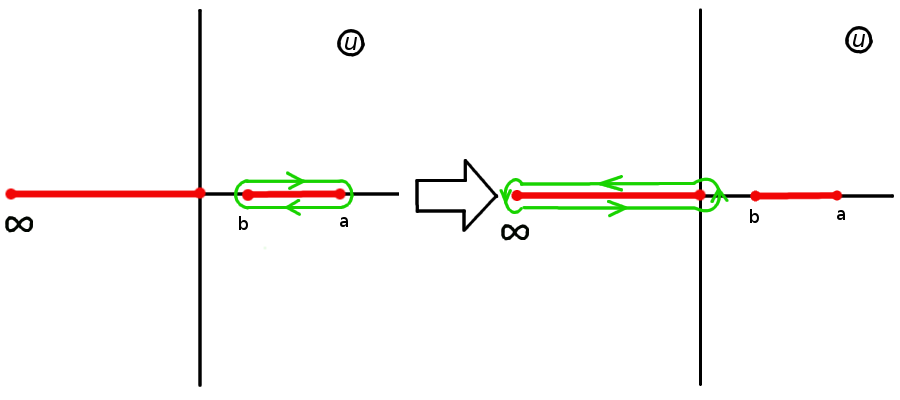
Figure 7: Deformation of the integration contour in (C).

This integral is solvable, where we find

$$\frac{2\pi}{\sqrt{ab}}(d^{2}-1)\int_{1}^{d}\frac{2y\,dy}{(d^{2}-y^{2})(y^{2}-1)}\log\frac{d+y}{d-y}=$$

$$\qquad\qquad\frac{2\pi}{\sqrt{ab}}\Bigg{(}\frac{\pi^{2}}{6}+\frac{1}{2}(\log(2d))^{2}-(\log(d-1))^{2}+(\log(d+1))^{2}-\log\frac{d+1}{d-1}\log(2d)$$

$$\qquad+\mbox{Li}_{2}\left(-\frac{2}{d-1}\right)-\mbox{Li}_{2}\left(\frac{d-1}{2d}\right)+\mbox{Li}_{2}\left(\frac{d-1}{d+1}\right)+\mbox{Li}_{2}\left(\frac{d+1}{2d}\right)$$

$$\qquad+\frac{1}{2}(\log(d-y))^{2}-\log(2d)\log(d-y)\Bigg{|}_{y\to d}-\log\frac{d+1}{d-1}\log(y-1)\Bigg{|}_{y\to 1}\Bigg{)}\,.$$ (128)

Combining all terms, the divergences cancel and using several dilogarithm identities, we find

$$\frac{\sqrt{ab}}{\pi}\int_{b}^{a}\frac{du}{\sqrt{(a\!-\!u)(u\!-\!b)}}U^{\prime}(u)=\frac{1}{4\pi^{2}\tilde{\lambda}}\left[\frac{1}{2}\left(\log(b)+2\log\frac{2d}{d\!+\!1}\right)^{2}+\mbox{Li}_{2}\left(\left(\frac{d\!-\!1}{d\!+\!1}\right)^{2}\right)\right]\,.$$

(129)

Using similar techniques, one can also show that

$$\frac{1}{\pi}\int_{b}^{a}\frac{du}{\sqrt{(a\!-\!u)(u\!-\!b)}}U^{\prime}(u)u=\frac{1}{4\pi^{2}\tilde{\lambda}}\left[\frac{1}{2}\left(\log(a)-2\log\frac{2d}{d\!+\!1}\right)^{2}+\mbox{Li}_{2}\left(\left(\frac{d\!-\!1}{d\!+\!1}\right)^{2}\right)\right]\,.$$

Hence, the conditions in (C) can be reexpressed as

$$\frac{1}{2}\left(\log(b)+2\log\frac{2d}{d+1}\right)^{2}+\mbox{Li}_{2}\left(\left(\frac{d-1}{d+1}\right)^{2}\right) = -4\pi^{2}\tilde{\lambda}$$

$$\frac{1}{2}\left(\log(a)-2\log\frac{2d}{d+1}\right)^{2}+\mbox{Li}_{2}\left(\left(\frac{d-1}{d+1}\right)^{2}\right) = +4\pi^{2}\tilde{\lambda}\,.$$ (131)

These equations can be rewritten in terms of the $\phi$ variables as

$$\left(\frac{4\pi^{2}\tilde{\lambda}}{Z}\right)^{2}+Z^{2}+2\,\mbox{Li}_{2}\left(1-e^{-Z}))\right) = 0$$

$$\phi_{max}+\phi_{min} = \frac{4\pi\tilde{\lambda}}{Z}$$ (132)

where $a=e^{2\pi\phi_{max}}$, $b=e^{2\pi\phi_{min}}$, and $Z=2\log(\cosh\frac{\pi}{2}(\phi_{max}-\phi_{min}))$

We can also derive an expression for the eigenvalue density $\rho(u)$. Using the identity

$$\frac{1}{u-u^{\prime}}=\frac{u^{\prime}}{u}\left(\frac{1}{u-u^{\prime}}+\frac{1}{u^{\prime}}\right)$$ (133)

and the first equation in (C), (121) can be rewritten as

$$\rho(u)=-\frac{1}{\pi^{2}}\frac{\sqrt{(a-u)(u-b)}}{u}\int^{a}_{b}\!\!\!\!\!\!\!\!\!-\frac{du^{\prime}}{(u-u^{\prime})\sqrt{(a-u^{\prime})(u^{\prime}-b)}}\frac{1}{2}V^{\prime}(u^{\prime})u^{\prime}\,.$$ (134)

The constant piece in $V^{\prime}(u^{\prime})u^{\prime}$ does not contribute to the integral. Deforming the contour to encircle the log branch cut, we then have

$$\rho(u)=\frac{1}{8\pi^{3}\tilde{\lambda}}\frac{\sqrt{(a-u)(u-b)}}{u}\int_{-\infty}^{0}\frac{\log(-u^{\prime})du^{\prime}}{(u-u^{\prime})\sqrt{(a-u^{\prime})(b-u^{\prime})}}\,.$$ (135)

Integrating by parts as in (126) and using the same substitutions of variables as in (126)-(129), we find

$$\rho(u) = \frac{i}{16\pi^{3}\tilde{\lambda}}\,\frac{1}{u}\Bigg{[}4\,\mbox{Li}_{2}\left(-\frac{1-y}{1+y}\right)+4\,\mbox{Li}_{2}\left(-\frac{1+y}{d-y}\right)-4\,\mbox{Li}_{2}\left(-\frac{1-y}{d+y}\right)-4\,\mbox{Li}_{2}\left(-\frac{d+y}{d-y}\right)$$ (136)

$$\qquad\qquad\quad+2\log b\left(\log\frac{d+y}{d-y}-\log\frac{1+y}{1-y}\right)+\left(\log\frac{d+y}{d-y}-\log\frac{1+y}{1-y}\right)^{2}$$

$$\qquad\qquad\quad-2\left(\log\frac{d-y}{1-y}\right)^{2}+2\left(\log\frac{d-y}{1+y}\right)^{2}-2\left(\log\frac{d+y}{d-y}\right)^{2}\Bigg{]}\,.$$

The endpoints are at $y=0,\infty$, with the distribution crossing over branch cuts from the logs and dilogarithms.

We first check these results for $\tilde{\lambda}\ll 1$. In this limit the end points in (121) approach $a=b=1$. Expanding about $d=1$ we find

$$\rho(\phi)=2\pi u\rho(u) \approx \frac{i}{8\pi^{2}\tilde{\lambda}}\frac{y(d-1)}{y^{2}-1}\left(2\log b+(d-1)-2\,\frac{d-1}{y^{2}-1}\right)$$ (137)

$$\approx \frac{1}{2\tilde{\lambda}}\left(\phi+\frac{1}{2}(\phi_{max}+\phi_{min})\right)\sqrt{(\phi_{max}-\phi)(\phi-\phi_{min})}\,,$$

which agrees with the density extracted from (11).

Let us now analyze our results in the limit of large $\tilde{\lambda}$. In this limit we assume that $|d|\gg 1$, justifying this afterwards. In this case the equations in (C) reduce to

$$\log(b)\approx 2\pi i\sqrt{2(\tilde{\lambda}+1/24)}-2\log 2\qquad\log(a)\approx 2\pi\sqrt{2(\tilde{\lambda}-1/24)}+2\log 2\,.$$ (138)

In terms of the $\phi$ variable this translates to

$$\phi_{min}\approx i\sqrt{2(\tilde{\lambda}+1/24)}-\frac{1}{\pi}\log 2\qquad\phi_{max}\approx\sqrt{2(\tilde{\lambda}-1/24)}+\frac{1}{\pi}\log 2\,.$$ (139)

Note that this is consistent to leading order in $\tilde{\lambda}$ with the endpoints in (38). We can also see that with these solutions

$$|d|=\bigg{|}\sqrt{\frac{a}{b}}\bigg{|}\approx 4\exp\left(\pi\sqrt{2(\tilde{\lambda}-1/24)}\right)\,,$$ (140)

showing that our approximations are accurate up to exponentially small corrections.

For large $\tilde{\lambda}$ we expect half the eigenvalues to extend along the positive real direction. In this region of the complex $\phi$ plane we have $|d|\gg|y|\gg 1$, except very close to the endpoint where $y\to 0$. Away from this endpoint the density in (136) is approximately

$$\rho(\phi)=2\pi u\rho(u) \approx \frac{i}{8\pi^{2}\tilde{\lambda}}\left(4\left(\frac{\pi^{2}}{6}+0-0-\left(-\frac{\pi^{2}}{12}\right)\right)+(-\pi i)^{2}\right.$$ (141)

$$\left.-2\pi i\log b-2\log\left(-\frac{d^{2}}{y^{2}}\right)\pi i\right)\approx\frac{1}{2\tilde{\lambda}}\phi\,,$$

which agrees with (36).

The analysis along the imaginary axis is trickier. In this case we have that $|y|,|d|\gg 1$, but which of these is bigger depends on the position along the distribution. It is convenient to define $z=d/y=\sqrt{\frac{1-u/b}{1-u/a}}$. The density can then be well-approximated by

$$\rho(\phi) \approx \frac{i}{8\pi^{2}\tilde{\lambda}}\Bigg{(}\left(2\log b+\log(4(1-z^{2}))\right)\log\frac{1+z}{1-z}$$ (142)

$$\qquad\qquad+2\mbox{Li}_{2}\left(\frac{1+z}{2}\right)-2\mbox{Li}_{2}\left(\frac{1-z}{2}\right)\Bigg{)}\,,$$

up to exponentially small corrections. It is obvious that this is an odd function of $z$. Furthermore, this can be integrated to give the relatively simple form

$$n(w) = \int_{\phi_{min}}^{\phi}\rho(\phi)d\phi$$

$$= \frac{i}{16\pi^{3}\tilde{\lambda}}\Bigg{(}\frac{1}{3}(\log(1-w)-\log w)[\pi^{2}-(\log w)^{2}-4\log w\log(1-w)-(\log(1-w))^{2}]$$

$$\qquad\qquad+4\,\mbox{Li}_{3}(w)-4\,\mbox{Li}_{3}(1-w)$$

$$\qquad+\log(4b)\Big{(}(\log w)^{2}-(\log(1-w))^{2}+2\mbox{Li}_{2}(w)-2\mbox{Li}_{2}(1-w)\Big{)}\Bigg{)}\,,$$

where $w=\frac{1+z}{2}$. $n(w)$ has cuts extending from 1 to $+\infty$ and from $0$ to $-\infty$, and the allowed $w$ on the eigenvalue path are chosen so that $n(w)$ is positive real. The eigenvalue path follows a contour that alternates crossing the negative branch cut from the bottom and the positive branch cut from the top (see for example fig. 8). If we follow a path such that we cross each cut $m$ times and return to the same value of $w$, then $n(w)$ shifts by

$$n(w)\to n(w)-\frac{1}{\tilde{\lambda}}\left(m^{2}+\frac{m\,i}{2\pi}\log(4b(w-w^{2}))\right)\,,$$ (144)

where $w$ is evaluated on the principle sheet. In terms of $\phi$ we can rewrite the shift as

$$n(w)\to n(w)+\frac{m}{\tilde{\lambda}}\left(m-{i\,}\phi\right)\,,$$ (145)

where under the transformation $\phi\to\phi-2im$.

We can now argue using (144) that a single contour is not a viable solution for large $\tilde{\lambda}$. If we are in the principle branch near the beginning of the contour then $n(w)$ is approximately

$$n(w)=-\frac{4\,i\,\log(4b)}{3\tilde{\lambda}\pi^{3}}(w-1/2)^{3}+{\rm O}((w-1/2)^{5})\,.$$ (146)

The three possible choices of contours originating out of the point $w=1/2$ are shown in fig. 8. Along these contours $n(w)$ is positive and increasing. One of the contours heads directly to the branch point at $w=1$, which corresponds to the undesired behavior of $\mbox{Re}(\phi)$ going to negative infinity.

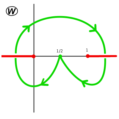
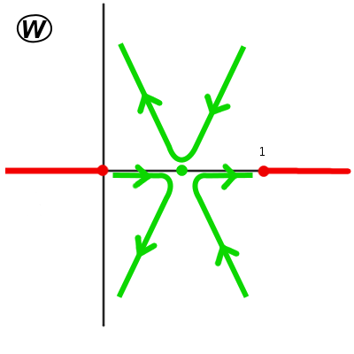
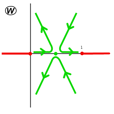
Figure 8: Path of the cut in $w$-plane.

Instead we should choose the contour that leads to the path shown in fig. 8 as we move away from $w=1/2$. In this case the contour will cross both branch cuts and start heading toward the $w=1/2$ point, but now in the $m=1$ branch. Near this point we should still insist that $n(w)$ is positive and increasing. Using the expansion in (146) and the shift in (144) we find that

$$n(w) \approx -\frac{4\,i\,\log(4b)}{3\tilde{\lambda}\pi^{3}}(w-1/2)^{3}-\frac{i}{2\pi\tilde{\lambda}}\log(b)-\frac{1}{\tilde{\lambda}}+\frac{2i}{\pi\tilde{\lambda}}(w-1/2)^{2}$$ (147)

$$\approx \frac{8\sqrt{2}}{3\sqrt{\tilde{\lambda}}\pi^{2}}(w-1/2)^{3}+\frac{\sqrt{2}}{\sqrt{\tilde{\lambda}}}+\frac{i\log(2)}{\pi\tilde{\lambda}}-\frac{1}{\tilde{\lambda}}+\frac{2i}{\pi\tilde{\lambda}}(w-1/2)^{2}\,,$$

with $w$ chosen so that the imaginary part in (147) is zero. Fig.8 shows the contours near $w=1/2$ that satisfy this condition. As can be seen, the contour that heads toward $w=1/2$ on Fig.8, makes a sharp turn near $w=1/2$ and heads toward the $w=1$ branch point, signifying the breakdown of the single cut solution.

This last analysis assumes that $\tilde{\lambda}$ is real. If instead we allow for a small imaginary part, then we can change the behavior in Fig.8. For example, let $\tilde{\lambda}=\rho e^{i\theta}$ where $\theta$ is assumed to be a small angle. Then for the $m^{\rm th}$ branch (147) becomes

$$n(w)\approx\frac{8\sqrt{2}}{3\sqrt{\rho}\pi^{2}}(w-1/2)^{3}+\frac{m}{\rho}(\sqrt{2\rho}-m)-i\frac{m}{2\rho}\theta(\sqrt{2\rho}-2m)+\frac{i\log(2)}{\pi\rho}+\frac{2im}{\pi\rho}(w-1/2)^{2}\,.$$

If we then have $\theta>\frac{2\log(2)}{\pi(\sqrt{2\rho}-2m)}$ then the contour will behave like fig. 8, at least for small enough $m$, allowing the contour to continue onto the next branch. However, as $m$ approaches $\sqrt{\rho/2}$ then the approximation starts breaking down.

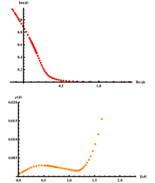
(a) $\tilde{\lambda}=0.8$

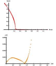
(b) $\tilde{\lambda}=0.976$

Figure 9: Cut behavior for different $\tilde{\lambda}$

Our interpretation of these results is that for large real $\tilde{\lambda}$ the contour likely splits into order $\sqrt{2\tilde{\lambda}}/2$ separate contours, with each contour roughly between the $w=1/2$ points of successive branches. This should at least be true for relatively small values of $m$. Since the densities are higher for the small values of $m$, these branches will dominate over the larger values. If we then give a small imaginary part to $\tilde{\lambda}$, then we expect the contours in the smaller $m$ regions to join together. The number of joined contours will increase as we increase $\theta$.

This also suggests that for real $\tilde{\lambda}$ there will be a succession of phase transitions as $\tilde{\lambda}$ is increased, with a transition every time $\sqrt{2\tilde{\lambda}}$ increases by $2$. Numerically we have found that starting at weak coupling, the single contour degenerates at $\tilde{\lambda}=\tilde{\lambda}_{c}\approx.976$. The behavior of the cut is shown in fig. 9. As we see from fig. 9(b), as $\tilde{\lambda}\to\tilde{\lambda}_{c}$ the density $\rho(\phi)$ goes to zero in the middle of the cut, but still close to the real line. The cut then breaks in two above $\tilde{\lambda}_{c}$. As we increase $\tilde{\lambda}$ above $\tilde{\lambda}_{c}$ we expect the contour to split every time $\sqrt{2\tilde{\lambda}}$ increases by $2$

We can also investigate the single-cut solution where the end points are symmetric about the real axis. To this end we let $a=q\,e^{i\theta}$, $b=q\,e^{-i\theta}$, and so $d=e^{i\theta}$. Subtracting the first equation in (C) from the second we arrive at the relation

$$\log q\log\left(\cos\frac{\theta}{2}\right)=2\pi^{2}\tilde{\lambda}\,.$$ (149)

This shows that $q<1$, thus in the $\phi$ plane the real part of the end-points is less than zero. We also see that the rhs of (149) is positive real and so $\theta<\pi$, hence the end-points are in the strip $-\pi<\mbox{Im}(\phi)<\pi$. Using (149) and (C) we can express the coupling entirely in terms of $\theta$,

$$\tilde{\lambda}=-\frac{1}{\pi^{2}}\log\left(\cos\frac{\theta}{2}\right)\left[-\left(\log\left(\cos\frac{\theta}{2}\right)\right)^{2}-\frac{1}{2}\,\mbox{Li}_{2}\left(-\tan^{2}\frac{\theta}{2}\right)\right]^{1/2}\,,$$ (150)

and thus $q$ in terms of $\theta$,

$$\log q=-2\left[-\left(\log\left(\cos\frac{\theta}{2}\right)\right)^{2}-\frac{1}{2}\,\mbox{Li}_{2}\left(-\tan^{2}\frac{\theta}{2}\right)\right]^{1/2}\,.$$ (151)

In the large $\tilde{\lambda}$ limit one finds that $\theta\to\pi$ and $\log q\to-\frac{\pi}{\sqrt{3}}$ up to exponentially small corrections. Therefore $a\to b$ and the endpoints of the cut approach $\phi=-\frac{1}{2\sqrt{3}}\pm\frac{i}{2}$.

To compute $\rho(u)$ we move slightly away from the limiting values and set $\theta=\pi-\epsilon$ in order to avoid potential divergences. The equations (150) and (151) then become

$$\tilde{\lambda}\approx-\frac{1}{2\sqrt{3}\pi}\log\frac{\epsilon}{2}\,,~{}~{}~{}~{}\log q\approx-\frac{\pi}{\sqrt{3}}-\frac{\sqrt{3}}{2\pi}\epsilon^{2}\log\epsilon\,.$$ (152)

We can use the first equation to rewrite the second as

$$\log q\approx-\frac{\pi}{\sqrt{3}}+3\,\tilde{\lambda}\,\epsilon^{2}\,.$$ (153)

The endpoints of the cut then take the form

$$\phi_{max}=-\frac{1}{2\sqrt{3}}+\frac{i}{2}-\frac{i\epsilon}{2\pi}\,,\hskip 22.76219pt\phi_{min}=-\frac{1}{2\sqrt{3}}-\frac{i}{2}+\frac{i\epsilon}{2\pi}\,.$$ (154)

Substituting these values into (136) we obtain

$$\rho(u)=-\frac{1}{2\pi u}\left(i+\frac{2\sqrt{3}\epsilon}{\pi}\right)\,,$$ (155)

or in terms of $\phi$,

$$\rho(\phi)=2\pi u\rho(u)=-i-\frac{2\sqrt{3}~{}\epsilon}{\pi}\,.$$ (156)

We determine the eigenvalue cut between the endpoints by setting

$$n(\phi)\equiv\int\limits_{\phi_{min}}^{\phi}\rho(\phi)~{}d\phi=-i\left(\phi+\frac{1}{2\sqrt{3}}+\frac{i}{2}\right)$$

to be positive real. Clearly this is true if we choose the cut to be parallel to the imaginary axis such that $\mbox{Re}(\phi)=-\frac{1}{2\sqrt{3}}$. In fig. 10 we show the numerical solution for $\tilde{\lambda}=50$, which confirms this behavior. Since this cut is of finite extent in the infinite $\tilde{\lambda}$ limit, the free-energy can only scale as $N^{2}$ and not $N^{5/2}$.

It is interesting to determine the behavior of the Wilson loop for this solution since it connects to the weakly coupled real single-cut solution in (62). Using the eigenvalue density in (156) and the endpoint positions in (154), we find that (54) gives for the log of the fundamental Wilson loop,

$$\log\langle W\rangle^{+}_{str.symm.}=-2\sqrt{3}\pi\tilde{\lambda}$$ (157)

This result parallels the decreasing behavior in (62). For other values of $m^{2}$, including $m^{2}=0$, we can show numerically that their Wilson loops are also decreasing with $\tilde{\lambda}$.

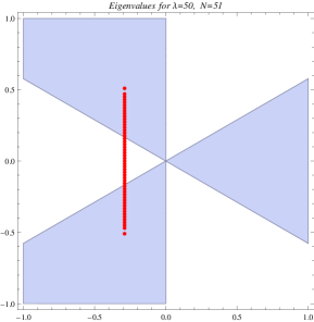
Figure 10: Numerical solution symmetric with respect to the real axis for $\tilde{\lambda}=50$.

References

- (1) E. Witten, String Theory Dynamics in Various Dimensions, Nucl.Phys. B443 (1995) 85–126, [hep-th/9503124].
- (2) N. Lambert, C. Papageorgakis, and M. Schmidt-Sommerfeld, M5-Branes, D4-Branes and Quantum 5D Super-Yang-Mills, JHEP 1101 (2011) 083, [arXiv:1012.2882].
- (3) M. R. Douglas, On D=5 super Yang-Mills theory and (2,0) theory, JHEP 1102 (2011) 011, [arXiv:1012.2880].
- (4) J. Kallen and M. Zabzine, Twisted supersymmetric 5D Yang-Mills theory and contact geometry, JHEP 1205 (2012) 125, [arXiv:1202.1956].
- (5) K. Hosomichi, R.-K. Seong, and S. Terashima, Supersymmetric Gauge Theories on the Five-Sphere, Nucl.Phys. B865 (2012) 376–396, [arXiv:1203.0371].
- (6) J. Kallen, J. Qiu, and M. Zabzine, The perturbative partition function of supersymmetric 5D Yang-Mills theory with matter on the five-sphere, arXiv:1206.6008.
- (7) H.-C. Kim and S. Kim, M5-branes from gauge theories on the 5-sphere, arXiv:1206.6339.
- (8) J. Kallen, J. Minahan, A. Nedelin, and M. Zabzine, -behavior from 5D Yang-Mills theory, JHEP 1210 (2012) 184, [arXiv:1207.3763].
- (9) J. A. Minahan, A. Nedelin, and M. Zabzine, 5D super Yang-Mills theory and the correspondence to AdS7/CFT6, J.Phys. A46 (2013) 355401, [arXiv:1304.1016].
- (10) I. R. Klebanov and A. A. Tseytlin, Entropy of Near Extremal Black P-Branes, Nucl.Phys. B475 (1996) 164–178, [hep-th/9604089].
- (11) M. Henningson and K. Skenderis, The Holographic Weyl Anomaly, JHEP 9807 (1998) 023, [hep-th/9806087].
- (12) J. Qiu and M. Zabzine, 5D Super Yang-Mills on Sasaki-Einstein Manifolds, arXiv:1307.3149.
- (13) N. Seiberg, Five-Dimensional SUSY Field Theories, Nontrivial Fixed Points and String Dynamics, Phys.Lett. B388 (1996) 753–760, [hep-th/9608111].
- (14) K. A. Intriligator, D. R. Morrison, and N. Seiberg, Five-Dimensional Supersymmetric Gauge Theories and Degenerations of Calabi-Yau Spaces, Nucl.Phys. B497 (1997) 56–100, [hep-th/9702198].
- (15) S. Ferrara, A. Kehagias, H. Partouche, and A. Zaffaroni, AdS(6) interpretation of 5-D superconformal field theories, Phys.Lett. B431 (1998) 57–62, [hep-th/9804006].
- (16) A. Brandhuber and Y. Oz, The D-4 - D-8 brane system and five-dimensional fixed points, Phys.Lett. B460 (1999) 307–312, [hep-th/9905148].
- (17) O. Bergman and D. Rodriguez-Gomez, 5d quivers and their AdS(6) duals, JHEP 1207 (2012) 171, [arXiv:1206.3503].
- (18) D. L. Jafferis and S. S. Pufu, Exact results for five-dimensional superconformal field theories with gravity duals, arXiv:1207.4359.
- (19) B. Assel, J. Estes, and M. Yamazaki, Wilson Loops in 5d N=1 SCFTs and AdS/CFT, arXiv:1212.1202.
- (20) P. Di Francesco, P. H. Ginsparg, and J. Zinn-Justin, 2-D Gravity and random matrices, Phys.Rept. 254 (1995) 1–133, [hep-th/9306153].
- (21) E. Brezin, C. Itzykson, G. Parisi, and J. Zuber, Planar Diagrams, Commun.Math.Phys. 59 (1978) 35.
- (22) E. Witten, Analytic Continuation of Chern-Simons Theory, arXiv:1001.2933.
- (23) G. Felder and R. Riser, Holomorphic Matrix Integrals, Nucl.Phys. B691 (2004) 251–258, [hep-th/0401191].
- (24) M. Marino, Lectures on non-perturbative effects in large N gauge theories, matrix models and strings, arXiv:1206.6272.
- (25) V. Pestun, Localization of Gauge Theory on a Four-Sphere and Supersymmetric Wilson Loops, Commun.Math.Phys. 313 (2012) 71–129, [arXiv:0712.2824].
- (26) H.-C. Kim, J. Kim, and S. Kim, Instantons on the 5-Sphere and M5-Branes, arXiv:1211.0144.
- (27) M. Marino, Lectures on localization and matrix models in supersymmetric Chern-Simons-matter theories, J.Phys.A A44 (2011) 463001, [arXiv:1104.0783].
- (28) C. P. Herzog, I. R. Klebanov, S. S. Pufu, and T. Tesileanu, Multi-Matrix Models and Tri-Sasaki Einstein Spaces, Phys.Rev. D83 (2011) 046001, [arXiv:1011.5487].
- (29) D. Young, Wilson Loops in Five-Dimensional Super-Yang-Mills, JHEP 1202 (2012) 052, [arXiv:1112.3309].
- (30) O. Bergman, D. Rodriguez-Gomez, and G. Zafrir, 5-Brane Webs, Symmetry Enhancement, and Duality in 5d Supersymmetric Gauge Theory, arXiv:1311.4199.
- (31) Y. Imamura and K. Kimura, On the moduli space of elliptic Maxwell-Chern-Simons theories, Prog.Theor.Phys. 120 (2008) 509–523, [arXiv:0806.3727].
- (32) O. Aharony, O. Bergman, D. L. Jafferis, and J. Maldacena, N=6 superconformal Chern-Simons-matter theories, M2-branes and their gravity duals, JHEP 0810 (2008) 091, [arXiv:0806.1218].
- (33) F. David, Planar Diagrams, Two-Dimensional Lattice Gravity and Surface Models, Nucl.Phys. B257 (1985) 45.
- (34) J. Ambjorn, B. Durhuus, and J. Frohlich, Diseases of Triangulated Random Surface Models, and Possible Cures, Nucl.Phys. B257 (1985) 433.
- (35) V. Kazakov, A. A. Migdal, and I. Kostov, Critical Properties of Randomly Triangulated Planar Random Surfaces, Phys.Lett. B157 (1985) 295–300.
- (36) D. Boulatov, V. Kazakov, I. Kostov, and A. A. Migdal, Analytical and Numerical Study of the Model of Dynamically Triangulated Random Surfaces, Nucl.Phys. B275 (1986) 641.
- (37) J. G. Russo and K. Zarembo, Evidence for Large-N Phase Transitions in * Theory, JHEP 1304 (2013) 065, [arXiv:1302.6968].
- (38) J. Russo and K. Zarembo, Massive Gauge Theories at Large N, JHEP 1311 (2013) 130, [arXiv:1309.1004].
- (39) A. Barranco and J. G. Russo, Large Phase Transitions in Supersymmetric Chern-Simons Theory with Massive Matter, JHEP 1403 (2014) 012, [arXiv:1401.3672].
- (40) J. G. Russo, G. A. Silva, and M. Tierz, Supersymmetric U(N) Chern-Simons-Matter Theory and Phase Transitions, arXiv:1407.4794.
- (41) L. Anderson and K. Zarembo, Quantum Phase Transitions in Mass-Deformed Abjm Matrix Model, arXiv:1406.3366.
- (42) F. David, Conformal Field Theories Coupled to 2D Gravity in the Conformal Gauge, Mod.Phys.Lett. A3 (1988) 1651.
- (43) E. Brezin and V. Kazakov, Exactly Solvable Field Theories of Closed Strings, Phys.Lett. B236 (1990) 144–150.
- (44) M. R. Douglas and S. H. Shenker, Strings in Less Than One-Dimension, Nucl.Phys. B335 (1990) 635.
- (45) D. J. Gross and A. A. Migdal, Nonperturbative Two-Dimensional Quantum Gravity, Phys.Rev.Lett. 64 (1990) 127.