Convex Calibration Dimension for
Multiclass Loss Matrices

Abstract

We study consistency properties of surrogate loss functions for general multiclass learning problems, defined by a general multiclass loss matrix. We extend the notion of classification calibration, which has been studied for binary and multiclass 0-1 classification problems (and for certain other specific learning problems), to the general multiclass setting, and derive necessary and sufficient conditions for a surrogate loss to be calibrated with respect to a loss matrix in this setting. We then introduce the notion of convex calibration dimension of a multiclass loss matrix, which measures the smallest ‘size’ of a prediction space in which it is possible to design a convex surrogate that is calibrated with respect to the loss matrix. We derive both upper and lower bounds on this quantity, and use these results to analyze various loss matrices. In particular, we apply our framework to study various subset ranking losses, and use the convex calibration dimension as a tool to show both the existence and non-existence of various types of convex calibrated surrogates for these losses. Our results strengthen recent results of Duchi et al. (2010) and Calauzènes et al. (2012) on the non-existence of certain types of convex calibrated surrogates in subset ranking. We anticipate the convex calibration dimension may prove to be a useful tool in the study and design of surrogate losses for general multiclass learning problems.

Keywords: Statistical consistency, multiclass loss, loss matrix, surrogate loss, convex surrogates, calibrated surrogates, classification calibration, subset ranking.

1 Introduction

There has been significant interest and progress in recent years in understanding consistency properties of surrogate risk minimization algorithms for various learning problems, such as binary classification, multiclass 0-1 classification, and various forms of ranking and multi-label prediction problems (Lugosi and Vayatis, 2004; Jiang, 2004; Zhang, 2004a; Steinwart, 2005; Bartlett et al., 2006; Zhang, 2004b; Tewari and Bartlett, 2007; Steinwart, 2007; Cossock and Zhang, 2008; Xia et al., 2008; Duchi et al., 2010; Ravikumar et al., 2011; Buffoni et al., 2011; Gao and Zhou, 2011; Kotlowski et al., 2011). Any such problem that involves a finite number of class labels and predictions can be viewed as an instance of a general multiclass learning problem, whose structure is defined by a suitable loss matrix. While the above studies have enabled an understanding of learning problems corresponding to certain forms of loss matrices, a framework for analyzing consistency properties for a general multiclass problem, defined by a general loss matrix, has remained elusive.

In this paper, we develop a unified framework for studying consistency properties of surrogate losses for such general multiclass learning problems, defined by a general multiclass loss matrix. For algorithms minimizing a surrogate loss, the question of consistency with respect to the target loss matrix reduces to the question of calibration of the surrogate loss with respect to the target loss. We start by giving both necessary and sufficient conditions for a surrogate loss function to be calibrated with respect to any given target loss matrix. These conditions generalize previous conditions for the multiclass 0-1 loss studied for example by Tewari and Bartlett (2007). We then introduce the notion of convex calibration dimension of a loss matrix, a fundamental quantity that measures the smallest ‘size’ of a prediction space in which it is possible to design a convex surrogate that is calibrated with respect to the given loss matrix. This quantity can be viewed as representing one measure of the intrinsic ‘difficulty’ of the loss, and has a non-trivial behavior in the sense that one can give examples of loss matrices defined on the same number of class labels that have very different values of the convex calibration dimension, ranging from one (in which case one can achieve consistency by learning a single real-valued function) to practically the number of classes (in which case one must learn as many real-valued functions as the number of classes). We give upper and lower bounds on this quantity in terms of various algebraic and geometric properties of the loss matrix, and apply these results to analyze various loss matrices.

As concrete applications of our framework, we use the convex calibration dimension as a tool to study various loss matrices that arise in subset ranking problems, including the normalized discounted cumulative gain (NDCG), pairwise disagreement (PD), and mean average precision (MAP) losses. A popular practice in subset ranking, where one needs to rank a set of $r$ documents by relevance to a query, has been to learn $r$ real-valued scoring functions by minimizing a convex surrogate loss in $r$ dimensions, and to then sort the $r$ documents based on these scores. As discussed recently by Duchi et al. (2010) and Calauzènes et al. (2012), such an approach cannot be consistent for the PD and MAP losses, since these losses do not admit convex calibrated surrogates in $r$ dimensions that can be used together with the sorting operation. We obtain a stronger result; in particular, we show that the convex calibration dimension of these losses is lower bounded by a quadratic function of $r$, which means that if minimizing a convex surrogate loss, one necessarily needs to learn $\Omega(r^{2})$ real-valued functions to achieve consistency for these losses.

1.1 Related Work

There has been much work in recent years on consistency and calibration of surrogate losses for various learning problems. We give a brief overview of this body of work here.

Initial work on consistency of surrogate risk minimization algorithms focused largely on binary classification. For example, Steinwart (2005) showed the consistency of support vector machines with universal kernels for the problem of binary classification; Jiang (2004) and Lugosi and Vayatis (2004) showed similar results for boosting methods. Bartlett et al. (2006) and Zhang (2004a) studied the calibration of margin-based surrogates for binary classification. In particular, in their seminal work, Bartlett et al. (2006) established that the property of ‘classification calibration’ of a surrogate loss is equivalent to its minimization yielding 0-1 consistency, and gave a simple necessary and sufficient condition for convex margin-based surrogates to be calibrated w.r.t. the binary 0-1 loss. More recently, Reid and Williamson (2010) analyzed the calibration of a general family of surrogates termed proper composite surrogates for binary classification. Variants of standard 0-1 binary classification have also been studied; for example, Yuan and Wegkamp (2010) studied consistency for the problem of binary classification with a reject option, and Scott (2012) studied calibrated surrogates for cost-sensitive binary classification.

Over the years, there has been significant interest in extending the understanding of consistency and calibrated surrogates to various multiclass learning problems. Early work in this direction, pioneered by Zhang (2004b) and Tewari and Bartlett (2007), considered mainly the multiclass 0-1 classification problem. This work generalized the framework of Bartlett et al. (2006) to the multiclass 0-1 setting and used these results to study calibration of various surrogates proposed for multiclass 0-1 classification, such as the surrogates of Weston and Watkins (1999), Crammer and Singer (2001), and Lee et al. (2004). In particular, while the multiclass surrogate of Lee et al. (2004) was shown to calibrated for multiclass 0-1 classification, it was shown that several other widely used multiclass surrogates are in fact not calibrated for multiclass 0-1 classification.

More recently, there has been much work on studying consistency and calibration for various other learning problems that also involve finite label and prediction spaces. For example, Gao and Zhou (2011) studied consistency and calibration for multi-label prediction with the Hamming loss. Another prominent class of learning problems for which consistency and calibration have been studied recently is that of subset ranking, where instances contain queries together with sets of documents, and the goal is to learn a prediction model that given such an instance ranks the documents by relevance to the query. Various subset ranking losses have been investigated in recent years. Cossock and Zhang (2008) studied subset ranking with the discounted cumulative gain (DCG) ranking loss, and gave a simple surrogate calibrated w.r.t. this loss; Ravikumar et al. (2011) further studied subset ranking with the normalized DCG (NDCG) loss. Xia et al. (2008) considered the 0-1 loss applied to permutations. Duchi et al. (2010) focused on subset ranking with the pairwise disagreement (PD) loss, and showed that several popular convex score-based surrogates used for this problem are in fact not calibrated w.r.t. this loss; they also conjectured that such surrogates may not exist. Calauzènes et al. (2012) showed conclusively that there do not exist any convex score-based surrogates that are calibrated w.r.t. the PD loss, or w.r.t. the mean average precision (MAP) or expected reciprocal rank (ERR) losses. Finally, in a more general study of subset ranking losses, Buffoni et al. (2011) introduced the notion of ‘standardization’ for subset ranking losses, and gave a way to construct convex calibrated score-based surrogates for subset ranking losses that can be ‘standardized’; they showed that while the DCG and NDCG losses can be standardized, the MAP and ERR losses cannot be standardized.

We also point out that in a related but different context, consistency of ranking has also been studied in the instance ranking setting (Clémençon and Vayatis, 2007; Clémençon et al., 2008; Kotlowski et al., 2011; Agarwal, 2014).

Finally, Steinwart (2007) considered consistency and calibration in a very general setting. More recently, Pires et al. (2013) used Steinwart’s techniques to obtain surrogate regret bounds for certain surrogates w.r.t. general multiclass losses, and Ramaswamy et al. (2013) showed how to design explicit convex calibrated surrogates for any low-rank loss matrix.

1.2 Contributions of this Paper

As noted above, we develop a unified framework for studying consistency and calibration for general multiclass (finite-output) learning problems, described by a general loss matrix. We give both necessary conditions and sufficient conditions for a surrogate loss to be calibrated w.r.t. a given multiclass loss matrix, and introduce the notion of convex calibration dimension of a loss matrix, which measures the smallest ‘size’ of a prediction space in which it is possible to design a convex surrogate that is calibrated with respect to the loss matrix. We derive both upper and lower bounds on this quantity in terms of certain algebraic and geometric properties of the loss matrix, and apply these results to study various subset ranking losses. In particular, we obtain stronger results on the non-existence of convex calibrated surrogates for certain types of subset ranking losses than previous results in the literature (and also positive results on the existence of convex calibrated surrogates for these losses in higher dimensions). The following is a summary of the main differences from the conference version of this paper (Ramaswamy and Agarwal, 2012):

• Enhanced definition of positive normal sets of a surrogate loss at a sequence of points (Definition 5; this is required for proofs of stronger versions of our earlier results).

• Stronger necessary condition for calibration (Theorem 7).

• Stronger versions of upper and lower bounds on the convex calibration dimension, with full proofs (Theorems 12, 16).

• Conditions under which the upper and lower bounds are tight (Section 4.3).

• Application to a more general setting of the PD loss (Section 5.2).

• Additional applications to the NDCG and MAP losses (Sections 5.1, 5.3).

• Additional examples and illustrations throughout (Examples 5, 6, 7, 9; Figures 3, 4).
  

• Minor improvements and changes in emphasis in notation and terminology.

1.3 Organization

We start in Section 2 with some preliminaries and examples that will be used as running examples to illustrate concepts throughout the paper, and formalize the notion of calibration with respect to a general multiclass loss matrix. In Section 3, we derive both necessary conditions and sufficient conditions for calibration with respect to general loss matrices; these are both of independent interest and useful in our later results. Section 4 introduces the notion of convex calibration dimension of a loss matrix and derives both upper and lower bounds on this quantity. In Section 5, we apply our results to study the convex calibration dimension of various subset ranking losses. We conclude with a brief discussion in Section 6. Shorter proofs are included in the main text; all longer proofs are collected in Section 7 so as to maintain easy readability of the main text. The only exception to this is proofs of Lemma 2 and Theorem 3, which closely follow earlier proofs of Tewari and Bartlett (2007) and are included for completeness in Appendix A. Some calculations are given in Appendices B and C.

2 Preliminaries, Examples, and Background

In this section we set up basic notation (Section 2.1), give background on multiclass loss matrices and risks (Section 2.2) and on multiclass surrogates and calibration (Section 2.3), and then define certain properties associated with multiclass losses and surrogates that will be useful in our study (Section 2.4).

2.1 Notation

Throughout the paper, we denote ${\mathbb{R}}=(-\infty,\infty)$, ${\mathbb{R}}_{+}=[0,\infty)$, $\overline{{\mathbb{R}}}=[-\infty,\infty]$, $\overline{{\mathbb{R}}}_{+}=[0,\infty]$. Similarly, ${\mathbb{Z}}$ and ${\mathbb{Z}}_{+}$ denote the sets of all integers and non-negative integers, respectively. For $n\in{\mathbb{Z}}_{+}$, we denote $[n]=\{1,\ldots,n\}$. For a predicate $\phi$, we denote by ${\mathbf{1}}(\phi)$ the indicator of $\phi$, which takes the value 1 if $\phi$ is true and 0 otherwise. For $z\in{\mathbb{R}}$, we denote $z_{+}=\max(0,z)$. For a vector ${\mathbf{v}}\in{\mathbb{R}}^{n}$, we denote $\|{\mathbf{v}}\|_{0}=\sum_{i=1}^{n}{\mathbf{1}}(v_{i}\neq 0)$ and $\|{\mathbf{v}}\|_{1}=\sum_{i=1}^{n}|v_{i}|$. For a set ${\mathcal{A}}\subseteq{\mathbb{R}}^{n}$, we denote by $\operatorname{relint}({\mathcal{A}})$ the relative interior of ${\mathcal{A}}$, by $\textup{{cl}}({\mathcal{A}})$ the closure of ${\mathcal{A}}$, by $\operatorname{span}({\mathcal{A}})$ the linear span (or linear hull) of ${\mathcal{A}}$, by $\textup{{aff}}({\mathcal{A}})$ the affine hull of ${\mathcal{A}}$, and by $\operatorname{conv}({\mathcal{A}})$ the convex hull of ${\mathcal{A}}$. For a vector space ${\mathcal{V}}$, we denote by $\operatorname{dim}({\mathcal{V}})$ the dimension of ${\mathcal{V}}$. For a matrix ${\mathbf{M}}\in{\mathbb{R}}^{m\times n}$, we denote by $\operatorname{rank}({\mathbf{M}})$ the rank of ${\mathbf{M}}$, by $\operatorname{affdim}({\mathbf{M}})$ the affine dimension of the set of columns of ${\mathbf{M}}$ (i.e. the dimension of the subspace parallel to the affine hull of the columns of ${\mathbf{M}}$), by $\textup{{null}}({\mathbf{M}})$ the null space of ${\mathbf{M}}$, and by $\operatorname{nullity}({\mathbf{M}})$ the nullity of ${\mathbf{M}}$ (i.e. the dimension of the null space of ${\mathbf{M}}$). We denote by $\Delta_{n}$ the probability simplex in ${\mathbb{R}}^{n}$: $\Delta_{n}=\{{\mathbf{p}}\in{\mathbb{R}}_{+}^{n}:\sum_{i=1}^{n}p_{i}=1\}$. Finally, we denote by $\Pi_{n}$ the set of all permutations of $[n]$, i.e. the set of all bijective mappings $\sigma:[n]{\rightarrow}[n]$; for a permutation $\sigma\in\Pi_{n}$ and element $i\in[n]$, $\sigma(i)$ therefore represents the position of element $i$ under $\sigma$.

2.2 Multiclass Losses and Risks

The general multiclass learning problem we consider can be described as follows: There is a finite set of class labels ${\mathcal{Y}}$ and a finite set of possible predictions $\widehat{{\mathcal{Y}}}$, which we take without loss of generality to be ${\mathcal{Y}}=[n]$ and $\widehat{{\mathcal{Y}}}=[k]$ for some $n,k\in{\mathbb{Z}}_{+}$. We are given training examples $(X_{1},Y_{1}),\ldots,(X_{m},Y_{m})$ drawn i.i.d. from a distribution $D$ on ${\mathcal{X}}\times{\mathcal{Y}}$, where ${\mathcal{X}}$ is an instance space, and the goal is to learn from these examples a prediction model $h:{\mathcal{X}}{\rightarrow}\widehat{{\mathcal{Y}}}$ which given a new instance $x\in{\mathcal{X}}$, makes a prediction $\widehat{y}=h(x)\in\widehat{{\mathcal{Y}}}$. In many common learning problems, the label and prediction spaces are the same, i.e.  $\widehat{{\mathcal{Y}}}={\mathcal{Y}}$, but in general, these could be different (e.g. when there is an ‘abstain’ option available to a classifier, in which case $k=n+1$).

The performance of a prediction model is measured via a loss function $\ell:{\mathcal{Y}}\times\widehat{{\mathcal{Y}}}{\rightarrow}{\mathbb{R}}_{+}$, or equivalently, by a loss matrix ${\mathbf{L}}\in{\mathbb{R}}_{+}^{n\times k}$, with $(y,t)$-th element given by $\ell_{yt}=\ell(y,t)$; here $\ell_{yt}=\ell(y,t)$ defines the penalty incurred on predicting $t\in[k]$ when the true label is $y\in[n]$. We will use the notions of loss matrix and loss function interchangeably. Some examples of common multiclass loss functions and corresponding loss matrices are given below:

Example 1 (0-1 loss)

Here ${\mathcal{Y}}=\widehat{{\mathcal{Y}}}=[n]$, and the loss incurred is $1$ if the predicted label $t$ is different from the actual class label $y$, and $0$ otherwise:

$$\ell^{\textup{{0-1}}}(y,t)~{}=~{}{\mathbf{1}}\big{(}t\neq y\big{)}~{}~{}~{}~{}~{}~{}~{}~{}\forall y,t\in[n]\,.$$

The loss matrix ${\mathbf{L}}^{\textup{{0-1}}}$ for $n=3$ is shown in Figure 1(a). This is one of the most commonly used multiclass losses, and is suitable when all prediction errors are considered equal.

Example 2 (Ordinal regression loss)

Here ${\mathcal{Y}}=\widehat{{\mathcal{Y}}}=[n]$, and predictions $t$ farther away from the actual class label $y$ are penalized more heavily, e.g. using absolute distance:

$$\ell^{\textup{{ord}}}(y,t)~{}=~{}|t-y|~{}~{}~{}~{}~{}~{}~{}~{}\forall y,t\in[n]\,.$$

The loss matrix ${\mathbf{L}}^{\textup{{ord}}}$ for $n=3$ is shown in Figure 1(b). This loss is often used when the class labels satisfy a natural ordinal property, for example in evaluating recommender systems that predict the number of stars (say out of 5) assigned to a product by user.

Example 3 (Hamming loss)

Here ${\mathcal{Y}}=\widehat{{\mathcal{Y}}}=[2^{r}]$ for some $r\in{\mathbb{Z}}_{+}$, and the loss incurred on predicting $t$ when the actual class label is $y$ is the number of bit-positions in which the $r$-bit binary representations of $t-1$ and $y-1$ differ:

$$\ell^{\textup{{Ham}}}(y,t)~{}=~{}\sum_{i=1}^{r}{\mathbf{1}}\big{(}(t-1)_{i}\neq(y-1)_{i}\big{)}~{}~{}~{}~{}~{}~{}~{}~{}\forall y,t\in[2^{r}]\,,$$

where for each $z\in\{0,\ldots,2^{r}-1\}$, $z_{i}\in\{0,1\}$ denotes the $i$-th bit in the $r$-bit binary representation of $z$. The loss matrix ${\mathbf{L}}^{\textup{{Ham}}}$ for $r=2$ is shown in Figure 1(c). This loss is frequently used in sequence learning applications, where each element in ${\mathcal{Y}}=\widehat{{\mathcal{Y}}}$ is a binary sequence of length $r$, and the loss in predicting a sequence ${\mathbf{t}}\in\{0,1\}^{r}$ when the true label sequence is ${\mathbf{y}}\in\{0,1\}^{r}$ is simply the Hamming distance between the two sequences.

Example 4 (‘Abstain’ loss)

Here ${\mathcal{Y}}=[n]$ and $\widehat{{\mathcal{Y}}}=[n+1]$, where $t=n+1$ denotes a prediction of ‘abstain’ (or ‘reject’). One possible loss function in this setting assigns a loss of $1$ to incorrect predictions in $[n]$, $0$ to correct predictions, and ${\frac{1}{2}}$ for abstaining:

$$\ell^{\textup{{(?)}}}(y,t)~{}=~{}{\mathbf{1}}\big{(}t\in[n]\big{)}\cdot{\mathbf{1}}\big{(}t\neq y\big{)}+\frac{1}{2}\cdot{\mathbf{1}}\big{(}t=n+1\big{)}~{}~{}~{}~{}~{}~{}~{}~{}\forall y\in[n],t\in[n+1]\,.$$

The loss matrix ${\mathbf{L}}^{\textup{{(?)}}}$ for $n=3$ is shown in Figure 1(d). This type of loss is suitable in applications where making an erroneous prediction is more costly than simply abstaining. For example, in medical diagnosis applications, when uncertain about the correct prediction, it may be better to abstain and request human intervention rather than make a misdiagnosis.

$${\underset{\textrm{\rule{0.0pt}{11.0pt}\normalsize{(a)}}}{\left[\begin{array}[]{ccc}0&1&1\\ 1&0&1\\ 1&1&0\end{array}\right]}}\hskip 14.22636pt{\underset{\textrm{\rule{0.0pt}{11.0pt}\normalsize{(b)}}}{\left[\begin{array}[]{ccc}0&1&2\\ 1&0&1\\ 2&1&0\end{array}\right]}}\hskip 14.22636pt{\underset{\textrm{\normalsize{(c)}}}{\left[\begin{array}[]{cccc}0&1&1&2\\ 1&0&2&1\\ 1&2&0&1\\ 2&1&1&0\end{array}\right]}}\hskip 14.22636pt{\underset{\textrm{\rule{0.0pt}{11.0pt}\normalsize{(d)}}}{\left[\begin{array}[]{cccc}0&1&1&{\frac{1}{2}}\\ 1&0&1&{\frac{1}{2}}\\ 1&1&0&{\frac{1}{2}}\\ \end{array}\right]}}$$

Figure 1: Loss matrices corresponding to Examples 1-4: (a) ${\mathbf{L}}^{\textup{{0-1}}}$ for $n=3$; (b) ${\mathbf{L}}^{\textup{{ord}}}$ for $n=3$; (c) ${\mathbf{L}}^{\textup{{Ham}}}$ for $r=2$ ($n=4$); (d) ${\mathbf{L}}^{\textup{{(?)}}}$ for $n=3$.

As noted above, given examples $(X_{1},Y_{1}),\ldots,(X_{m},Y_{m})$ drawn i.i.d. from a distribution $D$ on ${\mathcal{X}}\times[n]$, the goal is to learn a prediction model $h:{\mathcal{X}}{\rightarrow}[k]$. More specifically, given a target loss matrix ${\mathbf{L}}\in{\mathbb{R}}_{+}^{n\times k}$ with $(y,t)$-th element $\ell_{yt}$, the goal is to learn a model $h:{\mathcal{X}}{\rightarrow}[k]$ with small expected loss on a new example drawn randomly from $D$, which we will refer to as the ${\mathbf{L}}$-risk or ${\mathbf{L}}$-error of $h$:

$$\textup{{er}}_{D}^{\mathbf{L}}[h]~{}\stackrel{{\scriptstyle\triangle}}{{=}}~{}{\mathbf{E}}_{(X,Y)\sim D}\big{[}\ell_{Y,h(X)}\big{]}\,.$$ (1)

Clearly, denoting the $t$-th column of ${\mathbf{L}}$ as ${\boldsymbol{\ell}}_{t}=(\ell_{1t},\ldots,\ell_{nt})^{\top}\in{\mathbb{R}}_{+}^{n}$, and the class probability vector at an instance $x\in{\mathcal{X}}$ under $D$ as ${\mathbf{p}}(x)=(p_{1}(x),\ldots,p_{n}(x))^{\top}\in\Delta_{n}$, where $p_{y}(x)={\mathbf{P}}(Y=y\mid X=x)$ under $D$, the ${\mathbf{L}}$-risk of $h$ can be written as

$$\textup{{er}}_{D}^{\mathbf{L}}[h]~{}=~{}{\mathbf{E}}_{X}\bigg{[}\sum_{y=1}^{n}p_{y}(X)\,\ell_{y,h(X)}\bigg{]}~{}=~{}{\mathbf{E}}_{X}\Big{[}{\mathbf{p}}(X)^{\top}{\boldsymbol{\ell}}_{h(X)}\Big{]}\,.$$ (2)

The optimal ${\mathbf{L}}$-risk or optimal ${\mathbf{L}}$-error for a distribution $D$ is then simply the smallest ${\mathbf{L}}$-risk or ${\mathbf{L}}$-error that can be achieved by any model $h$:

$$\textup{{er}}^{{\mathbf{L}},*}_{D}~{}\stackrel{{\scriptstyle\triangle}}{{=}}~{}\inf_{h:{\mathcal{X}}{\rightarrow}[k]}\textup{{er}}^{{\mathbf{L}}}_{D}[h]~{}=~{}\inf_{h:{\mathcal{X}}{\rightarrow}[k]}{\mathbf{E}}_{X}\Big{[}{\mathbf{p}}(X)^{\top}{\boldsymbol{\ell}}_{h(X)}\Big{]}~{}=~{}{\mathbf{E}}_{X}\bigg{[}\min_{t\in[k]}\,{\mathbf{p}}(X)^{\top}{\boldsymbol{\ell}}_{t}\bigg{]}\,.$$ (3)

Ideally, one would like to minimize (approximately) the ${\mathbf{L}}$-risk, e.g. by selecting a model that minimizes the average ${\mathbf{L}}$-loss on the training examples among some suitable class of models. However, minimizing the discrete ${\mathbf{L}}$-risk directly is typically computationally difficult. Consequently, one usually minimizes a (convex) surrogate risk instead.

2.3 Multiclass Surrogates and Calibration

Let $d\in{\mathbb{Z}}_{+}$, and let ${\mathcal{C}}\subseteq{\mathbb{R}}^{d}$ be a convex set. A surrogate loss function $\psi:{\mathcal{Y}}\times{\mathcal{C}}{\rightarrow}{\mathbb{R}}_{+}$ acting on the surrogate prediction space ${\mathcal{C}}$ assigns a penalty $\psi(y,{\mathbf{u}})$ on making a surrogate prediction ${\mathbf{u}}\in{\mathcal{C}}$ when the true label is $y\in[n]$. The $\psi$-risk or $\psi$-error of a surrogate prediction model ${\mathbf{f}}:{\mathcal{X}}{\rightarrow}{\mathcal{C}}$ w.r.t. a distribution $D$ on ${\mathcal{X}}\times[n]$ is then defined as

$$\textup{{er}}^{\psi}_{D}[{\mathbf{f}}]~{}\stackrel{{\scriptstyle\triangle}}{{=}}~{}{\mathbf{E}}_{(X,Y)\sim D}\Big{[}\psi\big{(}Y,{\mathbf{f}}(X)\big{)}\Big{]}\,.$$ (4)

The surrogate $\psi$ can be represented via $n$ real-valued functions $\psi_{y}:{\mathcal{C}}{\rightarrow}{\mathbb{R}}_{+}$ for $y\in[n]$, defined as $\psi_{y}({\mathbf{u}})=\psi(y,{\mathbf{u}})\,;$ equivalently, we can also represent the surrogate $\psi$ as a vector-valued function ${\boldsymbol{\psi}}:{\mathcal{C}}{\rightarrow}{\mathbb{R}}_{+}^{n}$, defined as ${\boldsymbol{\psi}}({\mathbf{u}})=\big{(}\psi_{1}({\mathbf{u}}),\ldots,\psi_{n}({\mathbf{u}})\big{)}^{\top}\,.$ Clearly, the $\psi$-risk of ${\mathbf{f}}$ can then be written as

$$\textup{{er}}^{\psi}_{D}[{\mathbf{f}}]~{}=~{}{\mathbf{E}}_{X}\bigg{[}\sum_{y=1}^{n}p_{y}(X)\,\psi_{y}({\mathbf{f}}(X))\bigg{]}~{}=~{}{\mathbf{E}}_{X}\Big{[}{\mathbf{p}}(X)^{\top}{\boldsymbol{\psi}}({\mathbf{f}}(X))\Big{]}\,.$$ (5)

The optimal $\psi$-risk or optimal $\psi$-error for a distribution $D$ is then simply the smallest $\psi$-risk or $\psi$-error that can be achieved by any model ${\mathbf{f}}$:

$$\textup{{er}}^{\psi,*}_{D}~{}\stackrel{{\scriptstyle\triangle}}{{=}}~{}\inf_{{\mathbf{f}}:{\mathcal{X}}{\rightarrow}{\mathcal{C}}}\textup{{er}}^{\psi}_{D}[{\mathbf{f}}]~{}=~{}\inf_{{\mathbf{f}}:{\mathcal{X}}{\rightarrow}{\mathcal{C}}}{\mathbf{E}}_{X}\Big{[}{\mathbf{p}}(X)^{\top}{\boldsymbol{\psi}}({\mathbf{f}}(X))\Big{]}~{}=~{}{\mathbf{E}}_{X}\bigg{[}\inf_{{\mathbf{u}}\in{\mathcal{C}}}{\mathbf{p}}(X)^{\top}{\boldsymbol{\psi}}({\mathbf{u}})\bigg{]}\,.$$ (6)

We will find it convenient to define the sets

$${\mathcal{R}}_{\psi} \stackrel{{\scriptstyle\triangle}}{{=}} {\boldsymbol{\psi}}({\mathcal{C}})~{}\subseteq~{}{\mathbb{R}}_{+}^{n}$$ (7)

$${\mathcal{S}}_{\psi} \stackrel{{\scriptstyle\triangle}}{{=}} \operatorname{conv}({\mathcal{R}}_{\psi})~{}\subseteq~{}{\mathbb{R}}_{+}^{n}\,.$$ (8)

Clearly, the optimal $\psi$-risk can then also be written as

$$\textup{{er}}^{\psi,*}_{D}~{}=~{}{\mathbf{E}}_{X}\bigg{[}\inf_{{\mathbf{z}}\in{\mathcal{R}}_{\psi}}{\mathbf{p}}(X)^{\top}{\mathbf{z}}\bigg{]}~{}=~{}{\mathbf{E}}_{X}\bigg{[}\inf_{{\mathbf{z}}\in{\mathcal{S}}_{\psi}}{\mathbf{p}}(X)^{\top}{\mathbf{z}}\bigg{]}\,.$$ (9)

Example 5 (Crammer-Singer surrogate)

The Crammer-Singer surrogate was proposed as a hinge-like surrogate loss for 0-1 multiclass classification (Crammer and Singer, 2001). For ${\mathcal{Y}}=[n]$, the Crammer-Singer surrogate ${\boldsymbol{\psi}}^{\textup{{CS}}}$ acts on the surrogate prediction space ${\mathcal{C}}={\mathbb{R}}^{n}$ and is defined as follows:

$$\psi^{\textup{{CS}}}_{y}({\mathbf{u}})~{}=~{}\max_{y^{\prime}\in[n],y^{\prime}\neq y}\big{(}1-(u_{y}-u_{y^{\prime}})\big{)}_{+}~{}~{}~{}~{}~{}~{}~{}~{}\forall y\in[n],{\mathbf{u}}\in{\mathbb{R}}^{n}\,.$$

A surrogate ${\boldsymbol{\psi}}$ is convex if $\psi_{y}$ is convex $\forall y\in[n]$. As an example, the Crammer-Singer surrogate defined above is clearly convex. Given training examples $(X_{1},Y_{1}),\ldots,(X_{m},Y_{m})$ drawn i.i.d. from a distribution $D$ on ${\mathcal{X}}\times[n]$, a (convex) surrogate risk minimization algorithm using a (convex) surrogate loss ${\boldsymbol{\psi}}:{\mathcal{C}}{\rightarrow}{\mathbb{R}}_{+}^{n}$ learns a surrogate prediction model by minimizing (approximately, based on the training sample) the $\psi$-risk; the learned model ${\mathbf{f}}:{\mathcal{X}}{\rightarrow}{\mathcal{C}}$ is then used to make predictions in the original space $[k]$ via some transformation $\textup{{pred}}:{\mathcal{C}}{\rightarrow}[k]$. This yields a prediction model $h:{\mathcal{X}}{\rightarrow}[k]$ for the original multiclass problem given by $h=(\textup{{pred}}\circ{\mathbf{f}})$: the prediction on a new instance $x\in{\mathcal{X}}$ is given by $\textup{{pred}}({\mathbf{f}}(x))$, and the ${\mathbf{L}}$-risk incurred is $\textup{{er}}^{\mathbf{L}}_{D}[\textup{{pred}}\circ{\mathbf{f}}]$. As an example, several surrogate risk minimizing algorithms for multiclass classification with respect to 0-1 loss (including that based on the Crammer-Singer surrogate) use a surrogate space ${\mathcal{C}}={\mathbb{R}}^{n}$, learn a function of the form ${\mathbf{f}}:{\mathcal{X}}{\rightarrow}{\mathbb{R}}^{n}$, and predict according to $\textup{{pred}}({\mathbf{f}}(x))=\operatorname{argmax}_{t\in[n]}f_{t}(x)$.

Under suitable conditions, surrogate risk minimization algorithms that approximately minimize the $\psi$-risk based on a training sample are known to be consistent with respect to the $\psi$-risk, i.e. to converge (in probability) to the optimal $\psi$-risk as the number of training examples $m$ increases. This raises the natural question of whether, for a given loss matrix ${\mathbf{L}}$, there are surrogate losses $\psi$ for which consistency with respect to the $\psi$-risk also guarantees consistency with respect to the ${\mathbf{L}}$-risk, i.e. guarantees convergence (in probability) to the optimal ${\mathbf{L}}$-risk (defined in Eq. (3)). As we shall see below, this amounts to the question of calibration of surrogate losses $\psi$ w.r.t. a given target loss matrix ${\mathbf{L}}$, and has been studied in detail for the 0-1 loss and for square losses of the form $\ell(y,t)=a_{y}{\mathbf{1}}(t\neq y)$, which can be analyzed similarly to the 0-1 loss (Zhang, 2004b; Tewari and Bartlett, 2007). In this paper, we consider this question for general multiclass loss matrices ${\mathbf{L}}\in{\mathbb{R}}_{+}^{n\times k}$, including rectangular loss matrices with $k\neq n$. The only assumption we make on ${\mathbf{L}}$ is that for each $t\in[k]$, $\exists{\mathbf{p}}\in\Delta_{n}$ such that $\operatorname{argmin}_{t^{\prime}\in[k]}{\mathbf{p}}^{\top}{\boldsymbol{\ell}}_{t^{\prime}}=\{t\}$ (otherwise the element $t\in[k]$ never needs to be predicted and can simply be ignored).

We will need the following definitions and basic results, generalizing those of Zhang (2004b), Bartlett et al. (2006), and Tewari and Bartlett (2007). The notion of calibration will be central to our study; as Theorem 3 below shows, calibration of a surrogate loss $\psi$ w.r.t. ${\mathbf{L}}$ corresponds to the property that consistency w.r.t. $\psi$-risk implies consistency w.r.t. ${\mathbf{L}}$-risk. Proofs of Lemma 2 and Theorem 3 can be found in Appendix A.

Definition 1 ($({\mathbf{L}},{\mathcal{P}})$-calibration)

Let ${\mathbf{L}}\in{\mathbb{R}}_{+}^{n\times k}$ and ${\mathcal{P}}\subseteq\Delta_{n}$. A surrogate loss function ${\boldsymbol{\psi}}:{\mathcal{C}}{\rightarrow}{\mathbb{R}}_{+}^{n}$ is said to be $({\mathbf{L}},{\mathcal{P}})$-calibrated if there exists a function $\textup{{pred}}:{\mathcal{C}}{\rightarrow}[k]$ such that

$$\forall{\mathbf{p}}\in{\mathcal{P}}:~{}~{}~{}~{}\inf_{{\mathbf{u}}\in{\mathcal{C}}:\textup{{pred}}({\mathbf{u}})\notin\operatorname{argmin}_{t}{\mathbf{p}}^{\top}{\boldsymbol{\ell}}_{t}}{\mathbf{p}}^{\top}{\boldsymbol{\psi}}({\mathbf{u}})~{}>~{}\inf_{{\mathbf{u}}\in{\mathcal{C}}}{\mathbf{p}}^{\top}{\boldsymbol{\psi}}({\mathbf{u}})\,.$$

If ${\boldsymbol{\psi}}$ is $({\mathbf{L}},\Delta_{n})$-calibrated, we simply say ${\boldsymbol{\psi}}$ is ${\mathbf{L}}$-calibrated.

The above definition of calibration clearly generalizes that used in the binary case. For example, in the case of binary 0-1 classification, with $n=k=2$ and ${\mathbf{L}}^{\textup{{0-1}}}=\big{[}\begin{smallmatrix}0&1\\ 1&0\end{smallmatrix}\big{]}$, the probability simplex $\Delta_{2}$ is equivalent to the interval $[0,1]$, and it can be shown that one only need consider surrogates on the real line, ${\mathcal{C}}={\mathbb{R}}$, and the predictor ‘$\operatorname{sign}$’; in this case one recovers the familiar definition of binary classification calibration of Bartlett et al. (2006), namely that a surrogate $\psi:{\mathbb{R}}{\rightarrow}{\mathbb{R}}_{+}^{2}$ is $({\mathbf{L}}^{\textup{{0-1}}},\Delta_{2})$-calibrated if

$$\forall p\in[0,1],p\neq{\frac{1}{2}}:~{}~{}~{}~{}\inf_{u\in{\mathbb{R}}:\operatorname{sign}(u)\neq\operatorname{sign}(p-{\frac{1}{2}})}p\,\psi_{1}(u)+(1-p)\psi_{2}(u)~{}>~{}\inf_{u\in{\mathbb{R}}}p\,\psi_{1}(u)+(1-p)\psi_{2}(u)\,.$$

Similarly, in the case of binary cost-sensitive classification, with $n=k=2$ and ${\mathbf{L}}^{c}=\big{[}\begin{smallmatrix}0~{}&1-c\\ c&0\end{smallmatrix}\big{]}$ where $c\in(0,1)$ is the cost of a false positive and $(1-c)$ that of a false negative, one recovers the corresponding definition of Scott (2012), namely that a surrogate $\psi:{\mathbb{R}}{\rightarrow}{\mathbb{R}}_{+}^{2}$ is $({\mathbf{L}}^{c},\Delta_{2})$-calibrated if

$$\forall p\in[0,1],p\neq c:~{}~{}~{}~{}\inf_{u\in{\mathbb{R}}:\operatorname{sign}(u)\neq\operatorname{sign}(p-c)}p\,\psi_{1}(u)+(1-p)\psi_{2}(u)~{}>~{}\inf_{u\in{\mathbb{R}}}p\,\psi_{1}(u)+(1-p)\psi_{2}(u)\,.$$

The following lemma gives a characterization of calibration similar to that used by Tewari and Bartlett (2007):

Lemma 2

Let ${\mathbf{L}}\in{\mathbb{R}}_{+}^{n\times k}$ and ${\mathcal{P}}\subseteq\Delta_{n}$. Then a surrogate loss ${\boldsymbol{\psi}}:{\mathcal{C}}{\rightarrow}{\mathbb{R}}_{+}^{n}$ is $({\mathbf{L}},{\mathcal{P}})$-calibrated iff there exists a function $\textup{{pred}}^{\prime}:{\mathcal{S}}_{\psi}{\rightarrow}[k]$ such that

$$\forall{\mathbf{p}}\in{\mathcal{P}}:~{}~{}~{}~{}\inf_{{\mathbf{z}}\in{\mathcal{S}}_{\psi}:\textup{{pred}}^{\prime}({\mathbf{z}})\notin\operatorname{argmin}_{t}{\mathbf{p}}^{\top}{\boldsymbol{\ell}}_{t}}{\mathbf{p}}^{\top}{\mathbf{z}}~{}>~{}\inf_{{\mathbf{z}}\in{\mathcal{S}}_{\psi}}{\mathbf{p}}^{\top}{\mathbf{z}}\,.$$

In this paper, we will mostly be concerned with $({\mathbf{L}},\Delta_{n})$-calibration, which as noted above, we refer to as simply ${\mathbf{L}}$-calibration. The following result, whose proof is a straightforward generalization of that of a similar result for the 0-1 loss given by Tewari and Bartlett (2007), explains why ${\mathbf{L}}$-calibration is useful:

Theorem 3

Let ${\mathbf{L}}\in{\mathbb{R}}_{+}^{n\times k}$. A surrogate loss ${\boldsymbol{\psi}}:{\mathcal{C}}{\rightarrow}{\mathbb{R}}_{+}^{n}$ is ${\mathbf{L}}$-calibrated iff there exists a function $\textup{{pred}}:{\mathcal{C}}{\rightarrow}[k]$ such that for all distributions $D$ on ${\mathcal{X}}\times[n]$ and all sequences of (vector) functions ${\mathbf{f}}_{m}:{\mathcal{X}}{\rightarrow}{\mathcal{C}}$,

$$\textup{{er}}_{D}^{\psi}[{\mathbf{f}}_{m}]\longrightarrow\textup{{er}}_{D}^{\psi,*}~{}~{}~{}~{}~{}\textrm{implies}~{}~{}~{}~{}~{}\textup{{er}}_{D}^{\mathbf{L}}[\textup{{pred}}\circ{\mathbf{f}}_{m}]\longrightarrow\textup{{er}}_{D}^{{\mathbf{L}},*}\,.$$

In particular, Theorem 3 implies that a surrogate ${\boldsymbol{\psi}}$ is ${\mathbf{L}}$-calibrated if and only if $\exists$ a mapping $\textup{{pred}}:{\mathcal{C}}{\rightarrow}[k]$ such that any $\psi$-consistent algorithm learning models of the form ${\mathbf{f}}_{m}:{\mathcal{X}}{\rightarrow}{\mathcal{C}}$ (from i.i.d. examples $(X_{1},Y_{1}),\ldots,(X_{m},Y_{m})$) yields an ${\mathbf{L}}$-consistent algorithm learning models of the form $(\textup{{pred}}\circ{\mathbf{f}}_{m}):{\mathcal{X}}{\rightarrow}[k]$.

2.4 Trigger Probabilities and Positive Normals

Our goal is to study conditions under which a surrogate loss ${\boldsymbol{\psi}}:{\mathcal{C}}{\rightarrow}{\mathbb{R}}_{+}^{n}$ is ${\mathbf{L}}$-calibrated for a target loss matrix ${\mathbf{L}}\in{\mathbb{R}}_{+}^{n\times k}$. To this end, we will now define certain properties of both multiclass loss matrices ${\mathbf{L}}$ and multiclass surrogates ${\boldsymbol{\psi}}$ that will be useful in relating the two. Specifically, we will define trigger probability sets associated with a multiclass loss matrix ${\mathbf{L}}$, and positive normal sets associated with a multiclass surrogate ${\boldsymbol{\psi}}$; in Section 3 we will use these to obtain both necessary and sufficient conditions for calibration.

Definition 4 (Trigger probability sets)

Let ${\mathbf{L}}\in{\mathbb{R}}_{+}^{n\times k}$. For each $t\in[k]$, the trigger probability set of ${\mathbf{L}}$ at $t$ is defined as

$${\mathcal{Q}}^{\mathbf{L}}_{t}~{}\stackrel{{\scriptstyle\triangle}}{{=}}~{}\Big{\{}{\mathbf{p}}\in\Delta_{n}:{\mathbf{p}}^{\top}({\boldsymbol{\ell}}_{t}-{\boldsymbol{\ell}}_{t^{\prime}})\leq 0~{}\forall t^{\prime}\in[k]\Big{\}}~{}=~{}\Big{\{}{\mathbf{p}}\in\Delta_{n}:t\in\operatorname{argmin}_{t^{\prime}\in[k]}{\mathbf{p}}^{\top}{\boldsymbol{\ell}}_{t^{\prime}}\Big{\}}\,.$$

In words, the trigger probability set ${\mathcal{Q}}^{\mathbf{L}}_{t}$ is the set of class probability vectors for which predicting $t$ is optimal in terms of minimizing ${\mathbf{L}}$-risk. Such sets have also been studied by Lambert and Shoham (2009) and O’Brien et al. (2008) in a different context. Lambert and Shoham (2009) show that these sets form what is called a power diagram, which is a generalization of the Voronoi diagram. Trigger probability sets for the 0-1, ordinal regression, and ‘abstain’ loss matrices (described in Examples 1, 2 and 4) are illustrated in Figure 2; the corresponding calculations can be found in Appendix B.

${\underset{\begin{minipage}{130.08621pt} \tiny \vspace{0.2cm} $Q^{\textup{{0-1}}}_{1}=\{{\mathbf{p}}\in\Delta_{3}:p_{1}\geq\max(p_{2},p_{3})\}$ \\ $Q^{\textup{{0-1}}}_{2}=\{{\mathbf{p}}\in\Delta_{3}:p_{2}\geq\max(p_{1},p_{3})\}$ \\ $Q^{\textup{{0-1}}}_{3}=\{{\mathbf{p}}\in\Delta_{3}:p_{3}\geq\max(p_{1},p_{2})\}$ \\ \begin{center}{\normalsize{(a)}}\end{center} \end{minipage}}{\includegraphics[width=130.08731pt]{trigger-prob-0-1.png}}}$       ${\underset{\begin{minipage}{130.08621pt} \tiny \vspace{0.2cm} $Q^{\textup{{ord}}}_{1}=\{{\mathbf{p}}\in\Delta_{3}:p_{1}\geq{\frac{1}{2}}\}$ \\ $Q^{\textup{{ord}}}_{2}=\{{\mathbf{p}}\in\Delta_{3}:p_{1}\leq{\frac{1}{2}},p_{3}\leq{\frac{1}{2}}\}$ \\ $Q^{\textup{{ord}}}_{3}=\{{\mathbf{p}}\in\Delta_{3}:p_{3}\geq{\frac{1}{2}}\}$ \\ \begin{center}{\normalsize{(b)}}\end{center} \end{minipage}}{\includegraphics[width=130.08731pt]{trigger-prob-ord.png}}}$       ${\underset{\begin{minipage}{130.08621pt} \tiny \vspace{0.2cm} $Q^{(?)}_{1}=\{{\mathbf{p}}\in\Delta_{3}:p_{1}\geq{\frac{1}{2}}\}$ \\ $Q^{(?)}_{2}=\{{\mathbf{p}}\in\Delta_{3}:p_{2}\geq{\frac{1}{2}}\}$ \\ $Q^{(?)}_{3}=\{{\mathbf{p}}\in\Delta_{3}:p_{3}\geq{\frac{1}{2}}\}$ \\ $Q^{(?)}_{4}=\{{\mathbf{p}}\in\Delta_{3}:\max(p_{1},p_{2},p_{3})\leq{\frac{1}{2}}\}$ \vspace{-10pt} \begin{center}{\normalsize{(c)}}\end{center} \end{minipage}}{\includegraphics[width=130.08731pt]{trigger-prob-abstain.png}}}$

Figure 2: Trigger probability sets for (a) 0-1 loss ${\mathbf{L}}^{\textup{{0-1}}}$; (b) ordinal regression loss ${\mathbf{L}}^{\textup{{ord}}}$; and (c) ‘abstain’ loss ${\mathbf{L}}^{\textup{{(?)}}}$; all for $n=3$, for which the probability simplex can be visualized easily. Calculations of these sets can be found in Appendix B.

Definition 5 (Positive normal sets)

Let ${\boldsymbol{\psi}}:{\mathcal{C}}{\rightarrow}{\mathbb{R}}_{+}^{n}$. For each point ${\mathbf{z}}\in{\mathcal{S}}_{\psi}$, the positive normal set of ${\boldsymbol{\psi}}$ at ${\mathbf{z}}$ is defined as

$${\mathcal{N}}^{\psi}({\mathbf{z}})~{}\stackrel{{\scriptstyle\triangle}}{{=}}~{}\Big{\{}{\mathbf{p}}\in\Delta_{n}:{\mathbf{p}}^{\top}({\mathbf{z}}-{\mathbf{z}}^{\prime})\leq 0~{}\forall{\mathbf{z}}^{\prime}\in{\mathcal{S}}_{\psi}\Big{\}}~{}=~{}\Big{\{}{\mathbf{p}}\in\Delta_{n}:{\mathbf{p}}^{\top}{\mathbf{z}}=\inf_{{\mathbf{z}}^{\prime}\in{\mathcal{S}}_{\psi}}{\mathbf{p}}^{\top}{\mathbf{z}}^{\prime}\Big{\}}\,.$$

For any sequence of points $\{{\mathbf{z}}_{m}\}$ in ${\mathcal{S}}_{\psi}$, the positive normal set of ${\boldsymbol{\psi}}$ at $\{{\mathbf{z}}_{m}\}$ is defined as

$${\mathcal{N}}^{\psi}(\{{\mathbf{z}}_{m}\})~{}\stackrel{{\scriptstyle\triangle}}{{=}}~{}\Big{\{}{\mathbf{p}}\in\Delta_{n}:\lim_{m{\rightarrow}\infty}{\mathbf{p}}^{\top}{\mathbf{z}}_{m}=\inf_{{\mathbf{z}}^{\prime}\in{\mathcal{S}}_{\psi}}{\mathbf{p}}^{\top}{\mathbf{z}}^{\prime}\Big{\}}\,.$$

In words, the positive normal set ${\mathcal{N}}^{\psi}({\mathbf{z}})$ at a point ${\mathbf{z}}={\boldsymbol{\psi}}({\mathbf{u}})\in{\mathcal{R}}_{\psi}$ is the set of class probability vectors for which predicting ${\mathbf{u}}$ is optimal in terms of minimizing $\psi$-risk. Such sets were also studied by Tewari and Bartlett (2007). The extension to sequences of points in ${\mathcal{S}}_{\psi}$ is needed for technical reasons in some of our proofs. Note that for ${\mathcal{N}}^{\psi}(\{{\mathbf{z}}_{m}\})$ to be well-defined, the sequence $\{{\mathbf{z}}_{m}\}$ need not converge itself; however if the sequence $\{{\mathbf{z}}_{m}\}$ does converge to some point ${\mathbf{z}}\in{\mathcal{S}}_{\psi}$, then ${\mathcal{N}}^{\psi}(\{{\mathbf{z}}_{m}\})={\mathcal{N}}^{\psi}({\mathbf{z}})$. Positive normal sets for the Crammer-Singer surrogate (described in Example 5) at 4 points are illustrated in Figure 3; the corresponding calculations can be found in Appendix C.

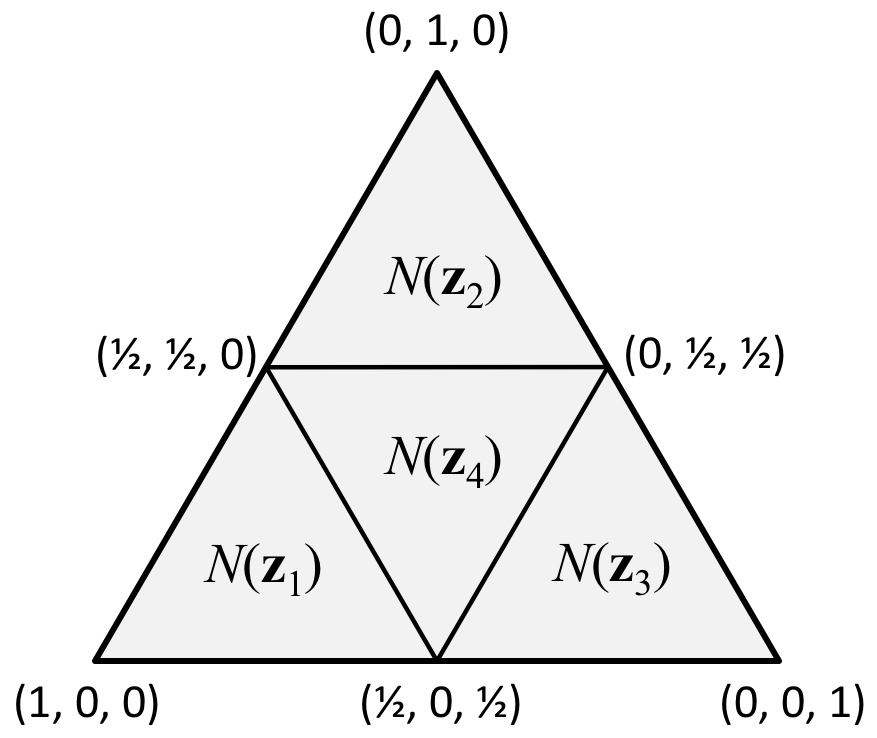
${\mathcal{N}}^{\textup{{CS}}}({\mathbf{z}}_{1})=\{{\mathbf{p}}\in\Delta_{3}:p_{1}\geq{\frac{1}{2}}\}$
${\mathcal{N}}^{\textup{{CS}}}({\mathbf{z}}_{2})=\{{\mathbf{p}}\in\Delta_{3}:p_{2}\geq{\frac{1}{2}}\}$
${\mathcal{N}}^{\textup{{CS}}}({\mathbf{z}}_{3})=\{{\mathbf{p}}\in\Delta_{3}:p_{3}\geq{\frac{1}{2}}\}$
${\mathcal{N}}^{\textup{{CS}}}({\mathbf{z}}_{4})=\{{\mathbf{p}}\in\Delta_{3}:\max(p_{1},p_{2},p_{3})\leq{\frac{1}{2}}\}$

Figure 3: Positive normal sets for the Crammer-Singer surrogate ${\boldsymbol{\psi}}^{\textup{{CS}}}$ for $n=3$, at 4 points ${\mathbf{z}}_{i}={\boldsymbol{\psi}}^{\textup{{CS}}}({\mathbf{u}}_{i})\in{\mathbb{R}}_{+}^{3}$ ($i\in[4]$) for ${\mathbf{u}}_{1}=(1,0,0)^{\top}$, ${\mathbf{u}}_{2}=(0,1,0)^{\top}$, ${\mathbf{u}}_{3}=(0,0,1)^{\top}$, and ${\mathbf{u}}_{4}=(0,0,0)^{\top}$. Calculations of these sets are based on Lemma 9 and can be found in Appendix C.

3 Conditions for Calibration

In this section we give both necessary conditions (Section 3.1) and sufficient conditions (Section 3.2) for a surrogate ${\boldsymbol{\psi}}$ to be calibrated w.r.t. an arbitrary target loss matrix ${\mathbf{L}}$. Both sets of conditions involve the trigger probability sets of ${\mathbf{L}}$ and the positive normal sets of ${\boldsymbol{\psi}}$; in Section 3.3 we give a result that facilitates computation of positive normal sets for certain classes of surrogates ${\boldsymbol{\psi}}$.

3.1 Necessary Conditions for Calibration

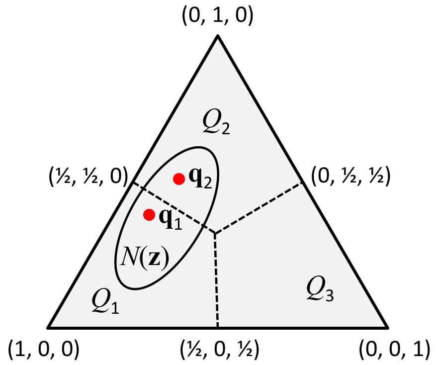
Figure 4: Visual proof of Theorem 6. If a surrogate ${\boldsymbol{\psi}}$ is such that its positive normal set ${\mathcal{N}}^{\psi}({\mathbf{z}})$ at some point ${\mathbf{z}}$ has non-empty intersection with the interiors of two trigger probability sets (say ${\mathcal{Q}}^{\mathbf{L}}_{1}$ and ${\mathcal{Q}}^{\mathbf{L}}_{2}$) of ${\mathbf{L}}$, then ${\boldsymbol{\psi}}$ cannot be ${\mathbf{L}}$-calibrated.

We start by deriving necessary conditions for ${\mathbf{L}}$-calibration of a surrogate loss ${\boldsymbol{\psi}}$. Consider what happens if for some point ${\mathbf{z}}\in{\mathcal{S}}_{\psi}$, the positive normal set of ${\boldsymbol{\psi}}$ at ${\mathbf{z}}$, ${\mathcal{N}}^{\psi}({\mathbf{z}})$, has a non-empty intersection with the interiors of two trigger probability sets of ${\mathbf{L}}$, say ${\mathcal{Q}}^{\mathbf{L}}_{1}$ and ${\mathcal{Q}}^{\mathbf{L}}_{2}$ (see Figure 4 for an illustration), which means $\exists{\mathbf{q}}_{1},{\mathbf{q}}_{2}\in{\mathcal{N}}^{\psi}({\mathbf{z}})$ with $\operatorname{argmin}_{t\in[k]}{\mathbf{q}}_{1}^{\top}{\boldsymbol{\ell}}_{t}=\{1\}$ and $\operatorname{argmin}_{t\in[k]}{\mathbf{q}}_{2}^{\top}{\boldsymbol{\ell}}_{t}=\{2\}$. If ${\boldsymbol{\psi}}$ is ${\mathbf{L}}$-calibrated, then by Lemma 2, we have $\exists\textup{{pred}}^{\prime}:{\mathcal{S}}_{\psi}{\rightarrow}[k]$ such that

$$\inf_{{\mathbf{z}}^{\prime}\in{\mathcal{S}}_{\psi}:\textup{{pred}}^{\prime}({\mathbf{z}}^{\prime})\neq 1}{\mathbf{q}}_{1}^{\top}{\mathbf{z}}^{\prime}~{}=~{}\inf_{{\mathbf{z}}^{\prime}\in{\mathcal{S}}_{\psi}:\textup{{pred}}^{\prime}({\mathbf{z}}^{\prime})\notin\operatorname{argmin}_{t}{\mathbf{q}}_{1}^{\top}{\boldsymbol{\ell}}_{t}}{\mathbf{q}}_{1}^{\top}{\mathbf{z}}^{\prime} > \inf_{{\mathbf{z}}^{\prime}\in{\mathcal{S}}_{\psi}}{\mathbf{q}}_{1}^{\top}{\mathbf{z}}^{\prime}~{}=~{}{\mathbf{q}}_{1}^{\top}{\mathbf{z}}$$

$$\inf_{{\mathbf{z}}^{\prime}\in{\mathcal{S}}_{\psi}:\textup{{pred}}^{\prime}({\mathbf{z}}^{\prime})\neq 2}{\mathbf{q}}_{2}^{\top}{\mathbf{z}}^{\prime}~{}=~{}\inf_{{\mathbf{z}}^{\prime}\in{\mathcal{S}}_{\psi}:\textup{{pred}}^{\prime}({\mathbf{z}}^{\prime})\notin\operatorname{argmin}_{t}{\mathbf{q}}_{2}^{\top}{\boldsymbol{\ell}}_{t}}{\mathbf{q}}_{2}^{\top}{\mathbf{z}}^{\prime} > \inf_{{\mathbf{z}}^{\prime}\in{\mathcal{S}}_{\psi}}{\mathbf{q}}_{2}^{\top}{\mathbf{z}}^{\prime}~{}=~{}{\mathbf{q}}_{2}^{\top}{\mathbf{z}}\,.$$

The first inequality above implies $\textup{{pred}}^{\prime}({\mathbf{z}})=1$; the second inequality implies $\textup{{pred}}^{\prime}({\mathbf{z}})=2$, leading to a contradiction. This gives us the following necessary condition for ${\mathbf{L}}$-calibration of ${\boldsymbol{\psi}}$, which requires the positive normal sets of ${\boldsymbol{\psi}}$ at all points ${\mathbf{z}}\in{\mathcal{S}}_{\psi}$ to be ‘well-behaved’ w.r.t. ${\mathbf{L}}$ in the sense of being contained within individual trigger probability sets of ${\mathbf{L}}$ and generalizes the ‘admissibility’ condition used for 0-1 loss by Tewari and Bartlett (2007):

Theorem 6

Let ${\mathbf{L}}\in{\mathbb{R}}_{+}^{n\times k}$, and let ${\boldsymbol{\psi}}:{\mathcal{C}}{\rightarrow}{\mathbb{R}}_{+}^{n}$ be ${\mathbf{L}}$-calibrated. Then for all points ${\mathbf{z}}\in{\mathcal{S}}_{\psi}$, there exists some $t\in[k]$ such that ${\mathcal{N}}^{\psi}({\mathbf{z}})\subseteq{\mathcal{Q}}^{\mathbf{L}}_{t}$.

Proof  See above discussion.  

In fact, we have the following stronger necessary condition, which requires the positive normal sets of ${\boldsymbol{\psi}}$ not only at all points ${\mathbf{z}}\in{\mathcal{S}}_{\psi}$ but also at all sequences $\{{\mathbf{z}}_{m}\}$ in ${\mathcal{S}}_{\psi}$ to be contained within individual trigger probability sets of ${\mathbf{L}}$:

Theorem 7

Let ${\mathbf{L}}\in{\mathbb{R}}_{+}^{n\times k}$, and let ${\boldsymbol{\psi}}:{\mathcal{C}}{\rightarrow}{\mathbb{R}}_{+}^{n}$ be ${\mathbf{L}}$-calibrated. Then for all sequences $\{{\mathbf{z}}_{m}\}$ in ${\mathcal{S}}_{\psi}$, there exists some $t\in[k]$ such that ${\mathcal{N}}^{\psi}(\{{\mathbf{z}}_{m}\})\subseteq{\mathcal{Q}}^{\mathbf{L}}_{t}$.

Proof  Assume for the sake of contradiction that there is some sequence $\{{\mathbf{z}}_{m}\}$ in ${\mathcal{S}}_{\psi}$ for which ${\mathcal{N}}^{\psi}(\{{\mathbf{z}}_{m}\})$ is not contained in ${\mathcal{Q}}^{\mathbf{L}}_{t}$ for any $t\in[k]$. Then $\forall t\in[k]$, $\exists{\mathbf{q}}_{t}\in{\mathcal{N}}^{\psi}(\{{\mathbf{z}}_{m}\})$ such that ${\mathbf{q}}_{t}\notin{\mathcal{Q}}^{\mathbf{L}}_{t}$, i.e. such that $t\notin\operatorname{argmin}_{t^{\prime}}{\mathbf{q}}_{t}^{\top}{\boldsymbol{\ell}}_{t^{\prime}}$. Now, since ${\boldsymbol{\psi}}$ is ${\mathbf{L}}$-calibrated, by Lemma 25, there exists a function $\textup{{pred}}^{\prime}:{\mathcal{S}}_{\psi}{\rightarrow}[k]$ such that for all ${\mathbf{p}}\in{\mathcal{N}}^{\psi}(\{{\mathbf{z}}_{m}\})$, we have $\textup{{pred}}^{\prime}({\mathbf{z}}_{m})\in\arg\min_{t^{\prime}}{\mathbf{p}}^{\top}{\boldsymbol{\ell}}_{t^{\prime}}$ for all large enough $m$. In particular, for ${\mathbf{p}}={\mathbf{q}}_{t}$, we get $\textup{{pred}}^{\prime}({\mathbf{z}}_{m})\in\operatorname{argmin}_{t^{\prime}}{\mathbf{q}}_{t}^{\top}{\boldsymbol{\ell}}_{t^{\prime}}$ ultimately. Since this is true for each $t\in[k]$, we get $\textup{{pred}}^{\prime}({\mathbf{z}}_{m})\in\cap_{t\in[k]}\operatorname{argmin}_{t^{\prime}}{\mathbf{q}}_{t}^{\top}{\boldsymbol{\ell}}_{t^{\prime}}$ ultimately. However by choice of ${\mathbf{q}}_{t}$, this intersection is empty, thus yielding a contradiction. This completes the proof.  

Note that Theorem 7 includes Theorem 6 as a special case, since ${\mathcal{N}}^{\psi}({\mathbf{z}})={\mathcal{N}}^{\psi}(\{{\mathbf{z}}_{m}\})$ for the constant sequence ${\mathbf{z}}_{m}={\mathbf{z}}~{}\forall m$. We stated Theorem 6 separately above since it had a simple, direct proof that helps build intuition.

Example 6 (Crammer-Singer surrogate is not calibrated for 0-1 loss)

Looking at the positive normal sets of the Crammer-Singer surrogate ${\boldsymbol{\psi}}^{\textup{{CS}}}$ (for $n=3$) shown in Figure 3 and the trigger probability sets of the 0-1 loss ${\mathbf{L}}^{\textup{{0-1}}}$ shown in Figure 2(a), we see that ${\mathcal{N}}^{\textup{{CS}}}({\mathbf{z}}_{4})$ is not contained in any single trigger probability set of ${\mathbf{L}}^{\textup{{0-1}}}$, and therefore applying Theorem 6, it is immediately clear that ${\boldsymbol{\psi}}^{\textup{{CS}}}$ is not ${\mathbf{L}}^{\textup{{0-1}}}$-calibrated (this was also established by Tewari and Bartlett (2007) and Zhang (2004b)).

3.2 Sufficient Condition for Calibration

We now give a sufficient condition for ${\mathbf{L}}$-calibration of a surrogate loss ${\boldsymbol{\psi}}$ that will be helpful in showing calibration of various surrogates. In particular, we show that for a surrogate loss ${\boldsymbol{\psi}}$ to be ${\mathbf{L}}$-calibrated, it is sufficient for the above property of positive normal sets of ${\boldsymbol{\psi}}$ being contained in trigger probability sets of ${\mathbf{L}}$ to hold for only a finite number of points in ${\mathcal{S}}_{\psi}$, as long as the corresponding positive normal sets jointly cover $\Delta_{n}$:

Theorem 8

Let ${\mathbf{L}}\in{\mathbb{R}}_{+}^{n\times k}$ and ${\boldsymbol{\psi}}:{\mathcal{C}}{\rightarrow}{\mathbb{R}}_{+}^{n}$. Suppose there exist $r\in{\mathbb{Z}}_{+}$ and ${\mathbf{z}}_{1},\ldots,{\mathbf{z}}_{r}\in{\mathcal{S}}_{\psi}$ such that $\bigcup_{j=1}^{r}{\mathcal{N}}^{\psi}({\mathbf{z}}_{j})=\Delta_{n}$ and for each $j\in[r]$, $\exists t\in[k]$ such that ${\mathcal{N}}^{\psi}({\mathbf{z}}_{j})\subseteq{\mathcal{Q}}^{\mathbf{L}}_{t}$. Then ${\boldsymbol{\psi}}$ is ${\mathbf{L}}$-calibrated.

Example 7 (Crammer-Singer surrogate is calibrated for ${\mathbf{L}}^{\textup{{(?)}}}$ and ${\mathbf{L}}^{\textup{{ord}}}$ for $n=3$)

Inspecting the positive normal sets of the Crammer-Singer surrogate ${\boldsymbol{\psi}}^{\textup{{CS}}}$ (for $n=3)$ in Figure 3 and the trigger probability sets of the ‘abstain’ loss matrix ${\mathbf{L}}^{\textup{{(?)}}}$ in Figure 2(c), we see that ${\mathcal{N}}^{\textup{{CS}}}({\mathbf{z}}_{i})={\mathcal{Q}}^{\textup{{(?)}}}_{i}~{}\forall i\in[4]$, and therefore by Theorem 8, the Crammer-Singer surrogate ${\boldsymbol{\psi}}^{\textup{{CS}}}$ is ${\mathbf{L}}^{\textup{{(?)}}}$-calibrated. Similarly, looking at the trigger probability sets of the ordinal regression loss matrix ${\mathbf{L}}^{\textup{{ord}}}$ in Figure 2(b) and again applying Theorem 8, we see that the Crammer-Singer surrogate ${\boldsymbol{\psi}}^{\textup{{CS}}}$ is also ${\mathbf{L}}^{\textup{{ord}}}$-calibrated!

Some additional examples of applications of Theorems 6 and 8 are provided in Section 3.3 below. Both the necessary and sufficient conditions above will also be used when we study the convex calibration dimension of a loss matrix ${\mathbf{L}}$ in Section 4.

3.3 Computation of Positive Normal Sets

Both the necessary and sufficient conditions for calibration above involve the positive normal sets ${\mathcal{N}}^{\psi}({\mathbf{z}})$ at various points ${\mathbf{z}}\in{\mathcal{S}}_{\psi}$. Thus in order to use the above results to show that a surrogate ${\boldsymbol{\psi}}$ is (or is not) ${\mathbf{L}}$-calibrated, one needs to be able to compute or characterize the sets ${\mathcal{N}}^{\psi}({\mathbf{z}})$. Here we give a method for computing these sets for certain surrogates ${\boldsymbol{\psi}}$ at certain points ${\mathbf{z}}\in{\mathcal{S}}_{\psi}$. Specifically, the following result gives an explicit method for computing ${\mathcal{N}}^{\psi}({\mathbf{z}})$ for convex surrogate losses ${\boldsymbol{\psi}}$ operating on a convex surrogate space ${\mathcal{C}}\subseteq{\mathbb{R}}^{d}$, at points ${\mathbf{z}}={\boldsymbol{\psi}}({\mathbf{u}})\in{\mathcal{R}}_{\psi}$ for which the subdifferential $\partial\psi_{y}({\mathbf{u}})$ for each $y\in[n]$ can be described as the convex hull of a finite number of points in ${\mathbb{R}}^{d}$; this is particularly applicable for piecewise linear surrogates.^,

Lemma 9

Let ${\mathcal{C}}\subseteq{\mathbb{R}}^{d}$ be a convex set and let ${\boldsymbol{\psi}}:{\mathcal{C}}{\rightarrow}{\mathbb{R}}_{+}^{n}$ be convex. Let ${\mathbf{z}}={\boldsymbol{\psi}}({\mathbf{u}})$ for some ${\mathbf{u}}\in{\mathcal{C}}$ such that $\forall y\in[n]$, the subdifferential of $\psi_{y}$ at ${\mathbf{u}}$ can be written as

$$\partial\psi_{y}({\mathbf{u}})=\operatorname{conv}\big{(}\{{\mathbf{w}}^{y}_{1},\ldots,{\mathbf{w}}^{y}_{s_{y}}\}\big{)}$$

for some $s_{y}\in{\mathbb{Z}}_{+}$ and ${\mathbf{w}}^{y}_{1},\ldots,{\mathbf{w}}^{y}_{s_{y}}\in{\mathbb{R}}^{d}$. Let $s=\sum_{y=1}^{n}s_{y}$, and let

$${\mathbf{A}}=\left[{\mathbf{w}}^{1}_{1}\ldots{\mathbf{w}}^{1}_{s_{1}}{\mathbf{w}}^{2}_{1}\ldots{\mathbf{w}}^{2}_{s_{2}}\ldots\ldots{\mathbf{w}}^{n}_{1}\ldots{\mathbf{w}}^{n}_{s_{n}}\right]\in{\mathbb{R}}^{d\times s}\,;\hskip 21.33955pt{\mathbf{B}}=\left[b_{yj}\right]\in{\mathbb{R}}^{n\times s}\,,$$

where $b_{yj}$ is $1$ if the $j$-th column of ${\mathbf{A}}$ came from $\{{\mathbf{w}}^{y}_{1},\ldots,{\mathbf{w}}^{y}_{s_{y}}\}$ and $0$ otherwise. Then

$${\mathcal{N}}^{\psi}({\mathbf{z}})=\Big{\{}{\mathbf{p}}\in\Delta_{n}:{\mathbf{p}}={\mathbf{B}}{\mathbf{q}}~{}\mbox{for some ${\mathbf{q}}\in\textup{{null}}({\mathbf{A}})\cap\Delta_{s}$}\Big{\}}\,,$$

where $\textup{{null}}({\mathbf{A}})\subseteq{\mathbb{R}}^{s}$ denotes the null space of the matrix ${\mathbf{A}}$.

The proof makes use of the fact that a convex function $\phi:{\mathbb{R}}^{d}{\rightarrow}{\mathbb{R}}$ attains its minimum at ${\mathbf{u}}_{0}\in{\mathbb{R}}^{d}$ iff the subdifferential $\partial\phi({\mathbf{u}}_{0})$ contains ${\mathbf{0}}\in{\mathbb{R}}^{d}$ (e.g. see Bertsekas et al. (2003)). We will also make use of the fact that if $\phi_{1},\phi_{2}:{\mathbb{R}}^{d}{\rightarrow}{\mathbb{R}}$ are convex functions, then the subdifferential of their sum $\phi_{1}+\phi_{2}$ at ${\mathbf{u}}_{0}$ is is equal to the Minkowski sum of the subdifferentials of $\phi_{1}$ and $\phi_{2}$ at ${\mathbf{u}}_{0}$:

$$\partial(\phi_{1}+\phi_{2})({\mathbf{u}}_{0})~{}=~{}\big{\{}{\mathbf{w}}_{1}+{\mathbf{w}}_{2}:{\mathbf{w}}_{1}\in\partial\phi_{1}({\mathbf{u}}_{0}),{\mathbf{w}}_{2}\in\partial\phi_{2}({\mathbf{u}}_{0})\big{\}}\,.$$

Proof  (Proof of Lemma 9)
We have for all ${\mathbf{p}}\in{\mathbb{R}}^{n}$,

$${\mathbf{p}}\in{\mathcal{N}}^{\psi}({\boldsymbol{\psi}}({\mathbf{u}})) \Longleftrightarrow {\mathbf{p}}\in\Delta_{n},~{}{\mathbf{p}}^{\top}{\boldsymbol{\psi}}({\mathbf{u}})\leq{\mathbf{p}}^{\top}{\mathbf{z}}^{\prime}~{}\forall{\mathbf{z}}^{\prime}\in{\mathcal{S}}_{\psi}$$

$$\Longleftrightarrow {\mathbf{p}}\in\Delta_{n},~{}{\mathbf{p}}^{\top}{\boldsymbol{\psi}}({\mathbf{u}})\leq{\mathbf{p}}^{\top}{\mathbf{z}}^{\prime}~{}\forall{\mathbf{z}}^{\prime}\in{\mathcal{R}}_{\psi}$$

$$\Longleftrightarrow {\mathbf{p}}\in\Delta_{n},~{}\mbox{and the convex function $\phi({\mathbf{u}}^{\prime})={\mathbf{p}}^{\top}{\boldsymbol{\psi}}({\mathbf{u}}^{\prime})=\sum_{y=1}^{n}p_{y}\psi_{y}({\mathbf{u}}^{\prime})$}$$

achieves its minimum at $${\mathbf{u}}^{\prime}={\mathbf{u}}$$

$$\Longleftrightarrow {\mathbf{p}}\in\Delta_{n},~{}{\mathbf{0}}\in\sum_{y=1}^{n}p_{y}\partial\psi_{y}({\mathbf{u}})$$

$$\Longleftrightarrow {\mathbf{p}}\in\Delta_{n},~{}{\mathbf{0}}=\sum_{y=1}^{n}p_{y}\sum_{j=1}^{s_{y}}v^{y}_{j}{\mathbf{w}}^{y}_{j}~{}\mbox{for some ${\mathbf{v}}^{y}\in\Delta_{s_{y}}$}$$

$$\Longleftrightarrow {\mathbf{p}}\in\Delta_{n},~{}{\mathbf{0}}=\sum_{y=1}^{n}\sum_{j=1}^{s_{y}}q^{y}_{j}{\mathbf{w}}^{y}_{j}~{}\mbox{for some ${\mathbf{q}}^{y}=p_{y}{\mathbf{v}}^{y}$, ~{} ${\mathbf{v}}^{y}\in\Delta_{s_{y}}$}$$

$$\Longleftrightarrow {\mathbf{p}}\in\Delta_{n},{\mathbf{A}}{\mathbf{q}}={\mathbf{0}}~{}\mbox{for some ${\mathbf{q}}=(p_{1}{\mathbf{v}}^{1},\ldots,p_{n}{\mathbf{v}}^{n})^{\top}\in\Delta_{s}$, ~{} ${\mathbf{v}}^{y}\in\Delta_{s_{y}}$}$$

$$\Longleftrightarrow {\mathbf{p}}={\mathbf{B}}{\mathbf{q}}~{}\mbox{for some ${\mathbf{q}}\in\textup{{null}}({\mathbf{A}})\cap\Delta_{s}$}\,.$$

 

We now give examples of computation of positive normal sets using Lemma 9 for two convex surrogates, both of which operate on the one-dimensional surrogate space ${\mathcal{C}}={\mathbb{R}}$, and as we shall see, turn out to be calibrated w.r.t. the ordinal regression loss ${\mathbf{L}}^{\textup{{ord}}}$ but not w.r.t. the 0-1 loss ${\mathbf{L}}^{\textup{{0-1}}}$ or the ‘abstain’ loss ${\mathbf{L}}^{\textup{{(?)}}}$. As another example of an application of Lemma 9, calculations showing computation of positive normal sets of the Crammer-Singer surrogate (as shown in Figure 3) are given in the appendix.

Example 8 (Positive normal sets of ‘absolute’ surrogate)

Let $n=3$, and let ${\mathcal{C}}={\mathbb{R}}$. Consider the ‘absolute’ surrogate ${\boldsymbol{\psi}}^{\textup{{abs}}}:{\mathbb{R}}{\rightarrow}{\mathbb{R}}_{+}^{3}$ defined as follows:

$$\psi^{\textup{{abs}}}_{y}(u)=|u-y|\qquad\forall y\in[3],\,u\in{\mathbb{R}}\,.$$ (10)

Clearly, ${\boldsymbol{\psi}}^{\textup{{abs}}}$ is a convex function (see Figure 5). Moreover, we have

$${\mathcal{R}}_{\textup{{abs}}}~{}=~{}{\boldsymbol{\psi}}^{\textup{{abs}}}({\mathbb{R}})~{}=~{}\big{\{}(|u-1|,|u-2|,|u-3|)^{\top}:u\in{\mathbb{R}}\big{\}}\subset{\mathbb{R}}_{+}^{3}\,.$$

Now let $u_{1}=1$, $u_{2}=2$, and $u_{3}=3$, and let

$${\mathbf{z}}_{1} = {\boldsymbol{\psi}}^{\textup{{abs}}}(u_{1})~{}=~{}{\boldsymbol{\psi}}^{\textup{{abs}}}(1)~{}=~{}(0,1,2)^{\top}\in{\mathcal{R}}_{\textup{{abs}}}$$

$${\mathbf{z}}_{2} = {\boldsymbol{\psi}}^{\textup{{abs}}}(u_{2})~{}=~{}{\boldsymbol{\psi}}^{\textup{{abs}}}(2)~{}=~{}(1,0,1)^{\top}\in{\mathcal{R}}_{\textup{{abs}}}$$

$${\mathbf{z}}_{3} = {\boldsymbol{\psi}}^{\textup{{abs}}}(u_{3})~{}=~{}{\boldsymbol{\psi}}^{\textup{{abs}}}(3)~{}=~{}(2,1,0)^{\top}\in{\mathcal{R}}_{\textup{{abs}}}\,.$$

Let us consider computing the positive normal sets of ${\boldsymbol{\psi}}^{\textup{{abs}}}$ at the 3 points ${\mathbf{z}}_{1},{\mathbf{z}}_{2},{\mathbf{z}}_{3}$ above. To see that ${\mathbf{z}}_{1}$ satisfies the conditions of Lemma 9, note that

$$\partial\psi^{\textup{{abs}}}_{1}(u_{1})~{}=~{}\partial\psi^{\textup{{abs}}}_{1}(1) = [-1,1]=\operatorname{conv}(\{+1,-1\})\,;$$

$$\partial\psi^{\textup{{abs}}}_{2}(u_{1})~{}=~{}\partial\psi^{\textup{{abs}}}_{2}(1) = \{-1\}=\operatorname{conv}(\{-1\})\,;$$

$$\partial\psi^{\textup{{abs}}}_{3}(u_{1})~{}=~{}\partial\psi^{\textup{{abs}}}_{3}(1) = \{-1\}=\operatorname{conv}(\{-1\})\,.$$

Therefore, we can use Lemma 9 to compute ${\mathcal{N}}^{\textup{{abs}}}({\mathbf{z}}_{1})$. Here $s=4$, and

$${\mathbf{A}}=\left[\begin{array}[]{cccc}+1&-1&-1&-1\end{array}\right]\,;\hskip 14.22636pt{\mathbf{B}}=\left[\begin{array}[]{cccc}1&1&0&0\\ 0&0&1&0\\ 0&0&0&1\end{array}\right]\,.$$

This gives

$${\mathcal{N}}^{\textup{{abs}}}({\mathbf{z}}_{1}) = \big{\{}{\mathbf{p}}\in\Delta_{3}:{\mathbf{p}}=(q_{1}+q_{2},q_{3},q_{4})~{}\mbox{for some ${\mathbf{q}}\in\Delta_{4},~{}q_{1}-q_{2}-q_{3}-q_{4}=0$}\big{\}}$$

$$= \big{\{}{\mathbf{p}}\in\Delta_{3}:{\mathbf{p}}=(q_{1}+q_{2},q_{3},q_{4})~{}\mbox{for some ${\mathbf{q}}\in\Delta_{4},~{}q_{1}=\textstyle{{\frac{1}{2}}}$}\big{\}}$$

$$= \big{\{}{\mathbf{p}}\in\Delta_{3}:p_{1}\geq\textstyle{{\frac{1}{2}}}\big{\}}\,.$$

It is easy to see that ${\mathbf{z}}_{2}$ and ${\mathbf{z}}_{3}$ also satisfy the conditions of Lemma 9; similar computations then yield

$${\mathcal{N}}^{\textup{{abs}}}({\mathbf{z}}_{2}) = \big{\{}{\mathbf{p}}\in\Delta_{3}:p_{1}\leq\textstyle{{\frac{1}{2}}},p_{3}\leq\textstyle{{\frac{1}{2}}}\big{\}}$$

$${\mathcal{N}}^{\textup{{abs}}}({\mathbf{z}}_{3}) = \big{\{}{\mathbf{p}}\in\Delta_{3}:p_{3}\geq\textstyle{{\frac{1}{2}}}\big{\}}\,.$$

The positive normal sets above are shown in Figure 5. Comparing these with the trigger probability sets in Figure 2, we have by Theorem 8 that ${\boldsymbol{\psi}}^{\textup{{abs}}}$ is ${\mathbf{L}}^{\textup{{ord}}}$-calibrated, and by Theorem 6 that ${\boldsymbol{\psi}}^{\textup{{abs}}}$ is not calibrated w.r.t. ${\mathbf{L}}^{\textup{{0-1}}}$ or ${\mathbf{L}}^{\textup{{(?)}}}$.

$\underset{\text{\normalsize{(a)}}}{\includegraphics[width=151.76964pt]{surrogate-abs.pdf}}$           $\underset{\text{\normalsize{(b)}}}{\includegraphics[width=130.08731pt]{pos-normal-abs.png}}$

Figure 5: (a) The ‘absolute’ surrogate ${\boldsymbol{\psi}}^{\textup{{abs}}}:{\mathbb{R}}{\rightarrow}{\mathbb{R}}_{+}^{3}$ (for $n=3$), and (b) its positive normal sets at 3 points ${\mathbf{z}}_{i}={\boldsymbol{\psi}}^{\textup{{abs}}}(u_{i})\in{\mathbb{R}}_{+}^{3}$ ($i\in[3]$) for $u_{1}=1,u_{2}=2,u_{3}=3$. See Example 8 for details.

Example 9 (Positive normal sets of ‘$\epsilon$-insensitive’ surrogate)

Let $n=3$, and let ${\mathcal{C}}={\mathbb{R}}$. Let $\epsilon\in[0,0.5)$, and consider the ‘$\epsilon$-insensitive’ surrogate ${\boldsymbol{\psi}}^{\epsilon}:{\mathbb{R}}{\rightarrow}{\mathbb{R}}_{+}^{3}$ defined as follows:

$$\psi^{\epsilon}_{y}(u)=\big{(}|u-y|-\epsilon\big{)}_{+}\qquad\forall y\in[3],\,u\in{\mathbb{R}}\,.$$ (11)

For $\epsilon=0$, we have ${\boldsymbol{\psi}}^{\epsilon}={\boldsymbol{\psi}}^{\textup{{abs}}}$. Clearly, ${\boldsymbol{\psi}}^{\epsilon}$ is a convex function (see Figure 6). Moreover, we have

$${\mathcal{R}}_{\epsilon}~{}=~{}{\boldsymbol{\psi}}^{\epsilon}({\mathbb{R}})~{}=~{}\big{\{}\big{(}(|u-1|-\epsilon)_{+},(|u-2|-\epsilon)_{+},(|u-3|-\epsilon)_{+}\big{)}^{\top}:u\in{\mathbb{R}}\big{\}}\subset{\mathbb{R}}_{+}^{3}\,.$$

For concreteness, we will take $\epsilon=0.25$ below, but similar computations hold $\forall\epsilon\in(0,0.5)$. Let $u_{1}=1+\epsilon=1.25$, $u_{2}=2-\epsilon=1.75$, $u_{3}=2+\epsilon=2.25$, and $u_{4}=3-\epsilon=2.75$, and let

$${\mathbf{z}}_{1} = {\boldsymbol{\psi}}^{0.25}(u_{1})~{}=~{}{\boldsymbol{\psi}}^{0.25}(1.25)~{}=~{}(0,0.5,1.5)^{\top}\in{\mathcal{R}}_{0.25}$$

$${\mathbf{z}}_{2} = {\boldsymbol{\psi}}^{0.25}(u_{2})~{}=~{}{\boldsymbol{\psi}}^{0.25}(1.75)~{}=~{}(0.5,0,1)^{\top}\in{\mathcal{R}}_{0.25}$$

$${\mathbf{z}}_{3} = {\boldsymbol{\psi}}^{0.25}(u_{3})~{}=~{}{\boldsymbol{\psi}}^{0.25}(2.25)~{}=~{}(1,0,0.5)^{\top}\in{\mathcal{R}}_{0.25}$$

$${\mathbf{z}}_{4} = {\boldsymbol{\psi}}^{0.25}(u_{4})~{}=~{}{\boldsymbol{\psi}}^{0.25}(2.75)~{}=~{}(1.5,0.5,0)^{\top}\in{\mathcal{R}}_{0.25}\,.$$

Let us consider computing the positive normal sets of ${\boldsymbol{\psi}}^{0.25}$ at the 4 points ${\mathbf{z}}_{i}$ ($i\in[4]$) above. To see that ${\mathbf{z}}_{1}$ satisfies the conditions of Lemma 9, note that

$$\partial\psi^{0.25}_{1}(u_{1})~{}=~{}\partial\psi^{0.25}_{1}(1.25) = [0,1]=\operatorname{conv}(\{0,1\})\,;$$

$$\partial\psi^{0.25}_{2}(u_{1})~{}=~{}\partial\psi^{0.25}_{2}(1.25) = \{-1\}=\operatorname{conv}(\{-1\})\,;$$

$$\partial\psi^{0.25}_{3}(u_{1})~{}=~{}\partial\psi^{0.25}_{3}(1.25) = \{-1\}=\operatorname{conv}(\{-1\})\,.$$

Therefore, we can use Lemma 9 to compute ${\mathcal{N}}^{0.25}({\mathbf{z}}_{1})$. Here $s=4$, and

$${\mathbf{A}}=\left[\begin{array}[]{cccc}0&1&-1&-1\end{array}\right]\,;\hskip 14.22636pt{\mathbf{B}}=\left[\begin{array}[]{cccc}1&1&0&0\\ 0&0&1&0\\ 0&0&0&1\end{array}\right]\,.$$

This gives

$${\mathcal{N}}^{0.25}({\mathbf{z}}_{1}) = \big{\{}{\mathbf{p}}\in\Delta_{3}:{\mathbf{p}}=(q_{1}+q_{2},q_{3},q_{4})~{}\mbox{for some ${\mathbf{q}}\in\Delta_{4},~{}q_{2}-q_{3}-q_{4}=0$}\big{\}}$$

$$= \big{\{}{\mathbf{p}}\in\Delta_{3}:{\mathbf{p}}=(q_{1}+q_{2},q_{3},q_{4})~{}\mbox{for some ${\mathbf{q}}\in\Delta_{4},~{}q_{1}+q_{2}\geq q_{3}+q_{4}$}\big{\}}$$

$$= \big{\{}{\mathbf{p}}\in\Delta_{3}:p_{1}\geq\textstyle{{\frac{1}{2}}}\big{\}}\,.$$

Similarly, to see that ${\mathbf{z}}_{2}$ satisfies the conditions of Lemma 9, note that

$$\partial\psi^{0.25}_{1}(u_{2})~{}=~{}\partial\psi^{0.25}_{1}(1.75) = \{1\}=\operatorname{conv}(\{1\})\,;$$

$$\partial\psi^{0.25}_{2}(u_{2})~{}=~{}\partial\psi^{0.25}_{2}(1.75) = [-1,0]=\operatorname{conv}(\{-1,0\})\,;$$

$$\partial\psi^{0.25}_{3}(u_{2})~{}=~{}\partial\psi^{0.25}_{3}(1.75) = \{-1\}=\operatorname{conv}(\{-1\})\,.$$

Again, we can use Lemma 9 to compute ${\mathcal{N}}^{0.25}({\mathbf{z}}_{2})$; here $s=4$, and

$${\mathbf{A}}=\left[\begin{array}[]{cccc}1&-1&0&-1\end{array}\right]\,;\hskip 14.22636pt{\mathbf{B}}=\left[\begin{array}[]{cccc}1&0&0&0\\ 0&1&1&0\\ 0&0&0&1\end{array}\right]\,.$$

This gives

$${\mathcal{N}}^{0.25}({\mathbf{z}}_{2}) = \big{\{}{\mathbf{p}}\in\Delta_{3}:{\mathbf{p}}=(q_{1},q_{2}+q_{3},q_{4})~{}\mbox{for some ${\mathbf{q}}\in\Delta_{4},~{}q_{1}-q_{2}-q_{4}=0$}\big{\}}$$

$$= \big{\{}{\mathbf{p}}\in\Delta_{3}:p_{1}\geq p_{3},~{}p_{1}\leq\textstyle{{\frac{1}{2}}}\big{\}}\,.$$

It is easy to see that ${\mathbf{z}}_{3}$ and ${\mathbf{z}}_{4}$ also satisfy the conditions of Lemma 9; similar computations then yield

$${\mathcal{N}}^{0.25}({\mathbf{z}}_{3}) = \big{\{}{\mathbf{p}}\in\Delta_{3}:p_{1}\leq p_{3},~{}p_{3}\leq\textstyle{{\frac{1}{2}}}\big{\}}$$

$${\mathcal{N}}^{0.25}({\mathbf{z}}_{4}) = \big{\{}{\mathbf{p}}\in\Delta_{3}:p_{3}\geq\textstyle{{\frac{1}{2}}}\big{\}}\,.$$

The positive normal sets above are shown in Figure 6. Comparing these with the trigger probability sets in Figure 2, we have by Theorem 8 that ${\boldsymbol{\psi}}^{0.25}$ is ${\mathbf{L}}^{\textup{{ord}}}$-calibrated, and by Theorem 6 that ${\boldsymbol{\psi}}^{0.25}$ is not calibrated w.r.t. ${\mathbf{L}}^{\textup{{0-1}}}$ or ${\mathbf{L}}^{\textup{{(?)}}}$.

$\underset{\text{\normalsize{(a)}}}{\includegraphics[width=151.76964pt]{surrogate-epsilon.pdf}}$           $\underset{\text{\normalsize{(b)}}}{\includegraphics[width=130.08731pt]{pos-normal-epsilon.png}}$

Figure 6: (a) The ‘$\epsilon$-insensitive’ surrogate ${\boldsymbol{\psi}}^{\epsilon}:{\mathbb{R}}{\rightarrow}{\mathbb{R}}_{+}^{3}$ for $\epsilon=0.25$ (and $n=3$), and (b) its positive normal sets at 4 points ${\mathbf{z}}_{i}={\boldsymbol{\psi}}^{\epsilon}(u_{i})\in{\mathbb{R}}_{+}^{3}$ ($i\in[4]$) for $u_{1}=1.25,u_{2}=1.75,u_{3}=2.25,u_{4}=2.75$. See Example 9 for details.

4 Convex Calibration Dimension

We now turn to the study of a fundamental quantity associated with the property of ${\mathbf{L}}$-calibration. Specifically, in Examples 6 and 7 above, we saw that to develop a surrogate calibrated w.r.t. to the ordinal regression loss ${\mathbf{L}}^{\textup{{ord}}}$ for $n=3$, it was sufficient to consider a surrogate prediction space ${\mathcal{C}}={\mathbb{R}}$, with dimension $d=1$; in addition, the surrogates we considered were convex, and can therefore be used in developing computationally efficient algorithms. In fact the same surrogate prediction space with $d=1$ can be used to develop similar convex surrogate losses calibrated w.r.t. the ${\mathbf{L}}^{\textup{{ord}}}$ for any $n\in{\mathbb{Z}}_{+}$. However not all multiclass loss matrices ${\mathbf{L}}$ have such ‘low-dimensional’ convex surrogates. This raises the natural question of what is the smallest dimension $d$ that supports a convex ${\mathbf{L}}$-calibrated surrogate for a given multiclass loss ${\mathbf{L}}$, and leads us to the following definition:

Definition 10 (Convex calibration dimension)

Let ${\mathbf{L}}\in{\mathbb{R}}_{+}^{n\times k}$. Define the convex calibration dimension (CC dimension) of ${\mathbf{L}}$ as

$$\operatorname{CCdim}({\mathbf{L}}) \stackrel{{\scriptstyle\triangle}}{{=}} \min\big{\{}d\in{\mathbb{Z}}_{+}:\exists~{}\textrm{a convex set ${\mathcal{C}}\subseteq{\mathbb{R}}^{d}$ and a convex surrogate ${\boldsymbol{\psi}}:{\mathcal{C}}{\rightarrow}{\mathbb{R}}_{+}^{n}$}\big{.}$$

$$\big{.}~{}~{}~{}~{}~{}~{}~{}~{}~{}~{}~{}\textrm{that is \ ${\mathbf{L}}$-calibrated}\big{\}}\,,$$

if the above set is non-empty, and $\operatorname{CCdim}({\mathbf{L}})=\infty$ otherwise.

The CC-dimension of a loss matrix ${\mathbf{L}}$ provides an important measure of the ‘complexity’ of designing convex calibrated surrogates for ${\mathbf{L}}$. Indeed, while the computational complexity of minimizing a surrogate loss, as well as that of converting surrogate predictions into target predictions, can depend on factors other than the dimension $d$ of the surrogate space ${\mathcal{C}}\subseteq{\mathbb{R}}^{d}$, in the absence of other guiding factors, one would in general prefer to use a surrogate in a lower dimension $d$ since this involves learning a smaller number of real-valued functions.

From the above discussion, $\operatorname{CCdim}({\mathbf{L}}^{\textup{{ord}}})=1$ for all $n$. In the following, we will be interested in developing an understanding of the CC dimension for general loss matrices ${\mathbf{L}}$, and in particular in deriving upper and lower bounds on this quantity.

4.1 Upper Bounds on the Convex Calibration Dimension

We start with a simple result that establishes that the CC dimension of any multiclass loss matrix ${\mathbf{L}}$ is finite, and in fact is strictly smaller than the number of class labels $n$.

Lemma 11

Let ${\mathbf{L}}\in{\mathbb{R}}_{+}^{n\times k}$. Let ${\mathcal{C}}=\big{\{}{\mathbf{u}}\in{\mathbb{R}}_{+}^{n-1}:\sum_{j=1}^{n-1}u_{j}\leq 1\big{\}}$, and for each $y\in[n]$, let $\psi_{y}:{\mathcal{C}}{\rightarrow}{\mathbb{R}}_{+}$ be given by

$$\psi_{y}({\mathbf{u}})~{}=~{}{\mathbf{1}}(y\neq n)\,(u_{y}-1)^{2}+\sum_{j\in[n-1],j\neq y}u_{j}{}^{2}\,.$$

Then ${\boldsymbol{\psi}}$ is ${\mathbf{L}}$-calibrated. In particular, since ${\boldsymbol{\psi}}$ is convex, $\operatorname{CCdim}({\mathbf{L}})\leq n-1$.

It may appear surprising that the convex surrogate ${\boldsymbol{\psi}}$ in the above lemma, operating on a surrogate space ${\mathcal{C}}\subset{\mathbb{R}}^{n-1}$, is ${\mathbf{L}}$-calibrated for all multiclass losses ${\mathbf{L}}$ on $n$ classes. However this makes intuitive sense, since in principle, for any multiclass problem, if one can estimate the conditional probabilities of the $n$ classes accurately (which requires estimating $n-1$ real-valued functions on ${\mathcal{X}}$), then one can predict a target label that minimizes the expected loss according to these probabilities. Minimizing the above surrogate effectively corresponds to such class probability estimation. Indeed, the above lemma can be shown to hold for any surrogate that is a strictly proper composite multiclass loss (Vernet et al., 2011).

In practice, when the number of class labels $n$ is large (such as in a sequence labeling task, where $n$ is exponential in the length of the input sequence), the above result is not very helpful; in such cases, it is of interest to develop algorithms operating on a surrogate prediction space in a lower-dimensional space. Next we give a different upper bound on the CC dimension that depends on the loss ${\mathbf{L}}$, and for certain losses, can be significantly tighter than the general bound above.

Theorem 12

Let ${\mathbf{L}}\in{\mathbb{R}}_{+}^{n\times k}$. Then $\operatorname{CCdim}({\mathbf{L}})\leq\operatorname{affdim}({\mathbf{L}})$.

Proof  Let $\operatorname{affdim}({\mathbf{L}})=d$. We will construct a convex ${\mathbf{L}}$-calibrated surrogate loss ${\boldsymbol{\psi}}$ with surrogate prediction space ${\mathcal{C}}\subseteq{\mathbb{R}}^{d}$.

Let ${\mathcal{V}}\subseteq{\mathbb{R}}^{n}$ denote the ($d$-dimensional) subspace parallel to the affine hull of the column vectors of ${\mathbf{L}}$, and let ${\mathbf{r}}\in{\mathbb{R}}^{n}$ be the corresponding translation vector, so that ${\mathcal{V}}=\textup{{aff}}(\{{\boldsymbol{\ell}}_{1},\ldots,{\boldsymbol{\ell}}_{k}\})+{\mathbf{r}}$. Let ${\mathbf{v}}_{1},\ldots,{\mathbf{v}}_{d}\in{\mathcal{V}}$ be $d$ linearly independent vectors in ${\mathcal{V}}$. Let $\{{\mathbf{e}}_{1},\ldots,{\mathbf{e}}_{d}\}$ denote the standard basis in ${\mathbb{R}}^{d}$, and define a linear function $\widetilde{{\boldsymbol{\psi}}}:{\mathbb{R}}^{d}{\rightarrow}{\mathbb{R}}^{n}$ by

$$\widetilde{{\boldsymbol{\psi}}}({\mathbf{e}}_{j})={\mathbf{v}}_{j}~{}~{}~{}~{}\forall j\in[d]\,.$$

Then for each ${\mathbf{v}}\in{\mathcal{V}}$, there exists a unique vector ${\mathbf{u}}\in{\mathbb{R}}^{d}$ such that $\widetilde{{\boldsymbol{\psi}}}({\mathbf{u}})={\mathbf{v}}$. In particular, since ${\boldsymbol{\ell}}_{t}+{\mathbf{r}}\in{\mathcal{V}}~{}\forall t\in[k]$, there exist unique vectors ${\mathbf{u}}_{1},\ldots,{\mathbf{u}}_{k}\in{\mathbb{R}}^{d}$ such that for each $t\in[k]$, $\widetilde{{\boldsymbol{\psi}}}({\mathbf{u}}_{t})={\boldsymbol{\ell}}_{t}+{\mathbf{r}}$. Let ${\mathcal{C}}=\operatorname{conv}(\{{\mathbf{u}}_{1},\ldots,{\mathbf{u}}_{k}\})\subseteq{\mathbb{R}}^{d}$, and define ${\boldsymbol{\psi}}:{\mathcal{C}}{\rightarrow}{\mathbb{R}}_{+}^{n}$ as

$${\boldsymbol{\psi}}({\mathbf{u}})=\widetilde{{\boldsymbol{\psi}}}({\mathbf{u}})-{\mathbf{r}}~{}~{}~{}~{}\forall{\mathbf{u}}\in{\mathcal{C}}\,.$$

To see that ${\boldsymbol{\psi}}({\mathbf{u}})\in{\mathbb{R}}_{+}^{n}~{}\forall{\mathbf{u}}\in{\mathcal{C}}$, note that for any ${\mathbf{u}}\in{\mathcal{C}}$, $\exists{\boldsymbol{\alpha}}\in\Delta_{k}$ such that ${\mathbf{u}}=\sum_{t=1}^{k}\alpha_{t}{\mathbf{u}}_{t}$, which gives ${\boldsymbol{\psi}}({\mathbf{u}})=\widetilde{{\boldsymbol{\psi}}}({\mathbf{u}})-{\mathbf{r}}=\big{(}\sum_{t=1}^{k}\alpha_{t}\widetilde{{\boldsymbol{\psi}}}({\mathbf{u}}_{t})\big{)}-{\mathbf{r}}=\big{(}\sum_{t=1}^{k}\alpha_{t}({\boldsymbol{\ell}}_{t}+{\mathbf{r}})\big{)}-{\mathbf{r}}=\sum_{t=1}^{k}\alpha_{t}{\boldsymbol{\ell}}_{t}$ (and ${\boldsymbol{\ell}}_{t}\in{\mathbb{R}}_{+}^{n}~{}\forall t\in[k]$). The function ${\boldsymbol{\psi}}$ is clearly convex. To show ${\boldsymbol{\psi}}$ is ${\mathbf{L}}$-calibrated, we will use Theorem 8. Specifically, consider the $k$ points ${\mathbf{z}}_{t}={\boldsymbol{\psi}}({\mathbf{u}}_{t})={\boldsymbol{\ell}}_{t}\in{\mathcal{R}}_{\psi}$ for $t\in[k]$. By definition of ${\boldsymbol{\psi}}$, we have ${\mathcal{S}}_{\psi}=\operatorname{conv}({\boldsymbol{\psi}}({\mathcal{C}}))=\operatorname{conv}(\{{\boldsymbol{\ell}}_{1},\ldots,{\boldsymbol{\ell}}_{k}\})$; from the definitions of positive normals and trigger probabilities, it then follows that ${\mathcal{N}}^{\psi}({\mathbf{z}}_{t})={\mathcal{N}}^{\psi}({\boldsymbol{\ell}}_{t})={\mathcal{Q}}^{\mathbf{L}}_{t}$ for all $t\in[k]$. Thus by Theorem 8, ${\boldsymbol{\psi}}$ is ${\mathbf{L}}$-calibrated.  

Since $\operatorname{affdim}({\mathbf{L}})$ is equal to either $\operatorname{rank}({\mathbf{L}})$ or $\operatorname{rank}({\mathbf{L}})-1$, this immediately gives us the following corollary:

Corollary 13

Let ${\mathbf{L}}\in{\mathbb{R}}_{+}^{n\times k}$. Then $\operatorname{CCdim}({\mathbf{L}})\leq\operatorname{rank}({\mathbf{L}})$.

Proof  Follows immediately from Theorem 12 and the fact that $\operatorname{affdim}({\mathbf{L}})\leq\operatorname{rank}({\mathbf{L}})$.  

Example 10 (CC dimension of Hamming loss)

Let $n=2^{r}$ for some $r\in{\mathbb{Z}}_{+}$, and consider the Hamming loss ${\mathbf{L}}^{\textup{{Ham}}}\in{\mathbb{R}}_{+}^{n\times n}$ defined in Example 3. As in Example 3, for each $z\in\{0,\ldots,2^{r}-1\}$, let $z_{i}\in\{0,1\}$ denote the $i$-th bit in the $r$-bit binary representation of $z$. For each $y\in[n]$, define ${\boldsymbol{\sigma}}_{y}\in\{\pm 1\}^{r}$ as

$$\sigma_{yi}~{}=~{}2\,(y-1)_{i}-1~{}=~{}\begin{cases}+1&~{}~{}\mbox{if $(y-1)_{i}=1$}\\ -1&~{}~{}\mbox{otherwise.}\end{cases}$$

Then we have

$$\ell^{\textup{{Ham}}}_{yt} = \sum_{i=1}^{r}{\mathbf{1}}\big{(}(y-1)_{i}\neq(t-1)_{i}\big{)}$$

$$= \sum_{i=1}^{r}\bigg{(}\frac{1-\sigma_{yi}\sigma_{ti}}{2}\bigg{)}$$

$$= \frac{r}{2}-\sum_{i=1}^{r}\frac{\sigma_{yi}\sigma_{ti}}{2}~{}~{}~{}~{}\forall y,t\in[n]\,.$$

Thus $\operatorname{affdim}({\mathbf{L}}^{\textup{{Ham}}})\leq r$, and therefore by Theorem 12, we have $\operatorname{CCdim}({\mathbf{L}}^{\textup{{Ham}}})\leq r$. This is a significantly tighter upper bound than the bound of $2^{r}-1$ given by Lemma 11.

4.2 Lower Bound on the Convex Calibration Dimension

In this section we give a lower bound on the CC dimension of a loss matrix ${\mathbf{L}}$ and illustrate it by using it to calculate the CC dimension of the 0-1 loss. In Section 5 we will explore applications of the lower bound to obtaining impossibility results on the existence of convex calibrated surrogates in low-dimensional surrogate spaces for certain types of subset ranking losses. We will need the following definition:

Definition 14 (Feasible subspace dimension)

The feasible subspace dimension of a convex set ${\mathcal{Q}}\subseteq{\mathbb{R}}^{n}$ at a point ${\mathbf{p}}\in{\mathcal{Q}}$, denoted by $\mu_{\mathcal{Q}}({\mathbf{p}})$, is defined as the dimension of the subspace ${\mathcal{F}}_{\mathcal{Q}}({\mathbf{p}})\cap(-{\mathcal{F}}_{\mathcal{Q}}({\mathbf{p}}))$, where ${\mathcal{F}}_{\mathcal{Q}}({\mathbf{p}})$ is the cone of feasible directions of ${\mathcal{Q}}$ at ${\mathbf{p}}$.

In essence, the feasible subspace dimension of a convex set $Q$ at a point ${\mathbf{p}}\in{\mathcal{Q}}$ is simply the dimension of the smallest face of ${\mathcal{Q}}$ containing ${\mathbf{p}}$; see Figure 7 for an illustration.

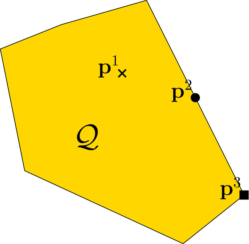
(a) Convex set ${\mathcal{Q}}$

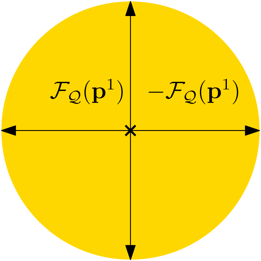
(b) $\operatorname{dim}({\mathcal{F}}_{\mathcal{Q}}({\mathbf{p}}^{1})\cap(-{\mathcal{F}}_{\mathcal{Q}}({\mathbf{p}}^{1})))=2$

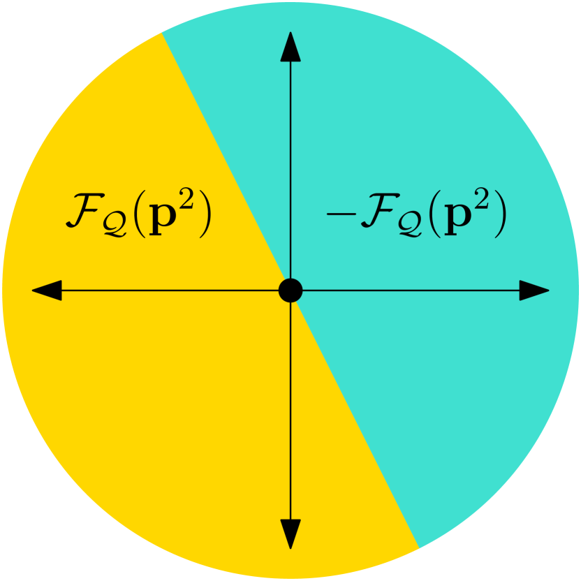
(c) $\operatorname{dim}({\mathcal{F}}_{\mathcal{Q}}({\mathbf{p}}^{2})\cap(-{\mathcal{F}}_{\mathcal{Q}}({\mathbf{p}}^{2})))=1$

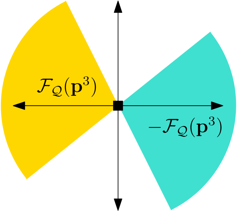
(d) $\operatorname{dim}({\mathcal{F}}_{\mathcal{Q}}({\mathbf{p}}^{3})\cap(-{\mathcal{F}}_{\mathcal{Q}}({\mathbf{p}}^{3})))=0$

Figure 7: Illustration of feasible subspace dimension $\mu_{\mathcal{Q}}({\mathbf{p}})$ of a 2-dimensional convex set ${\mathcal{Q}}$ at three points ${\mathbf{p}}={\mathbf{p}}^{1},{\mathbf{p}}^{2},{\mathbf{p}}^{3}$. Here $\mu_{\mathcal{Q}}({\mathbf{p}}^{1})=2$, $\mu_{\mathcal{Q}}({\mathbf{p}}^{2})=1$, and $\mu_{\mathcal{Q}}({\mathbf{p}}^{3})=0$.

Both the proof of the lower bound we will provide below and its applications make use of the following lemma, which gives a method to calculate the feasible subspace dimension for certain convex sets ${\mathcal{Q}}$ and points ${\mathbf{p}}\in{\mathcal{Q}}$:

Lemma 15

Let ${\mathcal{Q}}=\big{\{}{\mathbf{q}}\in{\mathbb{R}}^{n}:{\mathbf{A}}^{1}{\mathbf{q}}\leq{\mathbf{b}}^{1},{\mathbf{A}}^{2}{\mathbf{q}}\leq{\mathbf{b}}^{2},{\mathbf{A}}^{3}{\mathbf{q}}={\mathbf{b}}^{3}\big{\}}$. Let ${\mathbf{p}}\in{\mathcal{Q}}$ be such that ${\mathbf{A}}^{1}{\mathbf{p}}={\mathbf{b}}^{1}$, ${\mathbf{A}}^{2}{\mathbf{p}}<{\mathbf{b}}^{2}$. Then $\mu_{\mathcal{Q}}({\mathbf{p}})=\operatorname{nullity}\Big{(}\Big{[}\begin{matrix}{\mathbf{A}}^{1}\\ {\mathbf{A}}^{3}\end{matrix}\Big{]}\Big{)}$.

Proof  We will show that ${\mathcal{F}}_{\mathcal{Q}}({\mathbf{p}})\cap(-{\mathcal{F}}_{\mathcal{Q}}({\mathbf{p}}))=\textup{{null}}\Big{(}\Big{[}\begin{matrix}{\mathbf{A}}^{1}\\ {\mathbf{A}}^{3}\end{matrix}\Big{]}\Big{)}$, from which the lemma follows.
First, let ${\mathbf{v}}\in\textup{{null}}\Big{(}\Big{[}\begin{matrix}{\mathbf{A}}^{1}\\ {\mathbf{A}}^{3}\end{matrix}\Big{]}\Big{)}$. Then for $\epsilon>0$, we have

$${\mathbf{A}}^{1}({\mathbf{p}}+\epsilon{\mathbf{v}}) = {\mathbf{A}}^{1}{\mathbf{p}}+\epsilon{\mathbf{A}}^{1}{\mathbf{v}}~{}=~{}{\mathbf{A}}^{1}{\mathbf{p}}+{\mathbf{0}}~{}=~{}{\mathbf{b}}^{1}$$

$${\mathbf{A}}^{2}({\mathbf{p}}+\epsilon{\mathbf{v}}) < {\mathbf{b}}^{2}~{}~{}~{}\text{for small enough $\epsilon$, since ${\mathbf{A}}^{2}{\mathbf{p}}<{\mathbf{b}}^{2}$}$$

$${\mathbf{A}}^{3}({\mathbf{p}}+\epsilon{\mathbf{v}}) = {\mathbf{A}}^{3}{\mathbf{p}}+\epsilon{\mathbf{A}}^{3}{\mathbf{v}}~{}=~{}{\mathbf{A}}^{3}{\mathbf{p}}+{\mathbf{0}}~{}=~{}{\mathbf{b}}^{3}\,.$$

Thus ${\mathbf{v}}\in{\mathcal{F}}_{\mathcal{Q}}({\mathbf{p}})$. Similarly, we can show $-{\mathbf{v}}\in{\mathcal{F}}_{\mathcal{Q}}({\mathbf{p}})$. Thus ${\mathbf{v}}\in{\mathcal{F}}_{\mathcal{Q}}({\mathbf{p}})\cap(-{\mathcal{F}}_{\mathcal{Q}}({\mathbf{p}}))$, giving $\textup{{null}}\Big{(}\Big{[}\begin{matrix}{\mathbf{A}}^{1}\\ {\mathbf{A}}^{3}\end{matrix}\Big{]}\Big{)}\subseteq{\mathcal{F}}_{\mathcal{Q}}({\mathbf{p}})\cap(-{\mathcal{F}}_{\mathcal{Q}}({\mathbf{p}}))$. Now let ${\mathbf{v}}\in{\mathcal{F}}_{\mathcal{Q}}({\mathbf{p}})\cap(-{\mathcal{F}}_{\mathcal{Q}}({\mathbf{p}}))$. Then for small enough $\epsilon>0$, we have both ${\mathbf{A}}^{1}({\mathbf{p}}+\epsilon{\mathbf{v}})\leq{\mathbf{b}}^{1}$ and ${\mathbf{A}}^{1}({\mathbf{p}}-\epsilon{\mathbf{v}})\leq{\mathbf{b}}^{1}$. Since ${\mathbf{A}}^{1}{\mathbf{p}}={\mathbf{b}}^{1}$, this gives ${\mathbf{A}}^{1}{\mathbf{v}}={\mathbf{0}}$. Similarly, for small enough $\epsilon>0$, we have ${\mathbf{A}}^{3}({\mathbf{p}}+\epsilon{\mathbf{v}})={\mathbf{b}}^{3}$; since ${\mathbf{A}}^{3}{\mathbf{p}}={\mathbf{b}}^{3}$, this gives ${\mathbf{A}}^{3}{\mathbf{v}}={\mathbf{0}}$. Thus $\Big{[}\begin{matrix}{\mathbf{A}}^{1}\\ {\mathbf{A}}^{3}\end{matrix}\Big{]}{\mathbf{v}}={\mathbf{0}}$, giving ${\mathcal{F}}_{\mathcal{Q}}({\mathbf{p}})\cap(-{\mathcal{F}}_{\mathcal{Q}}({\mathbf{p}}))\subseteq\textup{{null}}\Big{(}\Big{[}\begin{matrix}{\mathbf{A}}^{1}\\ {\mathbf{A}}^{3}\end{matrix}\Big{]}\Big{)}$.  

The following gives a lower bound on the CC dimension of a loss matrix ${\mathbf{L}}$ in terms of the feasible subspace dimension of the trigger probability sets ${\mathcal{Q}}^{{\mathbf{L}}}_{t}$ at points ${\mathbf{p}}\in{\mathcal{Q}}^{\mathbf{L}}_{t}$:

Theorem 16

Let ${\mathbf{L}}\in{\mathbb{R}}_{+}^{n\times k}$. Let ${\mathbf{p}}\in\Delta_{n}$ and $t\in\arg\min_{t^{\prime}}{\mathbf{p}}^{\top}{\boldsymbol{\ell}}_{t^{\prime}}$ (equivalently, let ${\mathbf{p}}\in{\mathcal{Q}}^{\mathbf{L}}_{t}$). Then

$$\operatorname{CCdim}({\mathbf{L}})\geq\|{\mathbf{p}}\|_{0}-\mu_{{\mathcal{Q}}^{{\mathbf{L}}}_{t}}({\mathbf{p}})-1\,.$$

The above lower bound allows us to calculate precisely the CC dimension of the 0-1 loss:

Example 11 (CC dimension of 0-1 loss)

Let $n\in{\mathbb{Z}}_{+}$, and consider the 0-1 loss ${\mathbf{L}}^{\textup{{0-1}}}\in{\mathbb{R}}_{+}^{n\times n}$ defined in Example 1. Take ${\mathbf{p}}=(\frac{1}{n},\ldots,\frac{1}{n})^{\top}\in\Delta_{n}$. Then ${\mathbf{p}}\in{\mathcal{Q}}^{\textup{{0-1}}}_{t}$ for all $t\in[k]=[n]$ (see Figure 2); in particular, we have ${\mathbf{p}}\in{\mathcal{Q}}^{\textup{{0-1}}}_{1}$. Now ${\mathcal{Q}}^{\textup{{0-1}}}_{1}$ can be written as

$${\mathcal{Q}}^{\textup{{0-1}}}_{1} = \big{\{}{\mathbf{q}}\in\Delta_{n}:q_{1}\geq q_{y}~{}\forall y\in\{2,\ldots,n\}\big{\}}$$

$$= \big{\{}{\mathbf{q}}\in{\mathbb{R}}^{n}:\big{[}{-{\mathbf{e}}_{n-1}}\,\,\,{\mathbf{I}}_{n-1}\big{]}{\mathbf{q}}\leq{\mathbf{0}},-{\mathbf{q}}\leq{\mathbf{0}},{\mathbf{e}}_{n}^{\top}{\mathbf{q}}=1\}\,,$$

where ${\mathbf{e}}_{n-1}$, ${\mathbf{e}}_{n}$ denote the $(n-1)\times 1$ and $n\times 1$ all ones vectors, respectively, and ${\mathbf{I}}_{n-1}$ denotes the $(n-1)\times(n-1)$ identity matrix. Moreover, we have $\big{[}{-{\mathbf{e}}_{n-1}}\,\,\,{\mathbf{I}}_{n-1}\big{]}{\mathbf{p}}=0$, $-{\mathbf{p}}<{\mathbf{0}}$. Therefore, by Lemma 15, we have

$$\mu_{{\mathcal{Q}}^{\textup{{0-1}}}_{1}}({\mathbf{p}})=\operatorname{nullity}\left(\left[\begin{matrix}{-{\mathbf{e}}_{n-1}}\,\,\,{\mathbf{I}}_{n-1}\\[2.0pt] {\mathbf{e}}_{n}^{\top}\end{matrix}\right]\right)=\operatorname{nullity}\left(\left[\begin{matrix}-1\,\,1\,\,0\,\,\ldots\,\,0\\ -1\,\,0\,\,1\,\,\ldots\,\,0\\ \vdots\\ -1\,\,0\,\,0\,\,\ldots\,\,1\\ ~{}~{}~{}1\,\,1\,\,1\,\,\ldots\,\,1\end{matrix}\right]\right)=0\,.$$

Moreover, $\|{\mathbf{p}}\|_{0}=n$. Thus by Theorem 16, we have $\operatorname{CCdim}({\mathbf{L}}^{\textup{{0-1}}})\geq n-1$. Combined with the upper bound of Lemma 11, this gives $\operatorname{CCdim}({\mathbf{L}}^{\textup{{0-1}}})=n-1$.

4.3 Tightness of Bounds

The upper and lower bounds above are not necessarily tight in general. For example, for the $n$-class ordinal regression loss of Example 2, we know that $\operatorname{CCdim}({\mathbf{L}}^{\textup{{ord}}})=1$; however the upper bound of Theorem 12 only gives $\operatorname{CCdim}({\mathbf{L}}^{\textup{{ord}}})\leq n-1$. Similarly, for the $n$-class abstain loss of Example 4, it can be shown that $\operatorname{CCdim}({\mathbf{L}}^{\textup{{(?)}}})=O(\ln n)$ (in fact we conjecture it to be $\Theta(\ln n)$) (Ramaswamy et al., 2015), whereas the upper bound of Theorem 12 gives $\operatorname{CCdim}({\mathbf{L}}^{\textup{{(?)}}})\leq n$, and the lower bound of Theorem 16 yields only $\operatorname{CCdim}({\mathbf{L}}^{\textup{{(?)}}})\geq 1$. However, as we show below, for certain losses ${\mathbf{L}}$, the bounds of Theorems 12 and 16 are in fact tight (upto an additive constant of $1$).

Lemma 17

Let ${\mathbf{L}}\in{\mathbb{R}}_{+}^{n\times k}$. Let ${\mathbf{p}}\in\operatorname{relint}(\Delta_{n})$ and $c\in{\mathbb{R}}_{+}$ be such that ${\mathbf{p}}^{\top}{\boldsymbol{\ell}}_{t}=c~{}\forall t\in[k]$. Then $\forall t\in[k]$,

$$\mu_{{\mathcal{Q}}^{\mathbf{L}}_{t}}({\mathbf{p}})\leq n-\operatorname{affdim}({\mathbf{L}})\,.$$

Proof  Since ${\mathbf{p}}^{\top}{\boldsymbol{\ell}}_{t}=c~{}\forall t\in[k]$, we have ${\mathbf{p}}\in{\mathcal{Q}}^{\mathbf{L}}_{t}~{}\forall t\in[k]$. In particular, we have ${\mathbf{p}}\in{\mathcal{Q}}^{\mathbf{L}}_{1}$. Now

$${\mathcal{Q}}^{\mathbf{L}}_{1}~{}=~{}\left\{{\mathbf{q}}\in{\mathbb{R}}^{n}:\left[\begin{matrix}({\boldsymbol{\ell}}_{2}-{\boldsymbol{\ell}}_{1})^{\top}\\ \vdots\\ ({\boldsymbol{\ell}}_{k}-{\boldsymbol{\ell}}_{1})^{\top}\end{matrix}\right]{\mathbf{q}}\geq{\mathbf{0}},-{\mathbf{q}}\leq{\mathbf{0}},{\mathbf{e}}_{n}^{\top}{\mathbf{q}}=1\right\}\,.$$

Moreover, $\left[\begin{matrix}({\boldsymbol{\ell}}_{2}-{\boldsymbol{\ell}}_{1})^{\top}\\ \vdots\\ ({\boldsymbol{\ell}}_{k}-{\boldsymbol{\ell}}_{1})^{\top}\end{matrix}\right]{\mathbf{p}}={\mathbf{0}}$ and $-{\mathbf{p}}<{\mathbf{0}}$. Therefore, by Lemma 15, we have

$$\mu_{{\mathcal{Q}}^{\mathbf{L}}_{1}}({\mathbf{p}})~{}=~{}\operatorname{nullity}\left(\left[\begin{matrix}({\boldsymbol{\ell}}_{2}-{\boldsymbol{\ell}}_{1})^{\top}\\ \vdots\\ ({\boldsymbol{\ell}}_{k}-{\boldsymbol{\ell}}_{1})^{\top}\\ {\mathbf{e}}_{n}^{\top}\end{matrix}\right]\right)~{}=~{}n-\operatorname{rank}\left(\left[\begin{matrix}({\boldsymbol{\ell}}_{2}-{\boldsymbol{\ell}}_{1})^{\top}\\ \vdots\\ ({\boldsymbol{\ell}}_{k}-{\boldsymbol{\ell}}_{1})^{\top}\\ {\mathbf{e}}_{n}^{\top}\end{matrix}\right]\right)~{}\leq~{}n-\operatorname{affdim}({\mathbf{L}})\,.$$

A similar proof holds for $\mu_{{\mathcal{Q}}^{\mathbf{L}}_{t}}({\mathbf{p}})$ for all other $t\in[k]$.  

Combining the above result with Theorem 16 immediately gives the following:

Theorem 18

Let ${\mathbf{L}}\in{\mathbb{R}}_{+}^{n\times k}$. If $\exists{\mathbf{p}}\in\operatorname{relint}(\Delta_{n}),c\in{\mathbb{R}}_{+}$ such that ${\mathbf{p}}^{\top}{\boldsymbol{\ell}}_{t}=c~{}\forall t\in[k]$, then

$$\operatorname{CCdim}({\mathbf{L}})\geq\operatorname{affdim}({\mathbf{L}})-1\,.$$

Proof  Follows immediately from Theorem 16 and Lemma 17.  

Intuitively, the condition that $\exists{\mathbf{p}}\in\operatorname{relint}(\Delta_{n}),c\in{\mathbb{R}}_{+}$ such that ${\mathbf{p}}^{\top}{\boldsymbol{\ell}}_{t}=c~{}\forall t\in[k]$ in Lemma 17 and Theorem 18 above captures the essence of a hard problem: in this case, if the underlying label probability distribution ${\mathbf{p}}^{\prime}$ is very close to ${\mathbf{p}}$, then it becomes hard to decide which element $t\in[k]$ is an optimal prediction. This is essentially what leads the lower bound on the CC-dimension to become tight in this case.

A particularly useful application of Theorem 18 is to losses ${\mathbf{L}}$ whose columns ${\boldsymbol{\ell}}_{t}$ can be obtained from one another by permuting entries:

Corollary 19

Let ${\mathbf{L}}\in{\mathbb{R}}_{+}^{n\times k}$ be such that all columns of ${\mathbf{L}}$ can be obtained from one another by permuting entries, i.e. $\forall t_{1},t_{2}\in[k],~{}\exists\sigma\in\Pi_{n}$ such that $\ell_{y,t_{2}}=\ell_{\sigma(y),t_{1}}~{}\forall y\in[n]$. Then

$$\operatorname{CCdim}({\mathbf{L}})\geq\operatorname{affdim}({\mathbf{L}})-1\,.$$

Proof  Let ${\mathbf{p}}=\big{(}\frac{1}{n},\ldots,\frac{1}{n}\big{)}^{\top}\in\operatorname{relint}(\Delta_{n})$. Let $c=\frac{\|{\boldsymbol{\ell}}_{1}\|_{1}}{n}$. Then under the given condition, ${\mathbf{p}}^{\top}{\boldsymbol{\ell}}_{t}=c~{}\forall t\in[k]$. The result then follows from Theorem 18.  

We will use the above corollary in establishing lower bounds on the CC dimension of certain subset ranking losses below.

5 Applications to Subset Ranking

We now consider applications of the above framework to analyzing various subset ranking problems, where each instance $x\in{\mathcal{X}}$ consists of a query together with a set of $r$ documents (for simplicity, $r\in{\mathbb{Z}}_{+}$ here is fixed), and the goal is to learn a prediction model which given such an instance predicts a ranking (permutation) of the $r$ documents (Cossock and Zhang, 2008). We consider three popular losses used for subset ranking: the normalized discounted cumulative gain (NDCG) loss, the pairwise disagreement (PD) loss, and the mean average precision (MAP) loss. Each of these subset ranking losses can be viewed as a specific type of multiclass loss acting on a certain label space ${\mathcal{Y}}$ and prediction space $\widehat{{\mathcal{Y}}}$. In particular, for the NDCG loss, the label space ${\mathcal{Y}}$ contains $r$-dimensional multi-valued relevance vectors; for PD loss, ${\mathcal{Y}}$ contains directed acyclic graphs on $r$ nodes; and for MAP loss, ${\mathcal{Y}}$ contains $r$-dimensional binary relevance vectors. In each case, the prediction space $\widehat{{\mathcal{Y}}}$ is the set of permutations of $r$ objects: $\widehat{{\mathcal{Y}}}=\Pi_{r}$. We study the convex calibration dimension of these losses below. Specifically, we show that the CC dimension of the NDCG loss is upper bounded by $r$ (Section 5.1), and that of both the PD and MAP losses is lower bounded by a quadratic function of $r$ (Sections 5.2 and 5.3). Our result on the CC dimension of the NDCG loss is consistent with previous results in the literature showing the existence of $r$-dimensional convex calibrated surrogates for NDCG (Ravikumar et al., 2011; Buffoni et al., 2011); our results on the CC dimension of the PD and MAP losses strengthen previous results of Calauzènes et al. (2012), who showed non-existence of $r$-dimensional convex calibrated surrogates (with a fixed argsort predictor) for PD and MAP.

5.1 Normalized Discounted Cumulative Gain (NDCG)

The NDCG loss is widely used in information retrieval applications (Järvelin and Kekäläinen, 2000). Here ${\mathcal{Y}}$ is the set of $r$-dimensional relevance vectors with say $s$ relevance levels, ${\mathcal{Y}}=\{0,1,\ldots,s-1\}^{r}$, and $\widehat{{\mathcal{Y}}}$ is the set of permutations of $r$ objects, $\widehat{{\mathcal{Y}}}=\Pi_{r}$ (thus here $n=|{\mathcal{Y}}|=s^{r}$ and $k=|\widehat{{\mathcal{Y}}}|=r!$). The loss on predicting a permutation $\sigma\in\Pi_{r}$ when the true label is ${\mathbf{y}}\in\{0,1,\ldots,s-1\}^{r}$ is given by

$$\ell^{\textup{{NDCG}}}({\mathbf{y}},\sigma)~{}=~{}1-\frac{1}{z({\mathbf{y}})}\sum_{i=1}^{r}\frac{2^{y_{i}}-1}{\log_{2}(\sigma(i)+1)}\,,$$

where $z({\mathbf{y}})$ is a normalizer that ensures the loss is non-negative and depends only on ${\mathbf{y}}$. The NDCG loss can therefore be viewed as a multiclass loss matrix ${\mathbf{L}}^{\textup{{NDCG}}}\in{\mathbb{R}}_{+}^{s^{r}\times r!}$. Clearly, $\operatorname{affdim}({\mathbf{L}}^{\textup{{NDCG}}})\leq r$, and therefore by Theorem 12, we have

$$\operatorname{CCdim}({\mathbf{L}}^{\textup{{NDCG}}})~{}\leq~{}r\,.$$

Indeed, previous results in the literature have shown the existence of $r$-dimensional convex calibrated surrogates for NDCG (Ravikumar et al., 2011; Buffoni et al., 2011).

5.2 Pairwise Disagreement (PD)

Here the label space ${\mathcal{Y}}$ is the set of all directed acyclic graphs (DAGs) on $r$ vertices, which we shall denote as ${\mathcal{G}}_{r}$; for each directed edge $(i,j)$ in a graph $G\in{\mathcal{G}}_{r}$ associated with an instance $x\in{\mathcal{X}}$, the $i$-th document in the document set in $x$ is preferred over the $j$-th document. The prediction space $\widehat{{\mathcal{Y}}}$ is again the set of permutations of $r$ objects, $\widehat{{\mathcal{Y}}}=\Pi_{r}$. The loss on predicting a permutation $\sigma\in\Pi_{r}$ when the true label is $G\in{\mathcal{G}}_{r}$ is given by

$$\ell^{\textup{{PD}}}(G,\sigma) = \sum_{(i,j)\in G}{\mathbf{1}}\big{(}\sigma(i)>\sigma(j)\big{)}$$

$$= \sum_{i=1}^{r}\sum_{j=1}^{r}{\mathbf{1}}\big{(}(i,j)\in G\big{)}\cdot{\mathbf{1}}\big{(}\sigma(i)>\sigma(j)\big{)}$$

$$= \sum_{i=1}^{r}\sum_{j=1}^{i-1}{\mathbf{1}}\big{(}(i,j)\in G\big{)}\cdot{\mathbf{1}}\big{(}\sigma(i)>\sigma(j)\big{)}+{\mathbf{1}}\big{(}(j,i)\in G\big{)}\cdot\Big{(}1-{\mathbf{1}}\big{(}\sigma(i)>\sigma(j)\big{)}\Big{)}$$

$$= \sum_{i=1}^{r}\sum_{j=1}^{i-1}\Big{(}{\mathbf{1}}\big{(}(i,j)\in G\big{)}-{\mathbf{1}}\big{(}(j,i)\in G\big{)}\Big{)}\cdot{\mathbf{1}}\big{(}\sigma(i)>\sigma(j)\big{)}+\sum_{i=1}^{r}\sum_{j=1}^{i-1}{\mathbf{1}}\big{(}(j,i)\in G\big{)}\,.$$

The PD loss can be viewed as a multiclass loss matrix ${\mathbf{L}}^{\textup{{PD}}}\in{\mathbb{R}}_{+}^{|{\mathcal{G}}_{r}|\times r!}$. Note that the second term in the sum above depends only the label $G$; removing this term amounts to simply subtracting a fixed vector from each column of the loss matrix, which does not change the properties of the minimizer of the loss or its CC dimension. We can therefore consider the following loss instead:

$$\widetilde{\ell}^{\textup{{PD}}}(G,\sigma)~{}=~{}\sum_{i=1}^{r}\sum_{j=1}^{i-1}\Big{(}{\mathbf{1}}\big{(}(i,j)\in G\big{)}-{\mathbf{1}}\big{(}(j,i)\in G\big{)}\Big{)}\cdot{\mathbf{1}}\big{(}\sigma(i)>\sigma(j)\big{)}\,.$$

The resulting loss matrix $\widetilde{{\mathbf{L}}}^{\textup{{PD}}}$ clearly has rank at most $\frac{r(r-1)}{2}$. Therefore, by Corollary 13, we have

$$\operatorname{CCdim}({\mathbf{L}}^{\textup{{PD}}})~{}=~{}\operatorname{CCdim}(\widetilde{{\mathbf{L}}}^{\textup{{PD}}})~{}\leq~{}\frac{r(r-1)}{2}\,.$$

In fact one can show that the rank of $\widetilde{{\mathbf{L}}}^{\textup{{PD}}}$ is exactly $\frac{r(r-1)}{2}$:

Proposition 20

$\operatorname{rank}(\widetilde{{\mathbf{L}}}^{\textup{{PD}}})=\frac{r(r-1)}{2}$.

Moreover, it is easy to see that the columns of $\widetilde{{\mathbf{L}}}^{\textup{{PD}}}$ can all be obtained from one another by permuting entries. Therefore, by Corollary 19, we also have

$$\operatorname{CCdim}({\mathbf{L}}^{\textup{{PD}}})~{}=~{}\operatorname{CCdim}(\widetilde{{\mathbf{L}}}^{\textup{{PD}}})~{}\geq~{}\frac{r(r-1)}{2}-2\,.$$

Informally, this implies that a convex surrogate that achieves calibration w.r.t. ${\mathbf{L}}^{\textup{{PD}}}$ over the full probability simplex must effectively ‘estimate’ all edge weights. Formally, this strengthens previous results of Duchi et al. (2010) and Calauzènes et al. (2012). In particular, Duchi et al. (2010) showed that certain popular $r$-dimensional convex surrogates are not calibrated for the PD loss, and conjectured that such convex calibrated surrogates (in $r$ dimensions) do not exist; Calauzènes et al. (2012) showed that indeed there do not exist any $r$-dimensional convex surrogates that use argsort as the predictor and are calibrated for the PD loss. The above result allows us to go further and conclude that in fact, one cannot design convex calibrated surrogates for the PD loss in any prediction space of less than $\frac{r(r-1)}{2}-2$ dimensions (regardless of the predictor used).

5.3 Mean Average Precision (MAP)

Here the label space ${\mathcal{Y}}$ is the set of all (non-zero) $r$-dimensional binary relevance vectors, ${\mathcal{Y}}=\{0,1\}^{r}\setminus\{{\mathbf{0}}\}$, and the prediction space $\widehat{{\mathcal{Y}}}$ is again the set of permutations of $r$ objects, $\widehat{{\mathcal{Y}}}=\Pi_{r}$. The loss on predicting a permutation $\sigma\in\Pi_{r}$ when the true label is ${\mathbf{y}}\in\{0,1\}^{r}\setminus\{{\mathbf{0}}\}$ is given by

$$\ell^{\textup{{MAP}}}({\mathbf{y}},\sigma) = 1-\frac{1}{\|{\mathbf{y}}\|_{1}}\sum_{i:y_{i}=1}\frac{1}{\sigma(i)}\sum_{j=1}^{\sigma(i)}y_{\sigma^{-1}(j)}$$ (12)

$$= 1-\frac{1}{\|{\mathbf{y}}\|_{1}}\sum_{i=1}^{r}\frac{y_{i}}{\sigma(i)}\sum_{j=1}^{\sigma(i)}y_{\sigma^{-1}(j)}$$

$$= 1-\frac{1}{\|{\mathbf{y}}\|_{1}}\sum_{i=1}^{r}\sum_{j=1}^{i}\frac{y_{\sigma^{-1}(i)}\,y_{\sigma^{-1}(j)}}{i}$$

$$= 1-\frac{1}{\|{\mathbf{y}}\|_{1}}\sum_{i=1}^{r}\sum_{j=1}^{i}\frac{y_{i}\,y_{j}}{\max(\sigma(i),\sigma(j))}$$

Thus the MAP loss can be viewed as a multiclass loss matrix ${\mathbf{L}}^{\textup{{MAP}}}\in{\mathbb{R}}_{+}^{(2^{r}-1)\times r!}$. Clearly, $\operatorname{affdim}({\mathbf{L}}^{\textup{{MAP}}})\leq\frac{r(r+1)}{2}$, and therefore by Theorem 12, we have

$$\operatorname{CCdim}({\mathbf{L}}^{\textup{{MAP}}})~{}\leq~{}\frac{r(r+1)}{2}\,.$$

One can also show the following lower bound on the rank of ${\mathbf{L}}^{\textup{{MAP}}}$:

Proposition 21

$\operatorname{rank}({\mathbf{L}}^{\textup{{MAP}}})\geq\frac{r(r-1)}{2}-2$.

Again, it is easy to see that the columns of ${\mathbf{L}}^{\textup{{MAP}}}$ can all be obtained from one another by permuting entries, and therefore by Corollary 19, we have

$$\operatorname{CCdim}({\mathbf{L}}^{\textup{{MAP}}})~{}\geq~{}\frac{r(r-1)}{2}-4\,.$$

This again strengthens a previous result of Calauzènes et al. (2012), who showed that there do not exist any $r$-dimensional convex surrogates that use argsort as the predictor and are calibrated for the MAP loss. As with the PD loss, the above result allows us to go further and conclude that in fact, one cannot design convex calibrated surrogates for the MAP loss in any prediction space of less than $\frac{r(r-1)}{2}-4$ dimensions (regardless of the predictor used).

6 Conclusion

We have developed a unified framework for studying consistency properties of surrogate risk minimization algorithms for general multiclass learning problems, defined by a general multiclass loss matrix. In particular, we have introduced the notion of convex calibration dimension (CC dimension) of a multiclass loss matrix, a fundamental quantity that measures the smallest ‘size’ of a prediction space in which it is possible to design a convex surrogate that is calibrated with respect to the given loss matrix, and have used this to analyze consistency properties of surrogate losses for various multiclass learning problems.

Our study both generalizes previous results and sheds new light on various multiclass losses. For example, our analysis shows that for the $n$-class 0-1 loss, any convex calibrated surrogate must necessarily entail learning at least $n-1$ real-valued functions, thus showing that the calibrated multiclass surrogate of Lee et al. (2004), whose minimization entails learning $n$ real-valued functions, is essentially not improvable (in the sense of the number of real-valued functions that need to be learned). Another implication of our study is to the pairwise disagreement (PD) and mean average precision (MAP) losses for subset ranking: while previous results have shown that for subset ranking problems with $r$ documents per query, there do not exist $r$-dimensional convex calibrated surrogates for the PD and MAP losses, our analysis shows that (a) these losses do admit convex calibrated surrogates in higher dimensions, and (b) to obtain such convex calibrated surrogates for these losses, one needs to operate in an $\Omega(r^{2})$-dimensional surrogate prediction space (i.e. one needs to learn $\Omega(r^{2})$ real-valued functions, rather than just $r$ real-valued ‘scoring’ functions).

As discussed in Section 4.3, while the upper and lower bounds we have obtained on the CC dimension are tight (up to an additive constant of 1) for certain classes of loss matrices, they can be quite loose in general. An important open direction is to obtain a characterization of the CC dimension in more general settings. It would also be useful to develop methods for deriving explicit surrogate regret bounds for general calibrated surrogates, through which one can relate the excess target risk to the excess surrogate risk for any multiclass loss and corresponding calibrated surrogate. Finally, another interesting direction would be to develop a generic procedure for designing convex calibrated surrogates operating on a ‘minimal’ space according to the CC dimension of a given loss matrix. There has been some recent progress in this direction in (Ramaswamy et al., 2013), where a general method is described for designing convex calibrated surrogates in a surrogate space with dimension at most the rank of the given loss matrix. However, while the rank forms an upper bound on the CC dimension of the loss matrix, as discussed above, this bound is not always tight, giving rise to the possibility of designing convex calibrated surrogates in lower-dimensional spaces for certain losses. Resolving these issues will contribute significantly to our understanding of the conditions under which convex calibrated surrogates can be designed for a given multiclass learning problem.

7 Proofs

7.1 Proof of Theorem 8

The proof uses the following technical lemma:

Lemma 22

Let ${\mathbf{L}}\in{\mathbb{R}}_{+}^{n\times k}$ and ${\boldsymbol{\psi}}:{\mathcal{C}}{\rightarrow}{\mathbb{R}}_{+}^{n}$. Suppose there exist $r\in{\mathbb{N}}$ and ${\mathbf{z}}_{1},\ldots,{\mathbf{z}}_{r}\in{\mathcal{R}}_{\psi}$ such that $\bigcup_{j=1}^{r}{\mathcal{N}}^{\psi}({\mathbf{z}}_{j})=\Delta_{n}$ and for each $j\in[r]$, $\exists t\in[k]$ such that ${\mathcal{N}}^{\psi}({\mathbf{z}}_{j})\subseteq{\mathcal{Q}}^{\mathbf{L}}_{t}$. Then any element ${\mathbf{z}}\in{\mathcal{S}}_{\psi}$ can be written as ${\mathbf{z}}={\mathbf{z}}^{\prime}+{\mathbf{z}}^{\prime\prime}$ for some ${\mathbf{z}}^{\prime}\in\operatorname{conv}(\{{\mathbf{z}}_{1},\ldots,{\mathbf{z}}_{r}\})$ and ${\mathbf{z}}^{\prime\prime}\in{\mathbb{R}}_{+}^{n}$.

Proof  (Proof of Lemma 22)
Let ${\mathcal{S}}^{\prime}=\{{\mathbf{z}}^{\prime}+{\mathbf{z}}^{\prime\prime}:{\mathbf{z}}^{\prime}\in\operatorname{conv}(\{{\mathbf{z}}_{1},\ldots,{\mathbf{z}}_{r}\}),{\mathbf{z}}^{\prime\prime}\in{\mathbb{R}}_{+}^{n}\}$, and suppose there exists a point ${\mathbf{z}}\in{\mathcal{S}}_{\psi}$ which cannot be decomposed as claimed, i.e. such that ${\mathbf{z}}\notin{\mathcal{S}}^{\prime}$. Then by the Hahn-Banach theorem (e.g. see Gallier (2009), corollary 3.10), there exists a hyperplane that strictly separates ${\mathbf{z}}$ from ${\mathcal{S}}^{\prime}$, i.e. $\exists{\mathbf{w}}\in{\mathbb{R}}^{n}$ such that ${\mathbf{w}}^{\top}{\mathbf{z}}<{\mathbf{w}}^{\top}{\mathbf{a}}~{}\forall{\mathbf{a}}\in{\mathcal{S}}^{\prime}$. It is easy to see that ${\mathbf{w}}\in{\mathbb{R}}_{+}^{n}$ (since a negative component in ${\mathbf{w}}$ would allow us to choose an element ${\mathbf{a}}$ from ${\mathcal{S}}^{\prime}$ with arbitrarily small ${\mathbf{w}}^{\top}{\mathbf{a}}$).

Now consider the vector ${\mathbf{q}}={\mathbf{w}}/\sum_{i=1}^{n}w_{i}\in\Delta_{n}$. Since $\bigcup_{j=1}^{r}{\mathcal{N}}^{\psi}({\mathbf{z}}_{j})=\Delta_{n}$, $\exists j\in[r]$ such that ${\mathbf{q}}\in{\mathcal{N}}^{\psi}({\mathbf{z}}_{j})$. By definition of positive normals, this gives ${\mathbf{q}}^{\top}{\mathbf{z}}_{j}\leq{\mathbf{q}}^{\top}{\mathbf{z}}$, and therefore ${\mathbf{w}}^{\top}{\mathbf{z}}_{j}\leq{\mathbf{w}}^{\top}{\mathbf{z}}$. But this contradicts our construction of ${\mathbf{w}}$ (since ${\mathbf{z}}_{j}\in{\mathcal{S}}^{\prime}$). Thus it must be the case that every ${\mathbf{z}}\in{\mathcal{S}}_{\psi}$ is also an element of ${\mathcal{S}}^{\prime}$.  

Proof  (Proof of Theorem 8)
We will show ${\mathbf{L}}$-calibration of ${\boldsymbol{\psi}}$ via Lemma 2. For each $j\in[r]$, let

$$T_{j}=\Big{\{}t\in[k]:{\mathcal{N}}^{\psi}({\mathbf{z}}_{j})\subseteq{\mathcal{Q}}^{\mathbf{L}}_{t}\Big{\}}\,;$$

by assumption, $T_{j}\neq\emptyset~{}\forall j\in[r]$. By Lemma 22, for every ${\mathbf{z}}\in{\mathcal{S}}_{\psi}$, $\exists{\boldsymbol{\alpha}}\in\Delta_{r},{\mathbf{u}}\in{\mathbb{R}}_{+}^{n}$ such that ${\mathbf{z}}=\sum_{j=1}^{r}\alpha_{j}{\mathbf{z}}_{j}+{\mathbf{u}}\,.$ For each ${\mathbf{z}}\in{\mathcal{S}}_{\psi}$, arbitrarily fix a unique ${\boldsymbol{\alpha}}^{\mathbf{z}}\in\Delta_{r}$ and ${\mathbf{u}}^{\mathbf{z}}\in{\mathbb{R}}_{+}^{n}$ satisfying the above, i.e. such that

$${\mathbf{z}}=\sum_{j=1}^{r}\alpha_{j}^{\mathbf{z}}{\mathbf{z}}_{j}+{\mathbf{u}}^{\mathbf{z}}\,.$$

Now define $\textup{{pred}}^{\prime}:{\mathcal{S}}_{\psi}{\rightarrow}[k]$ as

$$\textup{{pred}}^{\prime}({\mathbf{z}})=\min\big{\{}t\in[k]:\exists j\in[r]~{}\mbox{such that $\alpha^{\mathbf{z}}_{j}\geq\frac{1}{r}$ and $t\in T_{j}$}\big{\}}\,.$$

We will show $\textup{{pred}}^{\prime}$ satisfies the condition for $\ell$-calibration.

Fix any ${\mathbf{p}}\in\Delta_{n}$. Let

$$J_{\mathbf{p}}=\Big{\{}j\in[r]:{\mathbf{p}}\in{\mathcal{N}}^{\psi}({\mathbf{z}}_{j})\Big{\}}\,;$$

since $\Delta_{n}=\bigcup_{j=1}^{r}{\mathcal{N}}^{\psi}({\mathbf{z}}_{j})$, we have $J_{\mathbf{p}}\neq\emptyset$. Clearly,

$$\forall j\in J_{\mathbf{p}}:{\mathbf{p}}^{\top}{\mathbf{z}}_{j}=\inf_{{\mathbf{z}}\in{\mathcal{S}}_{\psi}}{\mathbf{p}}^{\top}{\mathbf{z}}$$ (13)

$$\forall j\notin J_{\mathbf{p}}:{\mathbf{p}}^{\top}{\mathbf{z}}_{j}>\inf_{{\mathbf{z}}\in{\mathcal{S}}_{\psi}}{\mathbf{p}}^{\top}{\mathbf{z}}$$ (14)

Moreover, from definition of $T_{j}$, we have

$$\forall j\in J_{\mathbf{p}}:~{}~{}~{}t\in T_{j}\implies{\mathbf{p}}\in{\mathcal{Q}}^{\mathbf{L}}_{t}\implies t\in\operatorname{argmin}_{t^{\prime}}{\mathbf{p}}^{\top}{\boldsymbol{\ell}}_{t^{\prime}}\,.$$

Thus we get

$$\forall j\in J_{\mathbf{p}}:~{}~{}~{}T_{j}\subseteq\operatorname{argmin}_{t^{\prime}}{\mathbf{p}}^{\top}{\boldsymbol{\ell}}_{t^{\prime}}\,.$$ (15)

Now, for any ${\mathbf{z}}\in{\mathcal{S}}_{\psi}$ for which $\textup{{pred}}^{\prime}({\mathbf{z}})\notin\arg\min_{t^{\prime}}{\mathbf{p}}^{\top}{\boldsymbol{\ell}}_{t^{\prime}}$, we must have $\alpha^{\mathbf{z}}_{j}\geq\frac{1}{r}$ for at least one $j\notin J_{\mathbf{p}}$ (otherwise, we would have $\textup{{pred}}^{\prime}({\mathbf{z}})\in T_{j}$ for some $j\in J_{\mathbf{p}}$, giving $\textup{{pred}}^{\prime}({\mathbf{z}})\in\arg\min_{t^{\prime}}{\mathbf{p}}^{\top}{\boldsymbol{\ell}}_{t^{\prime}}$, a contradiction). Thus we have

$$\inf_{{\mathbf{z}}\in{\mathcal{S}}_{\psi}:\textup{{pred}}^{\prime}({\mathbf{z}})\notin\operatorname{argmin}_{t^{\prime}}{\mathbf{p}}^{\top}{\boldsymbol{\ell}}_{t^{\prime}}}{\mathbf{p}}^{\top}{\mathbf{z}} = \inf_{{\mathbf{z}}\in{\mathcal{S}}_{\psi}:\textup{{pred}}^{\prime}({\mathbf{z}})\notin\operatorname{argmin}_{t^{\prime}}{\mathbf{p}}^{\top}{\boldsymbol{\ell}}_{t^{\prime}}}\sum_{j=1}^{r}\alpha^{\mathbf{z}}_{j}{\mathbf{p}}^{\top}{\mathbf{z}}_{j}+{\mathbf{p}}^{\top}{\mathbf{u}}^{\mathbf{z}}$$ (16)

$$\geq \inf_{{\boldsymbol{\alpha}}\in\Delta_{r}:\alpha_{j}\geq\frac{1}{r}\text{ for some }j\notin J_{\mathbf{p}}}\sum_{j=1}^{r}\alpha_{j}{\mathbf{p}}^{\top}{\mathbf{z}}_{j}$$ (17)

$$\geq \min_{j\notin J_{\mathbf{p}}}\inf_{\alpha_{j}\in[\frac{1}{r},1]}\alpha_{j}{\mathbf{p}}^{\top}{\mathbf{z}}_{j}+(1-\alpha_{j})\inf_{{\mathbf{z}}\in{\mathcal{S}}_{\psi}}{\mathbf{p}}^{\top}{\mathbf{z}}$$ (18)

$$> \inf_{{\mathbf{z}}\in{\mathcal{S}}_{\psi}}{\mathbf{p}}^{\top}{\mathbf{z}}\,,$$ (19)

where the last inequality follows from Eq. (14). Since the above holds for all ${\mathbf{p}}\in\Delta_{n}$, by Lemma 2, we have that ${\boldsymbol{\psi}}$ is ${\mathbf{L}}$-calibrated.  

7.2 Proof of Lemma 11

Proof  For each ${\mathbf{u}}\in{\mathcal{C}}$, define ${\mathbf{p}}^{{\mathbf{u}}}=\bigg{(}\begin{matrix}{\mathbf{u}}\\ 1-\sum_{j=1}^{n-1}u_{j}\end{matrix}\bigg{)}\in\Delta_{n}$. Define $\textup{{pred}}:{\mathcal{C}}{\rightarrow}[k]$ as

$$\textup{{pred}}({\mathbf{u}})~{}=~{}\min\big{\{}t\in[k]:{\mathbf{p}}^{{\mathbf{u}}}\in Q^{\mathbf{L}}_{t}\big{\}}\,.$$

We will show that pred satisfies the condition of Definition 1.

Fix ${\mathbf{p}}\in\Delta_{n}$. It can be seen that

$${\mathbf{p}}^{\top}{\boldsymbol{\psi}}({\mathbf{u}})~{}=~{}\sum_{j=1}^{n-1}\Big{(}p_{j}(u_{j}-1)^{2}+(1-p_{j})\,u_{j}{}^{2}\Big{)}\,.$$

Minimizing the above over ${\mathbf{u}}$ yields the unique minimizer ${\mathbf{u}}^{*}=(p_{1},\ldots,p_{n-1})^{\top}\in{\mathcal{C}}$, which after some calculation gives

$$\inf_{{\mathbf{u}}\in{\mathcal{C}}}{\mathbf{p}}^{\top}{\boldsymbol{\psi}}({\mathbf{u}})~{}=~{}{\mathbf{p}}^{\top}{\boldsymbol{\psi}}({\mathbf{u}}^{*})~{}=~{}\sum_{j=1}^{n-1}p_{j}(1-p_{j})\,.$$

Now, for each $t\in[k]$, define

$$\textup{{regret}}^{\mathbf{L}}_{\mathbf{p}}(t)~{}\stackrel{{\scriptstyle\triangle}}{{=}}~{}{\mathbf{p}}^{\top}{\boldsymbol{\ell}}_{t}-\min_{t^{\prime}\in[k]}{\mathbf{p}}^{\top}{\boldsymbol{\ell}}_{t^{\prime}}\,.$$

Clearly, $\textup{{regret}}^{\mathbf{L}}_{\mathbf{p}}(t)=0\Longleftrightarrow{\mathbf{p}}\in{\mathcal{Q}}^{\mathbf{L}}_{t}$. Note also that ${\mathbf{p}}^{{\mathbf{u}}^{*}}={\mathbf{p}}$, and therefore $\textup{{regret}}^{\mathbf{L}}_{\mathbf{p}}(\textup{{pred}}({\mathbf{u}}^{*}))=0$. Let

$$\epsilon~{}=~{}\min_{t\in[k]:{\mathbf{p}}\notin{\mathcal{Q}}^{\mathbf{L}}_{t}}\textup{{regret}}^{\mathbf{L}}_{\mathbf{p}}(t)~{}>~{}0\,.$$

Then we have

$$\inf_{{\mathbf{u}}\in{\mathcal{C}}:\textup{{pred}}({\mathbf{u}})\notin\operatorname{argmin}_{t}{{\mathbf{p}}^{\top}{\boldsymbol{\ell}}_{t}}}{\mathbf{p}}^{\top}{\boldsymbol{\psi}}({\mathbf{u}}) = \inf_{{\mathbf{u}}\in{\mathcal{C}}:\textup{{regret}}^{\mathbf{L}}_{\mathbf{p}}(\textup{{pred}}({\mathbf{u}}))\geq\epsilon}{\mathbf{p}}^{\top}{\boldsymbol{\psi}}({\mathbf{u}})$$ (20)

$$= \inf_{{\mathbf{u}}\in{\mathcal{C}}:\textup{{regret}}^{\mathbf{L}}_{\mathbf{p}}(\textup{{pred}}({\mathbf{u}}))\geq\textup{{regret}}^{\mathbf{L}}_{\mathbf{p}}(\textup{{pred}}({\mathbf{u}}^{*}))+\epsilon}{\mathbf{p}}^{\top}{\boldsymbol{\psi}}({\mathbf{u}})\,.$$ (21)

Now, we claim that the mapping ${\mathbf{u}}\mapsto\textup{{regret}}^{\mathbf{L}}_{\mathbf{p}}(\textup{{pred}}({\mathbf{u}}))$ is continuous at ${\mathbf{u}}={\mathbf{u}}^{*}$. To see this, suppose the sequence ${\mathbf{u}}_{m}$ converges to ${\mathbf{u}}^{*}$. Then it is easy to see that ${\mathbf{p}}^{{\mathbf{u}}_{m}}$ converges to ${\mathbf{p}}^{{\mathbf{u}}^{*}}={\mathbf{p}}$, and therefore for each $t\in[k]$, $({\mathbf{p}}^{{\mathbf{u}}_{m}})^{\top}{\boldsymbol{\ell}}_{t}$ converges to ${\mathbf{p}}^{\top}{\boldsymbol{\ell}}_{t}$. Since by definition of pred we have that for all $m$, $\textup{{pred}}({\mathbf{u}}_{m})\in\operatorname{argmin}_{t}({\mathbf{p}}^{{\mathbf{u}}_{m}})^{\top}{\boldsymbol{\ell}}_{t}$, this implies that for all large enough $m$, $\textup{{pred}}({\mathbf{u}}_{m})\in\operatorname{argmin}_{t}{\mathbf{p}}^{\top}{\boldsymbol{\ell}}_{t}$. Thus for all large enough $m$, $\textup{{regret}}^{\mathbf{L}}_{\mathbf{p}}(\textup{{pred}}({\mathbf{u}}_{m}))=0$; i.e. the sequence $\textup{{regret}}^{\mathbf{L}}_{\mathbf{p}}(\textup{{pred}}({\mathbf{u}}_{m}))$ converges to $\textup{{regret}}^{\mathbf{L}}_{\mathbf{p}}(\textup{{pred}}({\mathbf{u}}^{*}))$, yielding continuity at ${\mathbf{u}}^{*}$. In particular, this implies $\exists\delta>0$ such that

$$\|{\mathbf{u}}-{\mathbf{u}}^{*}\|<\delta\implies\textup{{regret}}^{\mathbf{L}}_{\mathbf{p}}(\textup{{pred}}({\mathbf{u}}))-\textup{{regret}}^{\mathbf{L}}_{\mathbf{p}}(\textup{{pred}}({\mathbf{u}}^{*}))<\epsilon\,.$$

This gives

$$\inf_{{\mathbf{u}}\in{\mathcal{C}}:\textup{{regret}}^{\mathbf{L}}_{\mathbf{p}}(\textup{{pred}}({\mathbf{u}}))\geq\textup{{regret}}^{\mathbf{L}}_{\mathbf{p}}(\textup{{pred}}({\mathbf{u}}^{*}))+\epsilon}{\mathbf{p}}^{\top}{\boldsymbol{\psi}}({\mathbf{u}}) \geq \inf_{{\mathbf{u}}\in{\mathcal{C}}:\|{\mathbf{u}}-{\mathbf{u}}^{*}\|\geq\delta}{\mathbf{p}}^{\top}{\boldsymbol{\psi}}({\mathbf{u}})$$ (22)

$$> \inf_{{\mathbf{u}}\in{\mathcal{C}}}{\mathbf{p}}^{\top}{\boldsymbol{\psi}}({\mathbf{u}})\,,$$ (23)

where the last inequality holds since ${\mathbf{p}}^{\top}{\boldsymbol{\psi}}({\mathbf{u}})$ is a strictly convex function of ${\mathbf{u}}$ and ${\mathbf{u}}^{*}$ is its unique minimizer. The above sequence of inequalities give us that

$$\inf_{{\mathbf{u}}\in{\mathcal{C}}:\textup{{pred}}({\mathbf{u}})\notin\operatorname{argmin}_{t}{{\mathbf{p}}^{\top}{\boldsymbol{\ell}}_{t}}}{\mathbf{p}}^{\top}{\boldsymbol{\psi}}({\mathbf{u}}) > \inf_{{\mathbf{u}}\in{\mathcal{C}}}{\mathbf{p}}^{\top}{\boldsymbol{\psi}}({\mathbf{u}})\,.$$ (24)

Since this holds for all ${\mathbf{p}}\in\Delta_{n}$, we have that ${\boldsymbol{\psi}}$ is ${\mathbf{L}}$-calibrated.  

7.3 Proof of Theorem 16

The proof will require the lemma below, which relates the feasible subspace dimensions of different trigger probability sets at points in their intersection; we will also make critical use of the notion of $\epsilon$-subdifferentials of convex functions (Bertsekas et al., 2003), the main properties of which are also recalled below.

Lemma 23

Let $\ell:[n]\times[k]{\rightarrow}{\mathbb{R}}_{+}^{n}$. Let ${\mathbf{p}}\in\operatorname{relint}(\Delta_{n})$. Then for any $t_{1},t_{2}\in\arg\min_{t^{\prime}}{\mathbf{p}}^{\top}{\boldsymbol{\ell}}_{t^{\prime}}$ (i.e. such that ${\mathbf{p}}\in{\mathcal{Q}}^{\mathbf{L}}_{t_{1}}\cap{\mathcal{Q}}^{\mathbf{L}}_{t_{2}}$),

$$\mu_{{\mathcal{Q}}^{\mathbf{L}}_{t_{1}}}({\mathbf{p}})=\mu_{{\mathcal{Q}}^{\mathbf{L}}_{t_{2}}}({\mathbf{p}})\,.$$

Proof  (Proof of Lemma 23)
Let $t_{1},t_{2}\in\arg\min_{t^{\prime}}{\mathbf{p}}^{\top}{\boldsymbol{\ell}}_{t^{\prime}}$ (i.e. ${\mathbf{p}}\in{\mathcal{Q}}^{\mathbf{L}}_{t_{1}}\cap{\mathcal{Q}}^{\mathbf{L}}_{t_{2}}$). Now

$${\mathcal{Q}}^{\mathbf{L}}_{t_{1}}=\big{\{}{\mathbf{q}}\in{\mathbb{R}}^{n}:-{\mathbf{q}}\leq{\mathbf{0}},{\mathbf{e}}_{n}^{\top}{\mathbf{q}}=1,({\boldsymbol{\ell}}_{t_{1}}-{\boldsymbol{\ell}}_{t})^{\top}{\mathbf{q}}\leq 0~{}\forall t\in[k]\big{\}}\,,$$

where ${\mathbf{e}}_{n}$ denotes the $n\times 1$ all ones vector. Moreover, we have $-{\mathbf{p}}<{\mathbf{0}}$, and $({\boldsymbol{\ell}}_{t_{1}}-{\boldsymbol{\ell}}_{t})^{\top}{\mathbf{p}}=0$ iff ${\mathbf{p}}\in{\mathcal{Q}}^{\mathbf{L}}_{t}$. Let $\big{\{}t\in[k]:{\mathbf{p}}\in{\mathcal{Q}}^{\mathbf{L}}_{t}\big{\}}=\big{\{}\widetilde{t}_{1},\ldots,\widetilde{t}_{r}\big{\}}$ for some $r\in[k]$. Then by Lemma 15, we have

$$\mu_{Q^{\mathbf{L}}_{t_{1}}}=\operatorname{nullity}({\mathbf{A}}_{1})\,,$$

where ${\mathbf{A}}_{1}\in{\mathbb{R}}^{(r+1)\times n}$ is a matrix containing $r$ rows of the form $({\boldsymbol{\ell}}_{t_{1}}-{\boldsymbol{\ell}}_{\widetilde{t}_{j}})^{\top},j\in[r]$ and the all ones row. Similarly, we get

$$\mu_{Q^{\mathbf{L}}_{t_{2}}}=\operatorname{nullity}({\mathbf{A}}_{2})\,,$$

where ${\mathbf{A}}_{2}\in{\mathbb{R}}^{(r+1)\times n}$ is a matrix containing $r$ rows of the form $({\boldsymbol{\ell}}_{t_{2}}-{\boldsymbol{\ell}}_{\widetilde{t}_{j}})^{\top},j\in[r]$ and the all ones row. It can be seen that the subspaces spanned by the first $r$ rows of ${\mathbf{A}}_{1}$ and ${\mathbf{A}}_{2}$ are both equal to the subspace parallel to the affine space containing ${\boldsymbol{\ell}}_{\widetilde{t}_{1}},\ldots,{\boldsymbol{\ell}}_{\widetilde{t}_{r}}$. Thus both ${\mathbf{A}}_{1}$ and ${\mathbf{A}}_{2}$ have the same row space and hence the same null space and nullity, and therefore $\mu_{{\mathcal{Q}}^{\mathbf{L}}_{t_{1}}}({\mathbf{p}})=\mu_{{\mathcal{Q}}^{\mathbf{L}}_{t_{2}}}({\mathbf{p}})$.  

$\epsilon$-Subdifferentials of a Convex Function. For any $\epsilon>0$, the $\epsilon$-subdifferential of a convex function $\phi:{\mathbb{R}}^{d}{\rightarrow}\overline{{\mathbb{R}}}$ at a point ${\mathbf{u}}_{0}\in{\mathbb{R}}^{d}$ is defined as follows (Bertsekas et al., 2003):

$$\partial_{\epsilon}\phi({\mathbf{u}}_{0})=\big{\{}{\mathbf{w}}\in{\mathbb{R}}^{d}:\phi({\mathbf{u}})-\phi({\mathbf{u}}_{0})\geq{\mathbf{w}}^{\top}({\mathbf{u}}-{\mathbf{u}}_{0})-\epsilon~{}~{}\forall{\mathbf{u}}\in{\mathbb{R}}^{d}\big{\}}\,.$$

We recall some important properties of $\epsilon$-subdifferentials below:

• ${\mathbf{0}}\in\partial_{\epsilon}\phi({\mathbf{u}}_{0})~{}\Longleftrightarrow~{}\displaystyle{\phi({\mathbf{u}}_{0})\leq\inf_{{\mathbf{u}}\in{\mathbb{R}}^{d}}\phi({\mathbf{u}})+\epsilon}\,.$

• For any $\lambda>0$, $\partial_{\epsilon}(\lambda\phi({\mathbf{u}}_{0}))~{}=~{}\lambda\,\partial_{(\epsilon/\lambda)}\phi({\mathbf{u}}_{0})\,.$

• If $\phi=\phi_{1}+\ldots+\phi_{n}$ for some convex functions $\phi_{i}:{\mathbb{R}}^{d}{\rightarrow}\overline{{\mathbb{R}}}$, then

  $$\partial_{\epsilon}\phi({\mathbf{u}}_{0})~{}\subseteq~{}\partial_{\epsilon}\phi_{1}({\mathbf{u}}_{0})+\ldots+\partial_{\epsilon}\phi_{n}({\mathbf{u}}_{0})~{}\subseteq~{}\partial_{n\epsilon}\phi({\mathbf{u}}_{0})\,.$$

• $\epsilon_{1}\leq\epsilon_{2}~{}\implies~{}\partial_{\epsilon_{1}}\phi({\mathbf{u}}_{0})\subseteq\partial_{\epsilon_{2}}\phi({\mathbf{u}}_{0})\,.$

We are now ready to give the proof of the lower bound on the CC dimension.

Proof  (Proof of Theorem 16)
Let $d\in{\mathbb{Z}}_{+}$ be such that there exists a convex set ${\mathcal{C}}\subseteq{\mathbb{R}}^{d}$ and surrogate loss ${\boldsymbol{\psi}}:{\mathcal{C}}{\rightarrow}{\mathbb{R}}_{+}^{n}$ such that ${\boldsymbol{\psi}}$ is ${\mathbf{L}}$-calibrated. We will show that $d\geq\|{\mathbf{p}}\|_{0}-\mu_{{\mathcal{Q}}^{\mathbf{L}}_{t}}({\mathbf{p}})-1$. We consider two cases:

1. ${\mathbf{p}}\in\operatorname{relint}(\Delta_{n})$.
   In this case $\|{\mathbf{p}}\|_{0}=n$. We will show that there exist ${\mathcal{H}}\subseteq\Delta_{n}$ and $t_{0}\in[k]$ satisfying the following three conditions:

   1. ${\mathbf{p}}\in{\mathcal{H}}\,;$

   2. $\mu_{{\mathcal{H}}}({\mathbf{p}})=n-d-1\,;$ and

   3. ${\mathcal{H}}\subseteq{\mathcal{Q}}^{\mathbf{L}}_{t_{0}}$.

   Clearly, conditions (a) and (c) above imply ${\mathbf{p}}\in{\mathcal{Q}}^{\mathbf{L}}_{t_{0}}$. Conditions (b) and (c) will then give

   $$\mu_{{\mathcal{Q}}^{\mathbf{L}}_{t_{0}}}({\mathbf{p}})~{}\geq~{}\mu_{{\mathcal{H}}}({\mathbf{p}})~{}=~{}n-d-1\,.$$

   Further, by Lemma 23, we will then have that

   $$\mu_{{\mathcal{Q}}^{\mathbf{L}}_{t}}({\mathbf{p}})~{}=~{}\mu_{{\mathcal{Q}}^{\mathbf{L}}_{t_{0}}}({\mathbf{p}})~{}\geq~{}n-d-1\,,$$

   thus proving the claim.
   We now show how to construct ${\mathcal{H}}$ and $t_{0}$ satisfying the above conditions. Let $\{{\mathbf{u}}_{m}\}$ be a sequence in ${\mathcal{C}}$ such that

   $${\mathbf{p}}^{\top}{\boldsymbol{\psi}}({\mathbf{u}}_{m})\,\longrightarrow\,\inf_{{\mathbf{z}}\in{\mathcal{S}}_{\psi}}{\mathbf{p}}^{\top}{\mathbf{z}}=\inf_{{\mathbf{u}}\in{\mathcal{C}}}{\mathbf{p}}^{\top}{\boldsymbol{\psi}}({\mathbf{u}})\,.$$

   Let

   $$\epsilon_{m}={\mathbf{p}}^{\top}{\boldsymbol{\psi}}({\mathbf{u}}_{m})-\inf_{{\mathbf{u}}\in{\mathcal{C}}}{\mathbf{p}}^{\top}{\boldsymbol{\psi}}({\mathbf{u}})\,.$$

   Then clearly $\epsilon_{m}\,{\rightarrow}\,0$. Now, for each $m$, we have

   $${\mathbf{0}} \in \partial_{\epsilon_{m}}({\mathbf{p}}^{\top}{\boldsymbol{\psi}}({\mathbf{u}}_{m}))$$

   $$\subseteq \partial_{\epsilon_{m}}(p_{1}\psi_{1}({\mathbf{u}}_{m}))+\ldots+\partial_{\epsilon_{m}}(p_{n}\psi_{n}({\mathbf{u}}_{m}))$$

   $$= p_{1}\,\partial_{(\epsilon_{m}/p_{1})}(\psi_{1}({\mathbf{u}}_{m}))+\ldots+p_{n}\,\partial_{(\epsilon_{m}/p_{n})}(\psi_{n}({\mathbf{u}}_{m}))\,.$$

   Therefore $\exists{\mathbf{w}}^{m}_{y}\in\partial_{(\epsilon_{m}/p_{y})}(\psi_{y}({\mathbf{u}}_{m}))~{}\forall y\in[n]$ such that

   $$\sum_{y=1}^{n}p_{y}{\mathbf{w}}^{m}_{y}={\mathbf{0}}\,.$$

   Let

   $${\mathbf{A}}^{m}=\big{[}{\mathbf{w}}^{m}_{1}\ldots{\mathbf{w}}^{m}_{n}\big{]}\in{\mathbb{R}}^{d\times n}\,,$$

   and define

   $${\mathcal{H}}_{m} = \big{\{}{\mathbf{q}}\in\Delta_{n}:{\mathbf{A}}^{m}{\mathbf{q}}={\mathbf{0}}\big{\}}$$

   $$= \big{\{}{\mathbf{q}}\in{\mathbb{R}}^{n}:{\mathbf{A}}^{m}{\mathbf{q}}={\mathbf{0}}\,,{\mathbf{e}}_{n}^{\top}{\mathbf{q}}=1\,,-{\mathbf{q}}\leq{\mathbf{0}}\big{\}}\,,$$

   where ${\mathbf{e}}_{n}$ denotes the $n\times 1$ all ones vector. Clearly, ${\mathbf{p}}\in{\mathcal{H}}_{m}$ and $-{\mathbf{p}}<{\mathbf{0}}$; therefore by Lemma 15, we have

   $$\mu_{{\mathcal{H}}_{m}}({\mathbf{p}})~{}=~{}\operatorname{nullity}\left(\left[\begin{array}[]{c}{\mathbf{A}}^{m}\\ {\mathbf{e}}_{n}^{\top}\end{array}\right]\right)~{}\geq~{}n-(d+1)\,.$$

   This means that there exist $(n-d-1)$ orthonormal vectors ${\mathbf{v}}^{m}_{1},\ldots,{\mathbf{v}}^{m}_{n-d-1}\in{\mathbb{R}}^{n}$ whose span ${\mathcal{V}}^{m}=\operatorname{span}(\{{\mathbf{v}}^{m}_{1},\ldots,{\mathbf{v}}^{m}_{n-d-1}\})$ is contained in ${\mathcal{F}}_{{\mathcal{H}}_{m}}({\mathbf{p}})\cap(-{\mathcal{F}}_{{\mathcal{H}}_{m}}({\mathbf{p}}))$. It can be verified that this in turn implies

   $$\{{\mathbf{p}}+{\mathbf{v}}:{\mathbf{v}}\in{\mathcal{V}}^{m}\}\cap\Delta_{n}~{}\subseteq~{}{\mathcal{H}}_{m}\,.$$

   Now, $\{({\mathbf{v}}^{m}_{1},\ldots,{\mathbf{v}}^{m}_{n-d-1})\}$ is a bounded sequence in $({\mathbb{R}}^{n})^{n-d-1}$ and must therefore have a convergent subsequence, say with indices $r_{1},r_{2},\ldots$, converging to some limit point $({\mathbf{v}}_{1},\ldots,{\mathbf{v}}_{n-d-1})\in({\mathbb{R}}^{n})^{n-d-1}$. It can be verified that ${\mathbf{v}}_{1},\ldots,{\mathbf{v}}_{n-d-1}$ must also form an orthonormal set of vectors. Let ${\mathcal{V}}=\operatorname{span}(\{{\mathbf{v}}_{1},\ldots,{\mathbf{v}}_{n-d-1}\})$, and define

   $${\mathcal{H}}~{}=~{}\{{\mathbf{p}}+{\mathbf{v}}:{\mathbf{v}}\in{\mathcal{V}}\}\cap\Delta_{n}\,.$$

   Clearly ${\mathbf{p}}\in{\mathcal{H}}$, and moreover, since ${\mathbf{p}}\in\operatorname{relint}(\Delta_{n})$, we have $\mu_{\mathcal{H}}({\mathbf{p}})=n-d-1$, thus satisfying conditions (a) and (b) above.
   

   For condition (c), we will show that ${\mathcal{H}}\subseteq{\mathcal{N}}^{\psi}(\{{\mathbf{z}}_{m}\})$, where ${\mathbf{z}}_{m}={\boldsymbol{\psi}}({\mathbf{u}}_{r_{m}})$; the claim will then follow from Theorem 7. Consider any point ${\mathbf{q}}\in{\mathcal{H}}$. By construction of ${\mathcal{H}}$, we must have that ${\mathbf{q}}$ is the limit point of some convergent sequence $\{{\mathbf{q}}_{m}\}$ in $\Delta_{n}$ satisfying ${\mathbf{q}}_{m}\in{\mathcal{H}}_{r_{m}}~{}\forall m$, i.e. ${\mathbf{A}}^{r_{m}}{\mathbf{q}}_{m}={\mathbf{0}}~{}\forall m$. Therefore for each $m$, we have

   $${\mathbf{0}}~{}=~{}\sum_{y=1}^{n}q_{m,y}{\mathbf{w}}^{r_{m}}_{y} \in \sum_{y=1}^{n}q_{m,y}\,\partial_{(\epsilon_{r_{m}}/p_{y})}(\psi_{y}({\mathbf{u}}_{r_{m}}))$$

   $$= \sum_{y=1}^{n}\partial_{(\epsilon_{r_{m}}q_{m,y}/p_{y})}(q^{m}_{y}\,\psi_{y}({\mathbf{u}}_{r_{m}}))$$

   $$\subseteq \sum_{y=1}^{n}\partial_{(\epsilon_{r_{m}}/p_{\min})}(q_{m,y}\,\psi_{y}({\mathbf{u}}_{r_{m}}))$$

   $$\subseteq \partial_{(n\epsilon_{r_{m}}/p_{\min})}({{\mathbf{q}}_{m}}^{\top}{\boldsymbol{\psi}}({\mathbf{u}}_{r_{m}}))\,,$$

   where $p_{\min}=\min_{y\in[n]}p_{y}>0$ (since ${\mathbf{p}}\in\operatorname{relint}(\Delta_{n})$). This gives for each $m$:

   $${{\mathbf{q}}_{m}}^{\top}{\mathbf{z}}_{m}~{}=~{}{{\mathbf{q}}_{m}}^{\top}{\boldsymbol{\psi}}({\mathbf{u}}_{r_{m}})~{}\leq~{}\inf_{{\mathbf{u}}\in{\mathbb{R}}^{d}}{{\mathbf{q}}_{m}}^{\top}{\boldsymbol{\psi}}({\mathbf{u}})+\frac{n\epsilon_{r_{m}}}{p_{\min}}~{}=~{}\inf_{{\mathbf{z}}\in{\mathcal{S}}_{\psi}}{{\mathbf{q}}_{m}}^{\top}{\mathbf{z}}+\frac{n\epsilon_{r_{m}}}{p_{\min}}\,.$$

   Taking limits as $m\,{\rightarrow}\,\infty$, we thus get

   $$\lim_{m{\rightarrow}\infty}{{\mathbf{q}}_{m}}^{\top}{\mathbf{z}}_{m}\leq\lim_{m{\rightarrow}\infty}\inf_{{\mathbf{z}}\in{\mathcal{S}}_{\psi}}{{\mathbf{q}}_{m}}^{\top}{\mathbf{z}}\,.$$ (25)

   Now, since $\{{\mathbf{z}}_{m}\}$ is bounded, we have

   $$\lim_{m{\rightarrow}\infty}{{\mathbf{q}}_{m}}^{\top}{\mathbf{z}}_{m}=\lim_{m{\rightarrow}\infty}({\mathbf{q}}_{m}-{\mathbf{q}})^{\top}{\mathbf{z}}_{m}+\lim_{m{\rightarrow}\infty}{{\mathbf{q}}}^{\top}{\mathbf{z}}_{m}=\lim_{m{\rightarrow}\infty}{{\mathbf{q}}}^{\top}{\mathbf{z}}_{m}\,.$$ (26)

   Moreover, since the mapping ${\mathbf{p}}\mapsto\inf_{{\mathbf{z}}\in{\mathcal{S}}_{\psi}}{\mathbf{p}}^{\top}{\mathbf{z}}$ is continuous over its domain $\Delta_{n}$ (see Lemma 24), we have

   $$\lim_{m{\rightarrow}\infty}\inf_{{\mathbf{z}}\in{\mathcal{S}}_{\psi}}{{\mathbf{q}}_{m}}^{\top}{\mathbf{z}}=\inf_{{\mathbf{z}}\in{\mathcal{S}}_{\psi}}{{\mathbf{q}}}^{\top}{\mathbf{z}}\,.$$ (27)

   Putting together Equations (25), (26) and (27), we therefore get

   $$\lim_{m{\rightarrow}\infty}{{\mathbf{q}}}^{\top}{\mathbf{z}}_{m}=\inf_{{\mathbf{z}}\in{\mathcal{S}}_{\psi}}{{\mathbf{q}}}^{\top}{\mathbf{z}}\,.$$ (28)

   Thus ${\mathbf{q}}\in{\mathcal{N}}^{\psi}(\{{\mathbf{z}}_{m}\})$. Since ${\mathbf{q}}$ was an arbitrary point in ${\mathcal{H}}$, this gives ${\mathcal{H}}\subseteq{\mathcal{N}}^{\psi}(\{{\mathbf{z}}_{m}\})$. The claim follows.

2. ${\mathbf{p}}\notin\operatorname{relint}(\Delta_{n})$.
   For each ${\mathbf{b}}\in\{0,1\}^{n}\setminus\{{\mathbf{0}}\}$, define

   $${\mathcal{P}}^{\mathbf{b}}=\big{\{}{\mathbf{q}}\in\Delta_{n}:q_{y}>0\Longleftrightarrow b_{y}=1\big{\}}\,.$$

   Clearly, the set $\{{\mathcal{P}}^{\mathbf{b}}:{\mathbf{b}}\in\{0,1\}^{n}\setminus\{{\mathbf{0}}\}\}$ forms a partition of $\Delta_{n}$. Moreover, for ${\mathbf{b}}={\mathbf{e}}_{n}$ (the $n\times 1$ all ones vector), we have

   $${\mathcal{P}}^{{\mathbf{e}}_{n}}~{}=~{}\big{\{}{\mathbf{q}}\in\Delta_{n}:q_{y}>0~{}\forall y\in[n]\big{\}}~{}=~{}\operatorname{relint}(\Delta_{n})\,.$$

   Therefore we have ${\mathbf{p}}\in{\mathcal{P}}^{\mathbf{b}}$ for some ${\mathbf{b}}\in\{0,1\}^{n}\setminus\{{\mathbf{0}},{\mathbf{e}}_{n}\}$, with $\|{\mathbf{p}}\|_{0}=\|{\mathbf{b}}\|_{0}$. Now, define ${\boldsymbol{\psi}}^{\mathbf{b}}:{\mathcal{C}}{\rightarrow}{\mathbb{R}}_{+}^{\|{\mathbf{b}}\|_{0}}$, ${\mathbf{L}}^{\mathbf{b}}\in{\mathbb{R}}_{+}^{\|{\mathbf{b}}\|_{0}\times k}$, and ${\mathbf{p}}^{\mathbf{b}}\in\Delta_{\|{\mathbf{b}}\|_{0}}$ as projections of ${\boldsymbol{\psi}}$, ${\mathbf{L}}$ and ${\mathbf{p}}$ onto the $\|{\mathbf{b}}\|_{0}$ coordinates $y:b_{y}=1$, so that ${\boldsymbol{\psi}}^{\mathbf{b}}({\mathbf{u}})$ contains the elements of ${\boldsymbol{\psi}}({\mathbf{u}})$ corresponding to coordinates $y:b_{y}=1$, the columns ${\boldsymbol{\ell}}^{\mathbf{b}}_{t}$ of ${\mathbf{L}}^{\mathbf{b}}$ contain the elements of the columns ${\boldsymbol{\ell}}_{t}$ of ${\mathbf{L}}$ corresponding to the same coordinates $y:b_{y}=1$, and similarly, ${\mathbf{p}}^{\mathbf{b}}$ contains the strictly positive elements of ${\mathbf{p}}$. Since ${\boldsymbol{\psi}}$ is ${\mathbf{L}}$-calibrated, and therefore in particular is calibrated w.r.t. ${\mathbf{L}}$ over $\{{\mathbf{q}}\in\Delta_{n}:q_{y}=0~{}\forall y:b_{y}=0\}$, we have that ${\boldsymbol{\psi}}^{\mathbf{b}}$ is ${\mathbf{L}}^{\mathbf{b}}$-calibrated (over $\Delta_{\|{\mathbf{b}}\|_{0}}$). Moreover, by construction, we have ${\mathbf{p}}^{\mathbf{b}}\in\operatorname{relint}(\Delta_{\|{\mathbf{b}}\|_{0}})$. Therefore by Case 1 above, we have

   $$d~{}\geq~{}\|{\mathbf{b}}\|_{0}-\mu_{{\mathcal{Q}}^{{\mathbf{L}}^{\mathbf{b}}}_{t}}({\mathbf{p}}^{\mathbf{b}})-1\,.$$

   The claim follows since $\mu_{{\mathcal{Q}}^{{\mathbf{L}}^{\mathbf{b}}}_{t}}({\mathbf{p}}^{\mathbf{b}})\leq\mu_{{\mathcal{Q}}^{\mathbf{L}}_{t}}({\mathbf{p}})$.

 

7.4 Proof of Proposition 20

Proof  We will establish $\operatorname{rank}(\widetilde{{\mathbf{L}}}^{\textup{{PD}}})\geq\frac{r(r-1)}{2}$ by showing the existence of $\frac{r(r-1)}{2}$ linearly independent rows in $\widetilde{\mathbf{L}}^{\textup{{PD}}}$; the claim will then follow by combining this with the previously stated upper bound $\operatorname{rank}(\widetilde{{\mathbf{L}}}^{\textup{{PD}}})\leq\frac{r(r-1)}{2}$.
Consider the $\frac{r(r-1)}{2}$ rows of $\widetilde{\mathbf{L}}^{\textup{{PD}}}$ corresponding to graphs consisting of single directed edges $(i,j)$ with $i<j$. We claim these rows are linearly independent. To see this, suppose for the sake of contradiction that this is not the case. Then one of these rows, say the row corresponding to the graph with directed edge $(a,b)$ for some $a,b\in[r],a<b$, can be written as a linear combination of the other rows:

$$\widetilde{\ell}^{\textup{{PD}}}((a,b),\sigma)~{}=~{}\sum_{1\leq i<j\leq r\,,\,(i,j)\neq(a,b)}c_{ij}\,\widetilde{\ell}^{\textup{{PD}}}((i,j),\sigma)\qquad\forall\sigma\in\Pi_{r}\,,$$ (29)

for some coefficients $c_{ij}\in{\mathbb{R}}$. Now consider two permutations $\sigma,\sigma^{\prime}\in\Pi_{r}$ such that

$$\sigma(a) = \sigma^{\prime}(b)$$

$$\sigma(b) = \sigma^{\prime}(a)$$

$$\sigma(i) = \sigma^{\prime}(i)~{}\forall i\neq a,b\,.$$

Then applying Eq. (29) to these two permutations gives

$$\widetilde{\ell}^{\textup{{PD}}}((a,b),\sigma)~{}=~{}\widetilde{\ell}^{\textup{{PD}}}((a,b),\sigma^{\prime})\,.$$

However from the definition of $\widetilde{{\mathbf{L}}}^{\textup{{PD}}}$ it is easy to verify that the columns corresponding to these two permutations have identical entries in all rows except for the row corresponding to the graph $(a,b)$, giving

$$\widetilde{\ell}^{\textup{{PD}}}((i,j),\sigma) = \widetilde{\ell}^{\textup{{PD}}}((i,j),\sigma^{\prime})\hskip 20.00003pt\forall i<j,(i,j)\neq(a,b)\,;$$

$$\widetilde{\ell}^{\textup{{PD}}}((a,b),\sigma) \neq \widetilde{\ell}^{\textup{{PD}}}((a,b),\sigma^{\prime})\,.$$

This yields a contradiction, and therefore we must have that the $\frac{r(r-1)}{2}$ rows above are linearly independent, giving

$$\operatorname{rank}(\widetilde{{\mathbf{L}}}^{\textup{{PD}}})\geq\frac{r(r-1)}{2}\,.$$

The claim follows.  

7.5 Proof of Proposition 21

Proof  From Eq. (12), we have that ${\mathbf{L}}^{\textup{{MAP}}}\in{\mathbb{R}}^{(2^{r}-1)\times r!}$ can be written as

$${\mathbf{L}}^{\textup{{MAP}}}={\mathbf{e}}_{(2^{r}-1)}{\mathbf{e}}_{r!}^{\top}-{\mathbf{A}}{\mathbf{B}}\,,$$

where ${\mathbf{e}}_{(2^{r}-1)}$ and ${\mathbf{e}}_{r!}$ denote the $(2^{r}-1)\times 1$ and $r!\times 1$ all ones vectors, respectively, and where ${\mathbf{A}}\in{\mathbb{R}}^{(2^{r}-1)\times\frac{r(r+1)}{2}}$ and ${\mathbf{B}}\in{\mathbb{R}}^{\frac{r(r+1)}{2}\times r!}$ are given by

$$A_{{\mathbf{y}},(i,j)} = \frac{1}{\|{\mathbf{y}}\|_{1}}y_{i}y_{j}~{}~{}~{}~{}~{}~{}\forall{\mathbf{y}}\in\{0,1\}^{r}\setminus\{{\mathbf{0}}\},~{}i,j\in[r]:i\leq j\,,$$

$$B_{(i,j),\sigma} = \frac{1}{\max(\sigma(i),\sigma(j))}~{}~{}~{}~{}~{}~{}\forall i,j\in[r]:i\leq j,~{}\sigma\in\Pi_{r}\,.$$

We will show that

$$\operatorname{rank}({\mathbf{A}})~{}\geq~{}\frac{r(r+1)}{2}-1$$ (30)

and

$$\operatorname{rank}({\mathbf{B}})~{}\geq~{}\frac{r(r-1)}{2}\,.$$ (31)

The result will then follow, since we will then have

$$\operatorname{rank}({\mathbf{L}}^{\textup{{MAP}}}) = \operatorname{rank}\big{(}{\mathbf{e}}_{(2^{r}-1)}{\mathbf{e}}_{r!}^{\top}-{\mathbf{A}}{\mathbf{B}}\big{)}$$

$$\geq \operatorname{rank}({\mathbf{A}}{\mathbf{B}})-1$$

$$\geq \operatorname{rank}({\mathbf{B}})-2\,,~{}~{}~{}~{}\text{since ${\mathbf{A}}$ is away from full (column) rank by at most $1$}$$

$$\geq \frac{r(r-1)}{2}-2\,.$$

To see why Eq. (30) is true, consider the $2^{r}$ vectors ${\mathbf{v}}^{\alpha}\in{\mathbb{R}}^{2^{r}}$ defined as

$$v^{\alpha}_{\mathbf{y}}=\prod_{i\in\alpha}y_{i}~{}~{}~{}~{}\forall\alpha\subseteq[r]\,,{\mathbf{y}}\in\{0,1\}^{r}\,.$$

It is easy to see that these vectors form a basis in ${\mathbb{R}}^{2^{r}}$. The columns of ${\mathbf{A}}$ can be obtained from the $\frac{r(r+1)}{2}$ vectors ${\mathbf{v}}^{\alpha}$ corresponding to subsets $\alpha\subseteq[r]$ of sizes 1 and 2, by removing the element corresponding to ${\mathbf{y}}={\mathbf{0}}$ and dividing all other rows corresponding to ${\mathbf{y}}\in\{0,1\}^{r}\setminus\{{\mathbf{0}}\}$ by $\|{\mathbf{y}}\|_{1}$. This establishes the lower bound on $\operatorname{rank}({\mathbf{A}})$ in Eq. (30).
To see why Eq. (31) is true, let us make the dependence of ${\mathbf{B}}$ on $r$ explicit by denoting ${\mathbf{B}}_{r}={\mathbf{B}}$, and observe that ${\mathbf{B}}_{r}$ can be decomposed as

$${\mathbf{B}}_{r}=\begin{bmatrix}{\mathbf{B}}_{r-1}&\mathbf{D}\\ \mathbf{C}&{\mathbf{E}}\end{bmatrix}\,,$$

where the sub-matrix ${\mathbf{B}}_{r-1}\in{\mathbb{R}}^{\frac{r(r-1)}{2}\times(r-1)!}$ is obtained by taking the $\frac{r(r-1)}{2}$ rows $(i,j)$ in ${\mathbf{B}}_{r}$ with $i\leq j<r$ and the $(r-1)!$ columns $\sigma$ in ${\mathbf{B}}_{r}$ with $\sigma(r)=r$:

	$\Upsilon=\{\sigma\in\Pi_{r}:\sigma(r)=r\}$	$\Omega=\{\sigma\in\Pi_{r}:\sigma(r)\neq r\}$
$\Gamma=\{(i,j)\in[r]\times[r]:i\leq j<r\}$	${\mathbf{B}}_{r-1}$	$\mathbf{D}$
$\Lambda=\{(i,j)\in[r]\times[r]:i\leq j=r\}$	$\mathbf{C}$	${\mathbf{E}}$

Consider the matrix $\mathbf{C}\in{\mathbb{R}}^{r\times(r-1)!}$. Each entry in this matrix has the form $\frac{1}{\max(\sigma(i),\sigma(j))}$ with $i\leq j=r$ and $\sigma(r)=r$. Thus all entries in $\mathbf{C}$ are equal to $\frac{1}{r}$ and $\operatorname{rank}(\mathbf{C})=1$.
Next, consider the matrix ${\mathbf{E}}\in{\mathbb{R}}^{r\times(r!-(r-1)!)}$. We will show that there are $r-1$ linearly independent columns in ${\mathbf{E}}$. In particular, consider any permutations $\sigma^{1},\sigma^{2},\ldots,\sigma^{r-1}$ in the set $\Omega$ such that $\sigma^{j}(j)=r$ and $\sigma^{j}(r)=r-1$ (such permutations clearly exist). The sub-matrix of ${\mathbf{E}}$ corresponding to these columns is given by

	$\sigma^{1}(1)=r$	$\sigma^{2}(2)=r$	$\ldots$	$\sigma^{r-1}(r-1)=r$
	$\sigma^{1}(r)=r-1$	$\sigma^{2}(r)=r-1$	$\ldots$	$\sigma^{r-1}(r)=r-1$
$(1,r)$	$\frac{1}{r}$	$\frac{1}{r-1}$	$\ldots$	$\frac{1}{r-1}$
$(2,r)$	$\frac{1}{r-1}$	$\frac{1}{r}$	$\ldots$	$\frac{1}{r-1}$
$\vdots$	$\vdots$	$\vdots$	$\ddots$	$\vdots$
$(r-1,r)$	$\frac{1}{r-1}$	$\frac{1}{r-1}$	…	$\frac{1}{r}$
$(r,r)$	$\frac{1}{r-1}$	$\frac{1}{r-1}$	…	$\frac{1}{r-1}$

Thus excluding the last row of ${\mathbf{E}}$, one gets a square $(r-1)\times(r-1)$ matrix with diagonal entries equal to $\frac{1}{r}$ and off-diagonal entries equal to $\frac{1}{r-1}$. The last row of ${\mathbf{E}}$ has all entries equal to $\frac{1}{r-1}$. Clearly, this gives $\operatorname{rank}({\mathbf{E}})=r-1$. Moreover, the span of the $r-1$ column vectors of ${\mathbf{E}}$ does not intersect with column space of $\mathbf{C}$ non-trivially, since it does not contain the all ones vector. This implies that the $r-1$ columns of ${\mathbf{B}}_{r}$ corresponding to the permutations $\sigma^{1},\sigma^{2},\ldots,\sigma^{r-1}\in\Omega$ (which yield the linearly independent columns of ${\mathbf{E}}$), together with the columns of ${\mathbf{B}}_{r}$ corresponding to permutations $\sigma\in\Upsilon$ that yield linearly independent columns of ${\mathbf{B}}_{r-1}$, are all linearly independent. Therefore, we have

$$\operatorname{rank}({\mathbf{B}}_{r})~{}\geq~{}\operatorname{rank}({\mathbf{B}}_{r-1})+r-1\,.$$

Trivially, $\operatorname{rank}({\mathbf{B}}_{1})\geq 0$. Expanding the above recursion therefore gives

$$\operatorname{rank}({\mathbf{B}}_{r})~{}\geq~{}\frac{r(r-1)}{2}\,.$$

This establishes the lower bound on $\operatorname{rank}({\mathbf{B}})$ in Eq. (31).  

Acknowledgments

HGR is supported by a TCS PhD Fellowship. SA thanks the Department of Science and Technology (DST) of the Government of India for a Ramanujan Fellowship, and the Indo-US Science and Technology Forum (IUSSTF) for their support.

A Proofs of Lemma 2 and Theorem 3

A.1 Proof of Lemma 2

Proof  Let ${\boldsymbol{\psi}}:{\mathcal{C}}{\rightarrow}{\mathbb{R}}_{+}^{n}$. We will show that $\exists~{}\textup{{pred}}:{\mathcal{C}}{\rightarrow}[k]$ satisfying the condition in Definition 1 if and only if $\exists~{}\textup{{pred}}^{\prime}:{\mathcal{S}}_{\psi}{\rightarrow}[k]$ satisfying the stated condition.
(‘if’ direction) First, suppose $\exists~{}\textup{{pred}}^{\prime}:{\mathcal{S}}_{\psi}{\rightarrow}[k]$ such that

$$\forall{\mathbf{p}}\in{\mathcal{P}}:~{}~{}~{}~{}\inf_{{\mathbf{z}}\in{\mathcal{S}}_{\psi}:\textup{{pred}}^{\prime}({\mathbf{z}})\notin\operatorname{argmin}_{t}{\mathbf{p}}^{\top}{\boldsymbol{\ell}}_{t}}{\mathbf{p}}^{\top}{\mathbf{z}}~{}>~{}\inf_{{\mathbf{z}}\in{\mathcal{S}}_{\psi}}{\mathbf{p}}^{\top}{\mathbf{z}}\,.$$

Define $\textup{{pred}}:{\mathcal{C}}{\rightarrow}[k]$ as follows:

$$\textup{{pred}}({\mathbf{u}})=\textup{{pred}}^{\prime}({\boldsymbol{\psi}}({\mathbf{u}}))~{}~{}~{}~{}\forall{\mathbf{u}}\in{\mathcal{C}}\,.$$

Then for all ${\mathbf{p}}\in{\mathcal{P}}$, we have

$$~{}~{}~{}~{}\inf_{{\mathbf{u}}\in{\mathcal{C}}:\textup{{pred}}({\mathbf{u}})\notin\operatorname{argmin}_{t}{\mathbf{p}}^{\top}{\boldsymbol{\ell}}_{t}}{\mathbf{p}}^{\top}{\boldsymbol{\psi}}({\mathbf{u}}) = \inf_{{\mathbf{z}}\in{\mathcal{R}}_{\psi}:\textup{{pred}}^{\prime}({\mathbf{z}})\notin\operatorname{argmin}_{t}{\mathbf{p}}^{\top}{\boldsymbol{\ell}}_{t}}{\mathbf{p}}^{\top}{\mathbf{z}}$$

$$\geq \inf_{{\mathbf{z}}\in{\mathcal{S}}_{\psi}:\textup{{pred}}^{\prime}({\mathbf{z}})\notin\operatorname{argmin}_{t}{\mathbf{p}}^{\top}{\boldsymbol{\ell}}_{t}}{\mathbf{p}}^{\top}{\mathbf{z}}$$

$$> \inf_{{\mathbf{z}}\in{\mathcal{S}}_{\psi}}{\mathbf{p}}^{\top}{\mathbf{z}}$$

$$= \inf_{{\mathbf{u}}\in{\mathcal{C}}}{\mathbf{p}}^{\top}{\boldsymbol{\psi}}({\mathbf{u}})\,.$$

Thus ${\boldsymbol{\psi}}$ is $({\mathbf{L}},{\mathcal{P}})$-calibrated.
(‘only if’ direction) Conversely, suppose ${\boldsymbol{\psi}}$ is $({\mathbf{L}},{\mathcal{P}})$-calibrated, so that $\exists~{}\textup{{pred}}:{\mathcal{C}}{\rightarrow}[k]$ such that

$$\forall{\mathbf{p}}\in{\mathcal{P}}:~{}~{}~{}~{}\inf_{{\mathbf{u}}\in{\mathcal{C}}:\textup{{pred}}({\mathbf{u}})\notin\operatorname{argmin}_{t}{\mathbf{p}}^{\top}{\boldsymbol{\ell}}_{t}}{\mathbf{p}}^{\top}{\boldsymbol{\psi}}({\mathbf{u}})~{}>~{}\inf_{{\mathbf{u}}\in{\mathcal{C}}}{\mathbf{p}}^{\top}{\boldsymbol{\psi}}({\mathbf{u}})\,.$$

By Caratheodory’s Theorem (e.g. see Bertsekas et al. (2003)), we have that every ${\mathbf{z}}\in{\mathcal{S}}_{\psi}$ can be expressed as a convex combination of at most $n+1$ points in ${\mathcal{R}}_{\psi}$, i.e. for every ${\mathbf{z}}\in{\mathcal{S}}_{\psi}$, $\exists{\boldsymbol{\alpha}}\in\Delta_{n+1},{\mathbf{u}}_{1},\ldots,{\mathbf{u}}_{n+1}\in{\mathcal{C}}$ such that ${\mathbf{z}}=\sum_{j=1}^{n+1}\alpha_{j}{\boldsymbol{\psi}}({\mathbf{u}}_{j})$; w.l.o.g., we can assume $\alpha_{1}\geq\frac{1}{n+1}$. For each ${\mathbf{z}}\in{\mathcal{S}}_{\psi}$, arbitrarily fix a unique such convex combination, i.e. fix ${\boldsymbol{\alpha}}^{\mathbf{z}}\in\Delta_{n+1},{\mathbf{u}}^{\mathbf{z}}_{1},\ldots,{\mathbf{u}}^{\mathbf{z}}_{n+1}\in{\mathcal{C}}$ with $\alpha^{\mathbf{z}}_{1}\geq\frac{1}{n+1}$ such that

$${\mathbf{z}}=\sum_{j=1}^{n+1}\alpha_{j}^{\mathbf{z}}{\boldsymbol{\psi}}({\mathbf{u}}^{\mathbf{z}}_{j})\,.$$

Now, define $\textup{{pred}}^{\prime}:{\mathcal{S}}_{\psi}{\rightarrow}[k]$ as follows:

$$\textup{{pred}}^{\prime}({\mathbf{z}})=\textup{{pred}}({\mathbf{u}}^{\mathbf{z}}_{1})~{}~{}~{}~{}\forall{\mathbf{z}}\in{\mathcal{S}}_{\psi}\,.$$

Then for any ${\mathbf{p}}\in{\mathcal{P}}$, we have

$$\inf_{{\mathbf{z}}\in{\mathcal{S}}_{\psi}:\textup{{pred}}^{\prime}({\mathbf{z}})\notin\operatorname{argmin}_{t}{\mathbf{p}}^{\top}{\boldsymbol{\ell}}_{t}}{\mathbf{p}}^{\top}{\mathbf{z}} = \inf_{{\mathbf{z}}\in{\mathcal{S}}_{\psi}:\textup{{pred}}({\mathbf{u}}^{\mathbf{z}}_{1})\notin\operatorname{argmin}_{t}{\mathbf{p}}^{\top}{\boldsymbol{\ell}}_{t}}\sum_{j=1}^{n+1}\alpha_{j}^{\mathbf{z}}{\mathbf{p}}^{\top}{\boldsymbol{\psi}}({\mathbf{u}}^{\mathbf{z}}_{j})$$

$$\geq \inf_{{\boldsymbol{\alpha}}\in\Delta_{n+1},{\mathbf{u}}_{1},\ldots,{\mathbf{u}}_{n+1}\in{\mathcal{C}}:\alpha_{1}\geq\frac{1}{n+1},\textup{{pred}}({\mathbf{u}}_{1})\notin\operatorname{argmin}_{t}{\mathbf{p}}^{\top}{\boldsymbol{\ell}}_{t}}\sum_{j=1}^{n+1}\alpha_{j}{\mathbf{p}}^{\top}{\boldsymbol{\psi}}({\mathbf{u}}_{j})$$

$$\geq \inf_{{\boldsymbol{\alpha}}\in\Delta_{n+1}:\alpha_{1}\geq\frac{1}{n+1}}\sum_{j=1}^{n+1}\inf_{{\mathbf{u}}_{j}\in{\mathcal{C}}:\textup{{pred}}({\mathbf{u}}_{1})\notin\operatorname{argmin}_{t}{\mathbf{p}}^{\top}{\boldsymbol{\ell}}_{t}}\alpha_{j}{\mathbf{p}}^{\top}{\boldsymbol{\psi}}({\mathbf{u}}_{j})$$

$$\geq \inf_{\alpha_{1}\in[\frac{1}{n+1},1]}\alpha_{1}\inf_{{\mathbf{u}}\in{\mathcal{C}}:\textup{{pred}}({\mathbf{u}})\notin\operatorname{argmin}_{t}{\mathbf{p}}^{\top}{\boldsymbol{\ell}}_{t}}{\mathbf{p}}^{\top}{\boldsymbol{\psi}}({\mathbf{u}})+(1-\alpha_{1})\sum_{j=2}^{n+1}\inf_{{\mathbf{u}}\in{\mathcal{C}}}{\mathbf{p}}^{\top}{\boldsymbol{\psi}}({\mathbf{u}})$$

$$> \inf_{{\mathbf{u}}\in{\mathcal{C}}}{\mathbf{p}}^{\top}{\boldsymbol{\psi}}({\mathbf{u}})$$

$$= \inf_{{\mathbf{z}}\in{\mathcal{S}}_{\psi}}{\mathbf{p}}^{\top}{\mathbf{z}}\,.$$

Thus $\textup{{pred}}^{\prime}$ satisfies the stated condition.  

A.2 Proof of Theorem 3

The proof is similar to that for the multiclass 0-1 loss given by Tewari and Bartlett (2007). We will make use of the following two lemmas; the first is a straightforward generalization of a similar lemma in (Tewari and Bartlett, 2007), and the second follows directly from Lemma 2.

Lemma 24

The map ${\mathbf{p}}\mapsto\inf_{{\mathbf{z}}\in{\mathcal{S}}_{\psi}}{\mathbf{p}}^{\top}{\mathbf{z}}$ is continuous over $\Delta_{n}$.

Lemma 25

Let ${\mathbf{L}}\in{\mathbb{R}}_{+}^{n\times k}$. A surrogate ${\boldsymbol{\psi}}:{\mathcal{C}}{\rightarrow}{\mathbb{R}}^{n}$ is ${\mathbf{L}}$-calibrated if and only if there exists a function $\textup{{pred}}^{\prime}:{\mathcal{S}}_{\psi}{\rightarrow}[k]$ such that the following holds: for all ${\mathbf{p}}\in\Delta_{n}$ and all sequences $\{{\mathbf{z}}_{m}\}$ in ${\mathcal{S}}_{\psi}$ such that $\lim_{m{\rightarrow}\infty}{\mathbf{p}}^{\top}{\mathbf{z}}_{m}=\inf_{{\mathbf{z}}\in{\mathcal{S}}_{\psi}}{\mathbf{p}}^{\top}{\mathbf{z}}$, we have ${\mathbf{p}}^{\top}{\boldsymbol{\ell}}_{\textup{{pred}}^{\prime}({\mathbf{z}}_{m})}=\min_{t\in[k]}{\mathbf{p}}^{\top}{\boldsymbol{\ell}}_{t}$ for all large enough $m$.

Proof  (Proof of Theorem 3)
Let ${\boldsymbol{\psi}}:{\mathcal{C}}{\rightarrow}{\mathbb{R}}_{+}^{n}$.
(‘only if’ direction) First, suppose ${\boldsymbol{\psi}}$ is ${\mathbf{L}}$-calibrated. Then by Lemma 2, $\exists~{}\textup{{pred}}^{\prime}:{\mathcal{S}}_{\psi}{\rightarrow}[k]$ such that

$$\forall{\mathbf{p}}\in{\mathcal{P}}:~{}~{}~{}~{}\inf_{{\mathbf{z}}\in{\mathcal{S}}_{\psi}:\textup{{pred}}^{\prime}({\mathbf{z}})\notin\operatorname{argmin}_{t}{\mathbf{p}}^{\top}{\boldsymbol{\ell}}_{t}}{\mathbf{p}}^{\top}{\mathbf{z}}~{}>~{}\inf_{{\mathbf{z}}\in{\mathcal{S}}_{\psi}}{\mathbf{p}}^{\top}{\mathbf{z}}\,.$$

Now, for each $\epsilon>0$, define

$$H(\epsilon)=\inf_{{\mathbf{p}}\in\Delta_{n},{\mathbf{z}}\in{\mathcal{S}}_{\psi}:{\mathbf{p}}^{\top}{\boldsymbol{\ell}}_{\textup{{pred}}^{\prime}({\mathbf{z}})}-\min_{t\in[k]}{\mathbf{p}}^{\top}{\boldsymbol{\ell}}_{t}\geq\epsilon}\Big{\{}{\mathbf{p}}^{\top}{\mathbf{z}}-\inf_{{\mathbf{z}}\in{\mathcal{S}}_{\psi}}{\mathbf{p}}^{\top}{\mathbf{z}}\Big{\}}\,.$$

We claim that $H(\epsilon)>0~{}\forall\epsilon>0$. Assume for the sake of contradiction that $\exists\epsilon>0$ for which $H(\epsilon)=0$. Then there must exist a sequence $({\mathbf{p}}_{m},{\mathbf{z}}_{m})$ in $\Delta_{n}\times{\mathcal{S}}_{\psi}$ such that

$${{\mathbf{p}}_{m}}^{\top}{\boldsymbol{\ell}}_{\textup{{pred}}^{\prime}({\mathbf{z}}_{m})}-\min_{t\in[k]}{{\mathbf{p}}_{m}}^{\top}{\boldsymbol{\ell}}_{t}\geq\epsilon~{}~{}~{}\forall m$$ (32)

and

$${{\mathbf{p}}_{m}}^{\top}{\mathbf{z}}_{m}-\inf_{{\mathbf{z}}\in{\mathcal{S}}_{\psi}}{{\mathbf{p}}_{m}}^{\top}{\mathbf{z}}~{}{\rightarrow}~{}0\,.$$ (33)

Since ${\mathbf{p}}_{m}$ come from a compact set, we can choose a convergent subsequence (which we still call $\{{\mathbf{p}}_{m}\}$), say with limit ${\mathbf{p}}$. Then by Lemma 24, we have $\inf_{{\mathbf{z}}\in{\mathcal{S}}_{\psi}}{{\mathbf{p}}_{m}}^{\top}{\mathbf{z}}~{}\longrightarrow~{}\inf_{{\mathbf{z}}\in{\mathcal{S}}_{\psi}}{\mathbf{p}}^{\top}{\mathbf{z}}$, and therefore by Eq. (33), we get

$${{\mathbf{p}}_{m}}^{\top}{\mathbf{z}}_{m}~{}\longrightarrow~{}\inf_{{\mathbf{z}}\in{\mathcal{S}}_{\psi}}{\mathbf{p}}^{\top}{\mathbf{z}}\,.$$

Now we show that ${\mathbf{z}}_{m}$ is a sequence such that ${\mathbf{p}}^{\top}{\mathbf{z}}_{m}~{}\longrightarrow~{}\inf_{{\mathbf{z}}\in{\mathcal{S}}_{\psi}}{\mathbf{p}}^{\top}{\mathbf{z}}$. Without loss of generality, we assume that the first $a$ coordinates of ${\mathbf{p}}$ are non-zero and the rest are zero. Hence the first $a$ coordinates of ${\mathbf{z}}_{m}$ are bounded for sufficiently large $m$, and we have

$$\limsup_{m}{\mathbf{p}}^{\top}{\mathbf{z}}_{m}=\limsup_{m}\sum_{y=1}^{a}p_{m,y}z_{m,y}\leq\lim_{m{\rightarrow}\infty}{{\mathbf{p}}_{m}}^{\top}{\mathbf{z}}_{m}=\inf_{{\mathbf{z}}\in{\mathcal{S}}_{\psi}}{\mathbf{p}}^{\top}{\mathbf{z}}\,.$$

By Lemma 25, we therefore have ${\mathbf{p}}^{\top}{\boldsymbol{\ell}}_{\textup{{pred}}^{\prime}({\mathbf{z}}_{m})}=\min_{t\in[k]}{\mathbf{p}}^{\top}{\boldsymbol{\ell}}_{t}$ for all large enough $m$, which contradicts Eq. (32) as ${\mathbf{p}}_{m}$ converges to ${\mathbf{p}}$. Thus we must have $H(\epsilon)>0~{}\forall\epsilon>0$; the rest of the proof then follows from (Zhang, 2004a).
(‘if’ direction)
Conversely, suppose ${\boldsymbol{\psi}}$ is not ${\mathbf{L}}$-calibrated. Consider any $\textup{{pred}}:{\mathcal{C}}{\rightarrow}[k]$. Then $\exists{\mathbf{p}}\in\Delta_{n}$ such that

$$\inf_{{\mathbf{u}}\in{\mathcal{C}}:\textup{{pred}}({\mathbf{u}})\notin\operatorname{argmin}_{t}{\mathbf{p}}^{\top}{\boldsymbol{\ell}}_{t}}{\mathbf{p}}^{\top}{\boldsymbol{\psi}}({\mathbf{u}})~{}=~{}\inf_{{\mathbf{u}}\in{\mathcal{C}}}{\mathbf{p}}^{\top}{\boldsymbol{\psi}}({\mathbf{u}})\,.$$

In particular, this means there exists a sequence of points $\{{\mathbf{u}}_{m}\}$ in ${\mathcal{C}}$ such that

$$\textup{{pred}}({\mathbf{u}}_{m})\notin\operatorname{argmin}_{t}{\mathbf{p}}^{\top}{\boldsymbol{\ell}}_{t}~{}~{}~{}\forall m$$

and

$${\mathbf{p}}^{\top}{\boldsymbol{\psi}}({\mathbf{u}}_{m})~{}\longrightarrow~{}\inf_{{\mathbf{u}}\in{\mathcal{C}}}{\mathbf{p}}^{\top}{\boldsymbol{\psi}}({\mathbf{u}})\,.$$

Now consider a data distribution $D=D_{X}\times D_{Y|X}$ on ${\mathcal{X}}\times[n]$, with $D_{X}$ being a point mass at some $x\in{\mathcal{X}}$ and $D_{Y|X=x}={\mathbf{p}}$. Let ${\mathbf{f}}_{m}:{\mathcal{X}}{\rightarrow}{\mathcal{C}}$ be any sequence of functions satisfying ${\mathbf{f}}_{m}(x)={\mathbf{u}}_{m}~{}\forall m$. Then we have

$$\textup{{er}}^{\psi}_{D}[{\mathbf{f}}_{m}]={\mathbf{p}}^{\top}{\boldsymbol{\psi}}({\mathbf{u}}_{m})\,;~{}~{}~{}\textup{{er}}_{D}^{\psi,*}=\inf_{{\mathbf{u}}\in{\mathcal{C}}}{\mathbf{p}}^{\top}{\boldsymbol{\psi}}({\mathbf{u}})$$

and

$$\textup{{er}}^{\mathbf{L}}_{D}[\textup{{pred}}\circ{\mathbf{f}}_{m}]={\mathbf{p}}^{\top}{\boldsymbol{\ell}}_{\textup{{pred}}({\mathbf{u}}_{m})}\,;~{}~{}~{}\textup{{er}}_{D}^{{\mathbf{L}},*}=\min_{t}{\mathbf{p}}^{\top}{\boldsymbol{\ell}}_{t}\,.$$

This gives

$$\textup{{er}}^{\psi}_{D}[{\mathbf{f}}_{m}]~{}\longrightarrow~{}\textup{{er}}_{D}^{\psi,*}$$

but

$$\textup{{er}}^{\mathbf{L}}_{D}[\textup{{pred}}\circ{\mathbf{f}}_{m}]~{}\not\longrightarrow~{}\textup{{er}}_{D}^{{\mathbf{L}},*}\,.$$

This completes the proof.  

B Calculation of Trigger Probability Sets for Figure 2

1. 0-1 loss $\ell^{\textup{{0-1}}}$ ($n=3$).

   $${\boldsymbol{\ell}}_{1}=\left(\begin{array}[]{c}0\\ 1\\ 1\end{array}\right)\,;~{}~{}{\boldsymbol{\ell}}_{2}=\left(\begin{array}[]{c}1\\ 0\\ 1\end{array}\right)\,;~{}~{}{\boldsymbol{\ell}}_{3}=\left(\begin{array}[]{c}1\\ 1\\ 0\end{array}\right)\,.$$

   $${\mathcal{Q}}^{\textup{{0-1}}}_{1} = \{{\mathbf{p}}\in\Delta_{3}:{\mathbf{p}}^{\top}{\boldsymbol{\ell}}_{1}\leq{\mathbf{p}}^{\top}{\boldsymbol{\ell}}_{2},~{}{\mathbf{p}}^{\top}{\boldsymbol{\ell}}_{1}\leq{\mathbf{p}}^{\top}{\boldsymbol{\ell}}_{3}\}$$

   $$= \{{\mathbf{p}}\in\Delta_{3}:p_{2}+p_{3}\leq p_{1}+p_{3},~{}p_{2}+p_{3}\leq p_{1}+p_{2}\}$$

   $$= \{{\mathbf{p}}\in\Delta_{3}:p_{2}\leq p_{1},~{}p_{3}\leq p_{1}\}$$

   $$= \{{\mathbf{p}}\in\Delta_{3}:p_{1}\geq\max(p_{2},p_{3})\}$$

   By symmetry,

   $${\mathcal{Q}}^{\textup{{0-1}}}_{2} = \{{\mathbf{p}}\in\Delta_{3}:p_{2}\geq\max(p_{1},p_{3})\}\hskip 142.26378pt$$

   $${\mathcal{Q}}^{\textup{{0-1}}}_{3} = \{{\mathbf{p}}\in\Delta_{3}:p_{3}\geq\max(p_{1},p_{2})\}\hskip 142.26378pt$$

2. Ordinal regression loss $\ell^{\textup{{ord}}}$ ($n=3$).

   $${\boldsymbol{\ell}}_{1}=\left(\begin{array}[]{c}0\\ 1\\ 2\end{array}\right)\,;~{}~{}{\boldsymbol{\ell}}_{2}=\left(\begin{array}[]{c}1\\ 0\\ 1\end{array}\right)\,;~{}~{}{\boldsymbol{\ell}}_{3}=\left(\begin{array}[]{c}2\\ 1\\ 0\end{array}\right)\,.$$

   $${\mathcal{Q}}^{\textup{{ord}}}_{1} = \{{\mathbf{p}}\in\Delta_{3}:{\mathbf{p}}^{\top}{\boldsymbol{\ell}}_{1}\leq{\mathbf{p}}^{\top}{\boldsymbol{\ell}}_{2},~{}{\mathbf{p}}^{\top}{\boldsymbol{\ell}}_{1}\leq{\mathbf{p}}^{\top}{\boldsymbol{\ell}}_{3}\}$$

   $$= \{{\mathbf{p}}\in\Delta_{3}:p_{2}+2p_{3}\leq p_{1}+p_{3},~{}p_{2}+2p_{3}\leq 2p_{1}+p_{2}\}$$

   $$= \{{\mathbf{p}}\in\Delta_{3}:p_{2}+p_{3}\leq p_{1},~{}p_{3}\leq p_{1}\}$$

   $$= \{{\mathbf{p}}\in\Delta_{3}:1-p_{1}\leq p_{1}\}$$

   $$= \{{\mathbf{p}}\in\Delta_{3}:p_{1}\geq{\textstyle{{\frac{1}{2}}}}\}$$

   By symmetry,

   $${\mathcal{Q}}^{\textup{{ord}}}_{3} = \{{\mathbf{p}}\in\Delta_{3}:p_{3}\geq{\textstyle{{\frac{1}{2}}}}\}\hskip 142.26378pt$$

   Finally,

   $${\mathcal{Q}}^{\textup{{ord}}}_{2} = \{{\mathbf{p}}\in\Delta_{3}:{\mathbf{p}}^{\top}{\boldsymbol{\ell}}_{2}\leq{\mathbf{p}}^{\top}{\boldsymbol{\ell}}_{1},~{}{\mathbf{p}}^{\top}{\boldsymbol{\ell}}_{2}\leq{\mathbf{p}}^{\top}{\boldsymbol{\ell}}_{3}\}$$

   $$= \{{\mathbf{p}}\in\Delta_{3}:p_{1}+p_{3}\leq p_{2}+2p_{3},~{}p_{1}+p_{3}\leq 2p_{1}+p_{2}\}$$

   $$= \{{\mathbf{p}}\in\Delta_{3}:p_{1}\leq p_{2}+p_{3},~{}p_{3}\leq p_{1}+p_{2}\}$$

   $$= \{{\mathbf{p}}\in\Delta_{3}:p_{1}\leq 1-p_{1},~{}p_{3}\leq 1-p_{3}\}$$

   $$= \{{\mathbf{p}}\in\Delta_{3}:p_{1}\leq{\textstyle{{\frac{1}{2}}}},~{}p_{3}\leq{\textstyle{{\frac{1}{2}}}}\}$$

3. ‘Abstain’ loss $\ell^{\textup{{(?)}}}$ ($n=3$).

   $${\boldsymbol{\ell}}_{1}=\left(\begin{array}[]{c}0\\ 1\\ 1\end{array}\right)\,;~{}~{}{\boldsymbol{\ell}}_{2}=\left(\begin{array}[]{c}1\\ 0\\ 1\end{array}\right)\,;~{}~{}{\boldsymbol{\ell}}_{3}=\left(\begin{array}[]{c}1\\ 1\\ 0\end{array}\right)\,;~{}~{}{\boldsymbol{\ell}}_{4}=\left(\begin{array}[]{c}{\frac{1}{2}}\\ {\frac{1}{2}}\\ {\frac{1}{2}}\end{array}\right)\,.$$

   $${\mathcal{Q}}^{\textup{{(?)}}}_{1} = \{{\mathbf{p}}\in\Delta_{3}:{\mathbf{p}}^{\top}{\boldsymbol{\ell}}_{1}\leq{\mathbf{p}}^{\top}{\boldsymbol{\ell}}_{2},~{}{\mathbf{p}}^{\top}{\boldsymbol{\ell}}_{1}\leq{\mathbf{p}}^{\top}{\boldsymbol{\ell}}_{3},~{}{\mathbf{p}}^{\top}{\boldsymbol{\ell}}_{1}\leq{\mathbf{p}}^{\top}{\boldsymbol{\ell}}_{4}\}$$

   $$= \{{\mathbf{p}}\in\Delta_{3}:p_{2}+p_{3}\leq p_{1}+p_{3},~{}p_{2}+p_{3}\leq p_{1}+p_{2},~{}p_{2}+p_{3}\leq{\textstyle{\frac{1}{2}}}(p_{1}+p_{2}+p_{3})\}$$

   $$= \{{\mathbf{p}}\in\Delta_{3}:p_{2}\leq p_{1},~{}p_{3}\leq p_{1},~{}p_{2}+p_{3}\leq{\textstyle{\frac{1}{2}}}\}$$

   $$= \{{\mathbf{p}}\in\Delta_{3}:p_{1}\geq{\textstyle{\frac{1}{2}}}\}$$

   By symmetry,

   $${\mathcal{Q}}^{\textup{{(?)}}}_{2} = \{{\mathbf{p}}\in\Delta_{3}:p_{2}\geq{\textstyle{\frac{1}{2}}}\}\hskip 142.26378pt$$

   $${\mathcal{Q}}^{\textup{{(?)}}}_{3} = \{{\mathbf{p}}\in\Delta_{3}:p_{3}\geq{\textstyle{\frac{1}{2}}}\}\hskip 142.26378pt$$

   Finally,

   $${\mathcal{Q}}^{\textup{{(?)}}}_{4} = \{{\mathbf{p}}\in\Delta_{3}:{\mathbf{p}}^{\top}{\boldsymbol{\ell}}_{4}\leq{\mathbf{p}}^{\top}{\boldsymbol{\ell}}_{1},~{}{\mathbf{p}}^{\top}{\boldsymbol{\ell}}_{4}\leq{\mathbf{p}}^{\top}{\boldsymbol{\ell}}_{2},~{}{\mathbf{p}}^{\top}{\boldsymbol{\ell}}_{4}\leq{\mathbf{p}}^{\top}{\boldsymbol{\ell}}_{2}\}$$

   $$= \{{\mathbf{p}}\in\Delta_{3}:{\textstyle{{\frac{1}{2}}}}(p_{1}+p_{2}+p_{3})\leq\min(p_{2}+p_{3},p_{1}+p_{3},p_{1}+p_{2})\}$$

   $$= \{{\mathbf{p}}\in\Delta_{3}:{\textstyle{{\frac{1}{2}}}}\leq 1-\max(p_{1},p_{2},p_{3})\}$$

   $$= \{{\mathbf{p}}\in\Delta_{3}:\max(p_{1},p_{2},p_{3})\leq{\textstyle{{\frac{1}{2}}}}\}$$

C Calculation of Positive Normal Sets for Figure 3

For $n=3$, the Crammer-Singer surrogate ${\boldsymbol{\psi}}^{\textup{{CS}}}:{\mathbb{R}}^{3}{\rightarrow}{\mathbb{R}}_{+}^{3}$ is given by

$$\psi^{\textup{{CS}}}_{1}({\mathbf{u}}) = \max(1+u_{2}-u_{1},1+u_{3}-u_{1},0)$$

$$\psi^{\textup{{CS}}}_{2}({\mathbf{u}}) = \max(1+u_{1}-u_{2},1+u_{3}-u_{2},0)$$

$$\psi^{\textup{{CS}}}_{3}({\mathbf{u}}) = \max(1+u_{1}-u_{3},1+u_{2}-u_{3},0)~{}~{}~{}\forall{\mathbf{u}}\in{\mathbb{R}}^{3}\,.$$

Clearly, ${\boldsymbol{\psi}}^{\textup{{CS}}}$ is a convex function. Let ${\mathbf{u}}_{1}=(1,0,0)^{\top}$, ${\mathbf{u}}_{2}=(0,1,0)^{\top}$, ${\mathbf{u}}_{3}=(0,0,1)^{\top}$, ${\mathbf{u}}_{4}=(0,0,0)^{\top}$, and let

$${\mathbf{z}}_{1} = {\boldsymbol{\psi}}^{\textup{{CS}}}({\mathbf{u}}_{1})~{}=~{}(0,2,2)^{\top}$$

$${\mathbf{z}}_{2} = {\boldsymbol{\psi}}^{\textup{{CS}}}({\mathbf{u}}_{2})~{}=~{}(2,0,2)^{\top}$$

$${\mathbf{z}}_{3} = {\boldsymbol{\psi}}^{\textup{{CS}}}({\mathbf{u}}_{3})~{}=~{}(2,2,0)^{\top}$$

$${\mathbf{z}}_{4} = {\boldsymbol{\psi}}^{\textup{{CS}}}({\mathbf{u}}_{4})~{}=~{}(1,1,1)^{\top}\,.$$

We apply Lemma 9 to compute the positive normal sets of ${\boldsymbol{\psi}}^{\textup{{CS}}}$ at the 4 points ${\mathbf{z}}_{1},{\mathbf{z}}_{2},{\mathbf{z}}_{3},{\mathbf{z}}_{4}$ above. In particular, to see that ${\mathbf{z}}_{4}$ satisfies the conditions of Lemma 9, note that by Danskin’s Theorem (Bertsekas et al., 2003), we have that

$$\partial\psi^{\textup{{CS}}}_{1}({\mathbf{u}}_{4})=\operatorname{conv}\left(\begin{bmatrix}-1\\ +1\\ 0\end{bmatrix},\begin{bmatrix}-1\\ 0\\ +1\end{bmatrix}\right)\,;$$

$$\partial\psi^{\textup{{CS}}}_{2}({\mathbf{u}}_{4})=\operatorname{conv}\left(\begin{bmatrix}+1\\ -1\\ 0\end{bmatrix},\begin{bmatrix}0\\ -1\\ +1\end{bmatrix}\right)\,;$$

$$\partial\psi^{\textup{{CS}}}_{3}({\mathbf{u}}_{4})=\operatorname{conv}\left(\begin{bmatrix}+1\\ 0\\ -1\end{bmatrix},\begin{bmatrix}0\\ +1\\ -1\end{bmatrix}\right)\,.$$

We can therefore use Lemma 9 to compute ${\mathcal{N}}^{\textup{{CS}}}({\mathbf{z}}_{4})$. Here $s=6$, and

$${\mathbf{A}}=\begin{bmatrix}-1&-1&1&0&1&0\\ 1&0&-1&-1&0&1\\ 0&1&0&1&-1&-1\\ \end{bmatrix}\,;~{}~{}~{}~{}{\mathbf{B}}=\begin{bmatrix}1&1&0&0&0&0\\ 0&0&1&1&0&0\\ 0&0&0&0&1&1\\ \end{bmatrix}\,.$$

By Lemma 9 (and some algebra), this gives

$${\mathcal{N}}^{\textup{{CS}}}({\mathbf{z}}_{4}) = \big{\{}{\mathbf{p}}\in\Delta_{3}:{\mathbf{p}}=(q_{1}+q_{2},q_{3}+q_{4},q_{5}+q_{6})~{}\text{for some}~{}{\mathbf{q}}\in\Delta_{6},$$

$$~{}~{}~{}~{}~{}~{}~{}~{}~{}~{}~{}~{}q_{1}+q_{2}=q_{3}+q_{5},~{}q_{3}+q_{4}=q_{1}+q_{6},~{}q_{5}+q_{6}=q_{2}+q_{4}\big{\}}$$

$$= \textstyle{\big{\{}{\mathbf{p}}\in\Delta_{3}:p_{1}\leq{\frac{1}{2}},p_{2}\leq{\frac{1}{2}},p_{3}\leq{\frac{1}{2}}\big{\}}}\,.$$

It is easy to see that ${\mathbf{z}}_{1},{\mathbf{z}}_{2},{\mathbf{z}}_{3}$ also satisfy the conditions of Lemma 9; similar computations then yield

$${\mathcal{N}}^{\textup{{CS}}}({\mathbf{z}}_{1}) = \textstyle{\big{\{}{\mathbf{p}}\in\Delta_{3}:p_{1}\geq{\frac{1}{2}}\big{\}}}$$

$${\mathcal{N}}^{\textup{{CS}}}({\mathbf{z}}_{2}) = \textstyle{\big{\{}{\mathbf{p}}\in\Delta_{3}:p_{2}\geq{\frac{1}{2}}\big{\}}}$$

$${\mathcal{N}}^{\textup{{CS}}}({\mathbf{z}}_{3}) = \textstyle{\big{\{}{\mathbf{p}}\in\Delta_{3}:p_{3}\geq{\frac{1}{2}}\big{\}}}\,.$$

References

- Agarwal (2014) Shivani Agarwal. Surrogate regret bounds for bipartite ranking via strongly proper losses. Journal of Machine Learning Research, 15:1653–1674, 2014.
- Bartlett et al. (2006) Peter L. Bartlett, Michael Jordan, and Jon McAuliffe. Convexity, classification and risk bounds. Journal of the American Statistical Association, 101(473):138–156, 2006.
- Bertsekas et al. (2003) Dimitri Bertsekas, Angelia Nedic, and Asuman Ozdaglar. Convex Analysis and Optimization. Athena Scientific, 2003.
- Buffoni et al. (2011) David Buffoni, Clément Calauzènes, Patrick Gallinari, and Nicolas Usunier. Learning scoring functions with order-preserving losses and standardized supervision. In International Conference on Machine Learning, 2011.
- Calauzènes et al. (2012) Clément Calauzènes, Nicolas Usunier, and Patrick Gallinari. On the (non-)existence of convex, calibrated surrogate losses for ranking. In Neural Information Processing Systems, 2012.
- Clémençon and Vayatis (2007) Stéphan Clémençon and Nicolas Vayatis. Ranking the best instances. Journal of Machine Learning Research, 8:2671–2699, 2007.
- Clémençon et al. (2008) Stéphan Clémençon, Gábor Lugosi, and Nicolas Vayatis. Ranking and empirical minimization of U-statistics. Annals of Statistics, 36:844–874, 2008.
- Cossock and Zhang (2008) David Cossock and Tong Zhang. Statistical analysis of Bayes optimal subset ranking. IEEE Transactions on Information Theory, 54(11):5140–5154, 2008.
- Crammer and Singer (2001) Koby Crammer and Yoram Singer. On the algorithmic implementation of multiclass kernel-based vector machines. Journal of Machine Learning Research, 2:265–292, 2001.
- Duchi et al. (2010) John Duchi, Lester Mackey, and Michael Jordan. On the consistency of ranking algorithms. In International Conference on Machine Learning, 2010.
- Gallier (2009) Jean Gallier. Notes on convex sets, polytopes, polyhedra, combinatorial topology, Voronoi diagrams and Delaunay triangulations. Technical report, Department of Computer and Information Science, University of Pennsylvania, 2009.
- Gao and Zhou (2011) Wei Gao and Zhi-Hua Zhou. On the consistency of multi-label learning. In Conference on Learning Theory, 2011.
- Järvelin and Kekäläinen (2000) Kalervo Järvelin and Jaana Kekäläinen. Ir evaluation methods for retrieving highly relevant documents. In International ACM SIGIR Conference on Research and Development in Information Retrieval, 2000.
- Jiang (2004) Wenxin Jiang. Process consistency for AdaBoost. Annals of Statistics, 32(1):13–29, 2004.
- Kotlowski et al. (2011) Wojciech Kotlowski, Krzysztof Dembczynski, and Eyke Huellermeier. Bipartite ranking through minimization of univariate loss. In International Conference on Machine Learning, 2011.
- Lambert and Shoham (2009) Nicolas Lambert and Yoav Shoham. Eliciting truthful answers to multiple-choice questions. In ACM Conference on Electronic Commerce, 2009.
- Lee et al. (2004) Yoonkyung Lee, Yi Lin, and Grace Wahba. Multicategory support vector machines: Theory and application to the classification of microarray data. Journal of the American Statistical Association, 99(465):67–81, 2004.
- Lugosi and Vayatis (2004) Gábor Lugosi and Nicolas Vayatis. On the Bayes-risk consistency of regularized boosting methods. Annals of Statistics, 32(1):30–55, 2004.
- O’Brien et al. (2008) Deirdre O’Brien, Maya Gupta, and Robert Gray. Cost-sensitive multi-class classification from probability estimates. In International Conference on Machine Learning, 2008.
- Pires et al. (2013) Bernardo Á. Pires, Csaba Szepesvari, and Mohammad Ghavamzadeh. Cost-sensitive multiclass classification risk bounds. In International Conference on Machine Learning, 2013.
- Ramaswamy and Agarwal (2012) Harish G. Ramaswamy and Shivani Agarwal. Classification calibration dimension for general multiclass losses. In Neural Information Processing Systems, 2012.
- Ramaswamy et al. (2013) Harish G. Ramaswamy, Shivani Agarwal, and Ambuj Tewari. Convex calibrated surrogates for low-rank loss matrices with applications to subset ranking losses. In Neural Information Processing Systems, 2013.
- Ramaswamy et al. (2015) Harish G. Ramaswamy, Ambuj Tewari, and Shivani Agarwal. Consistent algorithms for multiclass classification with a reject option. arXiv:1505.04137, 2015.
- Ravikumar et al. (2011) Pradeep Ravikumar, Ambuj Tewari, and Eunho Yang. On NDCG consistency of listwise ranking methods. In International Conference on Artificial Intelligence and Statistics, 2011.
- Reid and Williamson (2010) Mark D. Reid and Robert C. Williamson. Composite binary losses. Journal of Machine Learning Research, 11:2387–2422, 2010.
- Scott (2012) Clayton Scott. Calibrated asymmetric surrogate losses. Electronic Journal of Statistics, 6:958–992, 2012.
- Steinwart (2005) Ingo Steinwart. Consistency of support vector machines and other regularized kernel classifiers. IEEE Transactions on Information Theory, 51(1):128–142, 2005.
- Steinwart (2007) Ingo Steinwart. How to compare different loss functions and their risks. Constructive Approximation, 26:225–287, 2007.
- Tewari and Bartlett (2007) Ambuj Tewari and Peter L. Bartlett. On the consistency of multiclass classification methods. Journal of Machine Learning Research, 8:1007–1025, 2007.
- Vernet et al. (2011) Elodie Vernet, Robert C. Williamson, and Mark D. Reid. Composite multiclass losses. In Neural Information Processing Systems, 2011.
- Weston and Watkins (1999) Jason Weston and Chris Watkins. Support vector machines for multi-class pattern recognition. In 7th European Symposium On Artificial Neural Networks, 1999.
- Xia et al. (2008) Fen Xia, Tie-Yan Liu, Jue Wang, Wensheng Zhang, and Hang Li. Listwise approach to learning to rank: Theory and algorithm. In International Conference on Machine Learning, 2008.
- Yuan and Wegkamp (2010) Ming Yuan and Marten Wegkamp. Classification methods with reject option based on convex risk minimization. Journal of Machine Learning Research, 11:111–130, 2010.
- Zhang (2004a) Tong Zhang. Statistical behavior and consistency of classification methods based on convex risk minimization. Annals of Statistics, 32(1):56–134, 2004a.
- Zhang (2004b) Tong Zhang. Statistical analysis of some multi-category large margin classification methods. Journal of Machine Learning Research, 5:1225–1251, 2004b.