Does small scale structure significantly affect cosmological dynamics?

Abstract

The large-scale homogeneity and isotropy of the universe is generally thought to imply a well defined background cosmological model. It may not. Smoothing over structure adds in an extra contribution, transferring power from small scales up to large. Second-order perturbation theory implies that the effect is small, but suggests that formally the perturbation series may not converge. The amplitude of the effect is actually determined by the ratio of the Hubble scales at matter-radiation equality and today – which are entirely unrelated. This implies that a universe with significantly lower temperature today could have significant backreaction from more power on small scales, and so provides the ideal testing ground for understanding backreaction. We investigate this using two different N-body numerical simulations – a 3D Newtonian and a 1D simulation which includes all relevant relativistic effects. We show that while perturbation theory predicts an increasing backreaction as more initial small-scale power is added, in fact the virialisation of structure saturates the backreaction effect at the same level independently of the equality scale. This implies that backreaction is a small effect independently of initial conditions. Nevertheless, it may still contribute at the percent level to certain cosmological observables and therefore it cannot be neglected in precision cosmology.

Introduction

Our understanding of cosmological structure formation at late times comes mainly from Newton’s theory of gravity. This ignores effects which must appear when using General Relativity. The effects come in a variety of forms, from dynamical effects such as frame-dragging which alter the metric at the percent level Lu:2008ju ; Green:2010qy ; Chisari:2011iq ; Clarkson:2011zq ; Green:2011wc ; Adamek:2013wja ; Adamek:2014xba ; Bruni:2013mua , to corrections to lensing and distances which can be several percent Bonvin:2005ps ; Bonvin:2006en ; BenDayan:2012ct ; Umeh:2012pn ; BenDayan:2013gc ; Umeh:2014ana ; Clarkson:2014pda . As future large surveys will reach this level of precision, it is important to determine accurately any relativistic contributions to structure formation.

A more speculative effect arises from averaging over small scale structure to reveal the large-scale dynamics of the universe. A macroscopic theory of gravity involves backreaction terms which depend on the variance of the connection which, in principle, can be large. This has led to speculations that backreaction could even mimic dark energy Buchert:2011sx ; Clarkson:2011zq . Although somewhat fanciful, it highlights the importance of understanding backreaction for an accurate interpretation of the background cosmological model.

Averaging comes itself in different ways: Observations are smoothed over – the distance redshift relation is typically the monopole of a much more complicated expression BenDayan:2012ct ; Clarkson:2014pda ; Mustapha:1997xb ; Bonvin:2005ps ; Bull:2012aa ; DiDio:2011gf ; 2012PhRvD..86b3510D . Averaging Einstein’s field equations gives apparent modifications to the expansion and acceleration rate for average observers, and a modified curvature Buchert:2002ij ; Buchert:1999pq ; Buchert:2007ik ; Rasanen:2010wz ; Rasanen:2011ki ; Buchert:2011sx . The connection of these with observables is, however, not evident.

Perturbation Theory

The importance of the averaging problem may be estimated from perturbation theory (see Wetterich:2001kr for an early investigation). At linear order in the standard model there is no backreaction from averaging owing to the assumed homogeneity of the initial conditions $\langle\Phi\rangle=0$. Here $\Phi$ is the Bardeen potential, with power spectrum $4\pi k^{3}\langle\Phi({\mathbf{k}})\Phi^{*}({\mathbf{k}}^{\prime})\rangle=(2\pi)^{3}P_{\Phi}(k)\delta({\mathbf{k}}-{\mathbf{k}}^{\prime})$. A crude approximation is

$$P_{\Phi}(k)=\frac{9\Delta_{{\cal R}}^{2}}{25(1+(k/k_{\rm eq})^{4})}\,\mbox{ with }\Delta_{{\cal R}}^{2}=2.2\times 10^{-9}\,,$$ (1)

where $k_{\rm eq}=a_{\rm eq}H_{\rm eq}=H_{0}\sqrt{{2}\Omega_{m}(1+z_{\rm eq})}$ is the comoving Hubble scale at matter-radiation equality and $\Delta_{\mathcal{R}}$ is the amplitude of the dimensionless curvature perturbation Ade:2013zuv . A much better approximation to the linear power spectrum which we use as initial condition for our simulation is given in Eisenstein:1997jh ; Eisenstein:1997ik .

At second order non-trivial corrections to the background appear. In the Hubble expansion rate, $H$, these are of order $\langle\Phi\nabla^{2}\Phi\rangle\sim\langle\Phi\delta\rangle\sim\langle v^{2}\rangle$ Clarkson:2011zq ; 2005ApJ…628L…1S ; 2005PhRvD..71b3524K ; 2006NJPh….8..322K ; 2006MPLA…21.2997N ; 2007PhRvD..76h3011L ; 2008JCAP…01..013B ; 2008PhRvD..78h3531L ; 2009PhRvD..80h3525C ; 2011JCAP…03..029U ; 2011CQGra..28p4010C . They give typical corrections of size

$$\left(\frac{\Delta H}{H}\right)_{0}\sim\left(\frac{k_{\rm eq}}{H_{0}}\right)^{2}\Delta_{\mathcal{R}}^{2}\,,$$ (2)

Using $1+z_{\rm eq}=\rho_{m}(t_{0})/\rho_{\rm rad}(t_{0})\approx 2.4\times 10^{4}\Theta_{2.7}^{-4}\Omega_{m}h^{2}$, $\Theta_{2.7}=T_{0}/2.7K$, we have (using $\Theta_{2.7}\simeq 1$ and trading off the large numerical factor in $z_{\rm eq}$ against one $\Delta_{\mathcal{R}}$)

$$\frac{\Delta H}{H}\sim\Omega_{m}^{2}h^{2}\Delta_{\mathcal{R}}\sim 10^{-5}\,,$$ (3)

which is roughly the amplitude of first-order perturbations – it is a remarkable coincidence that in our universe $\Delta_{\mathcal{R}}\sim(H_{0}/k_{\rm eq})^{2}$ 2011CQGra..28p4010C . If $k_{\text{eq}}$ were two orders of magnitude larger could one still conclude that backreaction is small?

This does not necessarily settle the issue as we have to study what happens at higher orders. At third-order there are no new contributions on average for Gaussian initial conditions. At fourth order corrections of the form 2011CQGra..28p4010C $\langle\nabla_{i}\Phi\nabla^{i}\Phi(\nabla^{2}\Phi)^{2}\rangle\sim\langle v^{2}\delta^{2}\rangle$ appear. Naively, this gives a correction

$$\frac{\Delta H}{H}\sim\left(\frac{k_{\rm eq}}{H_{0}}\right)^{2}\Delta_{\mathcal{R}}^{2}\langle\delta^{2}\rangle\sim\Omega_{m}^{2}h^{2}\Delta_{\mathcal{R}}\langle\delta^{2}\rangle\,.$$ (4)

Estimating $\langle\delta^{2}\rangle$ depends sensitively on the modeling of small-scale modes (smoothing scale or UV cut-off), as it is divergent. Given that it is certainly larger than $\mathcal{O}(1)$, the fourth-order contribution is larger than the second-order contribution, implying a breakdown of perturbation theory for estimating backreaction. Even a model which is smoothed on 10 Mpc scales has $\langle\delta^{2}\rangle\sim 1$ which implies that to use perturbation theory to estimate backreaction we would be summing an infinite series with terms all about the same amplitude. Consequently (3) cannot be trusted to give a good approximation to the full answer, and non-linear approaches such as numerical integration of the full Einstein equations must be considered.

Perturbation theory tells us that there are two scales relevant for establishing the amplitude of backreaction: the equality scale and a smoothing scale in the UV applied to the perturbation $\Phi$. The first is a physical scale depending on the initial conditions in the early universe. The amplitude of backreaction depends on the Hubble rate at matter-radiation equality because only after matter-radiation equality density and velocity perturbations start growing. Hence the farther in the past equality lies, the more perturbations have grown until today. The second is a scale which must be imposed by hand as a limitation of the model, and is present also in simulations due to their finite resolution.

Numerical study

What happens in a model where equality takes place much earlier, and more modes are available to increase the amplitude of backreaction? How does it depend on the smoothing scale? We conduct a numerical study which provides a testing ground for understanding backreaction when perturbation theory fails. We investigate the sensitivity of backreaction to the equality scale. By considering a model with a much lower temperature today we move the onset of any backreaction effect to earlier times. More precisely, we obtain an earlier onset of nonlinear evolution when the first modes reach $\delta\sim 1$. Tuning the numerical resolution we can also study the sensitivity to the smoothing scale.

Recently, some of us have found Adamek:2013wja , using a modified N-body code including the most important relativistic modifications, that backreaction is indeed small and that second-order perturbation theory gives a good approximation. Here we want to investigate whether this remains true if we change the equality scale. We use a 1D numerical code which contains the key features of full general relativity and allows us to thoroughly investigate the UV dependence. We also calculate the relevant terms with a 3D Newtonian simulation using a post-Newtonian technique. We shall show that the conclusion from perturbation theory is not valid and that the effect from clustering stabilizes once non-linearities become relevant roughly on the level of the second-order prediction.

The general relativistic 1D simulation is set up in the weak field regime. For scalar metric perturbations in longitudinal gauge, given by $ds^{2}=a^{2}({\tau})\left[-(1+2\Psi)d{\tau}^{2}+(1-2\Phi)d{\mathbf{x}}^{2}\right]\,,$ this is defined as follows: we assume that the metric perturbations, $\Phi\sim\Psi\sim{\cal O}(\epsilon)\ll 1$, $v\sim\nabla\Phi\sim\nabla\Psi\sim{\cal O}(\epsilon^{1/2})$ but $\delta\rho/\rho$ and $\nabla_{i}\nabla_{j}\Phi$ can be arbitrarily large. We include all terms up to order $\epsilon$. This formalism is not adequate to describe black holes, but it is good on small scales as long as gravity is quasi-Newtonian. The scheme is first order accurate on horizon scales and larger but at least second order accurate on small scales. It fully contains Newtonian gravity. We argue that in a cosmological context it is accurate up to about $10^{-5}$ on all scales. More details about this formalism and the resulting equations can be found in Adamek:2013wja ; Adamek:2014xba . For the purpose of this paper, the important point is that we have an improved treatment of small scale corrections. We keep terms like $(\nabla\Phi)^{2}$ and $\Phi\nabla_{i}\nabla_{j}\Phi$ which can be enhanced for short modes, but we still drop terms like $\Phi^{2}$ which remain small on all scales.

In linear perturbation theory the spatial average of both $\Phi$ and $\Psi$ vanishes. Including non-linear terms this is no longer the case. A homogeneous mode in $\Psi$ can always be absorbed in a redefinition of the time coordinate, $\tau$. This is a gauge freedom remaining within longitudinal gauge. However, if we fix the Friedmann equations to the zeroth-order background we cannot absorb a homogeneous $\Phi$-mode into the scale factor . This would modify its evolution, hence appear like an additional contribution to the energy momentum tensor. Such a time dependent homogeneous mode, denoted $\Phi_{0}(t)$, leads to a modification of the Hubble parameter, ${\cal H}\rightarrow{\cal H}-\Phi_{0}^{\prime}=n^{\mu}_{;\mu}/3$, where ${\cal H}$ denotes the comoving Hubble parameter and ${}^{\prime}=d/d\tau$. Within our approximation scheme, $\Phi_{0}$ obeys

$$3{\cal H}\Phi^{\prime}_{0}-\frac{5}{2}\langle\Phi\nabla^{2}\Phi\rangle=4\pi Ga^{2}\langle\delta{T_{\mathrm{m}}}_{0}^{0}\rangle\,.$$ (5)

Here $\langle\cdot\rangle$ is a spatial average taken with the unperturbed volume element. We assume that the only inhomogeneous source of stress-energy is nonrelativistic matter. Employing a particle description we can define a “bare” comoving number-density perturbation $\delta$ as $1+\delta=\frac{dN}{d^{3}{\mathbf{x}}}/\left\langle\frac{dN}{d^{3}{\mathbf{x}}}\right\rangle\,.$ With this definition, the physical, or “dressed” energy density perturbation, within our approximation can be written as

$$\delta{T_{\mathrm{m}}}_{0}^{0}=\rho_{0}\left[1-\left(1+3\Phi+\frac{1}{2}\overline{v^{2}}\right)\left(1+\delta\right)\right]\,,$$ (6)

where $\rho_{0}$ is the background matter density, and $\overline{v^{2}}$ denotes a phase space integral over the local velocity distribution. This approximation takes into account the first corrections coming from the kinetic energy and the perturbation of the volume, including the homogeneous perturbation $\Phi_{0}$. Here $\Phi_{0}$ can also be understood as a perturbative correction to the scale factor $a$, from the averaged stress-energy of the perturbations which is ignored at the background level. It therefore induces a correction to the expansion rate, $\Delta{\cal H}$, which in our approximation is given by $\Delta{\cal H}=-\Phi_{0}^{\prime}$. The quantitative estimation of this correction and its dependence on the amount of small scale inhomogeneities present in the simulation is the main aim of this paper. The Hubble rate we consider here is that associated with the rest-frame of the gravitational field which has 4-velocity $n^{\mu}$ – in this frame the magnetic Weyl curvature consists only of induced vector and tensor modes, i.e. purely non-Newtonian terms 2011JCAP…03..029U . By contrast, the Hubble rate associated with ‘averaged observers’ corresponding to a macroscopic fluid element has a 4-velocity tilted with respect to $n^{\mu}$, and corrections could be two or three orders of magnitude larger than the results we find here 2011JCAP…03..029U . Note that eq. (4) is actually related to the latter definition. In the nonlinear regime of structure formation the relation between the two gauges becomes highly non-trivial. Even though we think this is an interesting issue, this is not what we focus on in this letter.

Inserting Eq. (6) in Eq. (5), and using $\Omega_{m}(z)=8\pi G\rho_{0}(a)/(3H^{2}(a))$, one finds

$$3{\cal H}\Phi^{\prime}_{0}+\frac{9}{2}{\cal H}^{2}\Omega_{m}(z)\Phi_{0}=\frac{5}{2}\langle\Phi\nabla^{2}\Phi\rangle\\ -\frac{3}{2}{\cal H}^{2}\Omega_{m}(z)\left[3\langle\Phi\delta\rangle+\frac{1}{2}\left\langle\left(1+\delta\right)\overline{v^{2}}\right\rangle\right]\,.$$ (7)

A simple interpretation emerges if we replace the quantities on the right-hand side by their Newtonian counterparts, i.e. $\Phi\rightarrow\psi_{N}$, $\delta\rightarrow\delta_{N}$. If we define the Newtonian total kinetic energy and total potential (binding) energy, respectively, as $2T=\sum_{i=0}^{N}{m_{i}}v_{i}^{2}\,,\quad 2U=\sum_{i=0}^{N}{m_{i}}\psi_{N}(x_{i})\,,$ we obtain

$$2\Phi^{\prime}_{0}+3{\cal H}\Omega_{m}(z)\Phi_{0}=-{\cal H}\Omega_{m}(z)\frac{T+U}{M}\,,$$ (8)

where $M=\sum_{i=0}^{N}m_{i}$ is the total rest mass, and we used Poisson’s equation to relate $\delta_{N}$ and $\psi_{N}$. The perturbation of the expansion rate is therefore driven by the mean kinetic and binding energy densities of the matter particles, which both are ignored at the background level.

In Newtonian cosmology, $T$ and $U$ obey the Layzer-Irvine equation Irvine:1961 ; 1963ApJ…138..174L , $T^{\prime}+U^{\prime}+{\cal H}\left(2T+U\right)=0.$ This implies that as soon as most of the matter has accumulated in virialized structures, such that the virial relation $2T=-U$ holds to a good approximation, the total energy $T+U$ is conserved and $\Phi_{0}$ approaches a constant, $\Phi_{0}\rightarrow-(T+U)/(3M)$. The correction to the expansion rate, $\Delta{\cal H}=-\Phi_{0}^{\prime}$ therefore approaches zero in the virial limit. Any corrections to this are a consequence of relativistic effects.

We have solved Eq. (8) numerically using for the right hand side the results from different 3D simulations carried out with Gadget-2 Springel:2005nw ; Springel:2005mi ; Springel:2000yr . Our relativistic 1D simulations, on the other hand, directly solve for the second-order potential $\Phi$ as described in Adamek:2013wja , and we can obtain $\Phi_{0}$ directly. Even though, not surprisingly, the amplitudes are different, qualitatively the 1D and 3D results agree.

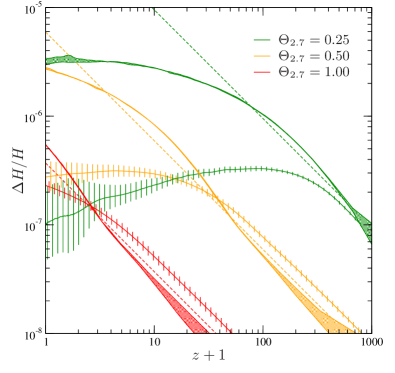
Figure 1: The perturbation of the Hubble rate from backreaction for different values of $\Theta_{2.7}$ in Einstein–de Sitter universes. The solid lines with error bars show the ensemble average and realization scatter for plane-symmetric relativistic simulations, whereas the shaded areas show the post-Newtonian estimate obtained from three 3D Newtonian N-body simulations. The latter is based on the estimate on the average kinetic and potential energy of the particles, the size of the shaded regions giving a rough indication for the uncertainty which is mainly caused by numerical deviations from the energy constraint, i.e. the Layzer-Irvine equation. Dashed lines are the prediction from second order perturbation theory. For $\Theta_{2.7}=0.25$ the backreaction $\Delta H/H$ stabilizes roughly around $z_{\rm st}\simeq 55$ while for $\Theta_{2.7}=0.5$ this happens at $z_{\rm st}\simeq 2.5$. Note that for $\Theta_{2.7}=1$ the time of stabilization is actually in the future, $z_{\rm st}<0$. In the 1D simulations the stabilization occurs earlier and at a lower amplitude.

In Fig. 1 we plot the perturbation of the Hubble parameter as a function of redshift for different values of $\Theta_{2.7}$ which is related to the equality scale by $k_{\rm eq}(\Theta_{2.7})=\Theta_{2.7}^{-2}k_{\rm eq}(1)$. In order not to mistake the effects from non-linearities by those of a cosmological constant, which leads to a decay of the gravitational potential due to the more rapid expansion, we have simulated pure flat matter models (Einstein–de Sitter). For $\Theta_{2.7}=1$ we have $k_{\rm eq}(1)={\cal H}_{\rm eq}(1)=2H_{0}\Omega_{r}^{-1/2}=0.1h^{2}/$Mpc and $1+z_{\rm eq}(\Theta_{2.7})=(1+z_{\rm eq}(1))\Theta_{2.7}^{-4}$. Assuming that clustering leads to the stabilization of $\Delta H/H=-\Phi_{0}^{\prime}/\mathcal{H}$, we expect that the redshift when this happens is proportional to $z_{\rm eq}$ and therefore scales as $\Theta_{2.7}^{-4}$. This is reasonably well verified in Fig. 1.

As further indication for the progress of structure formation we plot in Fig. 2 the mass fraction of the particles which are contained in regions where $n$ velocity streams overlap. For $n>1$ this means that shell crossing has occurred and structure formation has entered the non-linear regime. Fig. 2 shows that this happens around $z\sim 200$ for $\Theta_{2.7}=0.25$ while shell crossing only becomes relevant at $z\sim 3$ for the simulations with $\Theta_{2.7}=1$.

We also studied the impact of the UV cutoff, which is implemented in the simulations because of their finite resolution. The amplitude of the backreaction effect $\Delta H/H$ increases slightly with better mass resolution, but the dependence on the cutoff is very mild.

The results shown in Fig. 1 for the 3D case are from three simulations with $512^{3}$ particles. In the plane symmetric case we are able to vary the cutoff in a much larger range, and the results shown are fully converged. In this case, the large scatter between realizations is caused by the finite volume. Fluctuations are enhanced by the fact that, as opposed to 3D, there exists only a single mode for each given $k$. It should be noted that the realization scatter (i.e. cosmic variance) is not insignificant also in 3D. In particular, we find that it is larger than other effects, e.g. the influence of mass resolution, gravitational softening length and other simulation parameters.

Our interpretation of these findings is that once ‘stable clustering’ is established and most structures have formed and decoupled from the Hubble flow, the Hubble flow just proceeds (nearly) as before and the structures on small scales are irrelevant. On larger scales, structure formation is still ongoing and the virial limit is only reached asymptotically.

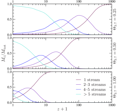
Figure 2: As structure formation proceeds, more and more mass is accumulated in non-linear structures. The figure shows the evolution with time of the fraction of mass which resides in regions which contain $n$ velocity streams for the plane symmetric simulations. For $n>1$ these regions have undergone shell crossing and this fraction is zero initially, since at the beginning the matter perturbations are fully in the linear regime. Perturbation theory is expected to be a poor description when a significant proportion ($\sim 50\%$, say) of the matter is in regions which contain more than one stream.

Discussion and conclusions

We have shown that, contrary to the expectations from perturbation theory, clustering does not induce large changes in the expansion rate. The contribution to backreaction from a given scale decays once the scale has entered the regime of stable clustering, i.e. once the non-linear structures have virialized. In the real Universe, this stable clustering progresses to larger and larger scales as time goes on until the Universe becomes $\Lambda$-dominated, after which linear perturbations no longer grow and no further scales enter the non-linear regime.

This result indicates that backreaction never becomes large, as the formation of non-linear structures does not accelerate the deviation from the averaged behavior on large scales. Instead backreaction appears to be reduced with the onset of non-linear structure formation. If this behavior of the perturbed Hubble rate is representative, relativistic backreaction effects, while certainly being present and non-negligible for precision cosmology with future large surveys, cannot explain the observed accelerated expansion of the Universe.

Although our results and arguments are suggesting strongly that backreaction does not significantly affect the background, they are not yet fully conclusive. Two areas especially need improvement. Firstly, we have not yet run a fully relativistic 3D simulation. Instead we used a relativistic plane-symmetric simulation and in addition computed the metric and relativistic effects based on the particle phase-space distribution from a standard 3D Newtonian N-body simulation. Although the results from the two approaches agree qualitatively, it would be desirable to repeat the analysis with a relativistic 3D simulation. We are planning to accomplish this task in the future. Secondly, it would be preferable to consider directly observables like distances to quantify the impact of backreaction.

References

- (1) T. H.-C. Lu, K. Ananda, C. Clarkson, and R. Maartens, “The cosmological background of vector modes,” JCAP 0902 (2009) 023, arXiv:0812.1349 [astro-ph].
- (2) S. R. Green and R. M. Wald, “A new framework for analyzing the effects of small scale inhomogeneities in cosmology,” Phys.Rev. D83 (2011) 084020, arXiv:1011.4920 [gr-qc].
- (3) N. E. Chisari and M. Zaldarriaga, “Connection between Newtonian simulations and general relativity,” Phys.Rev. D83 (2011) 123505, arXiv:1101.3555 [astro-ph.CO].
- (4) C. Clarkson, G. Ellis, J. Larena, and O. Umeh, “Does the growth of structure affect our dynamical models of the universe? The averaging, backreaction and fitting problems in cosmology,” Rept.Prog.Phys. 74 (2011) 112901, arXiv:1109.2314 [astro-ph.CO].
- (5) S. R. Green and R. M. Wald, “Newtonian and Relativistic Cosmologies,” Phys.Rev. D85 (2012) 063512, arXiv:1111.2997 [gr-qc].
- (6) J. Adamek, D. Daverio, R. Durrer, and M. Kunz, “General Relativistic N-body simulations in the weak field limit,” Phys.Rev. D88 (2013) 103527, arXiv:1308.6524 [astro-ph.CO].
- (7) J. Adamek, R. Durrer, and M. Kunz, “N-body methods for relativistic cosmology,” Class.Quant.Grav. 31 no. 23, (2014) 234006, arXiv:1408.3352 [astro-ph.CO].
- (8) M. Bruni, D. B. Thomas, and D. Wands, “Computing General Relativistic effects from Newtonian N-body simulations: Frame dragging in the post-Friedmann approach,” arXiv:1306.1562 [astro-ph.CO].
- (9) C. Bonvin, R. Durrer, and M. A. Gasparini, “Fluctuations of the luminosity distance,” Phys.Rev. D73 (2006) 023523, arXiv:astro-ph/0511183 [astro-ph].
- (10) C. Bonvin, R. Durrer, and M. Kunz, “The dipole of the luminosity distance: a direct measure of h(z),” Phys.Rev.Lett. 96 (2006) 191302, arXiv:astro-ph/0603240 [astro-ph].
- (11) I. Ben-Dayan, M. Gasperini, G. Marozzi, F. Nugier, and G. Veneziano, “Do stochastic inhomogeneities affect dark-energy precision measurements?,” Phys.Rev.Lett. 110 (2013) 021301, arXiv:1207.1286 [astro-ph.CO].
- (12) O. Umeh, C. Clarkson, and R. Maartens, “Nonlinear general relativistic corrections to redshift space distortions, gravitational lensing magnification and cosmological distances,” arXiv:1207.2109 [astro-ph.CO].
- (13) I. Ben-Dayan, M. Gasperini, G. Marozzi, F. Nugier, and G. Veneziano, “Average and dispersion of the luminosity-redshift relation in the concordance model,” arXiv:1302.0740 [astro-ph.CO].
- (14) O. Umeh, C. Clarkson, and R. Maartens, “Nonlinear relativistic corrections to cosmological distances, redshift and gravitational lensing magnification. II - Derivation,” arXiv:1402.1933 [astro-ph.CO].
- (15) C. Clarkson, O. Umeh, R. Maartens, and R. Durrer, “What is the distance to the CMB? How relativistic corrections remove the tension with local H0 measurements,” arXiv:1405.7860 [astro-ph.CO].
- (16) T. Buchert and S. Rasanen, “Backreaction in late-time cosmology,” Ann.Rev.Nucl.Part.Sci. 62 (2012) 57–79, arXiv:1112.5335 [astro-ph.CO].
- (17) N. Mustapha, B. A. Bassett, C. Hellaby, and G. F. R. Ellis Class. Quant. Grav. 15 (1998) 2363, arXiv:gr-qc/9708043 [gr-qc].
- (18) P. Bull and T. Clifton Phys. Rev. D 85 (2012) 103512, arXiv:1203.4479 [astro-ph.CO].
- (19) E. Di Dio, M. Vonlanthen, and R. Durrer, “Back Reaction from Walls,” JCAP 1202 (2012) 036, arXiv:1111.5764 [astro-ph.CO].
- (20) E. Di Dio and R. Durrer, “Vector and tensor contributions to the luminosity distance,” Phys. Rev. D 86 no. 2, (July, 2012) 023510, arXiv:1205.3366 [astro-ph.CO].
- (21) T. Buchert and M. Carfora, “Cosmological parameters are dressed,” Phys.Rev.Lett. 90 (2003) 031101, arXiv:gr-qc/0210045 [gr-qc].
- (22) T. Buchert, M. Kerscher, and C. Sicka, “Back reaction of inhomogeneities on the expansion: The Evolution of cosmological parameters,” Phys.Rev. D62 (2000) 043525, arXiv:astro-ph/9912347 [astro-ph].
- (23) T. Buchert, “Dark Energy from Structure: A Status Report,” Gen.Rel.Grav. 40 (2008) 467–527, arXiv:0707.2153 [gr-qc].
- (24) S. Rasanen, “Applicability of the linearly perturbed FRW metric and Newtonian cosmology,” Phys.Rev. D81 (2010) 103512, arXiv:1002.4779 [astro-ph.CO].
- (25) S. Rasanen, “Backreaction: directions of progress,” Class.Quant.Grav. 28 (2011) 164008, arXiv:1102.0408 [astro-ph.CO].
- (26) C. Wetterich, “Can structure formation influence the cosmological evolution?,” Phys.Rev. D67 (2003) 043513, arXiv:astro-ph/0111166 [astro-ph].
- (27) Planck Collaboration Collaboration, P. Ade et al., “Planck 2013 results. XVI. Cosmological parameters,” arXiv:1303.5076 [astro-ph.CO].
- (28) D. J. Eisenstein and W. Hu, “Power spectra for cold dark matter and its variants,” Astrophys.J. 511 (1997) 5, arXiv:astro-ph/9710252 [astro-ph].
- (29) D. J. Eisenstein and W. Hu, “Baryonic features in the matter transfer function,” Astrophys.J. 496 (1998) 605, arXiv:astro-ph/9709112 [astro-ph].
- (30) E. R. Siegel and J. N. Fry, “The Effects of Inhomogeneities on Cosmic Expansion,” ApJ 628 (July, 2005) L1–L4, astro-ph/0504421.
- (31) E. W. Kolb, S. Matarrese, A. Notari, and A. Riotto, “Effect of inhomogeneities on the expansion rate of the universe,” Phys. Rev. D 71 no. 2, (Jan., 2005) 023524, hep-ph/0409038.
- (32) E. W. Kolb, S. Matarrese, and A. Riotto, “On cosmic acceleration without dark energy,” New Journal of Physics 8 (Dec., 2006) 322, astro-ph/0506534.
- (33) A. Notari, “Late Time Failure of Friedmann Equation,” Modern Physics Letters A 21 (2006) 2997–3007, astro-ph/0503715.
- (34) N. Li and D. J. Schwarz, “Onset of cosmological backreaction,” Phys. Rev. D 76 no. 8, (Oct., 2007) 083011, gr-qc/0702043.
- (35) J. Behrend, I. A. Brown, and G. Robbers, “Cosmological backreaction from perturbations,” J. Cosmology Astropart. Phys 1 (Jan., 2008) 13, arXiv:0710.4964.
- (36) N. Li and D. J. Schwarz, “Scale dependence of cosmological backreaction,” Phys. Rev. D 78 no. 8, (Oct., 2008) 083531, arXiv:0710.5073.
- (37) C. Clarkson, K. Ananda, and J. Larena, “Influence of structure formation on the cosmic expansion,” Phys. Rev. D 80 no. 8, (Oct., 2009) 083525, arXiv:0907.3377 [astro-ph.CO].
- (38) O. Umeh, J. Larena, and C. Clarkson, “The Hubble rate in averaged cosmology,” J. Cosmology Astropart. Phys 3 (Mar., 2011) 29, arXiv:1011.3959 [astro-ph.CO].
- (39) C. Clarkson and O. Umeh, “Is backreaction really small within concordance cosmology?,” Classical and Quantum Gravity 28 no. 16, (Aug., 2011) 164010, arXiv:1105.1886 [astro-ph.CO].
- (40) W. Irvine PhD Thesis (1961) .
- (41) D. Layzer, “A Preface to Cosmogony. I. The Energy Equation and the Virial Theorem for Cosmic Distributions.,” ApJ 138 (July, 1963) 174.
- (42) V. Springel, S. D. White, A. Jenkins, C. S. Frenk, N. Yoshida, et al., “Simulating the joint evolution of quasars, galaxies and their large-scale distribution,” Nature 435 (2005) 629–636, arXiv:astro-ph/0504097 [astro-ph].
- (43) V. Springel, “The Cosmological simulation code GADGET-2,” Mon.Not.Roy.Astron.Soc. 364 (2005) 1105–1134, arXiv:astro-ph/0505010 [astro-ph].
- (44) V. Springel, N. Yoshida, and S. D. White, “GADGET: A Code for collisionless and gasdynamical cosmological simulations,” New Astron. 6 (2001) 79, arXiv:astro-ph/0003162 [astro-ph].