Fidelity at Berezinskii-Kosterlitz-Thouless quantum phase transitions

Abstract

We clarify the long-standing controversy concerning the behavior of the ground state fidelity in the vicinity of a quantum phase transition of the Berezinskii-Kosterlitz-Thouless type in one-dimensional systems. Contrary to the prediction based on the Gaussian approximation of the Luttinger liquid approach, it is shown that the fidelity susceptibility does not diverge at the transition, but has a cusp-like peak $\chi_{c}-\chi(\lambda)\sim\sqrt{|\lambda_{c}-\lambda|}$, where $\lambda$ is a parameter driving the transition, and $\chi_{c}$ is the peak value at the transition point $\lambda=\lambda_{c}$. Numerical claims of the logarithmic divergence of fidelity susceptibility with the system size (or temperature) are explained by logarithmic corrections due to marginal operators, which is supported by numerical calculations for large systems.

I Introduction

The ground state fidelity ZanardiPaunkovic06 ; VenutiZanardi07 ; You+07 , a concept stemming from quantum information theory, is the overlap amplitude $F(\lambda,\lambda+\delta\lambda)=|\langle\psi_{0}(\lambda)|\psi_{0}(\lambda+\delta\lambda)\rangle|$ between two ground state wave functions of the Hamiltonian $\hat{\mathcal{H}}(\lambda)=\hat{\mathcal{H}}_{0}+\lambda\hat{V}$ at different values of the coupling parameter $\lambda$. It is widely used as an unbiased indicator of quantum phase transitions You+07 ; VenutiZanardi07 ; Schwandt+09 ; Gu10rev , especially in one-dimensional (1D) systems where a very accurate numerical calculation of the ground state wave function is possible thanks to the well-developed density matrix renormalization group (DMRG) technique White ; Uli . Hereafter, we restrict the discussion to the 1D case.

Fidelity vanishes exponentially with the system size $L$. The fidelity susceptibility per site (FS)

$$\chi_{L}=(1/L)\lim_{\delta\lambda\to 0}\big{[}-2\ln F(\lambda,\lambda+\delta\lambda)\big{]}/(\delta\lambda)^{2}$$

is an intensive quantity expected to diverge in the thermodynamic limit $L\to\infty$ at the phase transition point $\lambda=\lambda_{c}$ due to nonanalyticity in the ground state. For finite $L$, this divergence translates into a presence of a peak in $\chi_{L}(\lambda)$ at $\lambda=\lambda_{*}$, with $\lambda_{*}\to\lambda_{c}$ and $\chi_{L}(\lambda_{*})\to\infty$ at $L\to\infty$. Assuming a translational invariant system with the unique ground state, perturbed by a local operator $\hat{V}=\partial_{\lambda}\hat{\mathcal{H}}=\sum_{x}\hat{V}(x)$, one obtains VenutiZanardi07 the following connection

$$\chi_{L}=\int_{a}^{L}dx\int_{0}^{\infty}d\tau\,\tau G(x,\tau),$$ (1)

between the FS and the reduced correlation function $G(x,\tau)=\langle\!\langle\hat{V}(x,\tau)\hat{V}(0,0)\rangle\!\rangle\equiv\langle\hat{V}(x,\tau)\hat{V}(0,0)\rangle-\langle\hat{V}(0,0)\rangle^{2},$ where the imaginary time evolution is defined by $\hat{V}(x,\tau)=e^{\tau\hat{\mathcal{H}}}\hat{V}(x)e^{-\tau\hat{\mathcal{H}}}$, averages are taken in the ground state $|\psi_{0}(\lambda)\rangle$, and $a$ is the short-range (lattice) cutoff. Expression (1) diverges at $L\to\infty$ as $\chi\propto L^{1+2z-2\Delta_{V}}$, where $\Delta_{V}$ is the scaling dimension of $\hat{V}(x)$ at the critical point and $z$ is the dynamic exponent, as long as $\Delta_{V}<z+1/2$. At $\Delta_{V}=z+1/2$ there is only a logarithmic divergence GuLin09 , and with the further increase of $\Delta_{V}$ the FS remains finite at the critical point.

II Controversy

The above arguments VenutiZanardi07 show that the FS must be insensitive not only against marginal and irrelevant perturbations ($\Delta_{V}\geq z+1$), but even against relevant perturbations with $z+1/2<\Delta_{V}<z+1$. In the case of the Berezinskii-Kosterlitz-Thouless (BKT) phase transition, $z=1$ and $\Delta_{V}=2$, so it has been initially concluded You+07 ; VenutiZanardi07 ; Chen+08 that transitions of this type cannot be detected by means of the finite-size scaling analysis of the FS. A prominent example of the BKT transition is the transition at the isotropic point $\lambda=1$ in the so-called XXZ spin-$\frac{1}{2}$ chain defined by the Hamiltonian

$$\hat{\mathcal{H}}_{XXZ}=\sum_{n}\Big{\{}S^{x}_{n}S^{x}_{n+1}+S^{y}_{n}S^{y}_{n+1}+\lambda S^{z}_{n}S^{z}_{n+1}\Big{\}},$$ (2)

where $S^{a}_{n}$ are spin-$\frac{1}{2}$ operators at site $n$.

This conclusion has been apparently defeated by Yang MFYang07 and Fjærestad Fjarestad08 . Their approach uses the fact that the low-energy effective theory of the model (2) (as well as of many other gapless 1D systems), obtained by the Abelian bosonization Giamarchi-book , is the so-called Luttinger liquid (LL) described by the Hamiltonian

$$\mathcal{H}_{\rm eff}=\frac{v}{2}\int dx\Big{\{}K\Pi^{2}+\frac{1}{K}(\partial_{x}\Phi)^{2}\Big{\}},$$ (3)

where $\Phi$ is the compact bosonic field ($\Phi=\Phi+\sqrt{\pi}$), and $\Pi$ is its conjugate momentum. The velocity $v=v(\lambda)$ and the LL parameter $K=K(\lambda)$ are generally functions of the original coupling $\lambda$ that have to be obtained as fixed points of the renormalization group (RG) flow equations. Alternatively, they can be extracted from the knowledge of exact long-distance behavior of correlation functions. For the XXZ model (2), exact correlator asymptotics is known from the Bethe ansatz, which yields $K=\pi/[2(\pi-\arccos\lambda)]$ and $v=\pi\sqrt{1-\lambda^{2}}/(2\arccos\lambda)$ JohnsonKrinskyMcCoy73 . Since the effective model (3) is quadratic, one can explicitly calculate the fidelity $F(K,K+\delta K)$ and obtain for the FS in the thermodynamic limit

$$\chi|_{L=\infty}=(\partial_{\lambda}K)^{2}/(8aK^{2}).$$ (4)

The dependence $K(\lambda)$ is singular at $\lambda=1$, which leads to the divergence of the FS $\chi\propto(1-\lambda)^{-1}$.

This direct calculation of overlaps might seem questionable since the connection between the wave functions of the initial model and its fixed-point low-energy theory is not so clear. Instead, one can use an alternative derivation due to Sirker Sirker10 based on the relation (1). Indeed, using the effective Hamiltonian (3), the perturbation $\hat{V}=\partial_{\lambda}\hat{\mathcal{H}}$ can be represented as

$$\hat{V}=\frac{\partial_{\lambda}v}{v}\hat{\mathcal{H}}(\lambda)+\frac{v\partial_{\lambda}K}{2K}\int dx\,\hat{W}(x),$$ (5)

where

$$\hat{W}(x)=K\Pi^{2}-\frac{1}{K}(\partial_{x}\Phi)^{2}.$$ (6)

The first term in (5) commutes with $\hat{\mathcal{H}}(\lambda)$ and thus gives no contribution into $\chi_{L}$ note1-temp , but the second term contributes the prefactor leading exactly to the form (4). The scaling dimension of the second term is $\Delta_{W}=2$, so the correlator in (1) behaves as

$$G(x,\tau)\sim A(\lambda)v^{2}(x^{2}+v^{2}\tau^{2})^{-2},$$ (7)

the integral in (1) is finite at $L\to\infty$, and the divergence originates solely from the prefactor.

One can show that this singular behavior of $K(\lambda)$ is a generic property of any BKT transition. The general theory of a BKT transition is given by the Hamiltonian (3) perturbed by the cosine term $-(u/a^{2})\cos(\sqrt{16\pi}\Phi)$, where $a$ is the lattice cutoff and $u$ is the dimensionless coupling. The proximity to the transition is controlled by the parameter $(\lambda_{c}-\lambda)\approx K-1/2-\pi u/2$. It follows from the RG equations Kosterlitz74 ; PelissettoVicari13 that in the thermodynamic limit the fixed point behavior is $K-1/2\approx\sqrt{\pi u(\lambda_{c}-\lambda)}$, so the FS diverges. In a finite system, however, the RG flow should be stopped at the RG scale $l\propto\ln(L/a)$, and the derivative of $K$ behaves as $(\partial K/\partial\lambda)\approx(4\pi u/3)l$ at $l\to\infty$, so according to (4) the FS at the transition should scale as

$$\chi_{L}\propto u^{2}\ln^{2}(L/a).$$ (8)

Indeed, numerical results show that in the vicinity of the isotropic point the FS exhibits a peak WangFengChen10 located at $\lambda>1$, which moves very slowly towards $\lambda=1$ with increasing $L$, and whose height grows with $L$ much faster than corrections in powers of $1/L$ could explain note-wang . A similar behavior has been reported Sirker10 for the finite-temperature FS, and the results were claimed to be consistent with the $\ln^{2}(T_{0}/T)$ behavior, essentially of the same origin as Eq. (8) (in the case of an infinite system at finite temperature, the RG flow is stopped at the scale $l\sim\ln(T_{0}/T)$ where $T_{0}$ is some nonuniversal energy scale of the order of the spin exchange energy). Recently, for the XXZ chain a divergent FS similar to (4) has been claimed LangariRezakhani12 on the basis of the real-space quantum renormalization group. On the other hand, other authors did not see any divergence in the FS at BKT-type transitions in the spin-$\frac{1}{2}$ XXZ chain Chen+08 and in bosonic Hubbard model Carrasquilla+13 ; Damski14 . Further, comparison of the FS calculated according to (4) with the numerical results shows Sirker10 that in order to fit the data one has to assume the ultraviolet cutoff $a$ to be strongly $\lambda$-dependent even in the vicinity of the free fermion point $\lambda=0$. This controversy is aggravated by the fact that a logarithmic growth is difficult to distinguish numerically from the well known logarithmic finite-size corrections at the BKT transitions.

III Resolution of Controversy

There is a subtle problem with the above derivation of a diverging FS, immediately revealed by a closer look at the representation (5): recalling the original model (2), we see that $\hat{V}=\sum_{n}S^{z}_{n}S^{z}_{n+1}$, so $\hat{V}(x)$ is a bounded operator, while in Eq. (5) the bounded operator $\hat{W}(x)$ carries a prefactor that diverges at $\lambda\to 1$ independently of any ultraviolet cutoff. This indicates that the divergence might be an artefact of the effective representation (5), built on the Abelian bosonization and becoming inapplicable in the vicinity of the transition point. A similar problem is known for the amplitudes of correlation functions calculated by Lukyanov Lukyanov99 : the amplitudes explode at $\lambda\to 1$, meaning that the applicability of the correspondent asymptotics is pushed to larger and larger distances. The integral (1) is convergent at $L\to\infty$, so divergences coming from such prefactors may be compensated by terms neglected in Eq. (3).

Generally, one should not rely on divergences stemming from prefactors of operators of the fixed point action (action where we neglect all irrelevant terms in particular those that may and will lead to cancellation of these spurious divergences in physical quantities). However, infrared divergences due to the correlators of the fixed point action are physical, since irrelevant terms, being ’harmless’ at long distances, can not compensate them.

Assuming, from the boundedness of $\hat{V}(x)$, that the amplitude $A(\lambda)$ in the correlator (7) remains finite at $\lambda\to 1$, one returns to the initial conclusion that the FS at the transition stays finite as well. Finite-size corrections to $\chi$ might be naively estimated in a standard way by exploiting the conformal symmetry: substitution $(x\pm iv\tau)\mapsto(L/\pi)\sinh\left[\frac{\pi}{L}(v\tau\pm ix)\right]$ in the correlator (7), mapping infinite space-time onto a stripe, yields

$$\chi_{L}=\chi_{0}(\lambda)\big{[}1-\frac{\pi a}{L}+O(L^{-2})\big{]},\quad\chi_{0}(\lambda)\sim\frac{\pi A(\lambda)}{2a}.$$ (9)

Although numerical results VenutiZanardi07 ; Chen+08 ; LangariRezakhani12 for the model (2) in the gapless phase $|\lambda|<1$ are indeed consistent with (9), this type of finite-size scaling certainly breaks down close to the observed peak in the FS VenutiZanardi07 ; Chen+08 ; WangFengChen10 . The logarithmic modification of the correlator $G(x,0)\mapsto\ln^{\alpha}(x)G(x,0)$, which can take place at the isotropic point $\lambda=1$, would affect the finite-size corrections in (9) only by changing them from $L^{-1}$ to $L^{-1}\ln^{\alpha}(L)$, not solving the problem.

To obtain the correct finite-size scaling of $\chi$ close to the SU(2)-symmetric BKT transition point $\lambda=1$, it is convenient to use non-Abelian bosonization Affleck85 .

In non-Abelian approach, the low-energy theory of the model (2) is described by the Hamiltonian

$$\!\!\mathcal{H}=\!\mathcal{H}_{\rm WZW}-\!\!\int\!\!\frac{dx}{2\pi}\Big{\{}g_{\parallel}J_{0}\bar{J}_{0}+\frac{g_{\bot}}{2}(J_{+}\bar{J}_{-}\!+\!J_{-}\bar{J}_{+}\!)\!\Big{\}},$$ (10)

where $\mathcal{H}_{\rm WZW}$ corresponds to level $k=1$ SU(2) Wess-Zumino-Witten (WZW) theory DiFrancesco ,

$$\mathcal{H}_{\rm WZW}=\frac{2\pi v}{3}\int dx\Big{\{}:\bm{J}\cdot\bm{J}:+:\bm{\bar{J}}\cdot\bm{\bar{J}}:\Big{\}},$$ (11)

and the second term in (10) describes marginal current-current perturbation. Here $\bm{J}$ and $\bm{\bar{J}}$ are the currents of left- and right-movers, which are holomorphic functions of the complex coordinates $z=x+iv\tau$ and $z^{*}$, respectively, and $:\ldots:$ denotes normal ordering. Currents satisfy the Kac-Moody algebra

$$[J^{a}(z),J^{b}(z^{\prime})]=\frac{i}{2\pi}\delta_{ab}\delta^{\prime}(z-z^{\prime})+i\varepsilon_{abc}J^{c}(z)\delta(z-z^{\prime}),$$ (12)

and their two-point correlation functions evaluated with the unperturbed WZW fixed point action (in an infinite-size system) are given by

$$\langle J^{a}(z)J^{b}(0)\rangle=\frac{\delta_{ab}}{4\pi^{2}|z|^{2}},\quad\langle J^{a}(z)\bar{J}^{b}(z^{\prime})\rangle=0.$$ (13)

For finite system size $L$ the first correlator in Eq. (13) gets modified by the conformal substitution $z\mapsto\frac{L}{\pi}\sin(\frac{\pi z}{L})$ and the second equation of Eq. (13) gets modified into $\langle J^{a}(z)\bar{J}^{b}(z^{\prime})\rangle\propto\frac{1}{L^{2}}$. The cartesian and spherical components of the currents are connected in a standard way, $J_{\pm}=J^{x}\pm iJ^{y}$, $J_{0}=J^{z}$.

Running couplings $g_{\parallel}$ and $g_{\bot}$ are governed by the following BKT-type RG equations Zamolodchikov :

$$\frac{dg_{\parallel}}{dl}=-\frac{2g_{\bot}^{2}}{2-g_{\parallel}},\quad\frac{dg_{\bot}}{dl}=-\frac{2g_{\parallel}g_{\bot}}{2-g_{\parallel}},$$ (14)

where $l$ is the RG scale.

Figure 1: Diagrams for the current correlators contributing to $\chi_{0}$ (a) and $\chi_{1}$ (b), see Eqs. (18), (20), with continuous and dashed lines indicating left- and right-movers, respectively.

The fidelity-changing perturbation $\hat{V}=\sum_{n}S^{z}_{n}S^{z}_{n+1}$ can be represented as

$$\hat{V} = \lambda^{-1}\Big{\{}\hat{\mathcal{H}}_{XXZ}-\sum_{n}(S^{x}_{n}S^{x}_{n+1}+S^{y}_{n}S^{y}_{n+1})\Big{\}}$$ (15)

$$\mapsto \lambda^{-1}\mathcal{H}-\int dx\hat{O}(x,\tau),$$

where

$$\hat{O}(x,\tau)\sim(J_{+}+\bar{J}_{+})(J_{-}+\bar{J}_{-})+\text{h.c.}$$ (16)

One can evaluate the correlator $G(x,\tau)=\langle\!\langle\hat{O}(x,\tau)\hat{O}(0,0)\rangle\!\rangle$ in the perturbed WZW model (10), and calculate the fidelity susceptibility $\chi_{L}=\int_{a}^{L}dx\int_{0}^{\infty}d\tau\,\tau G(x,\tau)$, to the lowest order in the couplings $g_{\parallel}$, $g_{\bot}$. Doing so, one obtains

$$\chi_{L}=\chi_{0}-g_{\parallel}\chi_{1}+O(g_{\parallel}^{2},g_{\bot}^{2}),$$ (17)

where $\chi_{0}$, $\chi_{1}$ are finite positive constants discussed below.

The “unperturbed” value $\chi_{0}$ of the FS (i.e., without taking into account corrections due to marginal operators) is determined by the four-current correlators (see the diagram shown in Fig. 1(a)), that factorize into a product of two-point functions such as $\langle\!\langle J_{+}(z)J_{-}(0)\rangle\!\rangle\langle\!\langle\bar{J}_{-}(z)\bar{J}_{+}(0)\rangle\!\rangle$,

$$\chi_{0}\propto\int\frac{\tau\theta(\tau)\,d^{2}z}{|z|^{4}}>0.$$ (18)

Above we have used the infinite-size current correlators (13). The constant $\chi_{0}$ here coincides with $\chi_{0}(\lambda=1)$ in Eq. (9). If one takes the finite-size corrections into account by correcting current-current correlators (13) with the help of the conformal substitution $z\mapsto\frac{L}{\pi}\sin(\frac{\pi z}{L})$, the value $\chi_{0}$ gets modified according to

$$\chi_{0}\mapsto\chi_{0}\Big{(}1-{\pi a/}{L}\Big{)}+O(1/L^{2}).$$ (19)

The other constant

$$\chi_{1}\propto\int\frac{\tau\theta(\tau)\,d^{2}z\,d^{2}z^{\prime}}{|z|^{2}|z^{\prime}|^{2}|z-z^{\prime}|^{2}}>0$$ (20)

is determined by six-current correlators that correspond to three-point functions Affleck+89 of the marginal operator $\hat{O}$, such as $\langle\!\langle J_{+}(z)J_{0}(z^{\prime})J_{-}(0)\rangle\!\rangle\langle\!\langle\bar{J}_{-}(z)\bar{J}_{0}(z^{\prime})\bar{J}_{+}(0)\rangle\!\rangle$ (see Fig. 1(b)).

III.1 Finite-size scaling

Combining Eqs. (17), (19), and the RG equations (14) we can determine the finite-size scaling of the FS in the vicinity of the BKT transition.

First we consider the scaling right at the transition, i.e., at the isotropic point. It is well known that finite-size corrections from marginal operators are only suppressed logarithmically Cardy86 ; Blote+86 ; Affleck86 ; Eggert+94 in the system size. Indeed, at the SU(2) point $\lambda=1$ one has $g_{\bot}=g_{\parallel}=g>0$, and for weak coupling the solution of RG equations simplifies to $g(l)\simeq 1/l$, where $l$ is the RG scale. In the spirit of Ref. Cardy86, , one can stop the RG flow at the length scale $l_{L}\sim\ln(L/a)$, and replace the running coupling $g(l)$ in Eq. (17) by its “RG-improved” value $g(l_{L})\sim 1/\ln(L/a)$ taken at this scale, which yields the following logarithmic finite-size scaling:

$$\chi_{L}\simeq\chi_{0}-\frac{\chi_{1}}{\ln(L/a)}+O\left[\frac{1}{\ln^{2}(L/a)}\right].$$ (21)

We expect such scaling of the FS to be valid at BKT transitions in other 1D models as well, since any BKT transition point exhibits an enhanced SU(2) symmetry.

Away from the SU(2) point inside the gapless region, log corrections in (21) get replaced by power laws. Indeed, close to the SU(2) point the running coupling in the leading correction to FS in Eq. (17) can be RG-improved as Lukyanov98 $g_{\parallel}(l_{L})-g^{*}\propto(a/L)^{8K-4}$, where the fixed point value of $g_{\parallel}$ is $g^{*}\equiv g_{\parallel}(l=\infty)=2-K^{-1}$. Thus, for $K<\frac{5}{8}$ ($\lambda>\cos\frac{\pi}{5}\approx 0.81$ in the XXZ chain) the leading contribution to the finite size scaling of $\chi_{L}$ is given by

$$\chi_{L}-\chi_{\infty}\sim-(a/L)^{8K-4},\quad K<5/8,$$ (22)

which transforms into log corrections in the SU(2) limit $K\to\frac{1}{2}$. For $K>\frac{5}{8}$, the above correction becomes subleading with respect to the $1/L$ terms stemming from (19), and thus the leading finite-size correction is

$$\chi_{L}-\chi_{\infty}\propto-(a/L),\quad K>5/8.$$ (23)

III.2 Finite-temperature corrections

The above analysis is easily carried over to the low-temperature behavior of FS. We adopt the definition of the finite-temperature FS Schwandt+09 based on (1) with ground state averages replaced by thermal ones, and the upper integration limit in $\tau$ set to $1/(2T)$. Perturbative corrections to the FS will be again determined by the formula (17), with the “RG-improved” couplings taken at the RG cutoff scale $l_{T}\sim\ln(T_{0}/T)$, where $T_{0}\sim v$ is some energy scale of the order of the exchange constant (set to unity in our Hamiltonian (2)).

Note that in this case the conformal substitution $z\mapsto\frac{v}{\pi T}\sinh\big{(}\frac{\pi Tz}{v}\big{)}$ in the correlator (7) leads only to quadratic finite-temperature corrections of the type $\chi-\chi_{0}\propto-T^{2}$. However, there is another contribution Sirker10 to the correlator stemming from the term in the perturbation that is proportional to the Hamiltonian (the first term in Eq. (5), or Eq. (15)). This contribution is proportional to the variance of the Hamiltonian, $\langle\mathcal{H}^{2}\rangle-\langle\mathcal{H}\rangle^{2}$, and while it vanishes exactly in the ground state (contrary to what is stated in Ref. Sirker10, ), the corresponding expression is nonzero in the case of thermal averages. This yields the following correction to the FS

$$\chi\mapsto\chi+\frac{c_{v}}{8}\Big{(}\frac{\partial_{\lambda}v}{v}\Big{)}^{2},$$ (24)

where $c_{v}=(\pi T/3v)$ is the specific heat of the model, so the correction is obviously positive and linear in $T$. So, in the finite-temperature case Eq. (24) can be viewed as being formally similar to Eq. (19), if one substitutes $a/L$ by $T/T_{0}$ (up to the change of sign of the correction).

In view of the above, the low-temperature behavior of the FS can be deduced from Eqs. (21)-(23) by means of the substitution $(a/L)\mapsto(T/T_{0})$. Particularly, at the isotropic point

$$\left.\chi(T)\right|_{L=\infty}-\chi_{0}\propto-1/\ln(T_{0}/T),\quad T\to 0.$$ (25)

Away from the SU(2) point, the leading low temperature correction to $\chi(T)|_{L=\infty}$ depends on $\lambda$: for $\lambda>\cos\frac{\pi}{5}$ the correction is negative,

$$\left.\chi(T)\right|_{L=\infty}-\chi_{0}\propto-(T/T_{0})^{8K-4},$$ (26)

while for $\lambda<\cos\frac{\pi}{5}$ it becomes positive,

$$\left.\chi(T)\right|_{L=\infty}-\chi_{0}\propto T.$$ (27)

Thus, the finite-temperature correction has to vanish at some value of $\lambda$ close to $\cos\frac{\pi}{5}$. This explains crossing of FS curves corresponding to different low temperatures at $\lambda\simeq\cos\frac{\pi}{5}$ in Fig. 4(a) of Ref. Sirker10, .

III.3 The FS behavior in the thermodynamic limit

Finally, we would like to discuss the shape of the FS curve $\chi_{L}(\lambda)$ in the vicinity of the BKT transition at $\lambda=\lambda_{c}$, in the thermodynamic limit $L\to\infty$. Right at the transition, the FS is finite, $\chi_{L\to\infty}(\lambda_{c})=\chi_{0}$. Off the transition point inside the gapped region, we can again use Eq. (17) to calculate the leading correction to the FS. In the gapped region, there is a finite correlation length $\xi\sim e^{B|\lambda-\lambda_{c}|^{-1/2}}$, where $B$ is some positive numerical factor, so for $L\gg\xi$ the RG flow gets stopped at the scale $l_{\xi}\sim\ln(\xi/a)$, and, similar to Eq. (21), we obtain the leading contribution as

$$\chi_{0}-\chi_{\rm gapped}(\lambda)\propto\frac{1}{l_{\xi}}\propto|\lambda-\lambda_{c}|^{1/2}.$$ (28)

We note that in the gapped region there is an additional factor $\exp\{-(x^{2}+v^{2}\tau^{2})^{1/2}/\xi\}$ in the correlator (7), but it only introduces a negligible (very smooth) modification of the FS in the vicinity of BKT point, since the correlation length diverges exponentially at the transition.

On the other side of the BKT transition, inside the gapless region, as we have already seen in Sec. III.1, the coupling $g_{\parallel}$ flows to the finite fixed point value $g^{*}=2-1/K$, and finite-size corrections vanish according to the power law $g_{\parallel}(l_{L})-g^{*}\propto(a/L)^{8K-4}$. Hence, in the thermodynamic limit $L\to\infty$ one has

$$\chi_{0}-\chi_{\rm gapless}(\lambda) \propto (2-1/K)\propto|\lambda-\lambda_{c}|^{1/2}.$$ (29)

Thus, in the thermodynamic limit, in the vicinity of the BKT transition, the FS exhibits a peak with the square-root cusp:

$$\chi_{L=\infty}(\lambda)=\chi_{0}-\alpha_{\pm}\sqrt{|\lambda-\lambda_{c}|},\quad\lambda\to\lambda_{c}\pm 0,$$ (30)

where $\alpha_{\pm}$ are some positive factors.

It should be mentioned that the cusp must be rather difficult to observe numerically: finite-size corrections tend to smoothen the cusp, so one has to study systems up to a sufficiently large size $L$. Another remark concerns the problem of defining the FS in the thermodynamic limit if the ground state is degenerate, as is the case, e.g., for the doubly degenerate Néel ground state of the XXZ chain in the gapped region. In the next section we, in addition to the XXZ chain, will consider two other models with the BKT transition that have unique gapped ground states.

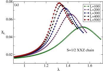
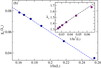
Figure 2: (Color online). (a) The fidelity susceptibility for spin-$\frac{1}{2}$ XXZ chain (2) of up to $L=500$ spins, as a function of the anisotropy $\lambda$; symbols denote DMRG results, and lines are guide to the eye. (b) The finite-size scaling of the peak position $\lambda_{*}$ and amplitude $\chi_{L}(\lambda_{*})$; lines are results of fits to (21) and (31), see text for details.

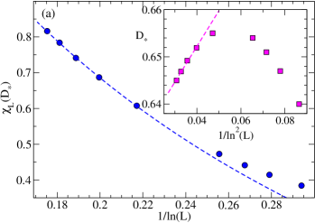
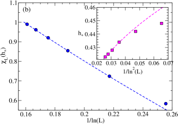
Figure 3: (Color online). (a) The finite-size scaling of the peak position $D_{*}$ and its value $\chi_{L}(D_{*})$, for the FS with respect to the single-ion anisotropy $D$ in the spin-$1$ chain model defined by the Hamiltonian (32) with $\theta=-0.85\pi$; (b) the same for the peak position $h_{*}$ and value $\chi_{L}(h_{*})$ of the FS with respect to the staggered field $h$ in the spin-$\frac{1}{2}$ anisotropic chain described by the model (33) at $\lambda=-0.9$. Symbols show numerical (DMRG) results, and lines are fits to scaling laws (21), (31).

IV Numerical results

To support our conclusions, we have performed DMRG calculations White ; Uli (in matrix product formulation Verstraete ) of the FS for the model (2), for large open chains of up to $L=500$ sites note-dmrg . The resulting FS as a function of $\lambda$ is shown in Fig. 2(a): as observed in previous studies for small systems, there is a peak with the height slowly growing and the position slowly converging with the increase of $L$. We start by fitting the finite-size dependence of the peak position $\lambda_{*}$ with the help of the ansatz

$$\lambda_{*}\simeq\lambda_{0}+\lambda_{1}/\ln^{2}(L/a)+\cdots,$$ (31)

which can be extracted by using standard scaling argumentsSchultkaManousakis94 on the gapped side of the BKT transition: since the infinite-system correlation length in the vicinity of the transition behaves as $\xi\propto ae^{-B/\sqrt{\lambda-\lambda_{c}}}$, Eq. (31) is obtained by postulating that $\xi\sim L$ at $\lambda\sim\lambda_{*}$. Further, when fitting the peak position $\lambda_{*}$ according to (31), we fix $\lambda_{0}=1$, which allows us to extract the cutoff $a$. Subsequently, we use the extracted value of the cutoff when fitting the peak value $\chi_{L}(\lambda_{*})$ of the FS according to our result (21). The results of those fits, shown in Fig. 2, demonstrate good agreement with the theory.

The above picture of non-diverging FS with strong logarithmic corrections due to marginal operators should be a generic feature of any BKT transition. To demonstrate that, we present here results of numerical studies for two more models containing such transitions. The first model is the anisotropic spin-1 chain defined by the Hamiltonian

$$\hat{\mathcal{H}}=\sum_{n}\{J_{1}^{\theta}(\bm{S}_{n}\cdot\bm{S}_{n+1})+J_{2}^{\theta}\big{(}\bm{S}_{n}\cdot\bm{S}_{n+1}\big{)}^{2}+D\big{(}S_{n}^{z}\big{)}^{2}\},$$ (32)

where $\bm{S}_{n}$ are spin-1 operators at site $n$, $J_{1}^{\theta}=\cos{\theta}$ and $J_{2}^{\theta}=\sin{\theta}$ are exchange constants, and $D>0$ is the single-ion anisotropy. For $\theta\in[-\frac{3\pi}{2},-\frac{3\pi}{4}]$, with the increase of $D$ this model exhibits a BKT transition from the gapless ferromagnetic XY phase to the gapped large-$D$ phase, recently studied Rodriguez+11 in the context of spinor bosons. Numerically, the FS as function of $D$ exhibits a slowly growing peak Rodriguez+11 , quite similar to the picture shown in Fig. 2(a). Here we extend the result of Ref. Rodriguez+11, to much larger systems note-selfpawn and show that the finite-size behavior of the peak height and position is consistent with the scaling formulas (21) and (31), see Fig. 3(a).

One more model corresponds to the spin-$\frac{1}{2}$ ferromagnetic anisotropic chain defined by the Hamiltonian (2) with $-1<\lambda<0$, perturbed by staggered field $h$:

$$\hat{\mathcal{H}}=\hat{\mathcal{H}}_{XXZ}+h\sum_{n}(-1)^{n}S_{n}^{z}.$$ (33)

For $-1<\lambda<-1/\sqrt{2}$, this model exhibits a BKT-type phase transition stag-xxz to a gapped antiferromagnetic phase at a finite value of the field $h$. Our DMRG calculations for the FS as function of $h$ show the same typical behavior of a slowly growing and poorly converging peak, and the finite-size scaling results presented in Fig. 3(b) show that the numerical data is again consistent with the scaling laws (21), (31).

V Summary

We have shown that FS does not diverge at Berezinskii-Kosterlitz-Thouless-type quantum phase transitions in one spatial dimension. Instead, it merely exhibits a finite-amplitude peak in the vicinity of the transition, with logarithmic finite-size scaling corrections of the form (21), (31) which are too easy to confuse numerically with a logarithmic growth of the peak. The same is true for the finite-temperature FS, which instead of the claimed Sirker10 divergence $\chi\propto\ln^{2}(T_{0}/T)$ at $T\to 0$ should contain log corrections of the form $\chi\simeq\chi_{0}-\chi_{1}/\ln(T_{0}/T)$.

The would-be divergence of the FS, originally proposed MFYang07 on the basis of mapping to Luttinger liquid (LL), and in the meantime enjoying the status of an established result Venuti+08 ; Sirker10 ; LangariRezakhani12 ; Rey , is an artefact due to the catastrophic shrinking of the applicability range for using the LL Gaussian effective description (3) when calculating the FS of the original microscopic model as one approaches the BKT transition. To identify the correct scaling of the FS with respect to some perturbation in a specific model at the BKT transition, it is crucial to properly identify perturbation in effective description that includes irrelevant corrections to the LL Guassian Hamiltonian beyond the mere renormalization of LL parameters.

From a more general viewpoint, the main message of this work is a warning about the naive use of the operator prefactors (”amplitudes”) of the effective action, obtained in the Abelian bosonization: one should not trust divergences stemming from such amplitudes, since they will be “healed” by the effects of irrelevant operators not taken into account in the fixed point action.

On the practical side, our results indicate that using the FS as a tool to detect BKT transitions (and especially to extract thermodynamic critical values of microscopic parameters) is extremely inconvenient, since the uncertainties of logarithmic fits remain too strong, even if one goes to the largest numerically tractable system sizes. Other detection methods suggested in quantum information theory, e.g., looking at discontinuities of fidelity WangChenLiZhou12 , or using bipartite fluctuations Rachel might be a better alternative.

- (1) P. Zanardi and N. Paunkovic, Phys. Rev. E 74, 031123 (2006).
- (2) L. Campos Venuti and P. Zanardi, Phys. Rev. Lett. 99, 095701 (2007).
- (3) W.-L. You, Y.-W. Li, and S.-J. Gu, Phys. Rev. E 76, 022101 (2007).
- (4) D. Schwandt, F. Alet, and S. Capponi, Phys. Rev. Lett. 103, 170501 (2009).
- (5) S.-J. Gu, Int. J. Mod. Phys. B 24, 4371 (2010).
- (6) S. R. White, Phys. Rev. Lett. 69, 2863 (1992).
- (7) U. Schollwöck, Rev. Mod. Phys. 77, 259 (2005); Ann. Phys. 326, 96 (2011).
- (8) S.-J. Gu and H.-Q. Lin, EPL 87, 10003 (2009).
- (9) S. Chen, L. Wang, Y. Hao, and Y. P. Wang, Phys. Rev. A 77, 032111 (2008).
- (10) M. F. Yang, Phys. Rev. B 76, 180403(R) (2007).
- (11) J. O. Fjærestad, J. Stat. Mech. P07011 (2008).
- (12) T. Giamarchi, Quantum physics in one dimension (Oxford University Press, Oxford 2003).
- (13) J. D. Johnson, S. Krinsky, and B. McCoy, Phys. Rev. A 8, 2526 (1973).
- (14) J. Sirker, Phys. Rev. Lett. 105, 117203 (2010).
- (15) This term does contribute to the finite-temperature FS, see Ref. Sirker10, , but its contribution vanishes exactly for the ground state FS even in finite-size systems, contrary to the statement in Ref. Sirker10, .
- (16) J. M. Kosterlitz, J. Phys. C 7, 1046 (1974).
- (17) A. Pelissetto and E. Vicari, Phys. Rev. E 87, 032105 (2013).
- (18) B. Wang, M. Feng, and Z.-Q. Chen, Phys. Rev. A 81, 064301 (2010).
- (19) The authors of Ref. WangFengChen10 attempted a power-law fitting of the FS which resulted in an anomalously low power usually indicating the presence of log corrections.
- (20) A. Langari and A. T. Rezakhani, New J. Phys. 14, 053014 (2012).
- (21) J. Carrasquilla, S. R. Manmana, and M. Rigol, Phys. Rev. A 87, 043606 (2013).
- (22) M. Lacki, B. Damski, and J. Zakrzewski, Phys. Rev. A 89, 033625 (2014).
- (23) S. Lukyanov, Phys.Rev. B 59, 11163 (1999).
- (24) I. Affleck, Phys. Rev. Lett. 55, 1355 (1985).
- (25) P. Di Francesco, P. Mathieu, and D. Sénéchal, Conformal Field Theory (Springer, New York 1997).
- (26) Al. B. Zamolodchikov, Int. J. Mod. Phys. A 10, 1125 (1995).
- (27) I. Affleck, D. Gepner, H. J. Schulz and T. Ziman, J. Phys. A: Math. Gen. 22, 511 (1989).
- (28) J. L. Cardy, J. Phys. A: Math. Gen. 19 511, L1093 (1986).
- (29) H. W. J. Blote, J. L. Cardy, and M. P. Nightingale, Phys. Rev. Lett. 56, 742 (1986).
- (30) I. Affleck, Phys. Rev. Lett. 56, 746 (1986).
- (31) S. Eggert, I. Affleck, and M. Takahashi, Phys. Rev. Lett. 73, 332 (1994).
- (32) S. Lukyanov, Nucl.Phys. B 522, 533 (1998).
- (33) F. Verstraete, J. J. Garcia-Ripoll, and J. I. Cirac, Phys. Rev. Lett. 93, 207204 (2004).
- (34) In our calculations of the FS, we have chosen the step and checked that difference between results with is negligible. We have taken care that for any system size , a convergence in the matrix dimension had been reached; about were typically sufficient to achieve good accuracy.
- (35) N. Schultka and E. Manousakis, Phys. Rev. B 49, 12071 (1994).
- (36) K. Rodríguez, A. Argüelles, A. K. Kolezhuk, L. Santos, and T. Vekua, Phys. Rev. Lett. 106, 105302 (2011).
- (37) Particularly, in Ref. Rodriguez+11, the peak position exhibited an excellent scaling for system sizes , while our data show that the correct logarithmic behavior (31) sets in only for , see the inset of Fig. 3(a).
- (38) F. C. Alcaraz and A. L. Malvezzi, J. Phys. A: Math. Gen. 28 1521 (1995); K. Okamoto and K. Nomura, J. Phys. A: Math. Gen. 29, 2279 (1996).
- (39) L. Campos Venuti, M. Cozzini, P. Buonsante, F. Massel, N. Bray-Ali, and P. Zanardi, Phys. Rev. B 78, 115410 (2008).
- (40) S. R. Manmana, K. R. A. Hazzard, G. Chen, A. E. Feiguin, and A. M. Rey, Phys. Rev. A 84, 043601 (2011).
- (41) H.-L. Wang, A.-M. Chen, B. Li, and H.-Q. Zhou, J. Phys. A: Math. Theor. 45, 015306 (2012).
- (42) S. Rachel, N. Laflorencie, H. F. Song, and K. Le Hur, Phys. Rev. Lett. 108, 116401 (2012).