Nano and viscoelastic Beck’s column on elastic foundation

Abstract

Beck’s type column on Winkler type foundation is the subject of the present analysis. Instead of the Bernoulli-Euler model describing the rod, two generalized models will be adopted: Eringen non-local model corresponding to nano-rods and viscoelastic model of fractional Kelvin-Voigt type. The analysis shows that for nano-rod, the Herrmann-Smith paradox holds while for viscoelastic rod it does not.

Key words: Beck’s type column on Winkler foundation, Herrmann-Smith paradox, Ziegler paradox, Eringen non-local model, fractional Kelvin-Voigt model

1 Introduction

A cantilevered Bernoulli-Euler column subject to a follower force of constant intensity at the free end, known as Beck’s column, represents a benchmark example of column stability analysis for nonconservative loading, see [2, 9, 13]. Herrmann and Smith analyzed the problem of dynamic stability for Beck’s column when positioned on Winkler foundation, see [27]. The critical load causing dynamic instability (flutter) is found to be independent of the foundation properties. This phenomenon is known as the Herrmann-Smith paradox. This paradox is aimed to be resolved in the present analysis by adopting non-local and viscoelastic constitutive equations as opposed to the classical Bernoulli-Euler relation.

Many authors have been inspired to the study of the Herrmann-Smith paradox with the intention of removing it. In a number of attempts, the constitutive equation for the foundation-rod interaction has been changed. The Winkler model was replaced by viscoelastic models including Kelvin-Voigt, Maxwell and Zener in [23] and by the fractional Zener model in [7]. It was found that the change of foundation models did not resolve the paradox. Another attempt included the use of a partial following force in addition to introducing variable order foundation stiffness, see [19]. The analysis showed that these assumptions imply that the critical force might depend on foundation properties thus resolving the paradox.

In terms of the moment-curvature constitutive equation, if the column is assumed to be viscoelastic, rather than elastic, the paradox has been shown to be removed. We refer to [10, 17], where viscoelastic moment-curvature constitutive relationship is adopted in addition to other generalizations. On resolution of the Herrmann-Smith paradox, another paradox arises known as the Ziegler (destabilization) paradox, see [34]. Consider a moment-curvature viscoelastic model that reduces to Bernoulli-Euler model when the model parameter approaches zero. Then for an arbitrary small model parameter, the critical force causing dynamic instability is less then the critical force for the elastic case. This contradicts the intuitive assumption that dissipation generally increases the stability regions of mechanical systems thus defining the Ziegler paradox. For a review and references on paradoxes and errors regarding stability and vibrations of elastic systems, we refer to [24]. Dynamic stability problems of viscoelastic Beck’s columns were treated in [11]. Similar analysis of columns subject to follower force was conducted in [20].

In this work we show that for non-local Beck’s column, the value of critical load decreases with the increase of the non-locality parameter. However, it still does not depend on the foundation properties. Thus the Herrmann-Smith paradox remains when introducing non-local moment-curvature constitutive equation. The Herrmann-Smith paradox is removed for the fractional viscoelastic Beck’s column i.e. if the fractional Kelvin-Voigt model is adopted as a constitutive moment-curvature relation. The fractional Kelvin-Voigt model reduces to the Bernoulli-Euler model when the order of fractional differentiation tends to zero. The destabilization paradox was found to remain for arbitrary small orders of fractional derivative as well.

2 Problem formulation

Let $\bar{x}$ and $\bar{y}$ represent the axes of a rectangular Cartesian coordinate system with the column in undeformed state being positioned along the $\bar{x}$-axis, so that its clamped end is in the origin of the coordinate system, see Figure 1.

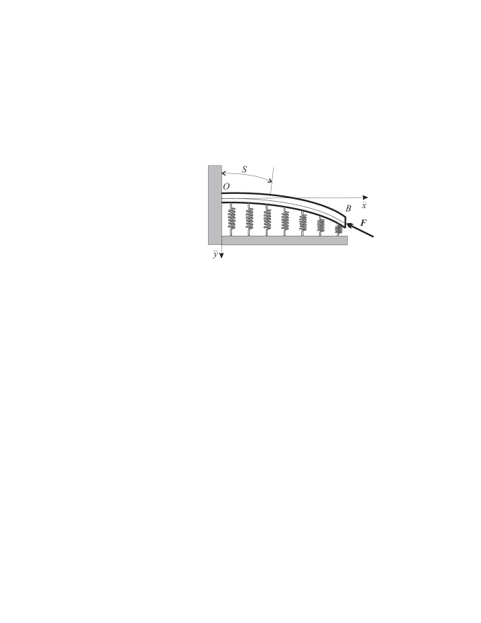
Figure 1: Coordinate system and load configuration.

System of equations describing the lateral motion in $\bar{x}-\bar{y}$ plane for Beck’s column placed on Winkler foundation consists of: equations of motion

$$\frac{\partial}{\partial S}H\left(S,t\right)=\rho\frac{\partial^{2}}{\partial t^{2}}x\left(S,t\right),\;\;\;\;\frac{\partial}{\partial S}V\left(S,t\right)+q_{y}\left(S,t\right)=\rho\frac{\partial^{2}}{\partial t^{2}}y\left(S,t\right),$$ (1)

$$\frac{\partial}{\partial S}M\left(S,t\right)+V\left(S,t\right)\cos\left(\theta\left(S,t\right)\right)-H\left(S,t\right)\sin\left(\theta\left(S,t\right)\right)=0,$$ (2)

geometrical relations

$$\frac{\partial}{\partial S}x\left(S,t\right)=\cos\left(\theta\left(S,t\right)\right),\;\;\;\;\frac{\partial}{\partial S}y\left(S,t\right)=\sin\left(\theta\left(S,t\right)\right),$$ (3)

and constitutive equations:

$$M\left(S,t\right)=EI\frac{\partial}{\partial S}\theta\left(S,t\right),\;\;\;\;q_{y}\left(S,t\right)=-ky\left(S,t\right),$$ (4)

for moment-curvature relation (Bernoulli-Euler) and foundation-rod interaction (Winkler) respectively. The boundary conditions for the system (1) - (4) are

$$x\left(0,t\right)=0,\;\;y\left(0,t\right)=0,\;\;\theta\left(0,t\right)=0,$$

$$H\left(L,t\right)=-F\cos\theta\left(L,t\right),\;\;V\left(L,t\right)=-F\sin\theta\left(L,t\right),\;\;M\left(L,t\right)=0.$$ (5)

In (1) - (4) time is denoted by $t>0,$ the arc-length of rod’s axis is denoted by $S\in\left[0,L\right]$, where $L$ is the length of the rod, $x$ and $y$ denote the coordinates of an arbitrary point on rod’s axis in the deformed state and $\theta$ is the angle between rod’s axis in deformed and undeformed state. Projections of the contact forces on $\bar{x}$ and $\bar{y}$ axes are denoted by $H$ and $V$ respectively, $M$ is the bending moment, $q_{y}$ denotes the distributed forces per unit length describing foundation-rod interaction and $F$ is the intensity of the follower force. Line density, modulus of elasticity, second moment of inertia of the rod and the stiffness of foundation are denoted by $\rho,$ $E,$ $I$ and $k$ respectively. Note that (3) implies that the column axis is inextensible.

The problem of lateral motion of Beck’s column will be treated for the non-local and viscoelastic constitutive moment-curvature equations as opposed to the classical Bernoulli-Euler one. For the case when the material of the rod is modelled by non-local theory of Eringen type, see [14, 15, 25], the constitutive equation for bending moment reads

$$M\left(S,t\right)-l^{2}\frac{\partial^{2}}{\partial S^{2}}M\left(S,t\right)=EI\frac{\partial}{\partial S}\theta\left(S,t\right),$$ (6)

where $l$ is the (constant) length scale parameter. Constitutive equation (6) is often used when modelling materials with size dependent properties as in nano-rod theory. Examples include buckling/post-buckling, vibration and rotation analysis as in [8, 12, 30, 31, 33], [1, 21, 22, 32] and [26], respectively. Optimization of such rods have also been studied in [3, 4, 16].

The constitutive equation

$$M\left(S,t\right)=EI\left(1+a\,{}_{0}\mathrm{D}_{t}^{\alpha}\right)\frac{\partial}{\partial S}\theta\left(S,t\right),$$ (7)

relates to the viscoelastic rod of the fractional Kelvin-Voigt type. In (7), ${}_{0}\mathrm{D}_{t}^{\alpha}$ is the operator of the Riemann-Liouville fractional derivative of order $\alpha\in\left(0,1\right)$ given in the form as

$${}_{0}\mathrm{D}_{t}^{\alpha}f\left(t\right)=\frac{1}{\Gamma(1-\alpha)}\frac{\mathrm{d}}{\mathrm{d}t}\int_{0}^{t}\frac{f(\tau)}{\left(t-\tau\right)^{\alpha}}\mathrm{d}\tau,$$

see [18], where $\Gamma$ is the Euler gamma function and $a$ is the (constant) model parameter. A number of problems treating lateral vibrations of viscoelastic rods of fractional type are reviewed in [6].

The trivial solution to system (1) - (5) corresponding to the case when the rod remains straight is independent of the choice of constitutive equations (6) or (7) and reads

$$x^{0}\left(S,t\right)=S,\;\;y^{0}\left(S,t\right)=0,\;\;\theta^{0}\left(S,t\right)=0,\;\;H^{0}\left(S,t\right)=-F,\;\;V^{0}\left(S,t\right)=0,\;\;M^{0}\left(S,t\right)=0.$$

Assuming $x=x^{0}+\Delta x,\ldots,$ $M=M^{0}+\Delta M$, where $\Delta x,\ldots,\Delta M$ denote the perturbations and upon substitution of perturbed quantities in (1) - (3), (4)₂ and (5), we obtain $\Delta H=0$ and $\Delta x=0$ as well as

$$\frac{\partial}{\partial S}\Delta V\left(S,t\right)=k\Delta y\left(S,t\right)+\rho\frac{\partial^{2}}{\partial t^{2}}\Delta y\left(S,t\right),\;\;\frac{\partial}{\partial S}\Delta M\left(S,t\right)+\Delta V\left(S,t\right)+F\Delta\theta\left(S,t\right)=0,$$ (8)

$$\frac{\partial}{\partial S}\Delta y(S,t)=\Delta\theta\left(S,t\right).$$ (9)

Similarly, constitutive moment-curvature relations (6) and (7) become

$$\Delta M\left(S,t\right)-l^{2}\frac{\partial^{2}}{\partial S^{2}}\Delta M\left(S,t\right)=EI\frac{\partial}{\partial S}\Delta\theta\left(S,t\right),$$ (10)

$$\Delta M\left(S,t\right)=EI\left(1+a\,{}_{0}\mathrm{D}_{t}^{\alpha}\right)\left(\frac{\partial}{\partial S}\Delta\theta\left(S,t\right)\right),$$ (11)

with boundary conditions (5) yielding

$$\Delta y(0,t)=0,\;\;\Delta\theta(0,t)=0,\;\;\Delta V(L,t)=-F\Delta\theta\left(L,t\right),\;\;\Delta M(L,t)=0.$$ (12)

Initial conditions

$$\Delta y\left(S,0\right)=\Delta y_{0}\left(S\right),\;\;\frac{\partial}{\partial t}\Delta y\left(S,0\right)=\Delta y_{1}\left(S\right),$$ (13)

are adjoined to systems (8), (9), (10), (12) and (8), (9), (11), (12).

Introducing the dimensionless quantities

$$\xi=\frac{S}{L},\;\;\bar{t}=t\sqrt{\frac{EI}{\rho L^{4}}},\;\;y=\frac{\Delta y}{L},\;\;y_{0}=\frac{\Delta y_{0}}{L},\;\;y_{1}=\frac{\Delta y_{1}}{L}\sqrt{\frac{\rho L^{4}}{EI}},\;\;\vartheta=\Delta\theta,$$

$$v=\frac{\Delta V\,L^{2}}{EI},\;\;m=\frac{\Delta M\,L}{EI},\;\;\lambda=\frac{FL^{2}}{EI},\;\;\bar{k}=\frac{kL^{4}}{EI},\;\;\kappa=\frac{l}{L},\;\;\bar{a}=a\left(\sqrt{\frac{EI}{\rho L^{4}}}\right)^{\alpha}$$

and upon substitution into (8) - (13), after omitting the bar ($\bar{t}\rightarrow t,$ $\bar{k}\rightarrow k,$ $\bar{a}\rightarrow a$), equations of motion (8) and geometrical relation (9) read

$$\frac{\partial}{\partial\xi}v\left(\xi,t\right)=ky\left(\xi,t\right)+\frac{\partial^{2}}{\partial t^{2}}y\left(\xi,t\right),\;\;\frac{\partial}{\partial\xi}m\left(\xi,t\right)+v\left(\xi,t\right)+\lambda\vartheta\left(\xi,t\right)=0,$$ (14)

$$\frac{\partial}{\partial\xi}y(\xi,t)=\vartheta\left(\xi,t\right),$$ (15)

with non-local (10) and viscoelastic (11) constitutive equations becoming

$$m\left(\xi,t\right)-\kappa^{2}\frac{\partial^{2}}{\partial\xi^{2}}m\left(\xi,t\right)=\frac{\partial}{\partial\xi}\vartheta\left(\xi,t\right),$$ (16)

$$m\left(\xi,t\right)=\left(1+a\,{}_{0}\mathrm{D}_{t}^{\alpha}\right)\left(\frac{\partial}{\partial\xi}\vartheta\left(\xi,t\right)\right),$$ (17)

and boundary (12) and initial conditions (13) transforming to

$$y(0,t)=0,\;\;\vartheta(0,t)=0,\;\;v(1,t)=-\lambda\vartheta\left(1,t\right),\;\;m(1,t)=0,$$ (18)

$$y\left(\xi,0\right)=y_{0}\left(\xi\right),\;\;\frac{\partial}{\partial t}y\left(\xi,0\right)=y_{1}\left(\xi\right).$$ (19)

3 Dynamic stability analysis for non-local rod

The non-local constitutive moment-curvature equation will now be adopted in order to analyse dynamic stability of Beck’s column on Winkler foundation and to determine if the Herrmann-Smith paradox is removed. Adjoining (14), (15), (16) it is derived that

$$\left(1-\kappa^{2}\lambda\right)\frac{\partial^{4}}{\partial\xi^{4}}y\left(\xi,t\right)+\left(\lambda-k\kappa^{2}\right)\frac{\partial^{2}}{\partial\xi^{2}}y\left(\xi,t\right)-\kappa^{2}\frac{\partial^{4}}{\partial\xi^{2}\partial t^{2}}y\left(\xi,t\right)+\frac{\partial^{2}}{\partial t^{2}}y\left(\xi,t\right)+ky\left(\xi,t\right)=0,$$ (20)

subject to boundary (18) and initial (19) conditions

$$y(0,t)=0,\;\;\frac{\partial}{\partial\xi}y(0,t)=0,$$ (21)

$$\left(1-\kappa^{2}\lambda\right)\frac{\partial^{2}}{\partial\xi^{2}}y\left(1,t\right)-\kappa^{2}\frac{\partial^{2}}{\partial t^{2}}y\left(1,t\right)-k\kappa^{2}y\left(1,t\right)=0,$$ (22)

$$\left(1-\kappa^{2}\lambda\right)\frac{\partial^{3}}{\partial\xi^{3}}y\left(1,t\right)-\kappa^{2}\frac{\partial^{3}}{\partial\xi\partial t^{2}}y\left(1,t\right)-k\kappa^{2}\frac{\partial}{\partial\xi}y\left(1,t\right)=0,$$ (23)

$$y\left(\xi,0\right)=y_{0}\left(\xi\right),\;\;\frac{\partial}{\partial t}y\left(\xi,0\right)=y_{1}\left(\xi\right).$$

Assuming variables can be separated in the form of

$$y\left(\xi,t\right)=U\left(\xi\right)V\left(t\right)$$

equation (20) becomes

$$\left(1-\kappa^{2}\lambda\right)\frac{U^{\prime\prime\prime\prime}\left(\xi\right)}{U\left(\xi\right)}+\left(\lambda-k\kappa^{2}\right)\frac{U^{\prime\prime}\left(\xi\right)}{U\left(\xi\right)}-\kappa^{2}\frac{U^{\prime\prime}\left(\xi\right)}{U\left(\xi\right)}\frac{\ddot{V}(t)}{V(t)}+\frac{\ddot{V}(t)}{V(t)}+k=0,$$ (24)

with boundary conditions (21) - (23)

$$U(0)=0,\;\;U^{\prime}(0)=0,$$ (25)

$$\left(1-\kappa^{2}\lambda\right)\frac{U^{\prime\prime}\left(1\right)}{U\left(1\right)}-\kappa^{2}\frac{\ddot{V}(t)}{V(t)}-k\kappa^{2}=0,$$ (26)

$$\left(1-\kappa^{2}\lambda\right)\frac{U^{\prime\prime\prime}\left(1\right)}{U\left(1\right)}-\kappa^{2}\frac{U^{\prime}\left(1\right)}{U\left(1\right)}\frac{\ddot{V}(t)}{V(t)}-k\kappa^{2}\frac{U^{\prime}\left(1\right)}{U\left(1\right)}=0,$$ (27)

where $\left(\cdot\right)^{\prime}=\frac{\mathrm{d}}{\mathrm{d}\xi}\left(\cdot\right)$ and $\left(\cdot\right)^{\cdot}=\frac{\mathrm{d}}{\mathrm{d}t}\left(\cdot\right).$ Introducing new parameter $\Omega$ so that

$$\ddot{V}(t)+\Omega^{2}V(t)=0,$$

equation (24) and boundary conditions (25) - (27) thus become

$$U^{\prime\prime\prime\prime}\left(\xi\right)+r_{1}U^{\prime\prime}\left(\xi\right)-r_{2}U\left(\xi\right)=0,$$ (28)

$$U(0)=0,\;\;U^{\prime}(0)=0,$$ (29)

$$U^{\prime\prime}\left(1\right)+\kappa^{2}r_{2}U\left(1\right)=0,\;\;U^{\prime\prime\prime}\left(1\right)+\kappa^{2}r_{2}U^{\prime}\left(1\right)=0,$$ (30)

where

$$r_{1}=\frac{\lambda+\kappa^{2}\left(\Omega^{2}-k\right)}{1-\kappa^{2}\lambda},\;\;r_{2}=\frac{\Omega^{2}-k}{1-\kappa^{2}\lambda}.$$ (31)

It is assumed that $1-\kappa^{2}\lambda>0$ and $\Omega^{2}-k>0$ leading to $r_{2}>0$.

The general solution to equation (28) is

$$U\left(\xi\right)=C_{1}\cosh\left(p_{1}\xi\right)+C_{2}\sinh\left(p_{1}\xi\right)+C_{3}\cos\left(p_{2}\xi\right)+C_{4}\sin\left(p_{2}\xi\right),$$

with

$$p_{1}=\sqrt{\frac{-r_{1}+\sqrt{r_{1}^{2}+4r_{2}}}{2}},\;\;p_{2}=\sqrt{\frac{r_{1}+\sqrt{r_{1}^{2}+4r_{2}}}{2}}.$$ (32)

Unknown constants $C_{1},...,C_{4}$ should be obtained using boundary conditions (29) and (30). For the existence of non-trivial solution of the homogeneous system with respect to constants, it is required that

$$\sqrt{\text{$r_{2}$}}\left(\text{$r_{1}^{2}$}+2\text{$r_{2}$}+2\left(\kappa^{2}\text{$r_{2}$}\right)^{2}-2\kappa^{2}\text{$r_{1}r_{2}$}\right)$$

$$\qquad\qquad+\left(\text{$r_{2}$}+\kappa^{2}\text{$r_{1}r_{2}$}-\left(\kappa^{2}\text{$r_{2}$}\right)^{2}\right)\left(2\sqrt{\text{$r_{2}$}}\cosh\text{$p_{1}$}\cos\text{$p_{2}$}+\text{$r_{1}$}\sinh\text{$p_{1}$}\sin\text{$p_{2}$}\right)=0.$$ (33)

For the case when $\kappa=0$, relations (31), (32) and (33) reduce to

$$r_{1}=\lambda,\;\;r_{2}=\Omega^{2}-k,\;\;p_{1}=\sqrt{\frac{-\lambda+\sqrt{\lambda^{2}+4\left(\Omega^{2}-k\right)}}{2}},\;\;p_{2}=\sqrt{\frac{\lambda+\sqrt{\lambda^{2}+4\left(\Omega^{2}-k\right)}}{2}},$$

$$\lambda^{2}+2\left(\Omega^{2}-k\right)\left(1+\cosh\text{$p_{1}$}\cos\text{$p_{2}$}\right)+\lambda\sqrt{\Omega^{2}-k}\sinh\text{$p_{1}$}\sin\text{$p_{2}$}=0,$$

giving the relations corresponding to Beck’s column on Winkler foundation as shown in [19] and to classical Beck’s column if additionally $k=0$, see [2].

Equation (33) will be numerically solved in order to determine the effect of non-locality parameter on dynamic stability boundary and to determine if the Herrmann-Smith paradox is removed. This can be mathematically stated as follows: For a given non-locality parameter $\kappa$ and foundation stiffness $k$, determine load intensity $\lambda_{cr}$ and frequency $\Omega_{cr}$ so that the first root of equation (33) has multiplicity two. Numerical procedure of obtaining $\lambda_{cr}$ and $\Omega_{cr}$ was performed for equation (33) using various values of $\kappa$ and $k$. The results are summarised in Table 1.

	$k=0$		$k=5$	$k=10$
$\kappa$	$\lambda_{cr}$	$\Omega_{cr}$	$\Omega_{cr}$	$\Omega_{cr}$
$0$	$20.05095$	$11.01$	$11.24$	$11.46$
$0.1$	$16.79301$	$9.32$
$0.2$	$11.24116$	$6.35$	$6.73$	$7.09$
$0.3$	$7.22022$	$4.13$
$0.4$	$4.80283$	$2.77$	$3.56$	$4.20$
$0.5$	$3.35534$	$1.94$
$0.6$	$2.45147$	$1.42$	$2.65$	$3.47$

Table 1: Critical load intensities $\lambda_{cr}$ and frequencies $\Omega_{cr}$ for different values of non-locality parameter $\kappa$ and foundation stiffness $k$.

For the case when Bernoulli-Euler moment-curvature relation is assumed ($\kappa$ and $k$ equal zero), the critical load $\lambda_{cr}=20.05095$ and critical frequency $\Omega_{cr}=11.01$ corresponding to classical Beck’s column are reobtained, see [2]. This critical load remains unchanged when foundations of varying stiffness are introduced thus recovering the Herrmann-Smith paradox. The results also show that the critical frequency increased with increasing foundation stiffness, which was obtained in [27]. By introducing non-local constitutive equation, the critical load and frequency decrease with the increase of non-locality parameter, as depicted in Figure 2.

Figure 2: Dependence of critical load $\lambda_{cr}$ and frequency $\Omega_{cr}$ on non-locality parameter $\kappa$.

This effect of non-locality parameter on stability boundary was also shown to hold true for static problems of various conservative loading configurations and boundary conditions in [5, 12, 33]. Here it is shown that reduction in critical load also occurs for non-conservative problems when non-local constitutive equation is adopted. As with the Bernoulli-Euler Beck’s column on Winkler foundation, there was no change in critical force for non zero values of foundation stiffness when adopting non-local model. For a fixed value of non-locality parameter, the effect of increasing the foundation stiffness on critical frequency was the same as for Bernoulli-Euler rod. Thus the Herrmann-Smith paradox remains.

4 Dynamic stability analysis for fractional viscoelastic rod

The Herrmann-Smith and Ziegler paradoxes are now examined by determining stability boundaries for Beck’s column described using viscoelastic constitutive equation of fractional Kelvin-Voigt type. Combining (14), (15), (17) it is obtained that

$$\left(1+a\,{}_{0}\mathrm{D}_{t}^{\alpha}\right)\frac{\partial^{4}}{\partial\xi^{4}}y\left(\xi,t\right)+\lambda\frac{\partial^{2}}{\partial\xi^{2}}y\left(\xi,t\right)+\frac{\partial^{2}}{\partial t^{2}}y\left(\xi,t\right)+ky\left(\xi,t\right)=0,$$ (34)

subject to boundary (18) and initial (19) conditions

$$y(0,t)=0,\;\;\frac{\partial}{\partial\xi}y(0,t)=0,$$ (35)

$$\left(1+a\,{}_{0}\mathrm{D}_{t}^{\alpha}\right)\frac{\partial^{2}}{\partial\xi^{2}}y\left(1,t\right)=0,\;\;\left(1+a\,{}_{0}\mathrm{D}_{t}^{\alpha}\right)\frac{\partial^{3}}{\partial\xi^{3}}y\left(1,t\right)=0,$$ (36)

$$y\left(\xi,0\right)=y_{0}\left(\xi\right),\;\;\frac{\partial}{\partial t}y\left(\xi,0\right)=y_{1}\left(\xi\right).$$ (37)

Note that equation (34) reduces to the corresponding one for elastic model when $a\rightarrow 0$ or $\alpha\rightarrow 0$. Contrary to the approach used in Section 3, the Laplace transform method will be implemented to analyse dynamic stability. Applying the Laplace transform to (34) - (36) results in

$$\left(1+as^{\alpha}\right)\frac{\partial^{4}}{\partial\xi^{4}}Y\left(\xi,s\right)+\lambda\frac{\partial^{2}}{\partial\xi^{2}}Y\left(\xi,s\right)+(s^{2}+k)Y\left(\xi,s\right)=sy_{0}\left(\xi\right)+y_{1}\left(\xi\right),$$ (38)

$$Y(0,s)=0,\;\;\frac{\partial}{\partial\xi}Y(0,s)=0,$$ (39)

$$\left(1+as^{\alpha}\right)\frac{\partial^{2}}{\partial\xi^{2}}Y\left(1,s\right)=0,\;\;\left(1+as^{\alpha}\right)\frac{\partial^{3}}{\partial\xi^{3}}Y\left(1,s\right)=0,$$ (40)

where the Laplace transform of a function $f$ is defined by

$$F\left(s\right)=\mathcal{L}\left[f\left(t\right)\right]\left(s\right)=\int_{0}^{\infty}f\left(t\right)\mathrm{e}^{-st}\mathrm{d}t,$$

and the Laplace transform of a Riemann-Liouville fractional derivative is

$$\mathcal{L}\left[{}_{0}\mathrm{D}_{t}^{\alpha}f(t)\right]\left(s\right)=s^{\alpha}F(s)-\left[\frac{1}{\Gamma(1-\alpha)}\int_{0}^{t}\frac{f(\tau)}{(t-\tau)^{\alpha}}d\tau\right]_{t=0}=s^{\alpha}F(s),$$

provided that $f$ is an exponentially bounded function, see [18]. Equation (38) reduces to

$$\frac{\partial^{4}}{\partial\xi^{4}}Y\left(\xi,s\right)+r_{1}(s)\frac{\partial^{2}}{\partial\xi^{2}}Y\left(\xi,s\right)+r_{2}(s)Y\left(\xi,s\right)=F(\xi,s),$$ (41)

with

$$r_{1}(s)=\frac{\lambda}{1+as^{\alpha}},\;\;r_{2}(s)=\frac{s^{2}+k}{1+as^{\alpha}},\;\;F(\xi,s)=\frac{sy_{0}\left(\xi\right)+y_{1}\left(\xi\right)}{1+as^{\alpha}}.$$ (42)

The general solution to equation (41) is

$$Y(\xi,s)=Y_{H}(\xi,s)+Y_{P}(\xi,s),$$ (43)

where

$$Y_{H}(\xi,s)=C_{1}(s)\cosh\left(p_{1}(s)\xi\right)+C_{2}(s)\sinh\left(p_{1}(s)\xi\right)+C_{3}(s)\cos\left(p_{2}(s)\xi\right)+C_{4}(s)\sin\left(p_{2}(s)\xi\right),$$ (44)

is the solution of homogeneous equation, with

$$p_{1}=\sqrt{\frac{-r_{1}+\sqrt{r_{1}^{2}-4r_{2}}}{2}},\;\;p_{2}=\sqrt{\frac{r_{1}+\sqrt{r_{1}^{2}-4r_{2}}}{2}},$$

and $Y_{P}$ is the particular solution of equation (41).

The general solution (43) takes the form

$$Y(\xi,s) = \frac{1}{D(s)}\left(D_{C_{1}}(s)\cosh\left(p_{1}(s)\xi\right)+D_{C_{2}}(s)\sinh\left(p_{1}(s)\xi\right)\right.$$ (45)

$$+\left.D_{C_{3}}(s)\cos\left(p_{2}(s)\xi\right)+D_{C_{4}}(s)\sin\left(p_{2}(s)\xi\right)\right)+Y_{P}(\xi,s),$$

with the fact that $C_{1}=\frac{D_{C_{1}}}{D},...,C_{4}=\frac{D_{C_{4}}}{D},$ where $D,D_{C_{1}},...,D_{C_{4}}$ are the determinants corresponding to system

$$Y(0,s)=0 = C_{1}(s)+C_{3}(s)+Y_{P}(0,s),$$

$$\frac{\partial}{\partial\xi}Y(0,s)=0 = C_{2}(s)p_{1}(s)+C_{4}(s)p_{2}(s)+\frac{\partial}{\partial\xi}Y_{P}(0,s),$$

$$\frac{\partial^{2}}{\partial\xi^{2}}Y(1,s)=0 = C_{1}(s)p_{1}^{2}(s)\cosh\left(p_{1}(s)\right)+C_{2}(s)p_{1}^{2}(s)\sinh\left(p_{1}(s)\right)$$

$$-C_{3}(s)p_{2}^{2}(s)\cos(p_{2}(s))-C_{4}(s)p_{2}^{2}(s)\sin\left(p_{2}(s)\right)+\frac{\partial^{2}}{\partial\xi^{2}}Y_{P}(1,s),$$

$$\frac{\partial^{3}}{\partial\xi^{3}}Y(1,s)=0 = C_{1}(s)p_{1}^{3}(s)\sinh\left(p_{1}(s)\right)+C_{2}(s)p_{1}^{3}(s)\cosh\left(p_{1}(s)\right)$$

$$+C_{3}(s)p_{2}^{3}(s)\sin(p_{2}(s))-C_{4}(s)p_{2}^{3}(s)\cos\left(p_{2}(s)\right)+\frac{\partial^{3}}{\partial\xi^{3}}Y_{P}(1,s).$$

This system is obtained by substitution of boundary conditions (39) and (40) in (43) and (44). The particular solution $Y_{P}$ is dependent on initial conditions, see (41) and (42). Following the standard procedure for stability analysis, the stability boundaries will be determined regardless of the choice of initial conditions. Thus the determinant of system

$$D\left(s\right)=\text{$r_{1}^{2}\left(s\right)$}-2\text{$r_{2}\left(s\right)$}\left(1+\cosh\left(\text{$p_{1}\left(s\right)$}\right)\cos\left(\text{$p_{2}\left(s\right)$}\right)\right)+\text{$r_{1}\left(s\right)$}\sqrt{-\text{$r_{2}\left(s\right)$}}\text{$\sinh$}\left(\text{$p_{1}\left(s\right)$}\right)\sin\left(\text{$p_{2}\left(s\right)$}\right)$$ (46)

will be the focus of stability analysis. The position of zeroes of (46) will determine the dynamic behaviour of the rod. If zeroes are positioned in the left complex half plane or on the imaginary axis, the rod will be stable with decreasing or constant amplitude of oscillation respectively. Loss of stability occurs when zero has positive real part resulting in vibrations of increasing amplitude. Thus the critical force is determined as the force corresponding to zero of (46) having real part equal to zero. The corresponding value of imaginary part represents the critical frequency. For similar method of stability boundary analysis, we refer to [28, 29]. The critical force $\lambda_{cr}$ and frequency $\Omega_{cr}$ will be numerically determined using (46) for various values of order of fractional differentiation $\alpha$ and foundation stiffness $k$.

Table 2 shows the values of critical force $\lambda_{cr}$ and frequency $\Omega_{cr}$ for viscoelastic Beck’s column with fixed value of model parameter $a=0.4$ when order of differentiation $\alpha$ is varied.

$\alpha$	$\lambda_{cr}$	$\Omega_{cr}$
$0$	$28.0713$	$13.0431$
$0.01$	$15.4000$	$6.4055$
$0.1$	$16.1912$	$6.5619$
$0.3$	$18.5037$	$6.9258$
$0.5$	$22.2605$	$7.2553$
$0.7$	$29.2249$	$7.4182$
$0.9$	$42.2860$	$7.1619$
$1$	$51.4069$	$6.7645$

Table 2: Critical load intensities $\lambda_{cr}$ and frequencies $\Omega_{cr}$ for different values of order of fractional differentiation $\alpha$, with foundation stiffness $k=0,$ and model parameter $a=0.4$.

For the case when $\alpha$ is zero, the dimensionless fractional Kelvin-Voigt model (17) reduces to Bernoulli-Euler equation $m=(1+a)\frac{\partial}{\partial\xi}\vartheta$. The critical force $\lambda_{cr}=28.0713$ corresponding to this case reduces to the critical force $\lambda_{cr}=20.0510$ for classical Beck’s column when divided by $1+a$. By introducing small values of $\alpha$, the model becomes of fractional Kelvin-Voigt type and there is a reduction in critical force. This result is the Ziegler paradox. In [11], it was found that for extremely small values of viscoelastic model parameter, thus approaching elastic model, the critical force is less then in the elastic case (model parameter is zero). The same result was achieved in our analysis however the order of fractional differentiation approached zero, reducing the fractional derivative of a function to a function itself, thus obtaining the elastic model, as opposed to the case when the elastic model was recovered by introduction of small model parameter.

The critical force increases with the order of fractional differentiation, see Figure 3, as is to be expected due to greater dissipation.

Figure 3: Dependence of critical load $\lambda_{cr}$ on order of fractional differentiation $\alpha$ with dot representing critical load for elastic case.

A decrease in the value of critical frequency occurs when small order of differentiation is introduced, similarly to the behaviour of critical force. The critical frequency however shows non-monotonic dependence on the order of differentiation with maximum value occurring in the range of $\alpha\in(0.5,0.9)$ as shown in Figure 4.

Figure 4: Dependence of critical frequency $\Omega_{cr}$ on order of fractional differentiation $\alpha$ with dot representing critical frequency for elastic case.

The effect of foundation stiffness on critical load and frequency is analysed for given values of order of differentiation $\alpha=0.3$ and $\alpha=0.9$ with model parameter $a=0.4$. The results of this analysis are shown in Table 3.

	$\alpha=0.3$		$\alpha=0.9$
$k$	$\lambda_{cr}$	$\Omega_{cr}$	$\lambda_{cr}$	$\Omega_{cr}$
$0$	$18.5037$	$6.9258$	$42.2860$	$7.1619$
$5$	$18.6295$	$7.2985$	$44.6815$	$7.6008$
$10$	$18.7446$	$7.6514$	$46.9197$	$8.0094$
$20$	$18.9495$	$8.3086$	$51.0257$	$8.7559$
$40$	$19.2880$	$9.4785$	$58.1810$	$10.0508$

Table 3: Critical load intensities $\lambda_{cr}$ and frequencies $\Omega_{cr}$ for different values of foundation stiffness $k$, and model parameter $a=0.4$.

The presence of foundation is shown to influence the value of critical load causing it to increase as the foundation stiffness does. The Herrmann-Smith paradox is thus resolved when adopting fractional Kelvin-Voigt moment-curvature constitutive equation. The critical frequency also increases as in the case of classical Beck’s column on elastic foundation.

5 Conclusion

The stability boundaries for Beck’s column positioned on elastic foundation have been analysed when adopting non-local and viscoelastic moment-curvature constitutive equations for the column with the aim of removing the Herrmann-Smith paradox. For the case of nano-rod of Eringen non-local type, the separation of variables technique was adopted in order to determine critical load causing dynamic instability, whereas the Laplace transform method was utilised for the same analysis of viscoelastic rod of fractional Kelvin-Voigt type.

The introduction of non-locality was found to reduce the load causing flutter which is generally true for nano-rods. The Herrmann-Smith paradox remained as the critical load is independent of foundation properties whilst the critical frequency increased when the foundation stiffness did. The removal of the Herrmann-Smith paradox was achieved by adoption of fractional Kelvin-Voigt moment-curvature relation describing the column. In this case, the critical load increased with higher orders of fractional differentiation which is to be expected due to increased dissipation. However for orders of fractional differentiation close to zero, the load causing dynamic instability was less then for the elastic case despite the fact that the viscoelastic model approached the elastic one. Therefore the Ziegler paradox of destabilization is recovered.

References

• [1] J. Aranda-Ruiz, J. Loya, and J. Fernández-Sáez. Bending vibrations of rotating nonuniform nanocantilevers using the Eringen nonlocal elasticity theory. Composite Structures, 94:2990–3001, 2012.
• [2] T. M. Atanackovic. Stability Theory of Elastic Rods. World Scientific, New Jersay, 1997.
• [3] T. M. Atanackovic, B. N. Novakovic, and Z. Vrcelj. Application of Pontryagin’s principle to bimodal optimization of nano rods. International Journal of Structural Stability and Dynamics, 12:1250012, 11 pp, 2012.
• [4] T. M. Atanackovic, B. N. Novakovic, and Z. Vrcelj. Shape optimization against buckling of micro- and nano-rods. Archive of Applied Mechanics, 82:1303–1311, 2012.
• [5] T. M. Atanackovic, B. N. Novakovic, Z. Vrcelj, and D. Zorica. Rotating nanorod with clamped ends. International Journal of Structural Stability and Dynamics, DOI: 10.1142/S0219455414500503:1450050, 2014.
• [6] T. M. Atanackovic, S. Pilipovic, B. Stankovic, and D. Zorica. Fractional Calculus with Applications in Mechanics: Vibrations and Diffusion Processes. Wiley-ISTE, London, 2014.
• [7] T. M. Atanackovic and B. Stankovic. On a system of differential equations with fractional derivatives arising in rod theory. Journal of Physics A: Mathematical and General, 37:1241–1250, 2004.
• [8] T. M. Atanackovic and D. Zorica. Stability of the rotating compressed nano-rod. Zeitschrift für Angewandte Mathematik und Mechanik, 94:499–504, 2014.
• [9] M. Beck. Die Knicklast des einseitig eingespannten, tangential gedrückten Stabes. Zeitschrift für angewandte Mathematik und Physik, 3:225–228, 1952.
• [10] M. Becker, W. Hauger, and W. Winzen. Influence of internal and external damping on the stability of Beck’s column on an elastic foundation. Journal of Sound and Vibration, 54:468–472, 1977.
• [11] V. V. Bolotin and N. I. Zhinzher. Effects of damping on stability of elastic systems subjected to nonconservative forces. International Journal of Solids and Structures, 5:965–989, 1969.
• [12] N. Challamel and C. M. Wang. On lateral-torsional buckling of non-local beams. Advances in Applied Mathematics and Mechanics, 2:389–398, 2010.
• [13] I. Elishakoff. Controversy associated with the so-called ”follower forces”: critical overview. Applied Mechanics Reviews, 58:117–142, 2005.
• [14] I. Elishakoff, D. Pentaras, K. Dujat, C. Versaci, G. Muscolino, J. Storch, S. Bucas, N. Challamel, T. Natsuki, Y. Y. Zhang, C. M. Wang, and G. Ghyselinck. Carbon Nanotubes And Nanosensors: Vibrations, Buckling And Ballistic Impact. ISTE and John Wiley & Sons, London, New York, 2012.
• [15] A. C. Eringen. Nonlocal Continuum Field Theories. Springer Verlag, New York, 2002.
• [16] V. B. Glavardanov, D. T. Spasic, and T. M. Atanackovic. Stability and optimal shape of Pflüger micro/nano beam. International Journal of Solids and Structures, 49:2559–2567, 2012.
• [17] J. T. Katsikadelis and G. C. Tsiatas. Non-linear dynamic stability of damped Beck’s column with variable cross-section. International Journal of Non-Linear Mechanics, 42:164–171, 2007.
• [18] A. A. Kilbas, H. M. Srivastava, and J. J. Trujillo. Theory and Applications of Fractional Differential Equations. Elsevier B.V., Amsterdam, 2006.
• [19] O. N. Kirillov and A. P. Seyranian. Solution to the Herrmann-Smith problem. Doklady Physics, 47:767–771, 2002.
• [20] M. A. Langthjem and Y. Sugiyama. Dynamic stability of columns subjected to follower loads: a survey. Journal of Sound and Vibration, 238:809–851, 2000.
• [21] Y. Lei, S. Adhikari, and M. I. Friswell. Vibration of nonlocal Kelvin-Voigt viscoelastic damped Timoshenko beams. International Journal of Engineering Science, 66-67:1–13, 2013.
• [22] C. Li, C. W. Lim, J. L. Yu, and Q. C. Zeng. Analytical solutions for vibration of simply supported nonlocal nanobeams with an axial force. International Journal of Structural Stability and Dynamics, 11:257–271, 2011.
• [23] M. R. Morgan and S. C. Sinha. Influence of a viscoelastic foundation on the stability of Beck’s column: an exact analysis. Journal of Sound and Vibration, 91:85–101, 1983.
• [24] J. G. Panovko and I. I. Gubanova. Stability and oscillation of elastic systems: modern concepts, paradoxes and errors (in Russian). Nauka, Moscow, 1987.
• [25] J. N. Reddy. Nonlocal theories for bending, buckling and vibration of beams. International Journal of Engineering Science, 45:288–307, 2007.
• [26] J. N. Reddy and S. El-Borgi. Eringen’s nonlocal theories of beams accounting for moderate rotations. International Journal of Engineering Science, 82:159–177, 2014.
• [27] T. E. Smith and G. Herrmann. Stability of a beam on an elastic foundation subjected to a follower force. Journal of Applied Mechanics. Transactions ASME, 39:628–629, 1972.
• [28] B. Stankovic and T. M. Atanackovic. On a model of a viscoelastic rod. Fractional Calculus and Applied Analysis, 4:501–522, 2001.
• [29] B. Stankovic and T. M. Atanackovic. On a viscoelastic rod with constitutive equation containing fractional derivative of two different orders. Mathematics and Mechanics of Solids, 9:629–656, 2004.
• [30] H-T. Thai. A nonlocal beam theory for bending, buckling, and vibration of nanobeams. International Journal of Engineering Science, 52:56–64, 2012.
• [31] C. M. Wang, Y. Xiang, and S. Kitipornchai. Postbuckling of micro and nano rods/tubes based on nonlocal beam theory. International Journal of Applied Mechanics, 1:259–266, 2009.
• [32] C. M. Wang, Y. Y. Zhang, and X. Q. He. Vibration of nonlocal Timoshenko beams. Nanotechnology, 18:105401–105409, 2007.
• [33] C. M. Wang, Y. Y. Zhang, S. S. Ramesh, and S. Kitipornchai. Buckling analysis of micro- and nano-rods/tubes based on nonlocal Timoshenko beam theory. Journal of Physics D: Applied Physics, 39:3904–3909, 2006.
• [34] H. Ziegler. Die Stabilia tskriterien der Elastomechanik. Ingenieur-Archiv, 20:49–56, 1952.