• NMLS-G: the nonmonotone line search of Grippo et al. GriLL1;

• NMLS-H: the nonmonotone line search of Zhang & Hager ZhaH;

• NMLS-N: the nonmonotone line search of Amini et al. AmiAN;

• NMLS-M: the nonmonotone line search of Ahookhosh et al. AhoAB1;

• NMLS-1: a version of Algorithm 2 using the nonmonotone term (LABEL:e.tk2);

• NMLS-2: a version of Algorithm 2 using the nonmonotone term (LABEL:e.tk1);

All of these codes are written in MATLAB using the same subroutine, and they are tested on 2Hz core i5 processor laptop with 4GB of RAM with double precision format. The initial points are standard ones reported in And and MorGH. All the algorithms use the parameters $\rho=0.5$ and $\sigma=0.01$. For NMLS-N, NMLS-G, NMLS-1 and NMLS-2, we set $N=10$. As discussed in ZhaH, NMLS-H uses $\eta_{k}=0.85$. On the basis of our experiments, we update the parameter $\eta_{k}$ adaptively by

$$\eta_{k}=\left\{\begin{array}[]{ll}\eta_{0}/2\vspace{4mm}&~{}~{}\mathrm{if}~{}k=1;\\ (\eta_{k-1}+\eta_{k-2})/2&~{}~{}\mathrm{if}~{}k\geq 2,\end{array}\right.$$ (19)

for NMLS-N, NMLS-M, NMLS-1 and NMLS-2, where the parameter $\eta_{0}$ will be tuned to get a better performance. In our experiments, the algorithms are stopped whenever the total number of iterates exceeds $\mathsf{maxiter}=50000$ or

$$\|g_{k}\|<\epsilon$$ (20)

holds with the accuracy parameter $\epsilon=10^{-5}$. We further declare an algorithm ”failed” if the maximum number of iterations is reached.

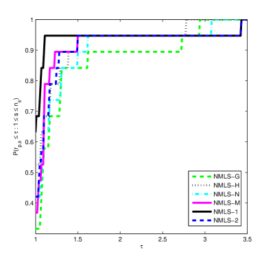
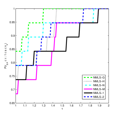
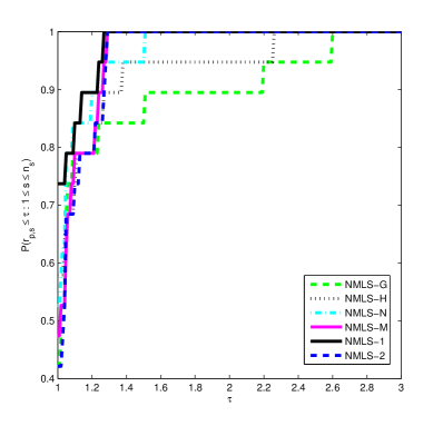
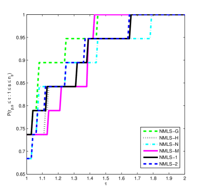
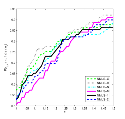
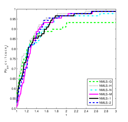
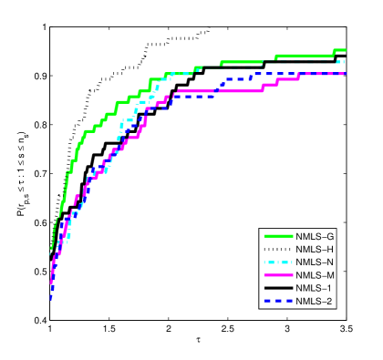
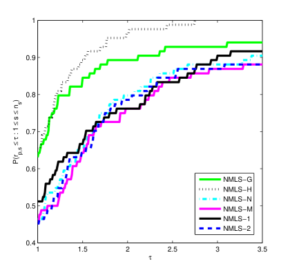
To compare the results appropriately, we use the performance profiles of Dolan & Moré in R7, where the measures of performance are the number of iterations ($N_{i}$), function evaluations ($N_{f}$) and gradient evaluations ($N_{g}$). It is clear that in the considered algorithms the number of iterations and gradient evaluations are the same, so we only consider the performance of gradients. It is believed that computing a gradient is as costly as computing three function values, i.e., we further consider the measure $N_{f}+3N_{g}$. In details, the performance of each code is measured by considering the ratio of its computational outcome versus the best numerical outcome of all codes. This profile offers a tool for comparing the performance of iterative processes in a statistical structure. Let $\mathcal{S}$ be a set of all algorithms and $\mathcal{P}$ be a set of test problems. For each problem $p$ and solver $s$, $t_{p,s}$ is the computational outcome regarding to the performance index, which is used in defining the next performance ratio

$$r_{p,s}=\frac{t_{p,s}}{\min\{t_{p,s}:s\in\mathcal{S}\}}.$$ (21)

If an algorithm $s$ is failed to solve a problem $p$, the procedure sets $r_{p,s}=r_{failed}$, where $r_{failed}$ should be strictly larger than any performance ratio (21). For any factor $\tau$, the overall performance of a algorithm $s$ is given by

$$\rho_{s}(\tau)=\frac{1}{n_{p}}\textrm{size}\{p\in\mathcal{P}:r_{p,s}\leq\tau\}.$$

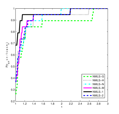
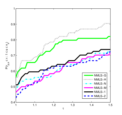
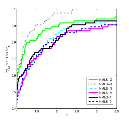
In fact $\rho_{s}(\tau)$ is the probability that a performance ratio $r_{p,s}$ of the algorithm $s\in\mathcal{S}$ is within a factor $\tau\in\mathbf{R}^{n}$ of the best possible ratio. The function $\rho_{s}(\tau)$ is a distribution function for the performance ratio. In particular, $\rho_{s}(1)$ gives the probability that an algorithm $s$ wins over all other considered algorithms, and $\lim_{\tau\rightarrow r_{failed}}\rho_{s}(\tau)$ gives the probability of that algorithm $s$ solve all considered problems. Therefore, this performance profile can be considered as a measure of efficiency among all considered algorithms. In Figures 1-4, the x-axis shows the number $\tau$ while the y-axis inhibits $P(r_{p,s}\leq\tau:1\leq s\leq n_{s})$.

3.1 Experiments with damped Newton and BFGS

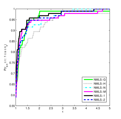
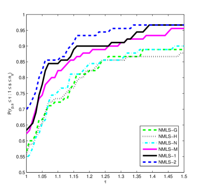
In this section, we report numerical results of solving the problem (LABEL:e.func) by NMLS-G, NMLS-H, NMLS-N, NMLS-M, NMLS-1 and NMLS-2 using damped Newton and BFGS directions and compare their performance. Since both damped Newton and BFGS methods require to solve a linear system of equations in each iteration, it is expected to solve large-scale problems with them. Thus we only consider 18 small-scale test problems from Moré MorGH with their standard initial points. For NMLS-1 and NMLS-2, we use $\eta_{0}=0.75$. The results for damped Newton’s method and the BFGS method are summarized in Tables 1 and 2, respectively.

Table 1 and 2 show that the results are comparable for the considered algorithms, however NMLS-1 and NMLS-2 perform slightly better. To see the results of implementations in details, we illustrate the results with performance profile in Figure 3 with $N_{g}$, $N_{f}$ and $N_{f}+3N_{g}$ as measures of performance. Subfigures (a), (c) and (e) of Figure 3 show the results of damped Newton’s method, while subfigures (b), (d) and (f) of Figure 3 demonstrate the results of the BFGS method.

(a)

(b)

(c)

(d)

(e)

(f)

Figure 3: Performance profiles of all considered algorithms with the performance measures: (a) and (b) for the number of iterations ($N_{i}$) or gradient evaluations ($N_{g}$); (c) and (d) for the number of function evaluations ($N_{f}$); (e) and (f) for the hybrid measure $N_{f}+3N_{g}$.

3.2 Experiments with LBFGS

In the recent decades, the interest for solving optimization problems with large number of variables is remarkably increased thanks to the dramatic emerge of big data in science and technology. This section devotes to an experiment with the considered algorithms with LBFGS which is the limited memory version of the BFGS scheme, and that is much more appropriate for solving large problems, see LiuN; Noc.

The LBFGS scheme calculates a search direction by $d_{k}=-H_{k}g_{k}$, where $H_{k}$ is an approximate of inverse Hessian determined by

$$\begin{split}H_{k+1}&=(V_{k}^{T}\cdots V_{k-m}^{T})H_{0}(V_{k-m}\cdots V_{k})\\ &+\rho_{k-m}(V_{k}^{T}\cdots V_{k-m+1}^{T})s_{k-m}s_{k-m}^{T}(V_{k-m+1}\cdots V_{k})\\ &+\rho_{k-m+1}(V_{k}^{T}\cdots V_{k-m+2}^{T})s_{k-m+1}s_{k-m+1}^{T}(V_{k-m+2}\cdots V_{k})\\ &\vdots\\ &+\rho_{k}s_{k}s_{k}^{T},\end{split}$$

in which $\rho_{k}=1/y_{k}^{T}s_{k}$ and $V_{k}=I-\rho_{k}y_{k}s_{k}^{T}$. The scheme starts from a symmetric positive definite initial matrix $H_{0}$ and sets ${m}={\min}\{k,10\}$. Indeed, it does not need to save the previous approximate matrix, instead it employs only small number of former information to construct the new search direction $d_{k}$. This causes that the method needs much less memory compared with the original BFGS method making it suitable for solving large-scale problems. The LBFGS code is publicly available from Url1, however, we rewrite it in MATLAB.

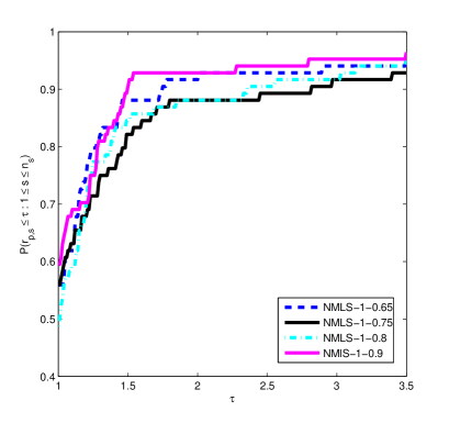
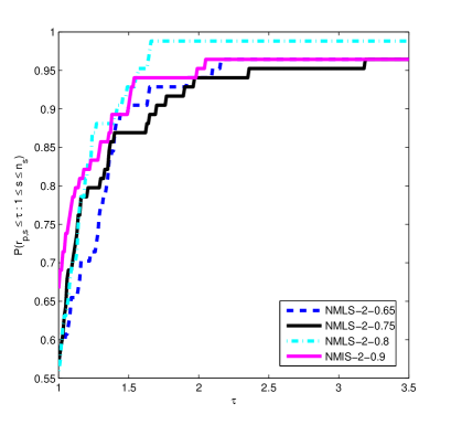
It is believed that nonmonotone algorithms perform better when they employ a stronger nonmonotone term far away from the optimizer and a weaker term close to it. Hence, to get the best performance of the proposed algorithms, we first conduct some test to find a better starting parameter for $\eta_{0}$ in the adaptive process (19). To this end, for both algorithms NMLS-1 and NMLS-2, we consider cases that the algorithms start from $\eta_{0}=0.65$, $\eta_{0}=0.75$, $\eta_{0}=0.85$ and $\eta_{0}=0.95$. The corresponding versions of algorithms NMLS-1 and MNLS-2 are denoted by NMLS-1-0.65, NMLS-1-0.75, NMLS-1-0.85, NMLS-1-0.95, NMLS-2-0.65, NMLS-2-0.75, NMLS-2-0.85 and NMLS-2-0.95, respectively. The results of this test are summarized in Figure 4.

(a)

(b)

(c)

(d)

(e)

(f)

Figure 4: Performance profiles of NMLS-1 and NMLS-2 with the performance measures: (a) and (b) for the number of iterations ($N_{i}$) or gradient evaluations ($N_{g}$); (c) and (d) for the number of function evaluations ($N_{f}$); (e) and (f) for the hybrid measure $N_{f}+3N_{g}$.

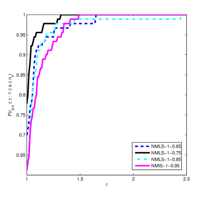
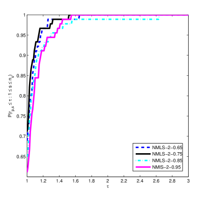
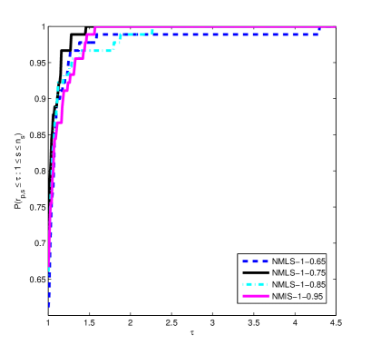
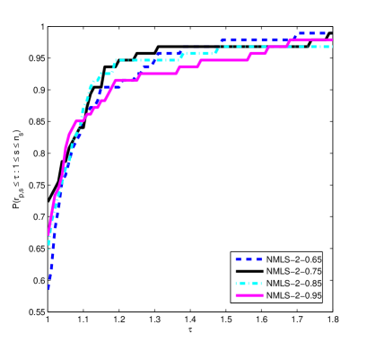
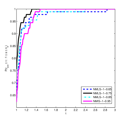
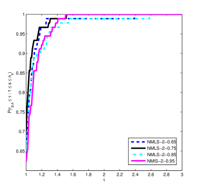
In Figure 4, subfigures (a), (c) and (e) suggest that the results of NMLS-1 with $\eta_{0}=0.75$ are considerably better than those reported for others parameters regarding all of considered measures. In particular, it wins 77%, 73% and 75% score among others for $N_{i}$, $N_{f}$ and $N_{f}+3N_{g}$, respectively. The same results for NMLS-2 in subfigures (b), (d) and (f) of Figure 4 can be observed, where NMLS-2-0.75 respectively wins in 70%, 71% and 70% of the cases for the considered measures. Therefore, we consider $\eta_{0}=0.75$ for our algorithms and for the sake of simplicity denote NMLS-1-0.75 and NMLS-2-0.75 by NMLS-1 and NMLS-2 in the rest of the paper.

(a)

(b)

(c)

(d)

Figure 5: Performance profiles of all considered algorithms measured by: (a) the number of iterations ($N_{i}$) or gradient evaluations ($N_{g}$); (b) the number of function evaluations ($N_{f}$); (c) and (d) the hybrid measure $N_{f}+3N_{g}$.

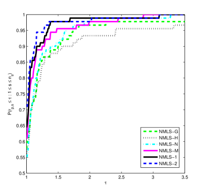
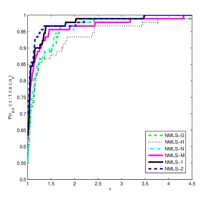
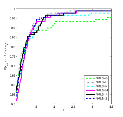
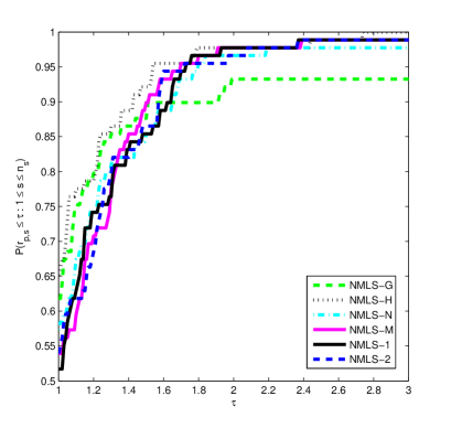
In this point, we test NMLS-G, NMLS-H, NMLS-R, NMLS-M, NMLS-1 and NMLS-2 to solve the problem (LABEL:e.func) by the LBFGS direction. Results of implementation are illustrated in Figure 5. From subfigure (a) of Figure 5, NMLS-2 obtains the most wins by 71%, then NMLS-1 has the next place by 64%. Moreover, NMLS-1 and NMLS-2 solve all problems in about $\tau=3.8$. The subfigure (b) of Figure 5 demonstrates the number of function evaluations suggesting the similar results discussed about the subfigure (a). In Figure 5, subfigures (c) and (d) illustrate the performance profile of the algorithms with the measure $N_{f}+3N_{g}$ by different amount of $\tau$ indicating that NMLS-1 and NMLS-2 win by 63% and 70% score among others, and they also solve the problems in less amount of $\tau$.

3.3 Experiment with Barzilai-Borwein

The Barzilai-Borwein (BB) method for solving the problem (LABEL:e.func) is a gradient-type method proposed by Barzilai & Borwein in BarB, where a step-size along the gradient descent direction $-g_{k}$ is generated using a two-point approximation of the secant equation $B_{k}s_{k-1}=y_{k-1}$ with $s_{k-1}=x_{k-1}-x_{k-2}$ and $y_{k-1}=g_{k-1}-g_{k-2}$. In particular, by imposing $B_{k}=\sigma_{k}I$ and solving the least-squares problem

$$\begin{array}[]{ll}\textrm{minimize}&~{}\|\sigma s_{k-1}-y_{k-1}\|_{2}^{2}\\ \textrm{subject to}&~{}\sigma\in\mathbb{R},\end{array}$$

one can obtain

$$\sigma_{k}^{BB1}=\frac{s_{k-1}^{T}y_{k-1}}{s_{k-1}^{T}s_{k-1}}.$$

Hence the two-point approximated quasi-newton direction is computed by

$$d_{k}=-\left(\sigma_{k}^{BB1}\right)^{-1}g_{k}=-\frac{s_{k-1}^{T}s_{k-1}}{s_{k-1}^{T}y_{k-1}}g_{k}.$$

Since $\sigma_{k}$ in this direction can be unacceptably small or large for non-quadratic objective function, we use the following safeguarded step-size

$$d_{k}^{BB1}=\left\{\begin{array}[]{ll}-\left(\sigma_{k}^{BB1}\right)^{-1}g_{k}&~{}~{}\mathrm{if}~{}10^{-10}\leq\left(\sigma_{k}^{BB1}\right)^{-1}\leq 10^{10},\\ \\ -g_{k}&~{}~{}\mathrm{otherwise.}\end{array}\right.$$ (22)

Similarly, setting $B_{k}^{-1}=\frac{1}{\sigma_{k}}I$ and solving the minimization problem

$$\begin{array}[]{ll}\textrm{minimize}&~{}\|s_{k-1}-\frac{1}{\sigma}y_{k-1}\|_{2}^{2}\\ \textrm{subject to}&~{}\sigma\in\mathbb{R},\end{array}$$

we obtain the step-size

$$\sigma_{k}^{BB2}=\frac{y_{k-1}^{T}s_{k-1}}{y_{k-1}^{T}y_{k-1}}.$$

Considering the safeguard used in (22), we obtain the following search direction

$$d_{k}^{BB2}=\left\{\begin{array}[]{ll}-\left(\sigma_{k}^{BB2}\right)^{-1}g_{k}&~{}~{}\mathrm{if}~{}10^{-10}\leq\left(\sigma_{k}^{BB2}\right)^{-1}\leq 10^{10},\\ \\ -g_{k}&~{}~{}\mathrm{otherwise.}\end{array}\right.$$ (23)

The numerical experiments with the Barzilai-Borwein directions have shown the significant development in efficiency of gradient methods. Being computationally efficient and needing low memory requirement make this scheme interesting to solve large-scale optimization problems. Therefore, it receives much attention during the last two decades and lots of modifications and developments for both unconstrained and constrained optimization have been proposed, for example see AndBM; BirMR1; BirMR2; DaiF; DaiHSZ; DaiYY; HagMZ; JudRRS; LueRGH; Ray and references therein.

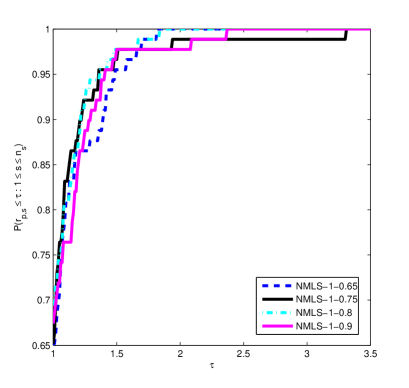
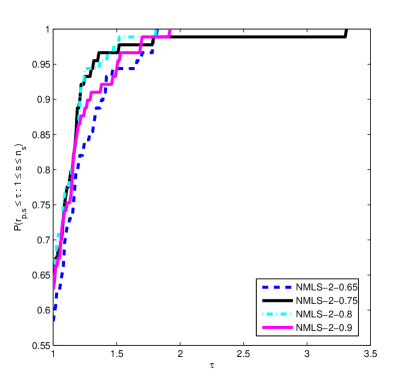
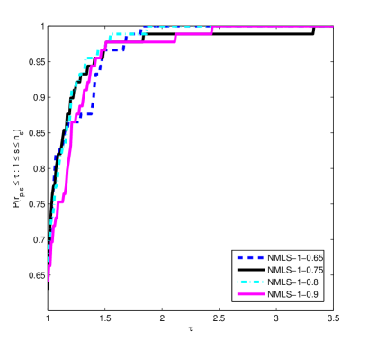
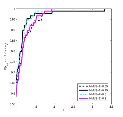
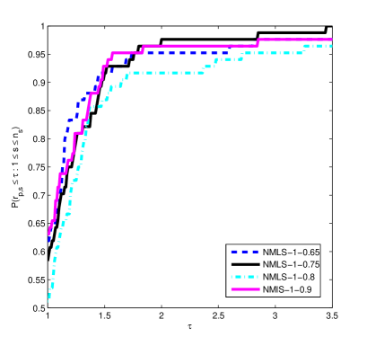
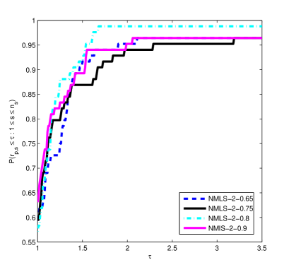
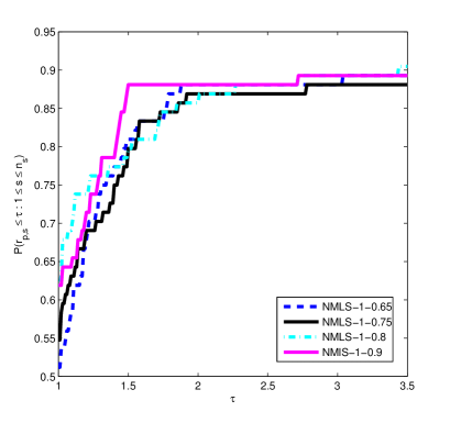
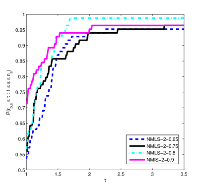
In the rest of this subsection, we consider versions of Algorithm 2 equipped with the nonmonotone terms using the Barzilai-Borwein directions (22) and (23) for solving the problem (LABEL:e.func). We here set $\sigma=10^{-4}$. To find the best possible parameter $\eta_{0}$, we consider $\eta_{0}=0.65$, $\eta_{0}=0.75$, $\eta_{0}=0.80$ and $\eta_{0}=0.90$ and run NMLS-1 and NMLS-2 for both directions (22) and (23). The corresponding results are summarized in Figures 6 and 7, where the first row shows the performance profile for the number of gradients $N_{g}$, the second row shows the performance profile for the number of function evaluations $N_{f}$ and the third row shows the performance profile for $N_{f}+3N_{g}$. From all subfigures of Figures 6 and 7, we conclude that $\eta_{0}=0.80$ and $\eta_{0}=0.90$ produce acceptable results for our algorithms with respect to the directions (22) and (23), i.e., NMLS-1 and NMLS-2 exploit $\eta_{0}=0.80$ and $\eta_{0}=0.90$ for these directions, respectively.

(a)

(b)

(c)

(d)

(e)

(f)

Figure 6: Performance profiles of NMLS-1 and NMLS-2 with the performance measures: (a) and (b) for the number of iterations ($N_{i}$) or gradient evaluations ($N_{g}$); (c) and (d) for the number of function evaluations ($N_{f}$); (e) and (f) for the hybrid measure $N_{f}+3N_{g}$ .

(a)

(b)

(c)

(d)

(e)

(f)

Figure 7: Performance profiles of NMLS-1 and NMLS-2 with the performance measures: (a) and (b) for the number of iterations ($N_{i}$) or gradient evaluations ($N_{g}$); (c) and (d) for the number of function evaluations ($N_{f}$); (e) and (f) for the hybrid measure $N_{f}+3N_{g}$ .

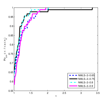
We now compare the performance of NMLS-G, NMLS-H, NMLS-N and NMLS-M, NMLS-1 and NMLS-2 using the directions (22) and (23). The test problems are those considered in the previous subsection. The related results are gathered in Tables 4 and 5. All considered algorithms are failed for some test problems in our implementation, $\mathtt{WASTON}$, $\mathtt{HARKAPER2}$, $\mathtt{POWER}$, $\mathtt{Extended~{}HILBERT}$, $\mathtt{FLETCHER}$, $\mathtt{CUBE}$ and $\mathtt{Generalized~{}White~{}and~{}Holst}$ for (22) and $\mathtt{CUBE}$ and $\mathtt{Generalized~{}White~{}and~{}Holst}$ for (23), so we delete them from Tables 4 and 5. The performance profile of the algorithms are demonstrated in Figures 8 and 9 for the measures $N_{g}$, $N_{f}$ and $N_{f}+3N_{g}$. Subfigures (a) and (b) of Figure 8 respectively illustrate the performance profile for $N_{g}$ and $N_{f}$ and indicate that the algorithms are comparable, however, NMLS-G and NMLS-H perform a little better regarding the number of function values. Subfigures (c) and (d) stand for the measure $N_{f}+3N_{g}$ with $\tau=1.5$ and $\tau=3$, respectively. They show that MNLS-H attains the most wins by about 58% and then NMLS-G by 57% while NMLS-N, NMLS-1 and NMLS-2 attain about 53% score of the wins and NMLS-M get the worst result by about 50%. Similarly, subfigures (a) and (b) of Figure 9 demonstrate the performance profile for $N_{g}$ and $N_{f}$, where they are comparable regarding the number of gradient evaluations, and NMLS-H and NMLS-G perform better regarding the number of function evaluations. Subfigures (c) and (d) of Figure 9 show that NMLS-H, MNLS-G and NMLS-1 attain the most wins by about 49%, 48% and 47% score, respectively.

(a)

(b)

(c)

(d)

Figure 8: Performance profiles of all considered algorithms measured by: (a) the number of iterations ($N_{i}$) or gradient evaluations ($N_{g}$); (b) the number of function evaluations ($N_{f}$); (c) and (d) the hybrid measure $N_{f}+3N_{g}$.

(a)

(b)

(c)

(d)

Figure 9: Performance profiles of all considered algorithms measured by: (a) the number of iterations ($N_{i}$) or gradient evaluations ($N_{g}$); (b) the number of function evaluations ($N_{f}$); (c) and (d) the hybrid measure $N_{f}+3N_{g}$.

Summarizing the results of this subsection, we see that the considered algorithms are comparable, however, NMLS-H and NMLS-G attain the best performance by using the direction (22), while NMLS-H, NMLS-G and NMLS-1 outperform the others by employing the direction (23).

3.4 Image deblurring/denoiding

Image blur is a common problem that frequently happens in the photography and often can ruin the photograph. In digital photography, the motion blur is caused by camera shakes, which is unavoidable in many situations. Hence image deblurring/denoising is one of the fundamental tasks in the context of digital imaging processing, aiming at recovering an image from a blurred/noisy observation. The problem is typically modelled as linear inverse problem

$$y=Ax+\omega,~{}~{}~{}x\in X,$$ (24)

where $X$ is a finite-dimensional vector space, $A$ is a blurring linear operator, $x$ is a clean image, $y$ is an observation, and $\omega$ is either Gaussian or impulsive noise.

The system of equations (24) is mostly underdetermined and ill-conditioned, and $\omega$ is not commonly available, so one is not able to solve it directly, see BerB; Neu. Hence, its solution is generally approximated by an optimization problem of the form

$$\begin{array}[]{ll}\mathrm{minimize}&~{}~{}\frac{1}{2}\|Ax-y\|_{2}^{2}+\lambda\varphi(x)\\ \mathrm{subject~{}to}&~{}~{}x\in X,\end{array}$$ (25)

where $\varphi$ is a smooth or nonsmooth regularizer such as $\varphi(x)=\frac{1}{2}\|x\|_{2}^{2}$, $\varphi(x)=\|x\|_{1}$, $\varphi(x)=\|x\|_{ITV}$, or $\varphi(x)=\|x\|_{ATV}$ in which $\|.\|_{ITV}$ and $\|.\|_{ATV}$ denote isotropic and anisotropic total variation, for more information see Aho; ChaCCNP and references therein. Among these regularizers, $\varphi(x)=\frac{1}{2}\|x\|_{2}^{2}$ is differentiable and the others are nondifferentiable. Therefore, by the aim of this paper to study differentiable objective function, we consider the next problem

$$\begin{array}[]{ll}\mathrm{minimize}&~{}~{}\frac{1}{2}\|Ax-y\|_{2}^{2}+\frac{\lambda}{2}\|Wx\|_{2}^{2}\\ \mathrm{subject~{}to}&~{}~{}x\in\mathbb{R}^{n},\end{array}$$ (26)

where $A,W\in\mathbb{R}^{m\times n}$ and $y\in\mathbb{R}^{m}$. It is assumed that $A^{T}A+\lambda W^{T}W$ is positive definite, i.e., the problem (26) is a strictly convex problem and has the unique optimizer $x^{*}\in\mathbb{R}^{n}$ for an arbitrary vector $y$.

We now consider the recovery of the $256\times 256$ blurred/noisy Lena image by minimizing the problem (26) using NMLS-G, NMLS-H, NMLS-N, NMLS-M, NMLS-1 and NMLS-2 with the search direction (23). The algorithms stopped after 25 iterations. In particular, we choose the blurring matrix $A\in\mathbb{R}^{n\times n}$ to be the out-of-focus blur with radius 3 and the regularization matrix $W$ to be the gradient matrix for the problem (26). Thus, the matrix $W^{T}W$ is the two-dimensional discrete Laplacian matrix. For both matrices, we exploit the Neumann boundary conditions, which usually gives less artifacts at the boundary, see MorPC; NgCT. The use of such boundary conditions means that $A^{T}A+\lambda W^{T}W$ is a block-Toeplitz-plus-Hankel matrix with Toeplitz-plus-Hankel blocks. The original and blurred/noisy version of Lena are demonstrated in Figure 10, and the recovered images by the considered algorithms of this image are depicted in Figure 12.

(a)

(b)

Figure 10: The $256\times 256$ original and blurred/noisy Lena images

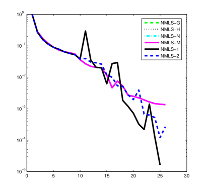
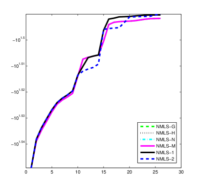
To see details of this experiment, we compare the function values and signal-to-noise improvement (ISNR) for the algorithms in Figure 11, where ISNR is defined by

$$\mathrm{ISNR}=20\log_{10}\left(\frac{\|y-x_{0}\|_{2}}{\|x_{b}-x_{0}\|_{2}}\right),$$

where $y$ is the observed image. Generally, this ratio measures the quality of the restored image $x_{b}$ relative to the blurred/noisy observation $y$. The subfigure (a) of Figure 11 shows that the algorithms perform comparable, while the subfigure (b) of Figure 11 indicates that NMLS-1 and NMLS-2 outperform the other algorithms regarding ISNR.

(a)

(b)

Figure 11: Deblurring of the $256\times 256$ blurred/noisy image by NMLS-G, NMLS-H, NMLS-N, NMLS-M, NMLS-1 and NMLS-2, where $rel.~{}:=(f_{k}-f^{*})/(f_{0}-f^{*})$ is the relative error of function values.

From Figure 12, it is observed that the algorithms recover the image in acceptable quality, where the last function value and PSNR are also reported. Here peak signal-to-noise (PSNR) is defined by

$$\mathrm{PSNR}=20\log_{10}\left(\frac{255n}{\|x_{b}-x_{0}\|_{2}}\right),$$

where $x_{b}$ is the approximated solution of (26) and $x_{0}$ is an initial point. This ratio is a common measure to assess the quality of the restored image $x_{b}$, i.e., it implies that NMLS-1 and NMLS-2 recover the blurred/noisy image better than the others.

(a)

(b)

(c)

(d)

(e)

(f)

Figure 12: Deblurring of the $256\times 256$ blurred/noisy image by NMLS-G, NMLS-H, NMLS-N, NMLS-M, NMLS-1 and NMLS-2. The algorithms were stopped after 25 iterations.

4 Conclusions and perspectives

This study first describes the motivation behind nonmonotone schemes, reviews the most popular nonmonotone terms and investigates the efficiency of them when they are incorporated into a backtracking Armijo-type line search in presence of some search directions. In particular, we propose two novel nonmonotone terms, combine them with Armijo’s rule and study their convergence. Afterwards, we report extensive numerical results and comparison among the two proposed nonmonotone schemes and some state-of-the-art nonmonotone line searches. The reported numerical results by using some measures of efficiency show that the performance of the considered nonmonotone line searches are varied depends on choosing search directions. Finally, employing the nonmonotone Armijo line searches for solving the dblurring problem produces acceptable results.

The experiments of this paper are limited to unconstrained optimization problems, however, the same experiments can be done for bound-constrained or general constrained optimization problems. We here consider only an Armijo-type line search, but one can investigate more numerical experiments with Wolfe-type or Goldestein-type line searches. For example studying of the behaviour of nonmonotone Wolfe-type line searches using conjugate-gradient directions is interesting. Furthermore, much more experiments on the parameters $\rho$ and $\delta$ for nonmonotone Armijo-type line searches can be done. It is also possible to extend our experiments to trust-region methods. One can consider many more applications with convex or nonconvex objective functions in the context of signal and image processing, machine learning, statistics and so on, which is out of the scope of this study.

Acknowledgement. We would like to thank Benedetta Morini that generously makes the codes of the paper MorPC available for us.

Appendix: Tables 1–5

Table 1. Numerical results with Newton’s direction
		NMLS-G		NMLS-H		NMLS-N		NMLS-M		NMLS-1		NMLS-2
Problem name	Dimension	$N_{i}$	$N_{f}$	$N_{i}$	$N_{f}$	$N_{i}$	$N_{f}$	$N_{i}$	$N_{f}$	$N_{i}$	$N_{f}$	$N_{i}$	$N_{f}$
Beale	2	17	25	14	27	17	25	14	27	13	22	16	28
Brown badly scaled	2	7	113	7	113	7	113	7	113	7	113	7	113
Powell badly scaled	2	4	89	4	89	4	89	4	89	4	89	4	89
Variably Dim	2	7	8	7	8	7	8	7	8	7	8	7	8
Watson	2	4	5	4	5	4	5	4	5	4	5	4	5
Box three-dim	3	8	9	8	9	8	9	8	9	8	9	8	9
Gaussian	3	1	2	1	2	1	2	1	2	1	2	1	2
Gulf r . and d.	3	39	46	43	47	39	46	37	47	41	55	39	46
Helical valley	3	21	22	20	24	21	22	20	24	14	19	14	17
Bro . a . Dennis	4	11	66	11	66	11	66	11	66	11	66	11	66
E. Rosenbrock	4	11	16	15	23	11	16	15	23	18	27	15	22
E. Powell singular	4	15	16	15	16	15	16	15	16	15	16	15	16
Penalty I	4	16	17	16	17	16	17	16	17	16	17	16	17
Penalty II	4	8	9	8	9	8	9	8	9	8	9	8	9
Trigonometric	4	8	12	8	12	8	12	8	12	8	12	8	12
Wood	4	29	33	27	31	29	33	31	43	33	48	29	38
Biggs EXP6	6	13	18	17	24	23	33	15	34	15	34	21	31
Chebyquad	6	11	17	10	17	11	17	10	17	10	17	11	17
Penalty II	10	29	30	29	30	29	30	29	30	29	30	29	30
Average		13.631	29.11	13.89	29.95	14.16	29.89	13.68	31.11	13.79	31.47	13.84	30.26

Table 2. Numerical results with the BFGS direction
		NMLS-G		NMLS-H		NMLS-N		NMLS-M		NMLS-1		NMLS-2
Problem name	Dimension	$N_{i}$	$N_{f}$	$N_{i}$	$N_{f}$	$N_{i}$	$N_{f}$	$N_{i}$	$N_{f}$	$N_{i}$	$N_{f}$	$N_{i}$	$N_{f}$
Beale	2	17	24	17	24	24	24	17	24	16	24	17	24
Brown badly scaled	2	18	60	14	57	43	68	48	72	48	72	48	72
Powell badly scaled	2	63	91	63	91	63	88	69	95	63	88	65	90
Variably Dim	2	5	13	5	13	5	13	5	13	5	13	5	13
Watson	2	9	21	9	21	9	21	9	21	9	21	9	21
Box three-dim	3	30	39	30	39	30	39	30	39	30	39	30	39
Gaussian	3	3	6	3	6	3	6	3	6	3	6	3	6
Gulf r . and d.	3	30	40	33	44	30	40	33	44	33	44	33	44
Helical valley	3	50	80	43	73	50	80	38	68	33	60	31	53
Bro . a . Dennis	4	26	80	24	79	26	80	24	79	24	79	24	79
E. Rosenbrock	4	73	89	72	94	73	89	62	85	56	85	70	96
E. Powell singular	4	31	51	36	57	31	51	36	57	24	47	36	57
Penalty I	4	1258	1356	543	659	462	522	479	552	482	546	482	546
Penalty II	4	14	21	14	21	14	21	14	21	12	20	14	21
Trigonometric	4	14	15	13	15	14	15	13	15	13	15	13	15
Wood	4	33	68	30	65	33	68	33	68	30	65	33	68
Biggs EXP6	6	45	58	39	47	45	58	43	58	43	58	45	60
Chebyquad	6	19	32	19	32	19	32	18	32	19	32	18	33
Penalty II	10	1492	1682	1412	1727	509	786	524	781	514	767	648	982
Average		248.46	294.31	186.08	243.38	114.08	161.62	115.23	163.85	112.08	160.08	124.92	178.38

Table 3. Numerical results with the LBFGS direction
		NMLS-G		NMLS-H		NMLS-N		NMLS-M		NMLS-1		NMLS-2
Problem name	Dimension	$N_{i}$	$N_{f}$	$N_{i}$	$N_{f}$	$N_{i}$	$N_{f}$	$N_{i}$	$N_{f}$	$N_{i}$	$N_{f}$	$N_{i}$	$N_{f}$
Beale	2	21	26	21	26	21	26	21	26	21	26	21	26
Brown badly scaled	2	11	15	11	15	11	15	11	15	11	15	11	15
Full Hess . FH1	2	31	37	31	36	31	39	31	36	31	36	31	36
Full Hess . FH2	2	7	10	7	10	7	10	7	10	7	10	7	10
Gaussian	3	4	7	4	7	4	7	4	7	4	7	4	7
Box three-dim	3	49	68	54	61	46	65	42	62	51	63	42	62
Gulf r . and d.	3	64	85	64	87	61	84	68	94	64	90	64	90
Staircase 1	4	10	15	10	15	10	15	10	15	10	15	10	15
Staircase 2	4	10	15	10	15	10	15	10	15	10	15	10	15
Bro . a . Dennis	4	31	50	31	50	31	50	31	50	31	50	31	50
wood	4	66	92	90	119	78	101	49	68	64	102	48	68
Biggs EXP66	6	72	117	67	93	70	105	70	116	62	92	69	115
Penalty II	10	767	1561	525	1155	420	1068	541	1255	430	1012	538	1215
Variably Dim	10	15	37	15	37	15	37	15	37	15	37	15	37
E . Powell Sin	16	62	75	85	162	61	72	61	72	57	69	57	69
Watson	31	1704	2037	1813	2377	754	1033	1844	2480	788	1144	764	1039
HARKERP2	50	8917	9824	50001	1461198	9722	27035	9430	15756	8233	13643	9521	12691
ARGLINB	100	11	49	11	49	3	25	3	25	3	25	3	25
Diagonal 3	100	55	62	55	62	55	62	55	62	55	62	55	62
E . Rosenbrock	100	98	152	91	174	90	131	82	179	81	178	81	178
Diagonal 2	500	97	98	97	98	97	98	97	98	97	98	85	87
DIXON3DQ	1000	2016	2019	2016	2019	1739	1772	1969	1979	2001	2016	2001	2016
E . Beal	1000	13	16	13	16	13	16	13	16	13	16	13	16
Fletcher	1000	21076	22370	4353	4626	4354	4710	4336	4843	3930	4447	3930	4447
G . Rosenbrock	1000	14358	21530	10241	15876	10438	16115	8516	14717	8376	14871	8375	14811
Par . Pert . Quadratic	1000	149	163	149	163	144	160	152	168	144	160	144	160
Hager	1000	42	46	42	46	42	46	42	46	42	46	42	46
BDQRTIC	1000	171	237	154	188	246	942	305	1889	196	727	196	727
BG2	1000	23	34	23	34	23	34	23	34	23	34	23	34
POWER	1000	9391	9412	9041	9063	8932	9029	7451	7518	8618	8706	8618	8706
Purt . Trid. Quadratic	5000	579	592	579	592	577	595	558	576	581	603	581	603
Al . Pert . Quadratic	5000	551	564	551	564	586	604	604	620	549	566	549	566
Pert . Quadratic diag	5000	684	847	836	1049	807	1146	728	931	739	980	756	1001
E . Hiebert	5000	2368	6491	2103	4723	2224	5184	2040	5119	2017	5229	1987	5067
Fletcher	5000	12792	15151	50001	51822	25614	29246	18879	21076	17310	19750	17310	19750
E . Trid . 1	5000	22	25	22	25	22	25	22	25	22	25	22	25
NONSCOMP	5000	928	1852	2235	4504	1778	4391	1653	3832	1566	3684	1878	4596
LIARWHD	5000	63	114	71	91	60	112	41	65	41	65	42	67
CUBE	5000	2722	5079	9060	18506	8910	22743	7743	18930	8433	20787	8433	20787
TRIDIA	5000	1904	1917	1904	1917	1673	1695	1901	1927	1641	1666	1641	1666
DIXMAANA	9000	10	14	10	14	10	14	10	14	10	14	10	14
DIXMAANB	9000	8	12	8	12	8	12	8	12	8	12	8	12
DIXMAANC	9000	9	14	9	14	9	14	9	14	9	14	9	14
DIXMAAND	9000	10	16	10	16	10	16	10	16	10	16	10	16
DIXMAANE	9000	376	380	376	380	390	403	382	387	382	387	382	387
DIXMAANF	9000	268	272	268	272	251	258	261	268	261	268	261	268
DIXMAANG	9000	229	234	229	234	229	237	229	235	223	230	223	230
DIXMAANH	9000	223	229	223	229	233	243	229	236	229	236	229	236
DIXMAANI	9000	2798	2802	2798	2802	2653	2698	2801	2818	2751	2780	2751	2780
DIXMAANJ	9000	420	424	420	424	431	437	433	439	433	440	433	440
DIXMAANK	9000	361	366	361	366	377	385	361	366	361	366	361	366
DIXMAANL	9000	321	327	321	327	340	350	321	327	321	327	321	327
ARWHEAD	10000	13	30	13	30	13	30	13	30	13	30	13	30
BDEXP	10000	34	35	34	35	34	35	34	35	34	35	34	35
Broyden Tridiagonal	10000	50	55	53	59	50	55	50	55	53	59	50	55
COSIN	10000	26	28	15	19	26	28	15	19	15	19	15	19
Diagonal 4	10000	6	13	6	13	6	13	6	13	6	13	6	13
Diagonal 5	10000	5	6	5	6	5	6	5	6	5	6	5	6
Ext . Tridiagonal 2	10000	29	32	29	32	30	36	29	32	29	32	29	32
Diagonal 7	10000	5	7	5	7	5	7	5	7	5	7	5	7
Diagonal 8	10000	5	8	5	8	5	8	5	8	5	8	5	8
DQDRTIC	10000	10	19	10	19	10	19	10	19	10	19	10	19
ENGVAL1	10000	45	74	37	51	37	51	37	51	37	54	27	42
EDENSCH	10000	22	27	22	27	22	27	22	27	22	27	22	27
Ext . BD1	10000	14	17	13	15	14	17	12	16	13	15	12	16
Ext . DENSCHNB	10000	6	9	6	9	6	9	6	9	6	9	6	9
Ext . DENSCHNF	10000	14	23	14	23	14	23	14	23	14	23	14	23
Ext . Himmelblau	10000	9	16	9	16	9	16	9	16	9	17	9	16
Ext . Maratos	10000	219	558	221	452	228	473	192	436	188	424	205	479
Ext . Powell	10000	81	94	91	168	81	94	74	85	71	83	71	83
Ext . Penalty	10000	111	160	173	353	115	137	115	137	115	137	115	137
Ext . PSC1	10000	11	17	11	17	11	17	11	17	11	17	11	17
Ext . QP1	10000	25	41	25	41	25	41	25	41	25	41	25	41
Ext . QP2	10000	132	199	88	121	107	200	110	199	99	189	99	189
Ext . TET	10000	9	13	9	13	9	13	9	13	9	13	9	13
Ext . Wood	10000	68	94	90	115	79	102	50	69	66	104	50	70
Ext . White a . Holst	10000	83	123	53	86	81	116	73	134	68	117	61	95
Ext . Tridiagonal 1	10000	22	25	22	25	22	25	22	25	22	25	22	25
FH3	10000	4	19	4	19	4	19	4	19	4	19	4	19
G . PSC1	10000	45	52	45	52	45	52	45	52	45	52	45	52
G . Tridiagonal	10000	20	24	20	24	20	24	20	24	20	24	20	24
HIMMELBG	10000	2	3	2	3	2	3	2	3	2	3	2	3
NONDQUAR	10000	2081	2233	2055	2231	2167	2584	1973	2271	2043	2340	2043	2340
Perturbed	10000	835	849	835	849	837	857	789	810	835	854	835	854
QUARTC	10000	1	4	1	4	1	4	1	4	1	4	1	4
QF1	10000	839	852	839	852	841	861	834	853	880	900	880	900
QF2	10000	946	960	946	960	949	973	926	946	888	914	888	914
Raydan	10000	7	8	7	8	7	8	7	8	7	8	7	8
SINCOS	10000	11	17	11	17	11	17	11	17	11	17	11	17
TRIDIA	10000	2884	2898	2884	2898	3038	3079	3023	3054	2446	2479	2328	2355
Average		1063.51	1306.92	1780.31	17738.19	1040.96	1597.82	923.33	1327.82	0883.30	1282.16	900	1278.77

Table 4. Numerical results with the Barzilai-Borwein direction (BB1)
		NMLS-G		NMLS-H		NMLS-N		NMLS-M		NMLS-1		NMLS-2
Problem name	Dimension	$N_{i}$	$N_{f}$	$N_{i}$	$N_{f}$	$N_{i}$	$N_{f}$	$N_{i}$	$N_{f}$	$N_{i}$	$N_{f}$	$N_{i}$	$N_{f}$
Beale	2	46	52	42	50	46	53	36	52	38	54	37	54
Brown badly scaled	2	Failed	Failed	8	109	8	109	8	109	8	109	8	109
Full Hess . FH1	2	49	56	43	46	50	75	40	57	42	52	41	53
Full Hess . FH2	2	9	10	9	10	9	10	9	10	9	10	9	10
Gaussian	3	4	14	4	14	4	14	4	14	4	14	4	14
Box three-dim	3	36	62	36	64	36	67	105	219	882	1854	882	1854
Gulf r . and d.	3	1679	4232	2027	5724	4697	16171	43749	118335	36528	99453	2276	6860
Staircase 1	4	13	14	13	14	13	14	13	14	13	14	13	14
Staircase 2	4	13	14	13	14	13	14	13	14	13	14	13	14
Bro . a . Dennis	4	52	56	57	68	52	56	49	62	52	67	49	62
wood	4	242	326	138	154	255	520	1055	2291	222	450	805	1705
Biggs EXP66	6	567	904	1025	1826	4003	9631	3559	7571	3517	7309	4058	8536
Penalty II	10	579	1271	674	1518	2756	7686	1792	4497	1623	3997	1165	2954
Variably Dim	10	1	2	1	2	1	2	1	2	1	2	1	2
E . Powell Sin	16	214	348	145	213	5097	11888	1820	3812	2711	5493	2575	5284
ARGLINB	100	1075	41863	31	592	31	592	31	592	31	592	31	592
Diagonal 3	100	102	119	107	109	106	147	105	150	113	166	103	145
E . Rosenbrock	100	96	208	44	79	63	131	36	82	33	67	36	82
Diagonal 2	500	108	132	111	131	99	156	112	181	130	216	109	177
DIXON3DQ	1000	31289	52569	36487	66657	27809	65253	40299	86697	37983	80702	37983	80702
E . Beal	1000	48	55	41	49	48	55	36	56	35	45	36	55
Fletcher	1000	26718	44020	28940	51865	32507	74158	40440	85575	14475	29456	35721	74592
G . Rosenbrock	1000	24999	38314	24573	41178	23971	40964	25895	50162	25741	49242	26089	50267
Par . Pert . Quadratic	1000	203	270	179	180	305	590	325	592	411	711	433	731
Hager	1000	61	66	57	59	54	65	55	60	57	59	57	59
BDQRTIC	1000	82	91	86	87	80	94	81	106	87	98	69	74
BG2	1000	44	58	99	159	65	88	196	433	57	104	209	464
Purt . Trid. Quadratic	5000	2092	3344	854	1382	1633	3121	1685	3404	1765	3558	1727	3536
Al . Pert . Quadratic	5000	1602	2522	1831	3170	1026	1866	1956	3999	2052	4097	1117	2192
Pert . Quadratic diag	5000	362	595	470	797	1439	4045	1285	3160	1231	2900	977	2330
E . Trid . 1	5000	32	37	32	33	36	47	35	50	31	33	34	42
NONSCOMP	5000	62	63	62	63	54	56	54	57	63	65	54	57
LIARWHD	5000	50	80	45	101	63	122	66	191	40	87	53	139
TRIDIA	5000	8165	13522	11603	21006	10306	21041	14720	31687	17699	37371	14839	31400
DIXMAANA	9000	9	10	9	10	9	10	9	10	9	10	9	10
DIXMAANB	9000	8	9	8	9	8	9	8	9	8	9	8	9
DIXMAANC	9000	10	11	10	11	10	11	10	11	10	11	10	11
DIXMAAND	9000	13	14	13	14	13	14	13	14	13	14	13	14
DIXMAANE	9000	1177	1807	987	1695	821	1831	1061	2176	1039	2081	1023	1986
DIXMAANF	9000	442	675	715	1191	666	1449	641	1335	895	1800	1051	2076
DIXMAANG	9000	1024	1602	835	1377	734	1612	461	903	1022	2031	732	1457
DIXMAANH	9000	658	1030	924	1528	776	1706	754	1522	966	1929	878	1726
DIXMAANI	9000	6918	11583	6719	12096	6289	14861	10180	22178	7951	16803	9165	19375
DIXMAANJ	9000	580	857	475	725	819	1706	661	1239	896	1685	575	1080
DIXMAANK	9000	483	741	636	1020	618	1250	853	1703	596	1087	841	1604
DIXMAANL	9000	379	552	437	644	607	1244	660	1209	629	1176	477	890
ARWHEAD	10000	3	4	3	4	3	4	3	4	3	4	3	4
BDEXP	10000	18	19	18	19	18	19	18	19	18	19	18	19
Broyden Tridiagonal	10000	78	83	71	72	83	98	78	100	72	78	75	96
COSIN	10000	Failed	Failed	33	40	Failed	Failed	33	40	33	40	Failed	Failed
Diagonal 4	10000	3	4	3	4	3	4	3	4	3	4	3	4
Diagonal 5	10000	4	5	4	5	4	5	4	5	4	5	4	5
Ext . Tridiagonal 2	10000	31	36	31	36	30	36	31	36	31	36	31	36
Diagonal 7	10000	7	8	7	8	7	8	7	8	7	8	7	8
Diagonal 8	10000	6	8	6	8	6	8	6	8	6	8	6	8
DQDRTIC	10000	27	28	27	28	27	28	27	28	27	28	27	28
ENGVAL1	10000	28	29	28	29	28	29	28	29	28	29	28	29
EDENSCH	10000	27	28	27	28	27	28	27	28	27	28	27	28
Ext . BD1	10000	16	19	16	19	16	19	16	19	16	20	16	19
Ext . DENSCHNB	10000	10	11	10	11	10	11	10	11	10	11	10	11
Ext . DENSCHNF	10000	12	13	12	13	12	13	12	13	12	13	12	13
Ext . Himmelblau	10000	15	18	15	18	15	18	15	18	15	18	15	18
Ext . Maratos	10000	76	127	64	124	101	209	78	202	129	340	85	217
Ext . Powell	10000	360	674	231	397	14866	35239	6512	13509	6920	14447	4413	9095
Ext . Penalty	10000	123	2858	6	67	6	67	6	67	6	67	6	67
Ext . PSC1	10000	17	18	17	18	17	18	17	18	17	18	17	18
Ext . QP1	10000	13	14	13	14	13	14	13	14	10	14	13	14
Ext . QP2	10000	51	106	35	73	26	54	23	47	15	30	25	48
Ext . TET	10000	10	13	10	13	10	13	10	13	10	13	10	13
Ext . Wood	10000	274	365	139	155	281	575	1157	2464	242	464	1163	2474
Ext . White a . Holst	10000	122	157	76	116	103	168	68	154	66	141	68	154
Ext . Tridiagonal 1	10000	32	37	35	37	36	47	36	51	31	33	34	42
FH3	10000	3	4	3	4	3	4	3	4	3	4	3	4
G . PSC1	10000	26	27	26	27	26	27	26	27	26	27	26	27
G . Tridiagonal	10000	26	27	26	27	26	27	26	27	26	27	26	27
HIMMELBG	10000	20	21	20	21	20	21	20	21	20	21	20	21
NONDQUAR	10000	5734	9701	6121	11539	10738	25859	8646	18582	9890	21268	9310	19820
Perturbed	10000	3332	5371	1996	3418	3028	6319	3610	7646	2894	5941	3096	6337
QUARTC	10000	1	2	1	2	1	2	1	2	1	2	1	2
QF1	10000	1914	3035	3367	6017	3070	6296	3901	8223	3339	6896	2887	5878
QF2	10000	1853	3020	1857	3161	2424	4866	2269	4724	2398	4889	3277	6715
Raydan	10000	1	2	1	2	1	2	1	2	1	2	1	2
SINCOS	10000	17	18	17	18	17	18	17	18	17	18	17	18
TRIDIA	10000	21252	35581	28315	51638	18599	38133	24617	52700	25154	53422	30126	64210
Average		2951.65	27514.52	1956.45	3512.77	2759.61	9558.57	2932.75	6493.89	2538.79	5542.02	2991.69	6378.95

Table 5. Numerical results with the Barzilai-Borwein direction (BB2)
		NMLS-G		NMLS-H		NMLS-N		NMLS-M		NMLS-1		NMLS-2
Problem name	Dimension	$N_{i}$	$N_{f}$	$N_{i}$	$N_{f}$	$N_{i}$	$N_{f}$	$N_{i}$	$N_{f}$	$N_{i}$	$N_{f}$	$N_{i}$	$N_{f}$
Beale	2	30	31	30	31	30	31	31	36	30	35	32	37
Brown badly scaled	2	Failed	Failed	8	109	8	109	8	109	8	109	8	109
Full Hess . FH1	2	38	40	38	40	33	40	38	41	38	44	33	40
Full Hess . FH2	2	9	10	9	10	9	10	9	10	9	10	9	10
Gaussian	3	4	14	4	14	4	14	4	14	4	14	4	14
Box three-dim	3	72	91	75	89	71	93	72	91	71	91	72	91
Gulf r . and d.	3	532	578	762	848	531	633	645	737	690	800	631	742
Staircase 1	4	7	8	7	8	7	8	7	8	7	8	7	8
Staircase 2	4	7	8	7	8	7	8	7	8	7	8	7	8
Bro . a . Dennis	4	49	50	49	50	49	50	49	50	49	50	47	51
wood	4	581	704	705	808	552	653	638	793	602	750	758	953
Biggs EXP66	6	453	495	413	457	605	702	590	661	536	597	473	529
Penalty II	10	223	301	73	76	329	446	433	556	333	436	421	536
Variably Dim	10	1	2	1	2	1	2	1	2	1	2	1	2
E . Powell Sin	16	133	152	120	131	162	220	134	175	140	184	156	205
Watson	31	4961	5148	7062	7312	5216	5606	6798	7100	7677	8102	6079	6472
HARKERP2	50	27851	28183	Failed	Failed	15438	18678	32888	33460	34703	36001	23470	24294
ARGLINB	100	1069	40515	30	591	30	591	30	591	30	591	30	591
Diagonal 3	100	92	93	92	93	108	114	116	121	116	121	116	121
E . Rosenbrock	100	58	65	58	65	64	73	78	95	73	100	74	102
Diagonal 2	500	112	115	103	105	134	145	92	101	115	120	104	120
DIXON3DQ	1000	8286	8363	9367	9488	10934	11188	6567	6654	6856	6958	6567	6654
E . Beal	1000	28	29	28	29	28	29	28	32	28	32	30	36
Fletcher	1000	4569	5626	8089	9784	4445	5550	11476	13223	11407	13141	11385	13112
G . Rosenbrock	1000	24950	28069	23700	26822	23814	26980	23673	26804	25645	28796	23797	26941
Par . Pert . Quadratic	1000	218	233	212	217	244	269	308	328	314	342	314	342
Hager	1000	48	50	48	50	48	50	48	50	48	50	48	50
BDQRTIC	1000	88	89	88	89	93	98	96	100	82	88	82	88
BG2	1000	55	60	55	60	79	99	68	78	75	99	100	118
POWER	1000	29416	29678	14753	14914	27012	27355	28046	28376	25356	25678	21596	21839
Purt . Trid. Quadratic	5000	981	1009	825	852	932	1002	1021	1059	1318	1381	780	817
Al . Pert . Quadratic	5000	840	866	1136	1173	1019	1095	954	1009	935	991	954	1009
Pert . Quadratic diag	5000	273	299	308	312	357	430	299	332	308	353	332	368
E . Hiebert	5000	3181	3185	3181	3185	3181	3185	3181	3185	3181	3185	3181	3185
Fletcher	5000	23321	28385	22936	31043	Failed	Failed	17180	25290	18139	26278	17864	25970
E . Trid . 1	5000	31	32	31	32	31	32	31	32	31	32	31	32
NONSCOMP	5000	47	48	47	48	47	48	47	48	47	48	47	48
LIARWHD	5000	54	55	49	53	49	51	55	71	44	57	47	64
TRIDIA	5000	4804	4913	4076	4162	3574	3685	4319	4409	5477	5634	3334	3430
DIXMAANA	9000	9	10	9	10	9	10	9	10	9	10	9	10
DIXMAANB	9000	8	9	8	9	8	9	8	9	8	9	8	9
DIXMAANC	9000	10	11	10	11	10	11	10	11	10	11	10	11
DIXMAAND	9000	13	14	13	14	13	14	13	14	13	14	13	14
DIXMAANE	9000	537	551	622	647	483	537	853	883	764	792	809	848
DIXMAANF	9000	631	637	478	502	473	509	473	489	521	543	312	328
DIXMAANG	9000	527	543	374	382	589	638	595	612	337	361	337	361
DIXMAANH	9000	564	585	678	693	419	453	594	609	500	520	522	550
DIXMAANI	9000	2608	2650	3197	3239	3815	3965	3450	3522	2898	2979	3152	3226
DIXMAANJ	9000	531	546	605	622	634	667	394	404	394	415	406	417
DIXMAANK	9000	364	374	416	428	410	438	395	410	369	389	510	527
DIXMAANL	9000	365	377	435	452	396	424	379	399	324	348	400	420
ARWHEAD	10000	3	4	3	4	3	4	3	4	3	4	3	4
BDEXP	10000	18	19	18	19	18	19	18	19	18	19	18	19
Broyden Tridiagonal	10000	92	95	99	100	97	103	98	109	110	116	97	110
COSIN	10000	Failed	Failed	35	44	Failed	Failed	40	50	35	44	40	65
Diagonal 4	10000	3	4	3	4	3	4	3	4	3	4	3	4
Diagonal 5	10000	4	5	4	5	4	5	4	5	4	5	4	5
Ext . Tridiagonal 2	10000	33	38	33	38	37	44	33	38	33	38	33	38
Diagonal 7	10000	7	8	7	8	7	8	7	8	7	8	7	8
Diagonal 8	10000	6	8	6	8	6	8	6	8	6	8	6	8
DQDRTIC	10000	21	22	21	22	21	22	21	22	21	22	21	22
ENGVAL1	10000	31	32	31	32	31	32	31	32	31	32	31	32
EDENSCH	10000	30	31	30	31	30	31	30	31	30	31	30	31
Ext . BD1	10000	15	18	15	18	15	18	15	18	14	18	15	18
Ext . DENSCHNB	10000	10	11	10	11	10	11	10	11	10	11	10	11
Ext . DENSCHNF	10000	13	14	13	14	13	14	13	14	13	14	13	14
Ext . Himmelblau	10000	15	17	15	17	15	17	15	17	15	17	15	17
Ext . Maratos	10000	119	144	115	141	119	144	136	182	135	185	136	182
Ext . Powell	10000	194	226	166	185	187	241	202	273	186	256	243	318
Ext . Penalty	10000	122	2857	5	66	5	66	5	66	5	66	5	66
Ext . PSC1	10000	14	15	14	15	14	15	14	15	14	15	14	15
Ext . QP1	10000	13	14	13	14	13	14	13	14	10	14	13	14
Ext . QP2	10000	51	106	35	73	26	54	23	47	15	30	23	47
Ext . TET	10000	9	12	9	12	9	12	9	12	9	12	9	12
Ext . Wood	10000	607	726	695	804	551	658	691	866	662	845	825	1047
Ext . White a . Holst	10000	66	68	71	72	66	68	88	107	72	89	88	108
Ext . Tridiagonal 1	10000	33	35	34	35	33	37	33	35	33	37	33	37
FH3	10000	3	4	3	4	3	4	3	4	3	4	3	4
G . PSC1	10000	26	27	26	27	26	27	26	27	26	27	26	27
G . Tridiagonal	10000	24	25	24	25	24	25	24	25	24	25	24	25
HIMMELBG	10000	21	22	21	22	21	22	21	22	21	22	21	22
NONDQUAR	10000	2856	2916	2976	3035	3025	3193	2986	3068	2888	2999	2996	3092
Perturbed	10000	1599	1650	1298	1337	1612	1732	1480	1525	2074	2156	1462	1524
QUARTC	10000	1	2	1	2	1	2	1	2	1	2	1	2
QF1	10000	1043	1097	1909	1961	1636	1714	1259	1313	1854	1925	1282	1339
QF2	10000	1525	1576	1738	1786	1482	1557	1388	1449	1326	1402	1260	1321
Raydan	10000	1	2	1	2	1	2	1	2	1	2	1	2
SINCOS	10000	14	15	14	15	14	15	14	15	14	15	14	15
TRIDIA	10000	9767	9898	5519	5625	5839	5976	5073	5157	5742	5893	10527	10712
Average		2944.38	24306.72	1915.18	2100.42	2489.36	2685.27	1809.83	1998.06	1866.80	2068.75	1672.60	1867.37