Understanding the Formation and Evolution of Interstellar Ices: A Bayesian Approach

Abstract

Understanding the physical conditions of dark molecular clouds and star forming regions is an inverse problem subject to complicated chemistry that varies non-linearly with time and the physical environment. In this paper we apply a Bayesian approach based on a Markov Chain Monte Carlo (MCMC) method for solving the non-linear inverse problems encountered in astrochemical modelling. We use observations for ice and gas species in dark molecular clouds and a time dependent, gas grain chemical model to infer the values of the physical and chemical parameters that characterize quiescent regions of molecular clouds. We show evidence that in high dimensional problems, MCMC algorithms provide a more efficient and complete solution than more classical strategies. The results of our MCMC method enable us to derive statistical estimates and uncertainties for the physical parameters of interest as a result of the Bayesian treatment.

1 INTRODUCTION

Molecular clouds are regions where extinction by dust is high ($A_{V}\gtrsim$5 mag), temperatures are low ($\sim$ 10 K), densities are high ($n_{\rm H}$ $\geq$ 10³ cm^-3) and where most of the gas is molecular. They contain higher ($>$ 10⁴ cm^-3) density structures (Myers & Benson, 1983), some of which may become gravitationally unstable and initiate the early stages of star formation. Understanding the life cycle of dark molecular clouds is very important for comprehending star formation and for getting insight into the processes of the interstellar medium and to that extend galaxy formation. Molecules provide a paramount tool for the analysis of the chemical and physical conditions of star forming regions. Every stellar or planetary evolutionary stage is characterized by a chemical composition, which represents the physical processes of its phase.

In the dense cores of molecular clouds, molecules and atoms previously in the gas phase, deplete onto the dust grains. For each atom or molecule, freeze out (or depletion) depends on a complicated time dependent, non linear chemistry that strongly depends on the physical environment. It is difficult to quantify depletion observationally (e.g. Christie et al., 2012). CO emission can be used to infer the fraction of species that is in the form of icy mantles, by taking the ratio of the observed CO to the expected abundance at a particular density in steady state, if freeze out did not occur (e.g. Caselli et al., 1999). This however, not only implies that the cores are in steady-state, but also implies a knowledge of the H₂ density, as well as of the efficiency of the non thermal desorption mechanisms that can return the depleted CO to the gas. Moreover, the CO depletion factor is not necessarily equivalent to the molecular gas depletion factor, because different species freeze and desorb at different rates with different sticking coefficients, which are mostly unknown.

The detection of water ice mantles in cold dark interstellar clouds and star forming regions (Öberg et al., 2011) provides us with direct evidence that surface reactions on dust grains involving oxygen atoms make water molecules, which are then retained on the surface and make water ice. Not all species undergo surface reactions when they stick to dust grains. For example, CO sticks efficiently to surfaces at temperatures below $\sim$ 25 K and is found to be abundant in the ices. Some of this CO can be converted to other species.

The relatively high abundance of CO₂, CH₃OH, and H₂CO in ices (Öberg et al., 2011; Whittet et al., 2011), relative to H₂O, in some clouds indeed suggest that some processing of CO to these products is occurring, due possibly by irradiation, by cosmic rays or by photons generated by cosmic rays inside the cloud. H₂CO and CH₃OH are stages in the surface hydrogenation of CO. Similarly, CO₂ can be the result of oxygenation of CO:

$$\rm{CO}+\rm{OH}\rightarrow\rm{CO}_{2}+\rm{H}$$

Some ices can be thermally returned to the gas phase when the gas temperature is higher than 20 K. At low gas temperatures non-thermal desorption processes can also return molecules from solid to gas-phase (e.g. Roberts et al. (2007)). However, these mechanisms ‘compete’ with those of freeze-out. The composition of the icy mantles is clearly a time-dependent process highly dependent on the initial conditions of the gas in any particular cloud. Hence, the ices on dust grain surfaces are of a mixed composition and may reflect the local conditions and evolutionary history. In some dark molecular clouds, the ices are abundant, indicating that non thermal desorption mechanisms may not be very efficient everywhere. The potential interconnection and linear or non-linear correlation of these parameters with each other or with extra unknown parameters augments our difficulty to determine and specify the parameter network. The large parameter space in combination with the number of parameters and the complexity of the physical system make the task of parameter estimation highly challenging.

The increasingly detailed observations of molecular clouds and star forming regions enable us to identify some of the most important processes at work. Chemical and radiative transfer models can transform molecular observations into powerful diagnostics of the evolution and distribution of the molecular gas. The results of these models though, depend on a number of parameters or group of parameters that are most of the times poorly constrained. Moreover, deriving information about molecular clouds using observational information and, even well established modeling codes, is an inverse problem that usually does not fulfill Hadamard’s (Hadamard, 1902) postulates of well-posedness. That is, it may not have a solution, solutions might not be unique and/or might not depend continuously on the observational data. The first and second postulates simply state that for a well-posed problem a solution should exist and be unique. The third postulate holds when small changes in the observational data result in small changes in the solution. As shown later in Section 3.1, in typical astrochemical problems, only the first postulate holds and we usually have to deal with non linear ill-posed inverse problems.

Employing sampling algorithms is a traditional approach to tackle inverse problems in many scientific fields with large parameter space. Bayesian statistical techniques and Monte Carlo sampling methods such as Markov Chain Monte Carlo (MCMC) algorithms and Nested Sampling have flourished over the past decade in astrophysical data analysis (Christensen & Meyer, 2000; Ford, 2005; Fitzgerald et al., 2007; Feroz & Hobson, 2008; Isella et al., 2009). A summary of a typical MCMC method and an application to quantify uncertainty in stellar parameters using stellar codes is given by Bazot et al. (2012). To our knowledge, MCMC methods have never been applied in the framework of parameter estimation through astrochemical modeling. In this paper we present a first astrochemical application of gas-grain chemical modeling, molecular abundances and a Bayesian statistical approach based on MCMC methodology.

The motivation of the present paper is to solve the inverse problem of deriving the physical conditions in interstellar molecular clouds; in particular: the gas density, cosmic ray ionization rate, radiation field, the rate of collapse, the freeze-out rate and non-thermal desorption efficiency. In Section 2, we formulate a typical inverse problem for interstellar molecular clouds and describe the bayesian method and the Metropolis-Hastings (MH) algorithm (an example of a wider class of MCMC techniques). In Section 3, we discuss the statistical results and the astrophysical consequences. Finally in Section 4, we present our conclusions.

2 PARAMETER ESTIMATION

In this paper, we are interested in dense, cold, quiescent regions of molecular clouds where atoms and molecules in the gas phase freeze-out on to the dust grains. The observed quantities are molecular abundances for solid and gas phase species. The parameters we want to estimate are the cloud density $n_{H}$, the cosmic ray ionization rate $\zeta$, radiation field rate $G_{\circ}$, the cloud collapse rate $C_{f}$ and three non thermal desorption efficiencies $\epsilon$, $\phi$, $y$ presented in Section 2.3. Due to the nature of the addressed inverse problem, the theoretical and modeled relationship between the parameters and the observed data is highly non-linear. Therefore, we anticipate several degeneracies as well as a multi-modal and non-Gaussian joint parameter distribution. Moreover, the parameters are not uniquely related to the observations. While the forward problem has (in deterministic physics) a unique solution, the inverse problem does not. Different combinations of parameters can produce the same abundances. Furthermore, the possible combinations of parameters are too many to permit an exhaustive search.

Traditional approaches to tackle inverse problems of this nature fail to cope with these kind of issues. Methods based on searching iteratively to minimize an appropriate distance such as the $\rm{\chi}^{2}$ error, can be stuck in local minimum and give degenerate solutions. Alternative approaches to aim for a global solution such as simulated annealing would have some benefits, but since we are not just looking for the global optimum of our target distribution, the most comprehensive view is obtained by a Bayesian Monte Carlo sampling method. We selected the Bayesian MCMC approach against other methods that work equally well with complex and multimodal target distributions (e.g. Nested Sampling), since MCMC constitutes a benchmark algorithm in Monte Carlo sampling and parameter estimation problems.

To overcome the challenges of an ill-posed nonlinear inverse problem we adopted a Bayesian approach based on the use of Metropolis-Hastings (MH) algorithm. The Bayesian framework for inverse problems is based on systematic modeling of all errors and uncertainties from the Bayesian viewpoint. The potential of this approach to solve difficult inverse problems with high noise levels and serious model uncertainties is much higher and also allows for prior information to be incorporated. The Bayesian solution is the whole posterior distribution of the parameters and therefore, there is not only one solution, but a set of possible values. The advantage of MCMC approach is that there is no restriction concerning the non-linearity of the model. Moreover, an appropriate tuning of the MCMC parameters allows the algorithm to explore all modes of the target distribution. Finally, even though it is still not feasible to do an exhaustive search through the parameter space, MCMC methods can effectively explore the parameters’ joint posterior distribution, since model computations are concentrated around regions of interest in the parameters space.

2.1 Bayesian Inverse Problem

Our aim is to obtain information about physical parameters of a molecular cloud $\boldsymbol{\theta}=(\theta_{1},\theta_{2},...,\theta_{k})$, while we measure molecular abundances $\boldsymbol{\mathcal{Y}}=(\mathcal{Y}_{1},\mathcal{Y}_{2},...,\mathcal{Y}_{n})$. These quantities are related to a (forward) function $f(\cdot)$ which represents the physical and chemical processes in the cloud. The main challenge is that there is no closed form function $f$ mapping the parameters to the observations, which could be inverted. However, given a set of parameters, estimated abundance values for the species of interest can be computed with astrochemical models denoted here as $\mathcal{C}(\cdot)$. The addressed problem in our case is how to estimate $\boldsymbol{\theta}$ from

$$\boldsymbol{\mathcal{Y}}=\mathcal{C}(\boldsymbol{\theta})+\boldsymbol{\varepsilon}$$ (1)

and according to Idier (2008) this constitutes an inverse problem. The error term $\boldsymbol{\varepsilon}$, represents both the observational noise and the modeling error between $\mathcal{C}(\cdot)$ and $f(\cdot)$.

We treat $\boldsymbol{\mathcal{Y}}$, $\boldsymbol{\theta}$ and $\boldsymbol{\varepsilon}$ as random variables and define the “solution” of the inverse problem to be the posterior probability distribution of the parameters given the observations. This allows to model the noise via its statistical properties, even though we do not know the exact instance of the noise entering our data. We can also optionally specify a priori the form of solutions that we believe to be more likely, through a prior distribution. Thereby, we can attach weights to multiple solutions which explain the data. This is the Bayesian approach to inverse problems.

Assume we have $K$ parameters $\theta_{k}$ and $N$ solid phase observable quantities $\mathcal{Y}_{n}$. The error $\varepsilon_{n}$ on each observation $\mathcal{Y}_{n}$ is assumed to be normally distributed with variance $\sigma_{n}^{2}$. In addition, it is assumed that the observational errors are independent. The $\sigma_{n}^{2}$ is considered to correspond to the uncertainty on $\mathcal{Y}_{n}$, which is solely dictated by the observation. The probability density function of the errors is given by:

$$p_{\varepsilon}(\boldsymbol{\varepsilon})=\prod_{n=1}^{N}\frac{1}{(2\pi)^{\frac{1}{2}}\sigma_{n}^{2}}\exp(\frac{\varepsilon_{n}^{2}}{2\sigma_{n}^{2}})$$

Using (1), we can define the likelihood function $\mathbb{L}$ of observations given a model parametrized by a set of parameters as

$$\mathbb{L}(\boldsymbol{\theta};\boldsymbol{\mathcal{Y}})=p_{\varepsilon}(\boldsymbol{\mathcal{Y}}-\mathcal{C}(\boldsymbol{\theta}))=\prod_{n=1}^{N}\frac{1}{(2\pi)^{\frac{1}{2}}\sigma_{n}^{2}}\times\exp(-\frac{1}{2}\sum_{n=1}^{N}[\frac{\mathcal{C}(\theta_{n})-\mathcal{Y}_{n}}{2\sigma_{n}}])$$

In case any prior information about the unknown parameters is available, the Bayesian approach allows for this information to be taken into account. This information can be integrated through a prior probability distribution on the parameters, say $\pi(\boldsymbol{\theta})$. Then parameter estimation can be performed through the posterior probability distribution (PPD), using Bayes’ rule

$$\pi(\boldsymbol{\theta}|\boldsymbol{\mathcal{Y}})=\frac{\mathbb{L}(\boldsymbol{\theta};\boldsymbol{\mathcal{Y}})\pi(\boldsymbol{\theta)}}{m(\boldsymbol{\mathcal{Y}})}$$ (2)

The PPD expresses our uncertainty about the parameters after considering the observations and any prior information. The denominator is simply a normalization factor.

In reality we are not able to access the whole posterior probability distribution. Therefore, computation of parameter estimates or uncertainties is a hard task. MCMC methods are efficient methods that allow to sample from complex probability distributions and approximate complex probability densities.

2.2 Markov Chain Monte Carlo

MCMC methods are a powerful class of algorithms that produce random samples distributed according to the distribution of interest. The importance and efficiency of MCMC methods lies in the fact that these samples can be used to approximate the probability density of the distribution by calculating it only for a feasible number of parameter values. Among the several implementations of possible algorithms, we employ a MH sampling algorithm (Gilks et al., 1995). The MH algorithm will enable us to explore the parameter space and approximate efficiently the PPD. A theoretical introduction on MCMC and MH is far beyond the scope of this paper. However, in Appendix A, we briefly describe the MH algorithm and how MCMC is employed for parameter estimation in our case. Note that the tuning of the MH algorithm as described in Appendix A is very crucial when aiming to approximate possibly multi-modal and non-Gaussian distribution, which is the case for this study.

2.3 Parameter Space

The chemical modeling code used in this paper and denoted as $\mathcal{C}(\cdot)$ in (1) is the UCL_CHEM time dependent gas-grain chemical code (Viti et al., 2004) and is briefly described in Appendix B and references therein. Note that for each set of parameters, $\mathcal{C}(\cdot)$ provide us with time series of chemical abundances. We choose to extract the chemical abundances of interest for the time points when the final density is reached and the cloud collapse has finished. Even though we ignore the previous time points, the time dependancy is still taken into account and investigated through exploration of different final density values.

The parameters for our chemical modeling code create a nine dimensional parameter space (9D) for molecular clouds as used in our MH and described in Table 1:

$$\boldsymbol{\theta}=(n_{H},\zeta,G_{\circ},C_{f},fr,\epsilon,\phi,y,r),$$

In a first attempt to employ a Bayesian approach for deriving branching ratios for poorly understood chemical reaction pathways, we also investigated the parameter $r$, which controls how much of the gas phase Oxygen turns into ice H₂O or ice OH. Parameter $r$ reflects the percentage of O that turns into H₂O, so that $1-r$ reflects the percentage of Oxygen that turns into OH. Desorption efficiencies resulting from H₂ formation on grains, direct cosmic ray heating and cosmic ray induced photodesorption are determined by parameters $\epsilon$, $\phi$ and $y$, as introduced and studied by Roberts et al. (2007). The freeze-out parameter in our code is effectively the sticking coefficient, a number in the range of $0-100\%$ that adjusts the rate per unit volume at which species deplete on the grain. For the free-collapse to a particular $n_{H}$ we used the modified formula of Rawlings et al. (1992), where parameter $C_{f}$ is considered to be a retardation factor with a value less than one, to roughly mimic the magnetic and/or rotational support, or an acceleration factor with a value greater than one to simulate a collapse faster than a free-fall (e.g. due to external pressure). Table 1 lists the set of physical parameters studied in this paper along with their definition domain $\mathbb{D}_{{\theta_{k}}}$. The joint definition domain $\mathbb{D}_{{\theta}}$ represents the parameter space to explore. The selected domain limits refer to the theoretical range of possible values for molecular clouds where atoms and molecules deplete on to the dust, ensuring though that extreme values are included.

2.4 Observational Constraints

The observational constraints of our analysis are based on data from the existing literature. Even though in this application we are primarily interested in ices, we include both gas phase and solid phase observations. To avoid confusion, we will denote with $\boldsymbol{\mathcal{Y}}$ a vector containing any observed quantity and if required we will specify whether we refer to solid phase or gas phase observations.

The solid phase observations include column densities and visual extinction data for molecular clouds in front of field stars. Such sources often provide suitable opportunities to observe and study ices in quiescent regions of the clouds (e.g. Boogert et al., 2011). We used 31 observations of H₂O, CH₃OH, CO and CO₂ from 31 different regions of 16 different clouds found in literature and summarized by Whittet et al. (2011). The data suggest some abundance variation, which was attributed to different evolutionary stages for different clouds. The scope of this paper lie beyond studying the behavior of a specific cloud, but rather on how to get statistical insight into the dynamics of common cloud classes. Therefore, the observational data is transformed into fractional abundances with respect to total H nuclei and then the average value is computed and used for our analysis.

In an attempt to minimize degeneracies we introduce additional gas phase abundances as an optional observational constraint. Due to the ill-posed nature of our problem, it is possible for our chemical model to end up with a solution space that fits perfectly the solid phase observations, but with gas phase abundances far from realistic. Hence, the addition of gas phase observations can be considered as a mathematical regularization by introducing additional prior information. Prior information can be naturally integrated into our Bayesian approach. The gas species observations were collected from more than one study, attempting to match the clouds, regions or evolutionary stage of the observational sources used for the solid phase species. If we were to fit observations of a particular source, then, ideally, every observational gas phase constraint should be able to contribute to the regularization of our methodology. However, as we are here only attempting at exploring a methodology, we found that three gas phase species were adequate to provide insight on the efficiency of gas phase species as a regularization factor. Abundances for NH₃ and N₂H⁺ were collected from Johnstone et al. (2010) while HCO⁺ from Schöier et al. (2002). The gas phase observations are in the form of fractional abundances with respect to total hydrogen nuclei. Table 2 lists the average molecular abundances for all the species along with their uncertainties. We emphasize again that the error on each of the observations $\mathcal{Y}_{n}$ is assumed to be normally distributed with a variance $\sigma_{n}^{2}$ that is determined solely by the uncertainty reported in Table 2.

2.5 Priors

We run two identical sets of 8 MCMC chains that differ on the prior distribution information. For the first set, the prior information is non-informative and in the form of acceptable range of possible values. Therefore, $\pi(\boldsymbol{\theta})$ is just uniformly distributed on $\mathbb{D}_{{\theta}}$, as listed in Table 1. Note that the observational data $\boldsymbol{\mathcal{Y}}$ refers only to the solid phase molecular abundances and in this case the gas phase species are ignored. In the second case, the prior information includes the observational constraints from the gas phase species as well. Let $\boldsymbol{\mathcal{Y}}$ now include all the observational constraints, $\boldsymbol{\mathcal{Y}}_{s}$ just the solid phase and $\boldsymbol{\mathcal{Y}}_{g}$ the gas phase observational constraints. In that case, the PPD is defined as:

$$\pi(\boldsymbol{\theta}|\boldsymbol{\mathcal{Y}})=\pi(\boldsymbol{\theta}|\boldsymbol{\mathcal{Y}}_{s},\boldsymbol{\mathcal{Y}}_{g})=\frac{\pi(\boldsymbol{\mathcal{Y}}_{s}|\boldsymbol{\theta},\boldsymbol{\mathcal{Y}}_{g})\pi(\boldsymbol{\theta}|\boldsymbol{\mathcal{Y}}_{g})}{m(\boldsymbol{\mathcal{Y}})}$$ (3)

The prior information is simply the likelihood function $\mathbb{L}(\cdot)$ of $\boldsymbol{\mathcal{Y}}_{g}$ given a model parametrized by $\boldsymbol{\theta}$, since:

$$\pi(\boldsymbol{\mathcal{Y}}_{s}|\boldsymbol{\theta},\boldsymbol{\mathcal{Y}}_{g}) =\mathbb{L}(\boldsymbol{\theta};\boldsymbol{\mathcal{Y}}_{s})$$

$$\pi(\boldsymbol{\theta}|\boldsymbol{\mathcal{Y}}_{g}) \propto\mathbb{L}(\boldsymbol{\theta};\boldsymbol{\mathcal{Y}}_{g})\pi(\boldsymbol{\theta)}$$

Including prior information in this way is equivalent to attaching weight to the solutions that explain the gas phase as well as the solid phase chemistry.

2.6 Blind Benchmark Test

In order to quantitatively investigate the effectiveness of our method to astrochemical problems we performed a benchmark test. This benchmark test is basically our Bayesian analysis applied this time on synthetic observations produced by UCL_CHEM using a pre-defined set of parameters $\boldsymbol{\theta_{T}}$. Once we have our synthetic observations, we apply our methodology and analyse the results and whether the true parameters are recovered. Knowing the solution to this test a priori, allows us not only to validate the method, but also to critically perceive the non linear and ill-posed nature of our problem. This discussion can be found in section 3.1. The reasoning behind the particular selection of parameters was a random choice not far from expected or well accepted values in the literature. The parameter values used in the test can be found in Table 3.

3 RESULTS

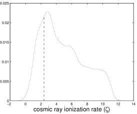
(a)

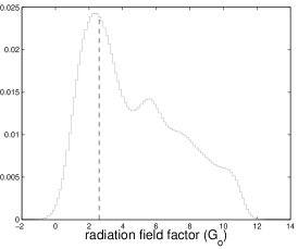
(b)

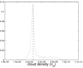
(c)

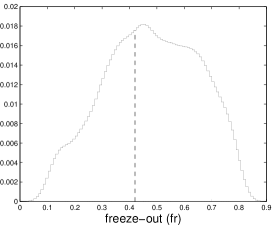
(d)

(e)

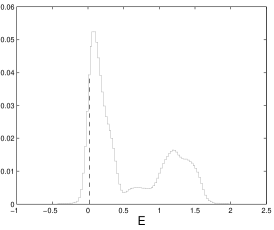
(f)

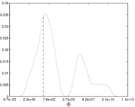
(g)

(h)

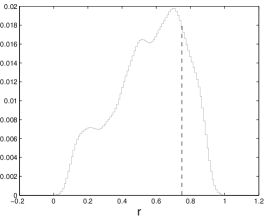
(i)

Figure 1: 1D Marginalized PPD for each of the nine parameters for the Blind Benchmark Test. The plots show the Gaussian kernel density estimator of each Probability Density Function. Dashed lines indicate the pre-defined parameter values $\boldsymbol{\theta_{T}}$ we wish to recover.

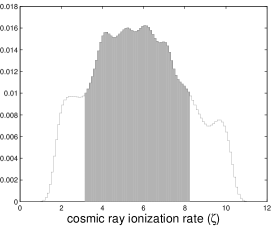
(a)

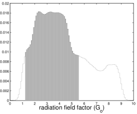
(b)

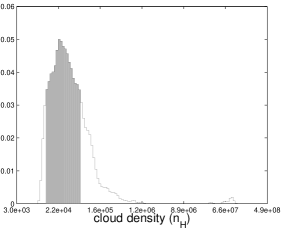
(c)

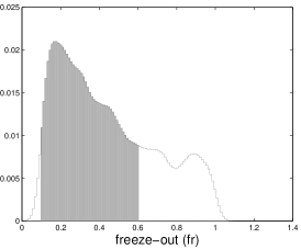
(d)

(e)

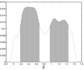
(f)

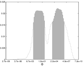
(g)

(h)

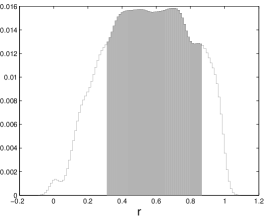
(i)

Figure 2: 1D Marginalized PPD for each of the nine parameters using uniform non informative prior. The plots show the Gaussian kernel density estimator of each Probability Density Function.Darker regions indicate $68\%$ HDR.

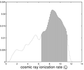
(a)

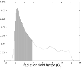
(b)

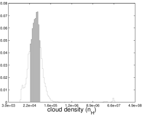
(c)

(d)

(e)

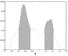
(f)

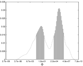
(g)

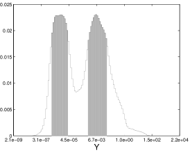
(h)

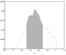
(i)

Figure 3: 1D Marginalized PPD for each of the nine parameters using informative prior from gas phase chemistry. The plots show the Gaussian kernel density estimator of each Probability Density Function. Darker regions indicate $68\%$ HDR.

When quoting parameter estimation results and especially multivariate results, it is convenient to decrease the parameter space to posterior intervals about single marginalized parameters. Figure  1 shows the nine 1D marginalized posterior probability distributions of the parameters for the benchmark test using a uniform prior. In Figure 2, we present the nine 1D marginalized posterior probability distributions of the parameters and their 68% High Density Regions (HDR), recovered from the uniform prior case. Figure 3, presents the same results for the informative prior case. HDR indicate the parameter space where the probability density is higher. We refer readers seeking more details about marginal posterior probability function and High Density Regions to Appendix C and references therein. In order to compare the 2 prior cases and quantify the level of constraint for each parameter we introduce a measure of parameter constrain, the High Density Spread (HDS), which is defined as follows:

Let $|HDR|$ be the width of a High Density Region of a parameter’s k density function with definition domain $\mathbb{D}_{{\theta_{k}}}$ and $|\mathbb{D}_{{\theta_{k}}}|$ the width of the domain. Width is defined with respect to some simple measure such as the Lebesque measure (Lebesgue , 1902). Then the High Density Spread is defined as :

$$HDS=\frac{|HDR|}{|\mathbb{D}_{{\theta_{k}}}|}$$

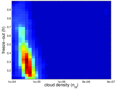
(a)

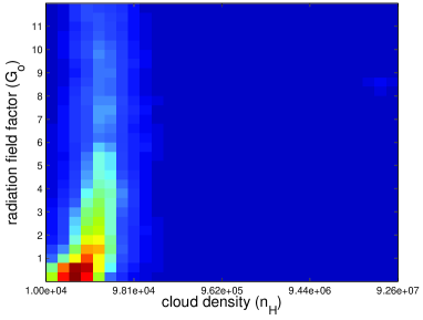
(b)

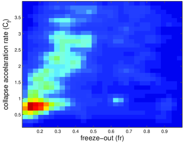
(c)

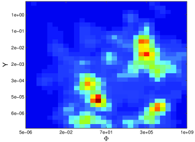
(d)

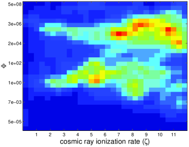
(e)

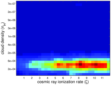
(f)

Figure 4: 2D marginalized posterior probability density functions.Warmer colors indicate higher probability density.

The HDS ratio can be perceived as an index of the level of uncertainty on a predefined definition domain and the higher it is the less constrained is a parameter. Table 4 presents HDS for each parameter for both priors used. Figure 4 shows the 2 dimensional marginal PPD for parameters that present statistical interest. Finally, Table 5 lists the statistical mean and standard deviation for the $\sim 35\%$ HDR of the joint distribution for all the 9 parameter. The general statistical picture we get from Figures 2 and 3 shows that the distributions of all the parameters are far from Gaussian and most of them have more than one modes. Looking at the models with physical units, we can also notice that most of the density lies away from the limits of our definition domain for both cases, which validates our choice for $\mathbb{D}_{{\theta}}$.

3.1 Blind Benchmark Test Results

The results of the performed test as shown in Figure 1 reveal two important insights. First of all, high probability density regions for all the parameters include and hence recover the true parameters. As we can see in Figure 1, all the pre-defined parameter values lie under or very close to the highest density point of the marginal PPD. This result simply validates that both the Bayesian approach makes accurate inference based on the given observations and the MH algorithm samples efficiently the solution space. Secondly, we can observe that in many cases there are additional high probability density regions. These regions prove and highlight the ill-posed nature of our problem by indicating that different parameter sets can produce similar observations. Combining the two insights, we can conclude that the Bayesian method with MCMC sampling is exploring efficiently the parameter space, revealing the solution regions that answer our ill-posed inverse problem. In addition, we can conclude that in order to constrain our solution space we should either introduce numerical regularization factors (e.g. gas phase species) or scientific prior knowledge.

3.2 Influence of priors

A visual comparison of Figures 2 and 3 reveals what we can quantitatively observe in Table 4. With non-informative uniform prior the high density regions seem to cover large sections of the distribution, which in some cases reach $50\%$ of the definition domain. This means that most of the parameters are not constrained enough. The most statistically straightforward parameters seem to be clearly the $n_{H}$ and then the $\phi$ and $fr$ parameters, presenting distinct modes and relatively low HDS. $G_{\circ}$ and $\zeta$ seem neither constrained nor relevant enough, while $fr$ seems to have a clear mode, followed by a very heavy tail. The rest of the parameters present high HDS, above $40\%$ with several disjoint high density regions and do not allow us to reach credible conclusions about the parameters. Including the prior information from the gas phase species changes the picture significantly as can be seen in both Figure 3 and Table 4. We can observe that the HDR get smaller and the parameters seem more constrained. The distribution of $\zeta$ is now denser around high values ($>6$), while $G_{\circ}$ has to be low ($<4$). The $n_{H}$ remains well constrained with even lower HDS, while the distribution of $fr$ now clearly constraints the parameter to low domain values. The distribution of $C_{f}$ is also altered significantly: not only the HDS has dropped, but also a large portion of the density has transfered from high accelerated collapse regions to free fall collapse regions. The non desorption mechanisms still present a multi-modal behavior, but with significantly smaller high density regions. Their distribution clearly highlights the non-linear way these mechanism act together or against each other. For $r$, the addition of informative prior information seems to reduce the HDS as well, centralizing the density, but still favoring slightly the production of H₂O against OH. Therefore, we conclude that the addition of gas phase species as a regularization factor outperforms the use of just a non-informative uniform prior distribution. The HDS is reduced at an average of $\sim 12\%$, which indicates an equivalent constraint on the parameter space. Section 3.3 will discuss the statistical and numerical results of our analysis, while Section 3.4 will discuss the astrophysical implications. For both these Sections we shall only concentrate on the results of the informative prior case.

3.3 High Density Regions

The $n_{H}$ is clearly the most constrained physical parameter. The marginal density function reveals that most of the density is between $2.2$ and $5\times 10^{4}\,cm^{-3}$. The $\zeta$ is constrained to values higher than $6\times 10^{17}\,s^{-1}$, while the $G_{\circ}$ to values lower than $4\>Habing$. The HDR for the $fr$ stays between $20\%$ and $45\%$, while the $C_{f}$ has 1 distinct HDR between $0.5$ and $1.55$ and one long heavy tail between $2$ and $3$ times the default free fall rate. The $\epsilon$ presents two modes. The first HDR is between $0.4$ and $0.8$ and the second between $1.2$ and $1.4$. The marginal distribution of $\phi$, also presents two modes. One is centered around $10^{5}$. The second one is centered around $60$. The marginal distribution for $y$, presents 2 disjoint high density regions as well. The first one indicates really low efficiency of about $10^{-6}$, while the second one a slightly higher $2\times 10^{-3}-8\times 10^{-2}$. Finally, the distribution for the branching ratio parameter $r$ shows high density between $40\%$ and $70\%$ of Oxygen turning into ice water.

In Figure 4 we show the marginalized 2D PPD for our parameters. Note that the $n_{H}$ and the $fr$ are negatively dependent in a nearly linear way. On the other hand $G_{\circ}$ and $n_{H}$ seem to have a non-linear positive correlation, hitting a plateau after a certain gas density. Similarly, the $fr$ and the $C_{f}$ may have a clear peak, but also some evidence of a positive correlation. The relation between the cosmic ray desorption efficiency parameters, $\phi$ and $y$ reveals many distinct peaks throughout the domain space. Note that the marginalized PPD for cosmic ray ionization rate and parameter $\phi$ shows a clear bimodal structure. However, focusing only on the denser areas of the distribution we can observe a potential non linear correlation between the cosmic rays and the efficiency of the cosmic ray related parameter $\phi$. In general though, $\zeta$ is evidently a parameter that is not sufficiently constrained. This is already obvious by the 1D marginal distribution of $\zeta$, but the contrast of constrain between $\zeta$ and one of the most constraint parameters such as $n_{H}$ is depicted in Figure 2(6).

Due to the non-uniqueness of our solution space, examining the joint probability distribution of the PPD provides a useful insight. The dimensionality of the distribution makes a visualization impossible, so we chose to extract the statistical mean and the standard deviation for each one of the parameters from the most probable mode of the joint distribution. The joint distribution was approximated using a multivariate histogram and the most probable mode was chosen in a heuristic way and corresponds to $\sim 35\%$ HDR of the whole PPD. The values for the mean and standard deviation are given in Table 5. As expected, the most probable mode of the joint PPD agrees with the HDR of the marginal parameter distributions. For the unimodal 1D marginalized distributions the most probable mode coincides completely, while for the multi-modal cases the most probable mode coincides with one of the modes. Hence, purely based on the statistical interpretation we conclude that: a molecular cloud that matches the observed abundances should have low $n_{H}$, a low $fr$ and a low $G_{\circ}$. The $\zeta$ on the other hand is more likely to have high values, but the high standard deviation leaves room for significant variation. The collapse of the cloud may be insignificantly accelerated, while the branching ratio $r$ favors slightly the branching into water, but with a high standard deviation. In terms of the non thermal desorption efficiency parameters, we notice increased efficiency for all three of them. As a general result we conclude that the 9D space of the joint distribution has multiple peaks. Both the marginalized distributions and the denser peak of the joint distribution indicate that some of the parameters ($n_{H}$, $G_{\circ},fr,C_{f}$) are well constrained, while other parameters($\zeta,r,\epsilon,\phi,y$) present possible variation that implies further astrophysical or statistical implications.

3.4 Astrophysical Consequences

Here, we discuss our results for each of the parameters with regards to their astrophysical implication:

$\boldsymbol{n_{H}}$: The derived credible intervals for the gas density are in very good agreement with the properties of typical collapsing dark clouds, clumps and cores (Myers & Benson, 1983; Benson & Myers, 1989; Bacmann et al., 2002; Bergin & Tafalla, 2007). Higher cloud densities ($>10^{6}\,cm^{-3}$), that are usually expected in hot cores after the cloud has collapsed (van der Tak, 2004), were explored, but showed nearly zero probability density in our analysis.

$\boldsymbol{fr}$: Our study implies a depletion rate that is not high enough to dominate and is probably lower than $50\%$. Bacmann et al. (2002) suggest that freeze-out dominates when $n_{H}$ exceeds $\sim 3\times 10^{4}\,cm^{-3}$ which is marginally the case in our study. When the freeze out dominates and densities exceed $\sim 10^{5}\,cm^{−3}$ , the abundance of CO ice is found to be significantly increased to typical gaseous values ($\sim 10^{-4}$) (Pontoppidan, 2006; Bergin & Tafalla, 2007). Furthermore, the ice water abundance is typically $5\times 10^{-5}$ to $9\times 10^{-5}$ and even higher at the highest densities (Pontoppidan et al., 2005). The ice CO and H₂O abundances in our case though, are about $0.5-1$ magnitude lower. Therefore, along with the $n_{H}$ results, the lower freeze out rate estimated by our analysis can be explained by a different evolutionary stage of the observed clouds. According to Fontani et al. (2012) low depletion values can also imply a cloud that is going to form less massive objects.

$\boldsymbol{G_{\circ}}$: Our analysis showed that in order to match the observed ice abundances the $G_{\circ}$ is comparable to the standard interstellar radiation field of 1 $Draine$ or $\sim 1.7\,Habing$ (Draine, 1978).

$\boldsymbol{\zeta}$: In dense gas $\zeta$ is measured to be in the range of 1 to $5\times 10^{-17}\,s^{-1}$ (Bergin et al., 1999). However, considerable uncertainties have been reported in the literature with derived values as high as $10^{-15}\,s^{-1}$, accounted to x-rays from a central source (Doty et al., 2004). These discrepancies may be due to whether $\zeta$ is determined via H${}_{3}^{+}$ or HCO⁺ measurements. Yet, Dalgarno (2006) claims that given latest evidence that the $\zeta$ range is narrow and between $10^{-16}$ and $10^{-15}$, the question should be focused not on why the estimations are different, but on why they are so similar. Our analysis confirms $\zeta$ values higher than the typical estimations and is even consistent with the $10^{-16}\,s^{-1}$ estimations through the H${}_{3}^{+}$ determination. Most importantly, our study indicates high standard deviation on these values highlighting that such a variation should be expected. Theoretically, this is explained considering the fact that $\zeta$ lose energy while ionizing and exciting the gas through which they travel in conjunction with the possible variation in the origin of $\zeta$. Even though our astrochemical model does not account for the latter factors, our probabilistic approach reflects their impact.

$\boldsymbol{C_{f}}$: Our study shows that the collapse of the cloud should follow the expected free fall collapse. Higher $C_{f}$ values present moderate probability density, which implies that the observational constraints could potentially also be matched with different but also less likely sets of parameters (e.g. higher values for both $C_{f}$ and $fr$).

$\boldsymbol{\epsilon,\phi,y}$: The desorption from H₂ efficiency parameter ($\epsilon$) estimates are significantly higher than the value reported by Roberts et al. (2007) ($\epsilon<0.1$). The direct cosmic ray desorption efficiency ($\phi$), presents two peak values. One of them agrees with Roberts et al. (2007) and is centered around $10^{5}$. The second one is centered around $60$, which is lower than the lowest limit studied by Roberts et al. (2007). For the cosmic ray-induced photodesorption efficiency ($y$), we have two probable estimates as well. The first one indicates really low efficiency. The second one presents a slightly higher efficiency that is still lower than the one estimated by Hartquist & Williams (1990) ($y=0.1$), but consistent with the results of Öberg et al. (2009) for CO₂. Our analysis in general indicates useful credible intervals for non thermal desorption efficiencies, highlighting though, that the reported non linearities can be tackled with further regularization factors such as molecule specific analysis and additional grain properties. Note as well that our astrochemical model does non include direct UV photodesorption which has recently be found to be efficient.

$\boldsymbol{r}$: The branching ratio proved to be a parameter with high but anticipated variability. Its marginal probability distribution presents the most statistically normal behavior with a mean that implies a shared branching ratio of Oxygen freezing into ice H₂O and ice OH, favoring slightly solid H₂O. The first laboratory experiment to reproduce the ice H₂O formation (Dulieu et al., 2010) implied that the hydrogenation of Oxygen is an important route for water formation. Furthermore, Cazaux et al. (2010) state that species such as OH are only transitory and quickly turn into ice water. However, they also state that $\sim 30\%$ of the O coming on the grain is released in the gas phase as OH which can freeze back as H₂O. A pathway that is included in our model and can explain both the high water abundance on the grains and the shared branching ratio $r$. At last the high branching ratio towards ice OH highlights the importance of ice OH for the production of ice CO₂.

We now look at the correlation between our parameters as presented in Figure 4. The relation between the $n_{H}$ and depletion or freeze out has been the subject of many studies (Bacmann et al., 2002; Christie et al., 2012; Fontani et al., 2012; Hocuk et al., 2014). They all conclude that the amount of depletion, the ice abundances and the density of the cloud should all scale together (Rawlings et al., 1992). Even though our analysis suggests a clear anti-correlation between $n_{H}$ and $fr$ (Figure  4(a)), this result is completely in line with literature, since we are not analyzing the time evolution of the cloud, but instead focus on parameter fitting at specific time points. This negative correlation suggests that the less gas density we have the higher the depletion should be in order to match the observed ice abundances. Our results are also in line with the negative correlation between depletion factor and $n_{H}$, derived by Fontani et al. (2012) from CO observations. The positive correlation between $n_{H}$ and $G_{\circ}$ depicted in Figure 4(b) is confirming that the denser a cloud, the higher $\zeta$ values are needed to match the observations. The plateau after a density value ($\sim 7\times 10^{4}\,cm^{-3}$) indicates that the explored radiation field domain space is not high enough to penetrate the cloud after a density threshold. When $C_{f}$ is increased the freeze out timescale needs to be decreased since the final $n_{H}$ is reached quicker. This reduced timescale requires higher $fr$ values in order to simulate the observed ice abundances and this relation is depicted in Figure 4(c). Even thought not very straightforward, the relation between the cosmic ray desorption efficiency parameters, $\phi$ and $y$, is very interesting (Figure 4(d)). In most cases, the cosmic ray photodesorption efficiency is either low or either high for both direct cosmic ray heating and cosmic ray induced cases. However, there is a significant peak when the direct cosmic ray impact is very efficient, whilst the cosmic ray induced impact is very inefficient.

4 Conclusions

In this paper, we implemented a Bayesian MH parameter estimation analysis to solve a typical ill-posed inverse astrochemical problem. We have employed a chemical modeling code and solid phase observations in order to get a holistic insight into the behavior of physical and chemical parameters that drive ice chemistry in dark molecular clouds. The main conclusions of this work are as follows.

1. The Bayesian method provides a systematic approach to solve nonlinear inverse problems with high noise levels and significant model uncertainties. The MCMC technique allows to sample from complex probability distributions in an efficient way. As highlighted by our Blind Benchmark Test, we can conclude that the latter methods succesfully handle astrochemical ill-posed problems and reveal a more complete set of solution regions. On the contrary, single solution estimates derived from traditional approaches would not have provided a complete picture of the solution space and would have contained a high risk of degeneracy.

2. Our probabilistic approach to physical and chemical parameter estimation used a chemical network with deficiencies (especially for the grain part) and several assumptions. Nevertheless, the results both derived useful credible intervals and highlighted model deficiencies implying even more promising results for tackling physical, chemical and model uncertainties for up to date models with targeted astrophysical goals.

3. We confirm that the joint PPD of the solution space is highly non linear and multimodal and the 1D marginal PPD for each parameter are far from Gaussian highlighting the complexity of the problem.

4. Including abundances of gas phase species as a regularization factor and introduced as a Bayesian prior, increases the parameter constrain efficiency by $12\%$. This result can imply that observational regularization constraints compensate for any chemical code deficiencies. Also, increasing the number of gas phase regularization factors will constrain even more the solution space.

5. We show that physical parameters such as $n_{H}$, $G_{\circ}$, $C_{f}$ are highly constrained and their variation has a great impact on the derived ice abundances.

6. The high variation of $\zeta$ contradicts the theoretical $\zeta$ standard values in dense gas and indicates a larger credible interval instead.

7. Non thermal desorption efficiencies act and counteract in a non linear way with each other or $\zeta$. This complex behavior should be analyzed with extra regularization factors.

8. Branching ratio parameters such as $r$ can be successfully estimated through Bayesian MCMC methods. Our results even though with high variability, indicate that the detail or simplicity of the dust grains chemical network can be encapsulated and reflected as certainty or uncertainty respectively.

Appendix A
Markov Chain Monte Carlo

The MCMC framework uses a Markov chain to explore the parameter space and approximate the posterior probability distribution. This chain consist of a series of states $\boldsymbol{\theta}^{(1)},...,\boldsymbol{\theta}^{(t)},...\boldsymbol{\theta}^{(T)}$, where the probability of $\boldsymbol{\theta}^{(t)}$ depends only on $\boldsymbol{\theta}^{(t-1)}$. MCMC methods require an algorithm for choosing states in the Markov chain in a random way. The MCMC sampler implemented for this paper was the Metropolis-Hastings (MH) algorithm. The MH is briefly outlined here using the following pseudocode:

1. Select a starting point $\boldsymbol{\theta}^{(1)}$ from the parameter space. Then for $i=2,3,...$ until convergence, repeat the following steps.

2. Propose a random set of parameters according to a proposal distribution $q$, so that $\boldsymbol{\theta}^{*}\sim q(\boldsymbol{\theta}^{i}|\boldsymbol{\theta}^{i-1})$

3. Calculate the posterior probability of the new parameters, $\pi(\boldsymbol{\theta}^{*}|\boldsymbol{\mathcal{Y}})$, using equation 2

4. Accept the new parameters with probability

   $$\alpha(\theta^{*}|\theta^{i-1})=min\{1,\frac{q(\theta^{i-1}|\theta^{*})\pi(\theta^{*}|\mathcal{Y})}{q(\theta^{*}|\theta^{i-1})\pi(\theta^{i-1}|\mathcal{Y})}\}$$

5. Calculate $u\sim Uniform(u;0,1)$

6. if $u<a$ then accept the proposal, $\theta^{i}\leftarrow\theta^{*}$; otherwise, reject the proposal and $\theta^{i}\leftarrow\theta^{i-1}$

The performance of the MH algorithm is highly dependent on the proposal distribution. The appropriate distribution should account for the complexity of the target distribution but it should still be computationally easy to draw samples from. In nonlinear problems such as ours, we expect a multimodal non Gaussian target joint distribution. Non gaussianity is not a problem for MCMC algorithms. However classical choices for the proposal distribution (i.e. Gaussian distribution) can potentially prevent the MCMC to converge to the target distribution, since the transition of the chain from one mode to another is not very possible. In our specific case, following former similar choices (eg. Andrieu & Doucet (1999); Bazot et al. (2012)), and taking into account the characteristics of the expected target distribution, we chose the proposal distribution $q(\boldsymbol{\theta}^{*}|\boldsymbol{\theta}^{t})$ to be a mixture of two Gaussians distribution centered at $\boldsymbol{\theta}^{(t)}$ and a uniform distribution on $\mathcal{D}_{{\theta}}$. Hence, for all parameters $\theta^{*}_{k}$ for k=1,..,9

$$\boldsymbol{\theta}^{*} \sim\mathcal{N}_{\mathcal{D}_{\theta}}(\theta^{t}_{k},\sigma^{2}_{k,1})\text{with probability }40\%$$

$$\boldsymbol{\theta}^{*} \sim\mathcal{N}_{\mathcal{D}_{\theta}}(\theta^{t}_{k},\sigma^{2}_{k,2})\text{with probability }40\%$$

$$\boldsymbol{\theta}^{*} \sim\mathcal{U}_{\mathcal{D}_{\theta}}\text{with probability }20\%$$

The values for $\sigma^{2}_{k,1}$ and $\sigma^{2}_{k,2}$ were selected based on test runs. We run $m=8$ independent Markov chains of length $T=200000$. By using parallel and independent chains it is easier to understand the dependence of the MH performance on the initial parameter values guesses. Moreover, parallel chains provide insight on whether convergence has been reached. Convergence was also decided based on empirical graphical aid. The length T of the chains was chosen confidently larger than the value of decided convergence. In our case $q(\cdot)$ will be a symmetrical distribution. That means that $q(\boldsymbol{\theta}^{(t)}|\boldsymbol{\theta}^{*})=q(\boldsymbol{\theta}^{*}|\boldsymbol{\theta}^{(t)})$ and the ratio in the acceptance probability $\alpha$ is simply the PPD ratio computed at $\boldsymbol{\theta}^{*}$ and $\boldsymbol{\theta}^{t}$. In simple words, that parameters that increase the PPD are always accepted, while parameters that decrease the PPD are randomly accepted based on $\alpha$.

APPENDIX B
UCL_CHEM

In recent years the molecular complexity of star forming regions has led in the development of complex, multi-point time dependent, gas-grain chemical and photon-dominated models which more accurately simulate the physics and the chemistry of the observed interstellar material. The chemical modeling code used in this paper is the UCL_CHEM chemical code. A thorough description is given by Viti et al. (2004). UCL_CHEM is a time and depth dependent gas-grain chemical model that can be used to estimate the fractional abundances (with respect to hydrogen) of gas and surface species in every environment where molecules are present. The model includes both gas and surface reactions and determines molecular abundances in environments where not only the chemistry changes with time but also local variations in physical conditions lead to variations in chemistry. Regardless of the object that is modeled, the code will always start from the most diffuse state where all the gas is in atomic form and evolve the gas to its final density. Depending on the temperature, atoms and molecules from the gas freeze on to the grains and they hydrogenate where possible. The advantage of this approach is that the ice composition is not assumed but it is derived by a time-dependent computation of the chemical evolution of the gas-dust interaction process. The main categories for the physical and chemical input parameters are the initial elemental abundances, cosmic ray ionization rate ($\zeta$), radiation field strength ($G_{\circ}$), gas density ($n_{H}$), dust grain characteristics, freeze-out (species depletion rate), desorption processes and reaction database. The initial fractional elemental abundances, compared to the total number of hydrogen nuclei, were taken to be $0.14$, $4.0\times 10^{-4}$ , $1.0\times 10^{-4}$, $7.0\times 10^{-5}$, $1.3\times 10^{-7}$, $1.0\times 10^{-7}$ for helium, oxygen, carbon, nitrogen, sulphur and magnesium (Sofia & Meyer, 2001). The gas phase network used by UCL_CHEM is based on the UMIST database (Millar et al., 2000). Our chemical network also includes surface reactions as in Viti et al. (2004). In total we have 208 species and 2391 gas and surface reactions included in our network As an output, the code will compute the fractional abundances of all atomic and molecular species included in the network as a function of time.

APPENDIX C
Exploring the Posterior Probability Density

The MH simulations provide us with the joint parameter PPD. However, because of the high dimensionality of the distribution it is impossible to represent graphically the joint probability density. Therefore, we compute the marginal density for each parameter or for a subset of parameters by integrating the PPD over the rest of the parameters except the ones we are interest in. For example, to obtain the joint marginal distribution of $\boldsymbol{\theta}_{a}=\{d,fr\}$ we integrate over the rest of the parameters $\boldsymbol{\theta}_{b}=\{{\zeta,rad,bc,\epsilon,\phi,y,r}\}$,

$$\pi(\boldsymbol{\theta}_{a}|\boldsymbol{\mathcal{Y}})=\int\pi(\boldsymbol{\theta}_{a},\boldsymbol{\theta}_{b}|\boldsymbol{\mathcal{Y}})d\boldsymbol{\theta}_{b}$$

The marginal probability distributions are visualized either with simple histograms for the case of univariate probabilities or with a bivariate histogram with intensity map for the case of bivariate probabilities.

Traditionally, in order to explore the posterior distribution, typical Bayesian estimates, such as the Posterior Mean are used. However, for multi-modal and/or non Gaussian distributions the extraction of any useful estimator is most of the times meaningless. Instead, it is convenient to decrease the parameter space to High Density Regions (HDR) or credible intervals. HDR computation and graphical representation is explained thoroughly by Hyndman (1996). Following his paper we shortly define HDR as follows:

Let $f(x)$ be the density function of a random variable $X$. Then the $100(1-a)\%$ HDR is the subset $R(f_{a})$ of the sample space of $X$ such that

$$R(f_{a})={x:f(x)\geq f_{a}}$$

where $f_{a}$ is the largest constant such that $Pr(X\in R(f_{a}))\geq 1-a$

The above definition indicates two very important properties. From all the possible regions, HDR occupy the smallest possible volume and every point in the regions has probability density that is larger or equal than every point that doesn’t belong in the regions. HDR are very useful for analyzing and characterizing multi-modal distributions. In such cases, HDR might consist of several regions that are disjoint due to the number of modes. In the context of ice formation mechanisms these high density regions are very useful statistical outcomes of the Bayesian approach. Such regions provide us with a precise quantitative measure of how the ice and gas observations and their uncertainties impact the cloud parameters.

Table 1: Parameter Definition Domain

Parameters $\boldsymbol{\theta}$	Unit	Definition Domain $\mathbb{D}_{{\theta}}$
$\zeta$	$10^{-17}\cdot s^{-1}$	1-10
$G_{\circ}$	$Habing$	1-10
$n_{H}$	$cm^{-3}$	$10^{4}-10^{8}$
$fr$	-	$0-100\%$
$C_{f}$	-	$0.5-3$
$\epsilon$	yield per H2 formed	$0.01-1$
$\phi$	yield per cosmic ray impact	$10^{2}-10^{6}$
$y$	yield per photon	$10^{-3}-10^{2}$
$r$	-	$0-100\%$

Table 2: Observational Constraints (Average Fractional Abundances)

Solid Phase Species					Gas Phase Species
H2O	CH3OH	CO	CO2		NH2	N2H+	HCO+
$7.47\pm 1.81$	$0.23\pm 0.13$	$1.14\pm 0.84$	$1.89\pm 0.79$		$3.10\pm 2.24$	$0.068\pm 0.049$	$0.20\pm 0.01$

Table 3: Blind Benchmark Test

Parameters $\boldsymbol{\theta}$	Unit	Test Value
$\zeta$	$10^{-17}\cdot s^{-1}$	2.4
$G_{\circ}$	$Habing$	2.6
$n_{H}$	$cm^{-3}$	$10^{5}$
$fr$	-	$42\%$
$C_{f}$	-	$1.3$
$\epsilon$	yield per H2 formed	$0.02$
$\phi$	yield per cosmic ray impact	$150$
$y$	yield per photon	$0.1$
$r$	-	$75\%$

Table 4: High Density Spread.The lower the value of HDS the more constraint is a parameter.

Parameters ${\theta}$	High Density Spread HDS(%)
	Non-Informative Prior	Informative Prior
$\zeta$	$48$	$36$
$G_{\circ}$	$46$	$30$
$n_{H}$	$16$	$09$
$fr$	$38$	$28$
$C_{f}$	$45$	$35$
$\epsilon$	$50$	$42$
$\phi$	$33$	$28$
$y$	$38$	$33$
$r$	$43$	$32$

Table 5: Mean and standard deviation for the most probable mode of the Joint Distribution. The mode corresponds to $\sim 35\%$ HDR of the total joint distribution.

Parameters $\boldsymbol{\theta}$	Unit	Mean Value
$\zeta$	$10^{-17}\cdot s^{-1}$	$8.39(\pm 2.8)$
$G_{\circ}$	$Habing$	$1.79(\pm 1.27)$
$n_{H}$	$cm^{-3}$	$4.07(\pm 2.34)\times 10^{4}$
$fr$	-	$31(\pm 21)\%$
$C_{f}$	-	$1.18(\pm 0.9)$
$\epsilon$	yield per H2 formed	$0.52(\pm 0.35)$
$\phi$	yield per cosmic ray impact	$2.78(\pm 1.12)\times 10^{6}$
$y$	yield per photon	$3.35(\pm 2.27)\times 10^{-3}$
$r$	-	$56(\pm 23)\%$

References

- Andrieu & Doucet (1999) Andrieu C., Doucet A., IEEE Transactions on Signal Proceedings, 47, 2667
- Bacmann et al. (2002) Bacmann, A., Lefloch, B., Ceccarelli, C., et al. 2002, A&A, 389, L6
- Bazot et al. (2012) Bazot, M., Bourguignon, S., & Christensen-Dalsgaard, J. 2012, MNRAS, 427, 1847
- Benson & Myers (1989) Benson, P. J., & Myers, P. C. 1989, ApJS, 71, 89
- Bergin et al. (1999) Bergin, E. A., Plume, R., Williams, J. P., & Myers, P. C. 1999, ApJ, 512, 724
- Bergin & Tafalla (2007) Bergin, E. A., & Tafalla, M. 2007, ARA&A, 45, 339
- Boogert et al. (2011) Boogert, A. C. A., Huard, T. L., Cook, A. M., et al. 2011, ApJ, 729, 92
- Caselli et al. (1999) Caselli, P., Walmsley, C. M., Tafalla, M., Dore, L., & Myers, P. C. 1999, ApJ, 523, L165
- Cazaux et al. (2010) Cazaux, S., Cobut, V., Marseille, M., Spaans, M., & Caselli, P. 2010, A&A, 522, A74
- Christensen & Meyer (2000) Christensen, N., & Meyer, R. 2000, arXiv:astro-ph/0006401
- Christie et al. (2012) Christie, H., Viti, S., Yates, J., et al. 2012, MNRAS, 422, 968
- Dalgarno (2006) Dalgarno, A. 2006, Proceedings of the National Academy of Science, 103, 12269
- Draine (1978) Draine, B. T. 1978, ApJS, 36, 595
- Doty et al. (2004) Doty, S. D., Schöier, F. L., & van Dishoeck, E. F. 2004, A&A, 418, 1021
- Dulieu et al. (2010) Dulieu, F., Amiaud, L., Congiu, E., et al. 2010, A&A, 512, A30
- Feroz & Hobson (2008) Feroz, F., & Hobson, M. P. 2008, MNRAS, 384, 449
- Fitzgerald et al. (2007) Fitzgerald, M. P., Kalas, P. G., & Graham, J. R. 2007, ApJ, 670, 557
- Fontani et al. (2012) Fontani, F., Giannetti, A., Beltrán, M. T., et al. 2012, MNRAS, 423, 2342
- Ford (2005) Ford, E. B. 2005, AJ, 129, 1706
- Gilks et al. (1995) W.R. Gilks, S. Richardson, and G.J. Spiegelhalter, Markov Chain Monte Carlo in Practice, Chapman and Hall, 1995
- Hadamard (1902) J. Hadamard, , Princeton University Bulletin, 13:49–52, 1902
- Hartquist & Williams (1990) Hartquist, T. W., & Williams, D. A. 1990, MNRAS, 247, 343
- Hocuk et al. (2014) Hocuk, S., Cazaux, S., & Spaans, M. 2014, MNRAS, 438, L56
- Hyndman (1996) Rob J. Hyndman, The American Statistician, 50(2):pp. 120–126, 1996
- Idier (2008) Jérôme Idier, ISTE Ltd and John Wiley & Sons Inc, avr. 2008
- Isella et al. (2009) Isella, A., Carpenter, J. M., & Sargent, A. I. 2009, ApJ, 701, 260
- Johnstone et al. (2010) Johnstone, D., Rosolowsky, E., Tafalla, M., & Kirk, H. 2010, ApJ, 711, 655
- Lebesgue (1902) Lebesgue, H., L. 1902, Intégrale, longueur, aire. Université de Paris
- Millar et al. (2000) Millar, T. J., Farquhar, P. R. A., & Willacy, K. 2000, VizieR Online Data Catalog, 412, 10139
- Myers & Benson (1983) Myers, P. C., & Benson, P. J. 1983, Rev. Mexicana Astron. Astrofis., 7, 238
- Öberg et al. (2009) Öberg, K. I., van Dishoeck, E. F., & Linnartz, H. 2009, A&A, 496, 281
- Öberg et al. (2011) Öberg, K. I., Boogert, A. C. A., Pontoppidan, K. M., et al. 2011, IAU Symposium, 280, 65
- Öberg et al. (2011) Öberg, K. I., Boogert, A. C. A., Pontoppidan, K. M., et al. 2011, ApJ, 740, 109
- Pontoppidan et al. (2005) Pontoppidan, K. M., van Dishoeck, E. F., Dartois, E., et al. 2005, Astrochemistry: Recent Successes and Current Challenges, 231, 319
- Pontoppidan (2006) Pontoppidan, K. M. 2006, A&A, 453, L47
- Rawlings et al. (1992) Rawlings, J. M. C., Hartquist, T. W., Menten, K. M., & Williams, D. A. 1992, MNRAS, 255, 471
- Roberts et al. (2007) Roberts, J. F., Rawlings, J. M. C., Viti, S., & Williams, D. A. 2007, MNRAS, 382, 733
- Schöier et al. (2002) Schöier, F. L., Jørgensen, J. K., van Dishoeck, E. F., & Blake, G. A. 2002, A&A, 390, 1001
- Sofia & Meyer (2001) Sofia, U. J., & Meyer, D. M. 2001, ApJ, 554, L221
- van der Tak (2004) van der Tak, F. F. S. 2004, Star Formation at High Angular Resolution, 221, 59
- Viti et al. (2004) Viti, S., Collings, M. P., Dever, J. W., McCoustra, M. R. S., & Williams, D. A. 2004, MNRAS, 354, 1141
- Whittet et al. (2011) Whittet, D. C. B., Cook, A. M., Herbst, E., Chiar, J. E., & Shenoy, S. S. 2011, ApJ, 742, 28