Density Matrix Spectra and Order Parameters in the 1D Extended Hubbard Model

Abstract

Without any knowledge of the symmetry existing in the system, we derive the exact forms of the order parameters which show long-range correlation in the ground state of the one-dimensional extended Hubbard model using a quantum information approach. Our work demonstrates that the quantum information approach can help us to find the explicit form of the order parameter, which cannot be derived systematically via traditional methods in the condensed matter theory.

I Introduction

In many-body physics, the correlation function plays a fundamental role. Especially in theoretical studies, the understanding on many physical phenomena are based on the calculation of the corresponding correlation functionsMahan ; Sachdev . For instance, to investigate the magnetic properties of a system, people often calculate the spin-spin correlation function to learn the possible magnetic order. In 1D case, the system has a ferromagnetic order if the $0$ mode is dominant, and an anti-ferromagnetic order if the $\pi$ mode is dominant. The long-range behavior of the correlation function is associated with the symmetry-breaking in the system, which is an important concept in the understanding of continuous phase transitions. That is, for a certain operator, its non-vanishing value at a long distance denotes a symmetry-broken phase which usually occurs in the thermodynamic limit. Mathematically, if the correlation function

$$C(0,r)=\left\langle O_{0}O_{r}\right\rangle-\left\langle O_{0}\right\rangle\left\langle O_{r}\right\rangle$$ (1)

is a constant in the infinite $r$ limit, we say that the state has a long-range order. The operator $O$ can then be taken as the order parameter to describe the corresponding phase.

Traditionally, to find an appropriate order parameter for a certain phase, people often resort to other methods such as group theory and the renormalization group analysis. Nevertheless, these methods cannot always help us to find the correct form of the order parameter. Hence a method to derive the order parameter systematically is very instructive. Using the variational approach, Furukawa et alDriveOrder proposed a scheme to derive the order parameter. While the scheme is promising, it still needs the knowledge of the degenerated states that lead to the symmetry breaking in the thermodynamic limit. Instead, we proposed recently a scheme to derive the order parameter from the spectrum of the reduced density matrix of the ground state directly COrder . Differ from Furukawa’s scheme, our approach is not variational, and needs only the knowledge of the ground state.

In this paper, we apply the scheme, for the first time, to a realistic model. To start with, we will first demonstrate the derivation of the order parameter in the Hubbard model in section II.1. Then, we apply our scheme to the extended Hubbard model (EHM) in section II.2 and II.3. We show that even without any knowledge of the symmetry of the system, we can derive the exact forms of the order parameters which show long-range correlations in the ground state of the model. A summary would be given in section III.

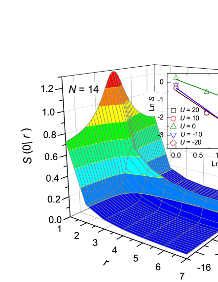
Figure 1: (color online) The mutual information as a function of $r=|i-j|$ and $U$ in the Hubbard model. The inset shows that the mutual information decays algebraically with $r$ and thus long-range correlation is presented in the system.

II Deriving the order parameters

The Hubbard type models has been served as a prototype in condensed matter physics to study the electron correlation effect in solids. Especially in many cases where the long-range Coulomb interaction has significant importance, like in quasi one-dimensional organic solids such as conjugated polymers AP1 and charge transfer crystals AP2 , the extended Hubbard model in one-dimension is the simplest model that included finite range interactions for theoretical studies. The model’s Hamiltonian reads

$$H = -t\sum_{\sigma,j}\left(c_{j,\sigma}^{\dagger}c_{j+1,\sigma}+h.c.\right)$$ (2)

$$+U\sum_{j}n_{j,\uparrow}n_{j,\downarrow}+V\sum_{j}n_{j}n_{j+1},$$

where $c_{j,\sigma}^{\dagger}$ and $c_{j,\sigma}$ ($\sigma=\uparrow,\downarrow$) are creation and annihilation operators of electrons with a spin $\sigma$ at the site $j$ respectively, $n_{j,\sigma}=c_{j,\sigma}^{\dagger}c_{j,\sigma}$, and $n_{j}=n_{j,\uparrow}+n_{j,\downarrow}$. $U$ and $V$ is the strength of the on-site and the nearest-neighbor Coulomb interaction respectively. $t$ is the hoping integral and is taken to be unity for convenience.

Interestingly, the EHM exhibits a very rich phase diagram. It was shown analytically T1 ; T2 ; T3 ; T4 and numerically N1 ; N2 the existence of spin-density waves (SDW), charge-density waves (CDW), phase separation (PS), singlet superconducting (SS) and the triplet superconducting (TS) phases in the model. Using concepts from quantum information theory as a tool, it is also shown that the local entanglement EHM was able to obtain the CDW, SDW and PS phases. In addition to these three phases, the block-block entanglement can also witness the SS phase Deng . Besides the phases mentioned above, there are also studies pointed out the existence of the bond-order waves phase(BOW) in the model. However, whether this BOW exists as a narrow region or just a line in the ground state phase diagram is still a controversial problem BOW ; Jeckelmann ; Jeckelmann2 .

At this point, let us first forget about the result from previous studies and suppose we know nothing about the nature of the phases. To find the potential order existing in the ground state of the model, we need to first examine if the ground state exist a long-range correlation or not. While we do not know the form of any order parameters, we can still use the mutual information, a concept borrowed from quantum information science, to measure the total correlation between two arbitrary blocks in the system. The mutual information is defined as

$$S(i|j)=S\left({\rho}_{i}\right)+S\left({\rho}_{j}\right)-S\left({\rho}_{i\cup j}\right),$$ (3)

where $S\left({\rho}_{i}\right)=-$tr$({\rho}_{i}\log_{2}{\rho}_{i})$ is the von-Neumann entropy of the block $i$. $\rho_{i}$ is the reduced density matrix obtain by tracing out all other degrees of freedom except that of site $i$, i.e.${\rho}_{i}=$tr$\left|\Psi_{0}\right\rangle\left\langle\Psi_{0}\right|$ where $\left|\Psi_{0}\right\rangle$ is the ground state of the system. It has been shown that the existence of the long-range order means that there is a non-vanishing mutual information at a long distance MMWolf ; SJGuJPA . This statement still holds true vice versa. By studying the spectra of the reduced density matrices, we can derive the potential order parameters.

II.1 Case I: $V=0$

To illustrate the scheme more explicitly, let us first ignore the next-nearest neighbor interaction, i.e. $V=0$, and the model is reduced to the conventional Hubbard model Hubbdard ; Gutzwiller ; Kanamori .

Consider a block consists of one site, i.e. $N_{B}=1$. In the basis of local states $\{\left|\mu\right\rangle\}=\{\left|0\right\rangle,\left|\uparrow\right\rangle,\left|\downarrow\right\rangle,\left|\uparrow\downarrow\right\rangle\}$, ${\rho}_{i}$ is found to be diagonal, i.e.

$$\rho_{i}=u\left|0\right\rangle\left\langle 0\right|+v\left|\downarrow\right\rangle\left\langle\downarrow\right|+v\left|\uparrow\right\rangle\left\langle\uparrow\right|+u\left|\uparrow\downarrow\right\rangle\left\langle\uparrow\downarrow\right|,$$ (4)

where $u$ and $v$ are some positive real numbers. The two-site reduced density matrix ${\rho}_{i\cup j}$ is a block-diagonal matrix in the basis $\{\left|\mu\nu\right\rangle\}=\{\left|0\right\rangle,\left|\uparrow\right\rangle,\left|\downarrow\right\rangle,\left|\uparrow\downarrow\right\rangle\}\otimes\{\left|0\right\rangle,\left|\uparrow\right\rangle,\left|\downarrow\right\rangle,\left|\uparrow\downarrow\right\rangle\}$. Figure 1 shows the dependence of the mutual information $S(0|r)$ as a function of $r=|i-j|$ and $U$ calculated for a 14-site system with 7 spin-up electrons and 7 spin-down electrons. The results are obtained from numerical exact diagonalization under periodic boundary conditions. From the figure, we can see that the mutual information reaches a maximum at $U=0$, which is a non-trivial point of the Hubbard model. We will return to this phenomenon later. At this stage we are more interested in the long-range behavior of the mutual information. For this purpose, we plot the dependence of $S(0|r)$ on $r$ in the inset of Figure 1 for various $U$. From the inset, it is easy to find that $S(0|r)$ decays algebraically with $r$. Therefore, we judge that in the ground state of the 1D Hubbard model, there must exist certain kind of long-range correlation though we do not know the explicit form of the order parameter yet.

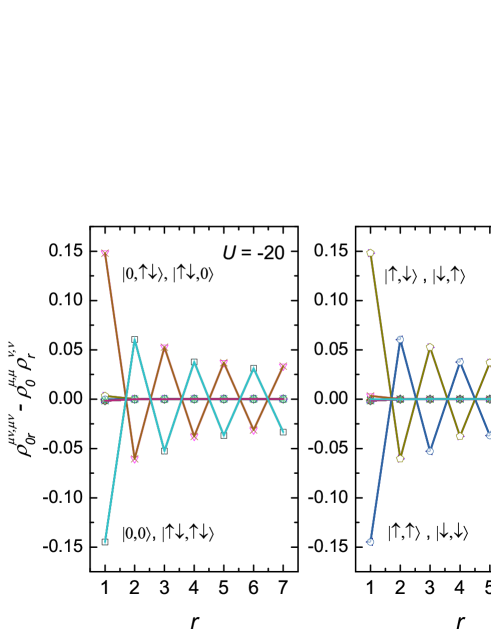
Figure 2: (color online) A plot of $\rho_{0r}^{\mu\nu,\mu\nu}-\rho_{0}^{\mu,\mu}\rho_{r}^{\nu,\nu}$ as a function of $r$ for two limiting cases of $U=-20,20$ in the Hubbard model. For $U=-20$ (left), the charge degrees of freedom ($\{\mu,\nu\}\in\{\left|0\right\rangle,\left|\uparrow\downarrow\right\rangle\}$) are correlated, while for $U=20$(right) the spin degrees of freedom($\{\mu,\nu\}\in\{\left|\uparrow\right\rangle,\left|\downarrow\right\rangle\}$) are correlated.

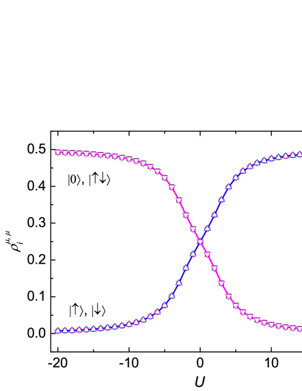
Figure 3: (color online) The diagonal matrix elements, which is also the eigenvalues, of $\rho_{i}$ as a function of $U$ in the Hubbard model. Here $N=14$ and $N_{B}=1$. For the negative $U$ case, the eigenstates $|0\rangle$ and $|\uparrow\downarrow\rangle$ have dominate weights while for positive $U$, the eigenstates $|\uparrow\rangle$ and $|\downarrow\rangle$ have dominate weights.

Diagonal order parameter: According to the scheme we proposed recentlyCOrder , the order parameter can be constructed from the spectrum of the reduced density matrix $\rho_{i}$. However, in most of the cases, we cannot obtain results of the total correlation between two blocks separated by a large enough distance due to the limitation of computational powers.

To single out the correlated elements in $\rho_{i}$, we calculated the difference between the diagonal matrix elements of $\rho_{i\cup j}$ and that of $\rho_{i}\otimes\rho_{j}$ as a function of the separation $|i-j|$. Figure 2 shows a plot of $\rho_{0r}^{\mu\nu,\mu\nu}-\rho_{0}^{\mu,\mu}\rho_{r}^{\nu,\nu}$ as a function of $r$. For convenience, the two block reduced density matrix $\rho_{0\cup r}$ is written as $\rho_{0r}$. From the figure, clearly we can see that $\rho_{0r}\neq\rho_{0}\otimes\rho_{r}$ which is consistence with $S(0|r)\neq 0$. Moreover, for $U=-20$, the difference in the diagonal matrix elements for $\{\mu,\nu\}\in\{\left|0\right\rangle,\left|\uparrow\downarrow\right\rangle\}$ decays algebraically with $r$ while it is almost zero for the others. We can then argue that the vacant state and the double occupancy state of the two blocks are correlated in this case. For the case of $U=20$, $\rho_{0r}^{\mu\nu,\mu\nu}-\rho_{0}^{\mu,\mu}\rho_{r}^{\nu,\nu}$ are almost zero unless $\{\mu,\nu\}\in\{\left|\uparrow\right\rangle,\left|\downarrow\right\rangle\}$. In this limit, the spin up and spin down states are correlated.

In Figure 3, we show the dependence of the eigenvalues of $\rho_{i}$ on the interaction $U$. From the figure, we can see that if $U$ becomes larger and larger, the eigenvalues of the state $\left|\downarrow\right\rangle$ and $\left|\uparrow\right\rangle$ tend to 1/2 and the eigenvalues of $\left|0\right\rangle$ and $\left|\uparrow\downarrow\right\rangle$ vanish. The observation means that in the large $U$ limit, the reduced density matrix becomes

$$\rho_{i}=\frac{1}{2}\left|\downarrow\right\rangle\left\langle\downarrow\right|+\frac{1}{2}\left|\uparrow\right\rangle\left\langle\uparrow\right|.$$ (5)

In the basis of $\rho_{i}\otimes\rho_{j}$, we show the non-zero diagonal and off-diagonal elements of ${\rho}_{i\cup j}$ in Figure 4 and Figure 5 respectively. From the figures, we find that $\rho_{0r}$ takes the form

$$\rho_{0r}=\left(\begin{array}[]{cccc}u&0&0&0\\ 0&v&z&0\\ 0&z&v&0\\ 0&0&0&u\end{array}\right)$$ (6)

in the large $U$ limit in the basis of $\{\left|\uparrow\right\rangle\left|\uparrow\right\rangle,\left|\downarrow\right\rangle\left|\uparrow\right\rangle,\left|\uparrow\right\rangle\left|\downarrow\right\rangle,\left|\downarrow\right\rangle\left|\downarrow\right\rangle\}$. Therefore, the order parameter can be written as

$$O^{d}_{i}=w_{1}\left|\uparrow\right\rangle\left\langle\uparrow\right|+w_{2}\left|\downarrow\right\rangle\left\langle\downarrow\right|.$$ (7)

According to the traceless condition tr$(O_{i}^{d}\rho_{i})=0$, we have $w_{1}=-w_{2}$. Let $w_{1}=1$, then the order parameter becomes

$$O_{i}^{d}=\left|\uparrow\right\rangle\left\langle\uparrow\right|-\left|\downarrow\right\rangle\left\langle\downarrow\right|.$$ (8)

For simplicity, we denote it as $\sigma_{i}^{z}$.

Similarly, for the case of negative $U$, we can find that

$$\rho_{i}=\frac{1}{2}\left|0\right\rangle\left\langle 0\right|+\frac{1}{2}\left|\downarrow\uparrow\right\rangle\left\langle\downarrow\uparrow\right|.$$ (9)

and

$$\rho_{0r}=\left(\begin{array}[]{cccc}u&0&0&0\\ 0&v&z&0\\ 0&z&v&0\\ 0&0&0&u\end{array}\right)$$ (10)

in the basis of $\{\left|0\right\rangle\left|0\right\rangle,\left|0\right\rangle\left|\downarrow\uparrow\right\rangle,\left|\downarrow\uparrow\right\rangle\left|0\right\rangle,\left|\downarrow\uparrow\right\rangle\left|\downarrow\uparrow\right\rangle\}$. Then the diagonal order parameter can be defined as

$$O_{i}^{d}=w_{1}\left|0\right\rangle\left\langle 0\right|+w_{2}\left|\downarrow\uparrow\right\rangle\left\langle\downarrow\uparrow\right|.$$ (11)

Apply the traceless condition and cut-off condition, we get

$$O_{i}^{d}=\left|0\right\rangle\left\langle 0\right|-\left|\downarrow\uparrow\right\rangle\left\langle\downarrow\uparrow\right|.$$ (12)

For simplicity, we denote it as $\eta_{i}^{z}$.

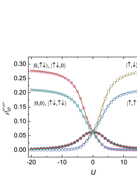
Figure 4: (color online) The diagonal elements of $\rho_{ij}$ as a function of $U$ in the Hubbard model for $r=|i-j|=7$. In the negative $U$ limit, only the matrix elements corresponds to the basis $\{\mu,\nu\}\in\{|0\rangle,|\uparrow\downarrow\rangle\}$ is non-vanishing. In the positive $U$ limit, only the matrix elements corresponds to the basis $\{\mu,\nu\}\in\{|\uparrow\rangle,|\downarrow\rangle\}$ is non-vanishing.

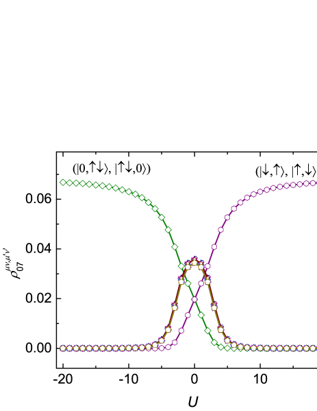
Figure 5: (color online) The non-zero off-diagonal elements of $\rho_{ij}$ as a function of $U$ in the Hubbard model for $r=7$. The matrix elements for $(\mu\nu,\mu^{\prime}\nu^{\prime})$ is the same as $(\mu^{\prime}\nu^{\prime},\mu,\nu)$.

Off-diagonal order parameter: From Eq. (6), we find that $\rho_{0r}$ is not a diagonal matrix. This observation means that there exists off-diagonal long-range correlations in the ground state of the 1D Hubbard model. According to our scheme, the off-diagonal order parameter can be defined as

$$O_{i}^{o}=w\left|\uparrow\right\rangle\left\langle\downarrow\right|+w^{\ast}\left|\downarrow\right\rangle\left\langle\uparrow\right|.$$

Here $w$ is complex, so there are two independent parameters in the operator. We separate the real part and the imaginary part in the operator

$$O_{i}^{o} = x\left(\left|\uparrow\right\rangle\left\langle\downarrow\right|+\left|\downarrow\right\rangle\left\langle\uparrow\right|\right)+iy\left(\left|\uparrow\right\rangle\left\langle\downarrow\right|-\left|\downarrow\right\rangle\left\langle\uparrow\right|\right)$$ (13)

$$= xO_{i}^{x}-yO_{i}^{y}.$$

with

$$O_{i}^{x} = \left|\uparrow\right\rangle\left\langle\downarrow\right|+\left|\downarrow\right\rangle\left\langle\uparrow\right|,$$

$$O_{i}^{y} = -i(\left|\uparrow\right\rangle\left\langle\downarrow\right|-\left|\downarrow\right\rangle\left\langle\uparrow\right|).$$

Obviously, we have

$$\left\langle O_{i}^{x}\right\rangle=\left\langle O_{i}^{y}\right\rangle=0,$$ (14)

and

$$\left\langle O_{i}^{x}O_{j}^{x}\right\rangle=\left\langle O_{i}^{y}O_{j}^{y}\right\rangle=2z.$$ (15)

So we can treat either $O_{i}^{x}$ or $O_{i}^{y}$ or their linear combination as the off-diagonal order operator. Let’s denote them as $\sigma_{i}^{x}$ and $\sigma_{i}^{y}$ respectively.

Similarly, in the negative $U$ region, we can also derive the off-diagonal order parameter as

$$O_{i}^{x} = \left|0\right\rangle\left\langle\uparrow\downarrow\right|+\left|\uparrow\downarrow\right\rangle\left\langle 0\right|,$$

$$O_{i}^{y} = -i(\left|0\right\rangle\left\langle\uparrow\downarrow\right|-\left|\uparrow\downarrow\right\rangle\left\langle 0\right|).$$

We denote them as $\eta_{i}^{x}$ and $\eta_{i}^{y}$ respectively.

$SU(2)$ algebra and the effective Hamiltonian: In the basis of $\{\left|\uparrow\right\rangle,\left|\downarrow\right\rangle\}$, $\sigma_{i}^{x},\sigma_{i}^{y}$ and $\sigma_{i}^{z}$ can be written as

$$\sigma_{i}^{x}=\left(\begin{array}[]{cc}0&1\\ 1&0\end{array}\right),\sigma_{i}^{y}=\left(\begin{array}[]{cc}0&-i\\ i&0\end{array}\right);\sigma_{i}^{z}=\left(\begin{array}[]{cc}1&0\\ 0&-1\end{array}\right).$$ (16)

These expressions are exactly the form the Pauli matraces, which satisfy the su(2) Lie algebra, i.e. $[\sigma_{i}^{\alpha},\sigma_{j}^{\beta}]=2i\delta_{ij}\epsilon^{\alpha\beta\gamma}\sigma_{i}^{\gamma}$. As we know, in the large $U$ limit, the Hubbard model becomes the one-dimensional Heisenberg model

$$H=J\sum_{j}\mathbf{S}_{j}\cdot\mathbf{S}_{j+1},$$

where $J=4t^{2}/U$. In the ground state of the Heisenberg model, the spin-spin correlation has a power-law decaying behavior. The order parameters derived is consistent with our knowledge.

On the other hand, in the negative $U$ region, $\eta_{i}^{x}$, $\eta_{i}^{y}$, and $\eta_{i}^{z}$ can be written as

$$\eta_{i}^{x}=\left(\begin{array}[]{cc}0&1\\ 1&0\end{array}\right),\eta_{i}^{y}=\left(\begin{array}[]{cc}0&-i\\ i&0\end{array}\right);\eta_{i}^{z}=\left(\begin{array}[]{cc}1&0\\ 0&-1\end{array}\right)$$ (17)

in the basis of $\{\left|0\right\rangle,\left|\uparrow\downarrow\right\rangle\}$. Clearly the three operators satisfy the su(2) Lie algebra too.

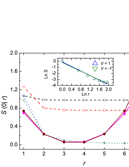
Figure 6: (color online) The mutual information as a function of $r=|i-j|$ for $U=6$ in EHM. The inset shows a ln-ln plot of the mutual information versus $r$ for $V=\pm 1$.

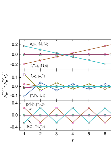
Figure 7: (color online) A plot of $\rho_{0r}^{\mu\nu,\mu\nu}-\rho_{0}^{\mu,\mu}\rho_{r}^{\nu,\nu}$ as a function of $r$ for $V=-8$ (top panel), $V=1$ (middle panel), and $V=8$ (bottom panel) in EHM for $U=6$. For $V=\pm 8$, the charge degrees of freedom ($\{\mu,\nu\}\in\{\left|0\right\rangle,\left|\uparrow\downarrow\right\rangle\}$) are correlated, while for $V=1$ the spin degrees of freedom($\{\mu,\nu\}\in\{\left|\uparrow\right\rangle,\left|\downarrow\right\rangle\}$) are correlated.

II.2 Case II: $V\neq 0$, $U=6$

Now, let us also include the next-nearest neighbor interaction in the system. Figure 6 shows a plot of the mutual information as a function of $r$. Obviously, the mutual information is non-vanishing at a large $r$ for $V=\pm 4,\pm 8$ (in fact, they corresponds to two different regime where $V>U/2$ and $V<-U/2$ which we will see more explicitly later). For the intermediate case, we can see from the log-log plot in the inset that the mutual information shows a power law decaying behavior. One can then safely argue that the system exhibits certain kind of long-range correlations and we can go on to investigate the spectrum of the reduce density matrix to derive the potential order parameters.

Using the same basis as that for the Hubbard model in the previous subsection, we calculated the single-site and two-sites reduced density matrices. $\rho_{i}$ is diagonal and takes the form of Eq. 4. Figure 7 shows a plot of the difference between the diagonal matrix element of $\rho_{0r}$ and the product of the diagonal matrix elements of $\rho_{0}$ and $\rho_{r}$ with the corresponding basis as a function of $r$. The finite difference in $\rho_{0r}^{\mu\nu,\mu\nu}-\rho_{0}^{\mu,\mu}\rho_{r}^{\nu,\nu}$ for some particular $\mu$ and $\nu$ indicates that $\rho_{0r}\neq\rho_{0}\otimes\rho_{r}$. For $V=-8$ and $V=8$, we see that the main contributors to the correlation of two sites separated at a large distance are the states $|0\rangle$ and $|\uparrow\downarrow\rangle$. While for the case of $V=1$, the $|\uparrow\rangle$ and $|\downarrow\rangle$ states play the role.

Figure 8 plots the eigenvalues of the single-site reduced density matrix as a function of $V$. The crossings of the eigenvalues, which is the probabilistic weight of the corresponding eigenstates, of $\rho_{i}$ separate the system into three different regimes corresponding to $V\lesssim-U/2$, $-U/2\lesssim V<U/2$, and $V>U/2$. This echoes what we have mentioned in the previous paragraph. In each of the regime, the kind of correlation existing in the system is qualitatively different as one can judge from the nature of the dominating eigenstates.

For $-U/2\lesssim V<U/2$, the eigenvalues of the $|\downarrow\rangle$ and $|\uparrow\rangle$ states are around $1/2$ while that are almost zero for the $|0\rangle$ and $|\uparrow\downarrow\rangle$ states. Following similar argument in the previous section, we can define the order parameter as

$$O_{i}=w_{1}|\uparrow\rangle\langle\uparrow|+w_{2}|\downarrow\rangle\langle\downarrow|.$$

Again, by applying the traceless condition and take $w_{1}=1$, we obtain the order parameter

$$O_{i}=|\uparrow\rangle\langle\uparrow|-|\downarrow\rangle\langle\downarrow|=\sigma_{i}^{z}.$$ (18)

For $V\lesssim-U/2$ and $V>U/2$, the eigenvalues corresponds to the states $|0\rangle$ and $\uparrow\downarrow\rangle$ are around one-half while that for the states $|\uparrow\rangle$ and $|\downarrow\rangle$ tends to zero. Note that the discrepancy from the value $1/2$ and $0$ respectively for $V\lesssim-U/2$ is due to the finite size effect. Nevertheless, we show the size dependence of $\rho_{i}^{\mu,\mu}$ for $V=-6$ in the inset of Fig. 8. The eigenvalues for the $|\uparrow\rangle$ and $|\downarrow\rangle$ becomes vanishing as the system size increases. We can define the order parameter as

$$O_{i}=w_{1}|0\rangle\langle 0|+w_{2}|\uparrow\downarrow\rangle\langle\uparrow\downarrow|.$$

The choice of the order parameter can be narrow down by applying the traceless condition and again taking $w_{1}$ to be $1$. We have

$$O_{i}=|0\rangle\langle 0|-|\uparrow\downarrow\rangle\langle\uparrow\downarrow|=\eta_{i}^{z}.$$ (19)

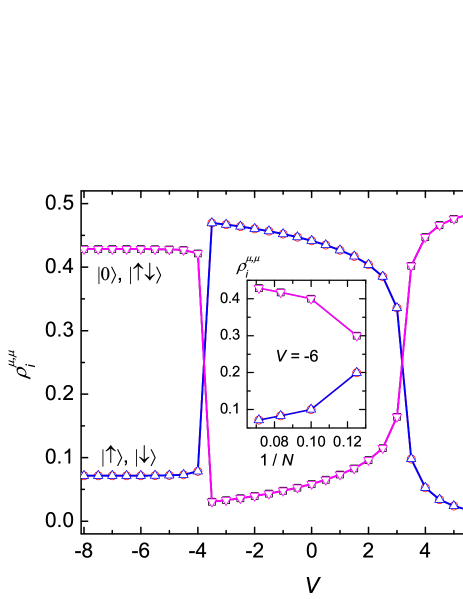
Figure 8: (color online) A plot of the eigenvalues of $\rho_{i}$ as a function of $V$ for $U=6$ in EHM. The inset shows the size dependence of the eigenvalues of $\rho_{i}$ for $V=-6$. For $V\lesssim-U/2$ and $V>U/2$, the eigenstates $|0\rangle$ and $|\uparrow\downarrow\rangle$ have dominate weights. For $-U/2\lesssim V<U/2$, the eigenstates $|\uparrow\rangle$, and $|\downarrow\rangle$ are dominated.

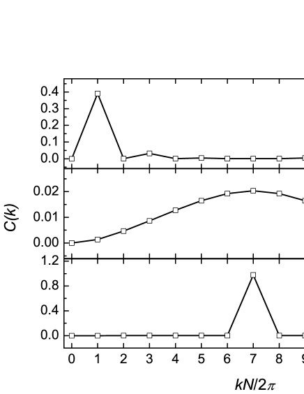
Figure 9: The correlation function calculated from the derived order operators in the momentum space as a function of $k$ in EHM. Here $U=6$, $N=14$, and $V=-8$ (top panel), $V=1$ (middle panel), and $V=8$ (bottom panel) respectively.

Here we obtained the same order parameter for both of the regimes where $V\lesssim-U/2$ and $V>U/2$. However, recall from Fig. 6, the mutual information as a function of $r$ shows qualitatively different behavior in these two range of values of $V$. For $V>U/2$, the mutual information almost remains constant as $r$ increases. On the other hand, for $V\lesssim-U/2$, the mutual information first decreases and then increases to a maximum value upon reaching $r=7$, where it is the middle of the chain. It is reasonable to suspect that the ground state of the system is qualitatively different in these two regimes. To further distinguish between them, it is worth to study the mode of the order parameters.

With the order parameter found in Eq. (19), one can calculate the correlation function in Eq. (1) and it is found to be oscillating with respect to $r$ as expected. To capture the mode of the order parameter, let’s consider the Fourier transformation of the correlation function, i.e.

$$C(k)=\frac{1}{N}\sum_{r=0}^{N-1}e^{-ikr}C(0,r)=\frac{1}{N}\sum_{r=0}^{N-1}e^{-ikr}\langle\eta_{0}^{z}\eta_{r}^{z}\rangle,$$ (20)

where $k=2m\pi/N$ and $m=0,1,\cdots,N-1$. Also note that $\langle\eta_{i}^{z}\rangle=0$ as a result of applying the traceless condition. The result is plotted in Fig. 9.

From the figure, we see that the correlation function peaks at $k=\pi$ for $V=8$. One can expect this holds true for the whole range of $V>U/2$. Together with the form of the derived order parameter, we may conclude that the dominating configuration in the ground state of the system are consisting of alternating vacant and double occupancy states. This is in fact the well-know charge-density wave (CDW) states $|0,\uparrow\downarrow,\cdots,0,\uparrow\downarrow\rangle$ and $|\uparrow\downarrow,0,\cdots,\uparrow\downarrow,0\rangle$ in the extended Hubbard model.

For $V\lesssim-U/2$, the mode of the order parameter are $k=2\pi/N$ and $2\pi(N-1)/N$. The second peak in the correlation function $C(k)$ is just a result from the periodic boundary conditions. In this regime, one can deduce that the dominating ground state configurations has a period of half of the lattice in the real space. They are the phase separation (PS) states $|0,\cdots,0,\uparrow\downarrow,\cdots,\uparrow\downarrow\rangle$ and the translation of it. This also explains why the mutual information is maximum for the sites separated by half of the lattice. Since any of the translation of the above state are equally weighted in the ground state before symmetry is broken, only the local states separated by half of the lattice can be confidently determine once we know one of them. They have to be opposite to each other.

For completeness, we also studied the mode of the order parameter for $-U/2\lesssim V<U/2$. The correlation function

$$C(k)=\frac{1}{N}\sum_{r=0}^{N-1}e^{-ikr}\langle\sigma_{0}^{z}\sigma_{r}^{z}\rangle$$ (21)

as a function of $k$ is shown in the middle panel of Fig. 9. The maximum of the correlation function occurs at $k=\pi$. We can similarly deduce that the dominating configuration are the spin-density wave (SDW) states $|\uparrow,\downarrow,\cdots,\uparrow,\downarrow\rangle$ and $|\downarrow,\uparrow,\cdots,\downarrow,\uparrow\rangle$. These results obtained are consistent with previous studies EHM .

II.3 Case III: $V\neq 0$, $U=4$

Let’s now consider a block size of two sites, i.e. $N_{B}=2$. In the following, we will use $i$ to denote a single-site and $\tilde{i}$ to denote a single-block consist of two neighboring sites. The single-block (two-site) reduced density matrix $\rho_{\tilde{i}}$ is calculated for the case of $U=4$ and $N=14$. In the basis of $\{\left|0\right\rangle,\left|\uparrow\right\rangle,\left|\downarrow\right\rangle,\left|\uparrow\downarrow\right\rangle\}\otimes\{\left|0\right\rangle,\left|\uparrow\right\rangle,\left|\downarrow\right\rangle,\left|\uparrow\downarrow\right\rangle\}$, the eigenstates of $\rho_{\tilde{i}}$ have the form of

$$|\phi_{A}\rangle = |\uparrow\downarrow,\uparrow\downarrow\rangle,$$

$$|\phi_{B}\rangle = |0,0\rangle,$$

$$|\phi_{C}\rangle = \frac{1}{\sqrt{2}}\big{(}|\uparrow\downarrow,\downarrow\rangle+|\downarrow,\uparrow\downarrow\rangle\big{)},$$

$$|\phi_{D}\rangle = \frac{1}{\sqrt{2}}\big{(}|\uparrow,0\rangle-|0,\uparrow\rangle\big{)},$$

$$|\phi_{E}\rangle = \frac{1}{\sqrt{2}}\big{(}|\downarrow,0\rangle-|0,\downarrow\rangle\big{)},$$

$$|\phi_{F}\rangle = \frac{1}{\sqrt{2}}\big{(}|\uparrow\downarrow,\uparrow\rangle+|\uparrow,\uparrow\downarrow\rangle\big{)},$$

$$|\phi_{G}\rangle = \alpha\big{(}|\uparrow\downarrow,0\rangle+|0,\uparrow\downarrow\rangle\big{)}-\beta\big{(}|\uparrow,\downarrow\rangle-|\downarrow,\uparrow\rangle\big{)},$$

$$|\phi_{H}\rangle = \frac{1}{\sqrt{2}}\big{(}|\uparrow,\downarrow\rangle+|\downarrow,\uparrow\rangle\big{)},$$

$$|\phi_{I}\rangle = |\uparrow,\uparrow\rangle,$$

$$|\phi_{J}\rangle = |\downarrow,\downarrow\rangle,$$

$$|\phi_{K}\rangle = \frac{1}{\sqrt{2}}\big{(}|\uparrow\downarrow,\downarrow\rangle-|\downarrow,\uparrow\downarrow\rangle\big{)},$$

$$|\phi_{L}\rangle = \frac{1}{\sqrt{2}}\big{(}|\uparrow,0\rangle+|0,\uparrow\rangle\big{)},$$

$$|\phi_{M}\rangle = \frac{1}{\sqrt{2}}\big{(}|\downarrow,0\rangle+|0,\downarrow\rangle\big{)},$$

$$|\phi_{N}\rangle = \frac{1}{\sqrt{2}}\big{(}|\uparrow\downarrow,\uparrow\rangle-|\uparrow,\uparrow\downarrow\rangle\big{)},$$

$$|\phi_{O}\rangle = \frac{1}{\sqrt{2}}\big{(}|\uparrow\downarrow,0\rangle-|0,\uparrow\downarrow\rangle\big{)},$$

$$|\phi_{P}\rangle = \gamma\big{(}|\uparrow\downarrow,0\rangle+|0,\uparrow\downarrow\rangle\big{)}+\delta\big{(}|\uparrow,\downarrow\rangle-|\downarrow,\uparrow\rangle\big{)},$$ (22)

where $\alpha,\beta,\gamma,\delta$ are positive real numbers.

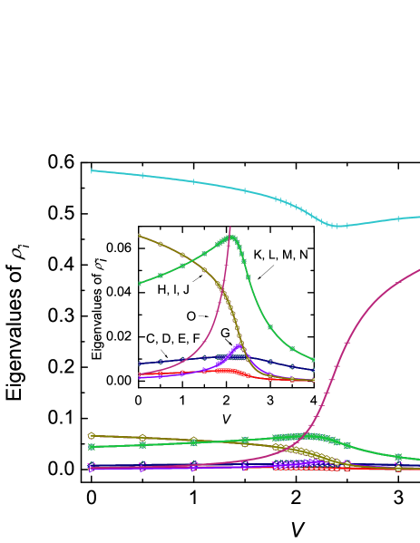
Figure 10: (color online) The eigenvalues of the single-block (two-site) reduced density matrix $\rho_{\tilde{i}}$ as a function of $V$ in the 1D extended Hubbard model. $N=14$ and $U=4$. The inset shows a close-up of the low-lying states.

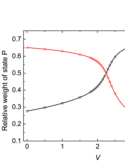
Figure 11: (color online) The relative weight of the $\gamma$ and $\delta$ in the eigenstate $\left|\phi_{P}\right\rangle$ of the single-block reduced density matrix as a function of $V$. $N=14$, $U=4$, and $N_{B}=2$.

Figure 10 shows a plot of the eigenvalues of the corresponding eigenstates as a function of $V$. From the figure, we can see that some of the states, for examples, states $\{\left|\phi_{C}\right\rangle,\left|\phi_{D}\right\rangle,\left|\phi_{E}\right\rangle,\left|\phi_{F}\right\rangle\}$ and states $\{\left|\phi_{K}\right\rangle,\left|\phi_{L}\right\rangle,\left|\phi_{M}\right\rangle,\left|\phi_{N}\right\rangle\}$, are degenerated respectively. The degeneracy tells us that there are spin-up-down and charge symmetries in the system.

Among all the eigenstates, the weight of the state $\left|\phi_{P}\right\rangle$ is dominated for the whole range of value of $V$ shown. This state is a spin-singlet state. It is a superposition of two parts, the charge part $\left|\uparrow\downarrow,0\right\rangle+\left|0,\uparrow\downarrow\right\rangle$ and the spin part $\left|\uparrow,\downarrow\right\rangle+\left|\downarrow,\uparrow\right\rangle$ with relative weight characterized by $\gamma$ and $\delta$ respectively. The magnitude of $\gamma$ and $\delta$ are plotted as a function of $V$ in Fig. 11. There is a crossing between the two magnitudes around $V=2$. For $V>>2$, the relative weight of the charge part is much greater than that of the spin part. Besides, considering the region $V>>2$ in Fig. 10 again, the second dominating state is $\left|\phi_{O}\right\rangle$ which overwhelms all other eigenstates except $\left|\phi_{P}\right\rangle$. From Eq. (22), we also notice that the state $\left|\phi_{O}\right\rangle$ only consists of the charge part. As a result, we may argue that in the this region, the charge part is decoupled from the spin part. The reduced density matrix can be reduced to an effective one in Eq. (10).

Similarly, for $V<<2$, the spin part in $\left|\phi_{P}\right\rangle$ outweigh the charge part as one can realize from Fig. 11. The eigenvalues for $\left|\phi_{H}\right\rangle$, $\left|\phi_{I}\right\rangle$, and $\left|\phi_{J}\right\rangle$ also dominate in the low-lying eigenstates. The spin degree of freedom is singled out in this regime and the reduced density matrix can be effectively expressed as the one in Eq. (6).

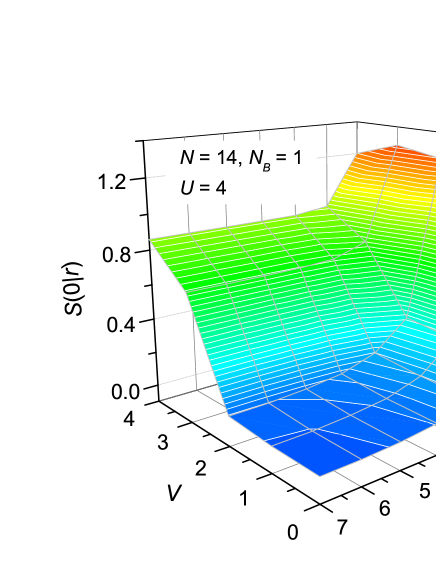
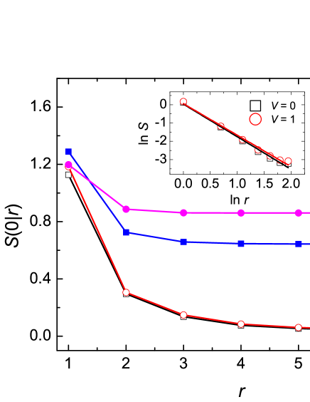
Figure 12: (color online) (Top) A 3D plot of the mutual information between two single sites as a function of $V$ and $r$ in the 1D extended Hubbard model. $N=14$, $U=4$ and $N_{B}=1$. (Bottom) A plot of the mutual information as a function of $r$ for $V=0,1,3,4$. The inset shows a ln-ln plot of the mutual information as a function of $r$ for $V=0,1$.

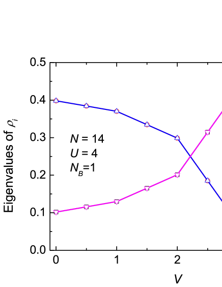
Figure 13: (color online) The eigenvalues of the single-site reduced density matrix as a function of $V$ in the 1D extended Hubbard model. Here $N=14$, $U=4$ and $N_{B}=1$.

In Fig. 12, the mutual information between two single sites are calculated as a function of $V$ and the separation $r$. In the 2D plot, we can see that the mutual information for $V>2$ is non-vanishing at a long distance. For $V<2$, the ln-ln plot in the inset also shows that the mutual information decays algebraically with $r$. So the long-range correlation in the two regimes is already captured by a block size of one site. To construct the order parameter in these regimes, we may go back to consider the single-site reduced density matrix.

Figure 13 is a plot of the eigenvalues of the single-site reduced density matrix. It is qualitatively the same as the case of $U=6$. The $\left|\uparrow\right\rangle$ and $\left|\downarrow\right\rangle$ states are dominated for $V<2$ while the $\left|0\right\rangle$ and $\left|\uparrow\downarrow\right\rangle$ states are dominated for $V>2$. Following similar analysis in the previous sections, we can find that the order operators are $\sigma_{i}^{z}$ and $\eta_{i}^{z}$, which characterize the SDW and CDW respectively, in the two regions.

However, the above is not the whole story. The single-site reduced density matrix was not enough to capture the correlation in the system around $V=2$. Returning to Fig. 10, the eigenvalue of $\left|\phi_{P}\right\rangle$ has a drop around $V=2$ and there is also a relatively large rise in the weight of the eigenstates $\left|\phi_{K}\right\rangle$, $\left|\phi_{L}\right\rangle$, $\left|\phi_{M}\right\rangle$ and $\left|\phi_{N}\right\rangle$. In addition, the magnitude of $\gamma$ and $\delta$ in $\left|\phi_{P}\right\rangle$ becomes comparable in this intermediate value. These observation suggest that the spin part and the charge part are coupled around $V=2$. There may exist some other kind of long-range correlation rather than SDW and CDW in this intermediate region.

Let’s consider $N_{B}=2$ again and rearrange the single-block reduced density matrix from the basis of $\{\left|0\right\rangle,\left|\uparrow\right\rangle,\left|\downarrow\right\rangle,\left|\uparrow\downarrow\right\rangle\}_{i}\otimes\{\left|0\right\rangle,\left|\uparrow\right\rangle,\left|\downarrow\right\rangle,\left|\uparrow\downarrow\right\rangle\}_{i+1}$ to $\{\left|0,0\right\rangle,\left|0,\uparrow\right\rangle,\left|\uparrow,0\right\rangle,\left|\uparrow,\uparrow\right\rangle\}_{\tilde{i}}\otimes\{\left|0,0\right\rangle,\left|0,\downarrow\right\rangle,\left|\downarrow,0\right\rangle,\left|\downarrow,\downarrow\right\rangle\}_{\tilde{i}}$. The purpose of doing this is that we want to filter out the spin-down degree of freedom from the spin-up degree of freedom (or vice versa). After the rearrangement, we traced out the spin-down degree of freedom. The resulting reduced density matrix has the form of

$$\rho_{\tilde{i}\uparrow}=\begin{pmatrix}u&0&0&0\\ 0&v&z&0\\ 0&z&v&0\\ 0&0&0&u\\ \end{pmatrix},$$ (23)

in the basis of $\{\left|0,0\right\rangle,\left|0,\uparrow\right\rangle,\left|\uparrow,0\right\rangle,\left|\uparrow,\uparrow\right\rangle\}_{\tilde{i}}$. Similarly, if we trace out the degree of freedom for spin-up, we have

$$\rho_{\tilde{i}\downarrow}=\begin{pmatrix}u&0&0&0\\ 0&v&z&0\\ 0&z&v&0\\ 0&0&0&u\\ \end{pmatrix},$$ (24)

in the basis of $\{\left|0,0\right\rangle,\left|0,\downarrow\right\rangle,\left|\downarrow,0\right\rangle,\left|\downarrow,\downarrow\right\rangle\}_{\tilde{i}}$.

Next, we would like to compare the off-diagonal matrix elements $z$ in $\rho_{\tilde{i}\uparrow}$ and $\rho_{\tilde{i}\downarrow}$ with that corresponding to SDW and CDW. The weight of SDW is given by the coefficient of $\left|\uparrow,\downarrow\right\rangle\left\langle\uparrow,\downarrow\right|$ or $\left|\downarrow,\uparrow\right\rangle\left\langle\downarrow,\uparrow\right|$ (the notation here is in form of $\left|i,i+1\right\rangle\left\langle i,i+1\right|$). From Eq. (22), it can be obtained by

$$P_{\text{SDW}}=\delta^{2}p_{P}+0.5p_{H}+\beta^{2}p_{G},$$ (25)

where the $p$’s are the eigenvalues of the corresponding eigenstates in Eq. (22). For the weight of CDW, we obtained it by considering the matrix element corresponds to $\left|0,\uparrow\downarrow\right\rangle\left\langle 0,\uparrow\downarrow\right|$ or $\left|\uparrow\downarrow,0\right\rangle\left\langle\uparrow\downarrow,0\right|$ from Eq. (22). We have

$$P_{\text{CDW}}=\gamma^{2}p_{P}+0.5p_{O}+\alpha^{2}p_{G}.$$ (26)

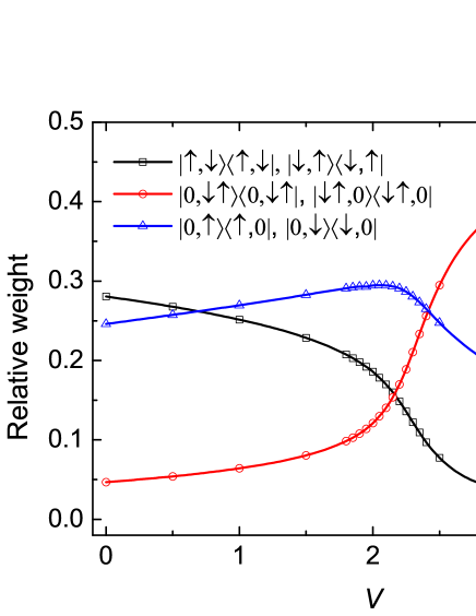
Figure 14: (color online) The relative weight of some of the matrix elements in the single-block reduced density matrix in the 1D extended Hubbard model as a function of $V$. $N=14$, $U=4$ and $N_{B}=2$.

Figure 14 shows a plot of $P_{\text{SDW}}$, $P_{\text{CDW}}$ and $z$ as a function of $V$. On the two sides far away from $V=2$, the largest weight would correspond to SDW and CDW respectively as expected from previous analysis. However, around $V=2$, the off-diagonal matrix element in $\rho_{\tilde{i}\uparrow}$ and $\rho_{\tilde{i}\downarrow}$ are dominating instead. If we just pick this dominating weight to define the order parameter, we have

$$O_{\tilde{i}} = \omega_{1}\left|0,\uparrow\right\rangle\left\langle\uparrow,0\right|+\omega^{*}_{1}\left|\uparrow,0\right\rangle\left\langle 0,\uparrow\right|$$ (27)

$$+\omega_{2}\left|0,\downarrow\right\rangle\left\langle\downarrow,0\right|+\omega^{*}_{2}\left|\downarrow,0\right\rangle\left\langle 0,\downarrow\right|.$$

As mentioned before, the system possess up-down spin symmetry. We could take $\omega_{1}=\omega_{2}=\omega$, and then separate the operator into the real and imaginary part. We have

$$O_{\tilde{i}} = \omega\Big{(}\left|0,\uparrow\right\rangle\left\langle\uparrow,0\right|+\left|0,\downarrow\right\rangle\left\langle\downarrow,0\right|\Big{)}$$ (28)

$$+\omega^{*}\Big{(}\left|\uparrow,0\right\rangle\left\langle 0,\uparrow\right|+\left|\downarrow,0\right\rangle\left\langle 0,\downarrow\right|\Big{)},$$

$$= x\Big{(}\left|0,\uparrow\right\rangle\left\langle\uparrow,0\right|+\left|0,\downarrow\right\rangle\left\langle\downarrow,0\right|$$

$$+\left|\uparrow,0\right\rangle\left\langle 0,\uparrow\right|+\left|\downarrow,0\right\rangle\left\langle 0,\downarrow\right|\Big{)}$$

$$+iy\Big{(}\left|0,\uparrow\right\rangle\left\langle\uparrow,0\right|+\left|0,\downarrow\right\rangle\left\langle\downarrow,0\right|$$

$$-\left|\uparrow,0\right\rangle\left\langle 0,\uparrow\right|-\left|\downarrow,0\right\rangle\left\langle 0,\downarrow\right|\Big{)}.$$

Either the first term or the second term in the bracket above, or their linear combination can be taken as the order parameter. Let’s take the real part as the order parameter, i.e

$$O_{\tilde{i}} = \left|0,\uparrow\right\rangle\left\langle\uparrow,0\right|+\left|0,\downarrow\right\rangle\left\langle\downarrow,0\right|$$ (29)

$$+\left|\uparrow,0\right\rangle\left\langle 0,\uparrow\right|+\left|\downarrow,0\right\rangle\left\langle 0,\downarrow\right|.$$

In terms of the fermion creation and annihilation operators, we have

$$O_{\tilde{i}}=c_{i,\uparrow}^{\dagger}c_{i+1,\uparrow}+c_{i+1,\uparrow}^{\dagger}c_{i,\uparrow}+c_{i,\downarrow}^{\dagger}c_{i+1,\downarrow}+c_{i+1,\downarrow}^{\dagger}c_{i,\downarrow},$$ (30)

which is the conventional order parameter that has been used to investigate the BOW in the extended Hubbard model Zhang2004 .

III summary

We summarize our scheme of constructing the order parameter in the following: (i) Calculate the mutual information to see whether there exists any long-range correlation in the system. Choose the minimum size of the block where the mutual information is non-vanishing for two blocks separated by a large distance. (ii) Calculate the difference between the diagonal matrix elements of the two block reduced density matrix and the product of the diagonal matrix elements of two single block reduced density matrix. This is to single out the correlating elements from other noise due to the finite size effect. (iii) Obtain the eigenvalues and eigenvectors of the single block reduced density matrix. Construct the order parameter from the heavy weighted eigenstates. Apply traceless condition and cut-off condition to narrow down the choice. (iv) Calculate the correlation function using the derived order parameter and study the mode of it.

With the scheme proposed, we have derived the order parameters which show long-range correlation in the ground state of the 1D EHM without using any empirical knowledge. Such an application confirmed that the order parameter for a quantum many-body system can be systematically derived even without the knowledge of symmetry in the system. We expect that our scheme can shed new lights on the controversies in some frustrated antiferromagnetfrustraedSpin and bond-order wave in the extended Hubbard modelBOW ; Jeckelmann ; Jeckelmann2 .

Throughout the paper, the system size being simulated was 14 sites. Remarkably, we see that even for such a small system size, the spectra of the single-site or two-site reduced density matrices were able to capture the information of the nature of the order in the ground state of the system. This may be a promising scheme as one could have insight on the order existing in the system without simulating a large system, which requires intensive computational powers. However, we would like to mention that the crossing of the dominating states in the reduced density matrix spectrum may not locate the phase boundaries exactly. To locate the phase boundaries, one can use the order operator derived to calculate the correlation function and then perform finite size scaling analysis.

This work is supported by the Earmarked Grant Research from the Research Grants Council of HKSAR, China (Project No. CUHK 401213).

References

- (1) G. D. Mahan, Many Particle Physics, (Kluwer Academic/Plenum Publishers, New York, 2000).
- (2) S. Sachdev, Quantum Phase Transitions, (Cambridge University Press, Cambridge, UK, 2000).
- (3) S. Furukawa, G. Misguich, and M. Oshikawa, Phys. Rev. Letts. 96, 047211 (2006).
- (4) S. J. Gu, W. C. Yu, and H. Q. Lin, Ann. Phys., 336, 118 (2013).
- (5) G. W. Hayden and Z. G. Soos, Phys. Rev. B 38, 6075 (1988); D. K. Campbell, T. A. DeGrand, and S. Mazumdar, Phys. Rev. Lett. 52, 1717 (1984).
- (6) H. J. Schulz, Phys. Rev. Lett. 64, 2831 (1990).
- (7) V. J. Emery, in Highly Conducting One Dimensional Solids, edited by J. T. Devreese et. al., pp. 247-303 (Plenum, New York, 1979).
- (8) J. Solyom, Adv. in Phys. 28, 201 (1979).
- (9) V. J. Emery, Phys. Rev. B 14, 2989 (1976).
- (10) M. Fowler, Phys. Rev. B 17, 2989 (1978).
- (11) H. Q. Lin, E. R. Gagliano, D. K. Campbell, E. H. Fradkin, and J. E. Gubernatis, in The Hubbard Model: Its Physics and Mathematical Physics, edited by D. Baeriswyl et. al., pp. 315-327 (Plenum, New York, 1995); see also, H. Q. Lin, D. K. Campbell, and R. T. Clay, Chin. J. Phys. 38, 1 (2000).
- (12) J. E. Hirsch, Phys. Rev. Lett. 53, 2327 (1984)
- (13) S. J. Gu, S. S. Deng, Y. Q. Li, and H. Q. Lin, Phys. Rev. Lett. 93, 086402 (2004).
- (14) S. S. Deng, S. J. Gu, and H. Q. Lin, Phys. Rev. B 74, 045103 (2006).
- (15) M. Nakamura, Phys. Rev. B 61, 16377 (2000).
- (16) E. Jeckelmann, Phys. Rev. Lett. 89, 236401 (2002).
- (17) E. Jeckelmann, Phys. Rev. Lett. 91, 089702 (2003).
- (18) M. M. Wolf, F. Verstraete, M. B. Hastings, and J. I. Cirac, Phys. Rev. Lett. 100, 070502 (2008).
- (19) S. J. Gu, C. P. Sun, and H. Q. Lin, J. Phys. A: Math. Theor. 41, 025002 (2008).
- (20) J. Hubbard, Proc. Roy. Soc. A 276, 238 (1963).
- (21) M. C. Gutzwiller, Phys. Rev. Lett. 10, 159 (1963).
- (22) J. Kanamori, Prog. Theor. Phys. 30, 275 (1963).
- (23) Y. Z. Zhang, Phys. Rev. Lett. 92, 246404 (2004).
- (24) G. Misguich and C. Lhuillier, in Frustrated spin systems, edited by H. T. Diep (World-Scientific, Singapore, 2005).