The fine tuning of the cosmological constant in a conformal model

Department of Physics, IIT Kanpur, Kanpur 208 016, India

Abstract: We consider a conformal model involving two real scalar fields in which the conformal symmetry is broken by a soft mechanism and is not anomalous. One of these scalar fields is representative of the standard model Higgs. The model predicts exactly zero cosmological constant. In the simplest version of the model, some of the couplings need to be fine tuned to very small values. We formulate the problem of fine tuning of these couplings. We argue that the problem arises since we require a soft mechanism to break conformal symmetry. The symmetry breaking is possible only if the scalar fields do not evolve significantly over the time scale of the Universe. We present two solutions to this fine tuning problem. We argue that the problem is solved if the classical value of one of the scalar fields is super-Planckian, i.e. takes a value much larger than the Planck mass. The second solution involves introduction of a strongly coupled hidden sector that we call hypercolor. In this case the conformal invariance is broken dynamically and triggers the breakdown of the electroweak symmetry. We argue that our analysis applies also to the case of the standard model Higgs multiplet.

1   Introduction

The idea that conformal invariance [1, 2, 3, 4, 5, 6, 7, 8, 9, 10, 11, 12, 13, 14, 15] might solve the problem of fine tuning of the cosmological constant [16, 17] is very old [18, 19] and has attracted considerable interest in the literature [20, 21, 22, 23, 24, 25, 26, 27, 28, 29, 30, 31]. A theory with conformal invariance does not permit a cosmological constant and hence might impose some constraint on its value. However due to conformal anomaly it is not clear that it is possible to maintain a small value of the cosmological constant at loop orders even if the action displays classical conformal invariance. Furthermore one requires some source of dark energy[32, 33, 34]. Hence the model has to provide its very small value without fine tuning.

It has been shown that conformal invariance can be implemented in the full quantum theory if we use a dynamical scale for regularization [8, 20, 21, 22, 23]. This is implemented by introducing a real scalar field in the model. The procedure has been called the GR-SI prescription in [22]. In this case the conformal symmetry is broken by a soft mechanism. It may be spontaneously broken [8, 22, 23] or broken by the background cosmic evolution [20, 21]. This leads to a non-zero classical value of the real scalar field which provides a scale for regularization. One finds that the implications of conformal symmetry are maintained even in the full quantum theory. However the theory predicts renormalization group evolution of the coupling parameters despite being conformally invariant [22].

The perturbation theory in the GR-SI prescription becomes more complicated involving additional scalar interaction terms. It has been argued [35, 36, 31] that these additional terms may make the model non-renormalizable. However so far it has not been explicitly shown that this is true. In any case, the additional terms are suppressed by Planck mass and hence the problem is not more severe in comparison to the non-renormalizability of gravity [35, 36, 31]. Furthermore these additional terms are practically irrelevant if we ignore contributions due to the added real scalar field, denoted by $\chi$ in this paper. Hence if we confine ourselves to a study of only the standard model fields, we recover the standard perturbation theory.

Another problem with the model is that one of the allowed terms in the action has to be set to zero at each order in the perturbation theory. This is required in order to break conformal invariance spontaneously [22]. Else it is not possible to implement the GR-SI prescription. Alternatively one needs to maintain a very small value of the coupling constant corresponding to this additional term at each order in perturbation theory [27, 37]. The problem is again traced to the small value of the cosmological constant in comparison to other scales in the theory and hence the problem is not solved.

In a recent paper [31] we have shown that the fine tuning problem of cosmological constant gets partially resolved if we add small conformal symmetry breaking terms to the action. In this case we still demand that one of the terms in the conformal action is identically equal to zero despite it being allowed by the symmetry of the theory. Once this term is set to zero the conformal action predicts identically zero cosmological constant. We can add small symmetry breaking terms. The small values of these terms are preserved in perturbation theory since they receive zero contribution from the conformal action. We have shown in [31] that these symmetry breaking terms lead to the observed dark energy.

In the present paper we carefully formulate the problem associated with the fine tuning of the cosmological constant within the conformal model. We argue that since the model displays exact conformal invariance even for the dimensionally regulated action, we expect the trace of the energy momentum tensor, $T^{\mu}_{\mu}$, to be equal to zero. Still, one has to choose the gravitational action carefully in order that the curvature scalar $R$ is zero. This is true only for a special choice of gravitational action [38]. In particular we do not impose the requirement that the gravitational action must also be invariant under conformal transformation. Our gravitational action may also be obtained by requiring local conformal invariance and imposing a particular gauge choice [12]. In any case, for a wide range of gravitational actions, we find that $R$ is zero as long as we ignore the cosmological evolution in computing the matter contributions. So the value of these contributions is controlled by the background Hubble parameter and is necessarily very small. Hence the problem of fine tuning of the cosmological constant in these models does not manifest itself in the value of $T^{\mu}_{\mu}$ or $R$ but in the need to have a soft mechanism to break conformal symmetry.

In the simplest version of the model, the conformal symmetry is broken spontaneously. This is possible only if one of the parameters in the theory, which we denote as $\lambda$ in our paper, is taken to be zero or very very tiny. This parameter also gets large corrections at loop orders and has to be fine tuned order by order in perturbation theory [39]. If this parameter is not fine tuned then we find that the scalar fields quickly decay to zero and the conformal symmetry is restored. We propose two solutions to this problem. We show that the problem of fine tuning at loop orders is absent if the classical value of the scalar field $\chi$ is taken to be super-Planckian, i.e. much larger than the Planck mass. The second solution, which appears to be more interesting, involves the introduction of a strongly coupled sector, such as technicolor [40]. The generation of condensates in this sector breaks conformal symmetry. We choose a specific model in which the strongly coupled sector acts as a dark sector [41, 42, 43] and couples to the standard model fields only through the scalar field $\chi$. We show that in such models the problem of fine tuning of the cosmological constant is absent. Our proposal is applicable both in the case of global or local conformal invariance, although in the present paper we confine our discussion to global invariance. We point out that in this paper we shall be primarily concerned with solving the fine tuning problem associated with the cosmological constant. We shall not address the issue of the source of dark energy and the resulting cosmological evolution. However once we are able to construct a model in which the cosmological constant is naturally zero or very small, the issue of dark energy can be addressed systematically. Furthermore the model does admit a dark sector which can, in principle, lead to the observed dark components.

Before we proceed further, we note that the implications of local conformal invariance have been extensively studied in literature [44, 45, 46, 47, 48, 49, 50, 51, 52, 53, 59, 54, 55, 56, 60, 57, 58]. The implications of global scale invariance have also been investigated [61, 62, 63, 64, 65, 66, 67, 68]. Other proposals to solve the cosmological constant problem are discussed in [16, 69, 70, 71, 72, 73, 74, 75, 76, 77, 78, 79, 80, 81, 82].

2   Fine Tuning Problem in a Conformal Model

Let us first consider a simple model invariant under global conformal invariance containing two real scalar fields, $\chi$ and $\phi$. The action may be written as,

$${\mathcal{S}}={\mathcal{S}}_{G}+\int d^{4}x\sqrt{-g}\left[{1\over 2}g^{\mu\nu}\partial_{\mu}\chi\partial_{\nu}\chi+{1\over 2}g^{\mu\nu}\partial_{\mu}\phi\partial_{\nu}\phi-V(\chi,\phi)\right]$$ (1)

where $\mathcal{S}_{G}$ is the gravitational action and the potential $V$ is given by,

$$V(\chi,\phi)={\lambda\over 4}\chi^{4}+{\lambda_{1}\over 4}\left(\phi^{2}-\lambda_{2}\chi^{2}\right)^{2}$$ (2)

Here $\lambda$, $\lambda_{1}$ and $\lambda_{2}$ are coupling parameters. The model displays invariance under the transformation,

$$g_{\mu\nu}\rightarrow\Omega^{2}g_{\mu\nu}\,,\chi\rightarrow{\chi\over\Omega}\,,\phi\rightarrow{\phi\over\Omega}$$ (3)

where $\Omega$ is the transformation parameter. Due to conformal symmetry we do not have a cosmological constant term in the action. It is generally expected that the conformal symmetry is anomalous and hence the theory will necessarily lead to a large cosmological constant. However, as explained in the introduction, here we shall use the GR-SI prescription [22] for regularization that does not break conformal invariance[8, 20, 21, 22, 23]. With this procedure, the theory preserves conformal invariance at all orders in perturbation theory and does not generate a non-zero cosmological constant even at loop orders.

We are interested in identifying $\phi$ with the Higgs and hence we expect its vacuum expectation value (VEV) to be equal to the electroweak symmetry breaking scale. The gravitational action may be taken of the form,

$$S_{G}=\int d^{4}x\sqrt{-g}\left({1\over 8}\zeta^{2}R\right)$$ (4)

where $R$ is the Ricci scalar,

$$\zeta^{2}=\beta\chi^{2}+\beta_{1}\phi^{2}$$ (5)

and $\beta$, $\beta_{1}$ are parameters. As we shall see later, this is not the most convenient form of the gravitational action for our purpose. We, however, display it here since it is invariant under conformal transformation, Eq. 3, and also often found in literature (see for example, [14, 21, 22, 23]). Assuming that the parameters $\beta$ and $\beta_{1}$ are of order unity, we expect the vacuum expectation value of $\chi$ to be of the order of the Planck mass, $M_{PL}$, in order to reproduce the observed value of the gravitational constant. As we shall see later this may not be a good motivation for setting $\langle\chi\rangle$ equal to $M_{PL}$. However this may be a good choice for other reasons. In any case, the precise value of $\langle\chi\rangle$ does not have any effect on the fine tuning problem under consideration.

We next determine the minimum of the potential. It has been shown that a minimum appears at non-zero values of the fields only if we set $\lambda=0$ [22]. In that case the potential is minimized for,

$$v=\sqrt{\lambda_{2}}\eta$$ (6)

where $v$ and $\eta$ represent the classical values of the fields $\phi$ and $\chi$ respectively. We expect that $v$ is of the order of the electroweak symmetry breaking scale and $\eta$ of order $M_{PL}$. Hence the parameter $\lambda_{2}\sim 10^{-34}$. This parameter is small but by itself does not lead to any fine tuning problems, as we shall show below. The main problem arises since we need to set $\lambda=0$ without invoking any symmetry.

We point out that we need not necessarily demand that the potential be minimized. For example, we might consider a very small value of the parameter $\lambda$. In this case the minimum of the potential occurs at $\chi=\phi=0$. However we can choose initial conditions such that the fields are initially at some non-zero values and evolve with time towards the minimum of the potential. If the field $\chi$ takes a value close to $M_{PL}$ today then the parameter $\lambda$ has to be order $10^{-120}$. For such small values of this parameter we expect that the fields will evolve very slowly towards the minimum and satisfy the standard slow roll conditions. Hence the small non-zero value of the potential acts as dark energy with the equation of state parameter $w$ very close to $-1$ and we generate an effective cosmological constant in our model. The parameter $\lambda$ is the source of the fine tuning problem and reminiscent of the standard cosmological constant problem. Hence despite the absence of the cosmological constant in this model, its fine tuning problem is still present.

We clarify that in this paper we are not concerned with an explanation of the very small parameters in the action. Hence we shall allow small parameters in the tree level action. However these parameters may acquire large corrections at loop orders and hence may have to be fine tuned order by order in perturbation theory. Such a problem does appear in the model under consideration and we shall focus on trying to find a solution to this problem.

Before proceeding further we point out that we may also seek a dynamical solution which involves a cosmological evolution assuming an FRW metric. A solution of this type can be found in this two scalar field model [21]. This also leads to a soft breaking of the conformal symmetry with constant $\phi$ and $\chi$. In this case also the fine tuning problem remains since the coupling $\lambda$ has to be tuned to very small values.

We next explain how the fine tuning problem appears order by order in perturbation theory. Before considering the conformal model, let us review how fine tuning of cosmological constant appears in the standard model within the framework of dimensional regularization. The problem of fine tuning of the cosmological constant is often illustrated with an explicit ultraviolet cut-off regulator. But obviously, even within the dimensional regularization scheme where no such cut-off appears, the problem remains. Let $\Lambda$ be the cosmological constant, which has to take a very small value. As we compute quantum corrections to the vacuum energy density we expect to get divergent terms proportional to $v^{4}/\epsilon$ besides finite terms of order $v^{4}$. Here $v$ is the scale of electroweak symmetry breaking and $\epsilon=4-d$. In order to remove the divergence we need to add a cosmological constant counter term. However this leaves behind a finite term of order $v^{4}$ which is very large in comparison to the observed value of $\Lambda$. Hence the finite part of the counter term must be chosen in order to cancel this term very precisely. This is the source of the fine tuning problem of the cosmological constant within the framework of dimensional regularization.

We now return to the corresponding problem in our conformal model. The fact that problems are likely to appear is obvious from the form of the potential. Let us reexpress the potential in the following form

$$V(\chi,\phi)={1\over 4}\left(\lambda_{1}\lambda_{2}^{2}+\lambda\right)\chi^{4}+{\lambda_{1}\over 4}\phi^{4}-{1\over 2}\lambda_{1}\lambda_{2}\phi^{2}\chi^{2}$$ (7)

The coupling $(\lambda_{1}\lambda_{2}^{2}+\lambda)$ of the $\chi^{4}$ term is the source of problem. We find that $\lambda\ll\lambda_{1}\lambda_{2}^{2}$. At loop order the coupling $\lambda$ receives contributions which are very large. These have to be fine tuned order by order in perturbation theory in order to maintain the extremely tiny value of $\lambda$. The fact that such terms appear is clear from the calculation of the effective potential at one loop [22]. One finds that the counter terms are such that the order of magnitude of their finite parts is much larger in comparison to $\lambda$.

Besides the contributions from the potential there also exist other hidden contributions which arise due to the special structure of the GR-SI prescription. To see these, let us consider a few relevant terms from the conformal action in $d$ dimensions,

$$S_{d}=\int d^{d}x\sqrt{-g}\left[{1\over 8}\zeta^{2}R+{1\over 2}g^{\mu\nu}\partial_{\mu}\chi\partial_{\nu}\chi-{1\over 4}g^{\mu\rho}g^{\nu\sigma}{\cal E}_{\mu\nu}{\cal E}_{\rho\sigma}(\zeta^{2})^{\delta}-{1\over 4}\lambda\chi^{4}(\zeta^{2})^{-\delta}+...\right]$$ (8)

where $\delta=(d-4)/(d-2)$ and ${\cal E}_{\mu\nu}$ generically represents the field tensor for a gauge field. The key point of the GR-SI regularization is the appearance of terms like $(\zeta^{2})^{\delta}$. Such terms vanish in four dimensions and are included in order to make the action conformally invariant in $d$ dimensions. The transformation of different fields in $d$ dimensions is given by,

$$\chi\rightarrow{\chi\over\Omega}\,,g_{\mu\nu}\rightarrow\Omega^{\,b}g_{\mu\nu}\,,A_{\mu}\rightarrow A_{\mu}\,,\Psi\rightarrow\Psi/\Omega^{\,c}$$ (9)

where $b=4/(d-2)$, $c=(d-1)/(d-2)$, $\Psi$ is a fermion field and $A_{\mu}$ a vector field. One can easily check that the action, Eq. 8, is invariant under this transformation. We point out that we have used the field $\zeta^{2}$ in both the vector field kinetic energy term and the scalar field potential term. In principle one could introduce a different combination of $\chi$ and $\phi$ in these terms and hence introduce additional parameters. For simplicity here we shall assume that the field used in all these terms is the same as defined in Eq. 5.

We obtain a well defined perturbative expansion in the GR-SI prescription as long as the field $\chi$ and $\phi$ acquire non-zero values classically. This would imply that the classical value of $\zeta$ is,

$$\zeta^{2}_{cl}=\beta\eta^{2}+\beta_{1}v^{2}$$ (10)

where $\eta$ and $v$ are the classical values of the fields $\chi$ and $\phi$ respectively. Let us consider the term $(\zeta^{2})^{\epsilon}$ where $\epsilon$ is a small parameter which goes to zero as $d\rightarrow 4$. We have,

$$(\zeta^{2})^{\epsilon} = \exp\left(\epsilon\log(\zeta^{2})\right)$$ (11)

$$= 1+\epsilon\log(\zeta^{2}_{cl})+\epsilon\log\left[1+2{\beta\eta\hat{\chi}+\beta_{1}v\hat{\phi}\over\zeta^{2}_{cl}}+{\beta\hat{\chi}^{2}+\beta_{1}\hat{\phi}^{2}\over\zeta^{2}_{cl}}\right]+...$$

where we have expanded the fields $\chi$ and $\phi$ around their classical values, such that,

$$\chi=\eta+\hat{\chi}$$

$$\phi=v+\hat{\phi}$$ (12)

and kept only the leading order term in $\epsilon$. We can now expand the second log term on the right hand side of Eq. 11. This will generate an infinite series of terms powers of the fields $\hat{\chi}$ and $\hat{\phi}$. If we assume that $\eta\sim M_{PL}$, these terms will be suppressed by Planck mass. However these terms also lead to corrections to the Green’s functions which involve external $\hat{\chi}$ legs of same order as those given by the potential terms. We discuss these terms explicitly in section 4. The presence of these terms makes the problem of fine tuning even more serious. In particular these terms imply that the problem is present even in the composite Higgs models in which the potential terms proportional to the parameter $\lambda_{1}$ (see Eq. 2) are absent.

An important issue within the framework of the conformal regularization is that the resulting theory may not be renormalizable [35, 36, 31]. This is because of the additional terms generated by the conformal regulator as displayed in Eq. 11. However, as mentioned in the Introduction, so far there does not exist a systematic proof in the literature that the resulting theory is indeed not renormalizable. It seems to us the full theory has not been properly analysed in the literature so far and we can only regard this as a speculation. We point out that there exist additional parameters in the theory, such as $\beta$, $\beta_{1}$ and it is possible that some of the additonal divergences can be absorbed in these parameters. In any case these additional contributions are suppressed by Planck mass and hence yield corrections of the order of quantum gravity. We, therefore, argue that even if the problem is present, it is only as severe as that of non-renormalizability of gravity [36, 31].

2.1   Gravitational Action

A possible choice of gravitational action is displayed in Eq. 4. With this choice the entire action is invariant under conformal transformations, Eq. 3. In this case we find that the Ricci scalar, $R$, is not zero and gets contributions from several terms in the matter action whose VEVs are not zero. These effectively act as the cosmological constant. Hence, for our purpose this choice of gravitational action is not very convenient. We point out that several terms in the action, including the kinetic energy terms of gauge fields, contribute at loop orders due to their coupling to the scalar field in dimensions different from 4. Hence despite invoking exact, nonanomalous, conformal invariance we will predict a rapid exponential cosmological expansion due to vacuum contributions unless the different terms miraculously cancel against one another.

Alternatively we may choose the standard gravitational Lagrangian, which is proportional to $M_{PL}^{2}R$. In this case the Einstein’s equations imply that $R$ is proportional to the trace of the energy momentum tensor, $T^{\mu}_{\mu}$. We expect this trace to be zero in our case due to exact conformal symmetry. However in the presence of scalar fields, the trace is found to be proportional to total derivative terms, such as,

$$\partial_{\mu}\left(\chi\partial^{\mu}\chi\right)$$ (13)

The vacuum expectation values of such terms vanish in the case of flat space-time. In the case of an expanding Universe, these would be proportional to the derivatives of the metric and we expect that these would be small. Such terms are absent if we choose the gravitational action to be of the form,

$$S_{G}=\int d^{4}x\sqrt{-g}\left({M_{PL}^{2}\over 16\pi}R-\xi\chi^{2}R\right)$$ (14)

where the first term is the standard Einstein action and second term is the conformal coupling introduced in Ref. [38]. In $d$ dimensions the parameter,

$$\xi={(d-2)\over 4(d-1)}\,,$$ (15)

which is equal to $1/6$ for $d=4$ [38] (see also [83]). In this special case we find that $R\propto T^{\mu}_{\mu}$ is identically equal to zero in $d$ dimensions. In Eq. 14 we have displayed the gravitational action for one scalar field. It can be suitably generalized in the presence of additional scalar fields. This action is clearly elegant and appealing but not absolutely required for our purpose since the vacuum values of the extra terms are either zero or very small. Hence we need not make the choice for $\xi$ given in Eq. 15.

If we impose local conformal invariance then the model with $\xi=0$ may also be obtained by choosing a particular gauge in which $\chi$ is set equal to a constant [12]. Hence this model may simply represent a particular gauge choice rather than explicit conformal breaking. In the present paper we will confine ourselves mostly to the case of global conformal symmetry. However we expect that our results should apply also for the case of local conformal invariance.

We emphasize that due to conformal invariance we find that in $d$ dimensions, either

$$T^{\mu}_{\mu}=0$$ (16)

for $\xi$ given by Eq. 15 or is proportional to terms such as given in Eq. 13 for other values of $\xi$. In the case of classical conformal invariance, such an equation follows only as a formal statement corresponding to the unregulated action. Regularization introduces a mass scale in the action which breaks conformal invariance [84]. Hence in this case we cannot trust its consequences at loop orders. However in the present case, this equation follows even for the regulated action. Hence this will lead to zero contributions to vacuum energy at all orders in perturbation series. We also point out that in establishing this relationship we need to use the equations of motion in $d$ dimensions. In quantum theory these equations are interpreted as the Heisenberg operator equations [85] and since they are derived from the regulated action, we should be able to trust their implications. Furthermore, the basic point that we can trust the consequences of conformal invariance in the GR-SI prescription has already been made in Refs. [8, 20, 21, 22, 23].

The fact that $T^{\mu}_{\mu}=0$ in $d$ dimensions implies that its VEV also vanishes identically. Alternatively if $\xi$ takes a value different from that given in Eq. 15, it is proportional to a total derivative term, displayed in Eq. 13. In this case we find that $\langle T^{\mu}_{\mu}\rangle\neq 0$ but very small, of the order of the Hubble parameter, since its value is controlled by derivatives of the metric. Hence it might appear that in this case there is no fine tuning problem of the cosmological constant. However this is not true. In this case the problem arises in the equation of motion of the scalar field, $\chi$. The relevant terms in the equation are,

$$\partial_{\mu}\partial^{\mu}\chi+\lambda\chi^{3}+...=0$$ (17)

If we set the classical value of $\phi=v$, given by Eq. 6, which minimizes the potential terms involving the field $\phi$, the remaining contributions to this equation from the scalar field potential vanish. We point out that at loop orders the one point function of $\chi$ will get additional contributions. We discuss these below. Now the problem is that unless we choose $\lambda$ to be extremely small, $\lambda\ll\lambda_{2}^{2}$, the classical value of $\chi$ will quickly decay to zero. This is true for a wide range of classical values of $\chi$ that are much larger than the electroweak scale. As explained earlier, this is necessarily required in our framework.

Let us next determine the order of magnitude of the parameter $\lambda$ that is required in order that $\chi$ varies sufficiently slowly with time and does not decay to zero over the lifetime of the Universe. We assume a space independent scalar field $\chi=\eta$. Hence the time scale over which the field decays to zero is given by,

$$t^{2}\sim{1\over\lambda\eta^{2}}$$

If we are to avoid fine tuning of $\lambda$ we should assume that $\lambda$ is of the order of $\lambda_{2}^{2}=v^{4}/\eta^{4}$ or larger. Furthermore we set $t\sim 1/H_{0}$ where $H_{0}$ is the Hubble constant. With this we find that the minimum value of $\eta$ is,

$$\eta\sim{v^{2}\over H_{0}}\gg M_{PL}$$ (18)

Hence if we choose $\eta$ to be of this value, the model will not lead to a fine tuning problem of $\lambda$. This is because all loop contributions to $\lambda$ from the electroweak sector would be smaller than the value of $\lambda$. This includes the contributions arising from the vector field kinetic energy terms displayed in Eq. 8. The fact that $\eta$ is super-Planckian implies that the parameter $\xi$ in Eq. 14 has to be chosen to be extremely tiny. This might introduce a fine tuning problem in the gravitational action. However this action is not renormalizable and the quantum theory of gravity not well understood. Hence the standard measures of naturalness or fine tuning are not really applicable. In any case we expect that the loop corrections to the gravitational coupling are very small.

Let us now consider additional terms which contribute to Eq. 17. These arise from the conformal regulator in $d$ dimensions. Even if we ignore the conformal regulator, there are additional contributions to the one point function of $\chi$ at loop orders. We must check that these are not very large compared with the terms included in Eq. 17. We first consider the terms arising from the conformal regulator, taking, as an example, the electroweak gauge boson kinetic energy term in Eq. 8. In $d$ dimensions this introduces a term in the classical equation of motion of $\chi$ which is proportional to

$$2\delta\,{(\chi^{2})^{\delta}\over\chi}\,\langle\mathcal{E}_{\mu\nu}\mathcal{E}^{\mu\nu}\rangle$$

where we have replaced the operator $\mathcal{E}_{\mu\nu}\mathcal{E}^{\mu\nu}$ by its VEV. At the classical level this term is zero. The leading order quantum corrections to this expectation value are of order $v^{4}$ and contain a divergence proportional to $1/(d-4)$. This divergence is cancelled by the presence of the factor $\delta$ in this term. Replacing $\chi$ by its classical value we find that in the limit $d\rightarrow 4$ this term gives a contribution of order $v^{4}/\eta$. This is of the same order of magnitude as $\lambda\eta^{3}$. At higher orders such contributions will be suppressed by powers of the electroweak coupling. Hence such terms give contributions that are at most as large as the terms already included. By similar analysis we find that the remaining terms from the electroweak sector also give contributions which are not large compared to the leading order terms. We consider the remaining loop corrections to the one point function of $\chi$ in section 4.

3   Evading the Fine Tuning Problem

In the previous section we have argued that the fine tuning problem is absent if $\eta$, the classical value of the field $\chi$, is chosen to be super-Planckian, of order given in Eq. 18. In this section we argue that a more elegant solution is possible within the framework of exact conformal symmetry. The solution is based on the presence of a strongly coupled sector which leads to formation of fermion condensates. These trigger the electroweak symmetry breaking. For definiteness we consider a specific model in which the Higgs is introduced as a fundamental particle. The strongly coupled sector couples very weakly to the standard model particles and hence acts as a dark sector. However other theories, based on composite Higgs [40], might also be considered. It should be possible to generalize our formalism to such theories also.

Let us assume the existence of a strongly coupled sector which we shall refer to as hypercolor. We denote the gauge fields by $G^{a}_{\mu}$ and the corresponding field tensor by $G_{\mu\nu}^{a}$, where $a$ is the internal hypercolor index. The strong gauge coupling is denoted by $g$. These gauge fields couple to fermions, $\Psi^{i}$, where $i$ is the hypercolor index. We assume that these fermions do not carry electroweak or normal color charge. One can have several different flavors of these fermions. Here, for simplicity, we assume that there exists only one flavour of these fermions. The action for this strongly coupled sector in d-dimensions may be expressed as,

$$S_{S}=\int d^{d}x\sqrt{-g}\left(-{1\over 4}G_{\mu\nu}^{a}G^{a\mu\nu}\left(\zeta^{2}\right)^{\delta}+i\bar{\Psi}^{i}\gamma^{\mu}D_{\mu}\Psi^{i}-g_{Y}\bar{\Psi}^{i}\chi\Psi^{i}\left(\zeta^{2}\right)^{(-\delta/2)}\right)$$ (19)

where $\zeta$ is defined in Eq. 5 and we have also included a Yukawa coupling of the fermions with the scalar field $\chi$. Here the fermion action has to be written in terms of the vielbein fields due to their coupling with gravity. Hence $\gamma^{\mu}=e^{\mu}_{\ a}\gamma^{a}$, where $a$ is a Lorentz index and $e^{a}_{\ \mu}$ is a vielbein. The model is similar to that introduced in Refs. [41, 42, 43] within the framework of classical conformal invariance. Now let us assume that, in analogy with QCD, the strongly coupled sector leads to fermion condensates, i.e. the VEV of the fermion bilinear,

$$\langle\bar{\Psi}^{i}\Psi^{i}\rangle=\Lambda_{S}^{3}$$ (20)

where $\Lambda_{S}$ is the scale of dynamical chiral symmetry breaking. As argued in Ref. [43] this will generate a non-zero VEV of $\chi$. We can see this from the classical equation of motion for $\chi$. This can be expressed as,

$$\partial_{\mu}\partial^{\mu}\chi+\lambda\chi^{3}+g_{Y}\langle\bar{\Psi}^{i}\Psi^{i}\rangle+...=0$$ (21)

Here we have replaced the bilinear $\bar{\Psi}^{i}\Psi^{i}$ by its VEV. In this equation we may, in principle, also have a contribution from the gauge fields that arises at loop orders from the gauge kinetic energy term due to the presence of the $(\zeta^{2})^{\delta}$ regulator. These may arise due to the condensate of the gauge fields

$$\langle G_{\mu\nu}^{a}G^{a\mu\nu}\rangle=(\Lambda^{\prime}_{S})^{4}$$ (22)

where $\Lambda^{\prime}_{S}$ is a parameter with mass dimension one. In order to get an estimate, we separate these contributions into a non-perturbative and a perturbative part. The non-perturbative part is represented by the condensate given in Eq. 22. This contributes to the equations of motion in $d$ dimensions due to the $(\zeta^{2})^{\delta}$ term. At the leading order the contribution vanishes as we let $d\rightarrow 4$. At higher orders we can only get contributions from $\chi$ loops which are highly suppressed. The perturbative part can lead to additional contributions analogous to the contributions due to the electroweak gauge bosons. However the gauge bosons of the strongly coupled sector have zero mass in perturbation theory. Hence all loop contributions which only involve such gauge particles with zero external momentum would vanish within the framework of dimensional regularization and will not contribute. We discuss these in more detail in section 4.

Now the basic point is that the scale of chiral symmetry breaking is an independent dimensional parameter. It is governed by the value of the strong coupling, $g$, at some chosen scale. It is approximately equal to the energy scale at which $g$ becomes larger than unity. We clarify that despite quantum conformal invariance, the coupling parameters do depend on scale in this framework [22, 39]. In the $d$ dimensional action the strong hypercolor gauge field kinetic energy terms are coupled to the scalar field. As discussed earlier, we treat these terms by expanding the field $\chi$ about its classical value $\eta$. So far, however, the field $\eta$ is undetermined. It serves the same purpose as the scale $\mu$ that is normally introduced in dimensional regularization in order to account for the mass dimension of the couplings, that are dimensionless in $d=4$ but become dimensional when $d\neq 4$. The strong coupling dynamics does not really relate the scale $\mu$, or equivalently $\eta$, to the scale of chiral symmetry breaking. In order to see this more explicitly, consider the running strong coupling parameter. In the perturbative regime, its value at some chosen scale $\mu_{0}$ has to be specified. The renormalization group equation then gives its value at the scale $\mu$. Here the scale $\mu$ which appears in the $d$ dimensional action is completely arbitrary. The scale $\mu_{0}$ is some choice made at which the value of $g$ is being measured. The order of magnitude of the parameter $\Lambda_{S}$ is equal to the mass scale at which the strong hypercolor coupling becomes larger than unity. It is clear that this is not directly related to $\mu$ (or $\eta$ is our case) as long as we only consider the strong interaction dynamics. However $\eta$ gets related to $\Lambda_{S}$ by the equation of motion of the scalar field, Eq. 21. Hence, within the framework of the conformal regularization, i.e. GR-SI prescription, the arbirary scale introduced by the regularization procedure gets related to the scale of strong interaction dynamics by Eq. 21.

Our proposal solves the fine tuning problem of $\lambda$ since now its value need not be very small. We can choose it to be of order $\lambda_{2}^{2}$ or even larger. Furthermore we do not require that $\eta$ is super-Planckian. At leading order Eq. 21 implies that the solution is

$$\eta^{3}=-{g_{Y}\over\lambda}\langle\bar{\Psi}^{i}\Psi^{i}\rangle$$ (23)

where $\eta$ is constant. This is similar to the generation of the vacuum expectation value of the scalar field in Ref. [43]. The main difference in our case is that the scalar field itself is being used as a dynamical regulator. At higher order we will get additional contributions to the one point function of $\chi$ which can shift the classical value of $\chi$. However the important point is that we can obtain a consistent solution with $\eta$ equal to a constant at each order in perturbation theory without requiring any fine tuning. The main problem of fine tuning lies in the smallness of the value of $\lambda$. Now this parameter is taken to be sufficiently large so that it does not require fine tuning. Once the field $\chi$ acquires non-zero classical value, the electroweak symmetry is also broken with $v$ related to $\eta$ by Eq. 6. The scale $\Lambda_{S}$ is related to the electroweak scale only through the field $\chi$. This strongly coupled sector acts as a dark matter sector since its couplings with visible matter arise only through $\chi$ and are highly suppressed.

We emphasize that there do exist two very small parameters in the model. These are $\lambda_{2}=v^{2}/\eta^{2}$ and $\lambda\sim\lambda_{2}^{2}$ or $\lambda>\lambda_{2}^{2}$. Essentially $\lambda_{2}$ is small since we need to choose $\sqrt{\lambda_{2}}=v/\eta\ll 1$. This parameter controls the coupling of the visible sector with the dark matter sector. Strictly speaking, the parameter $\lambda$ need not be very tiny. It can take any value larger than $\lambda_{2}^{2}$. We shall later discuss the implications of different choices of this parameter.

Based on the gravitational action, Eq. 4, it has earlier been argued that $\eta$ should be of the order of $M_{PL}$ [14, 21, 22, 23]. However as we have discussed above this is not well motivated. Another motivation for this choice is to suppress the loop contributions due to the regulator terms, such as, $(\zeta^{2})^{\delta}$ in the gauge field kinetic energy terms. These contributions are expected to be non-renormalizable at two loops and we would prefer the scale of non-renormalizability to be very high, perhaps of the order of Planck mass. However so far there does not exist an explicit proof of this absence of renormalizability. We will not address this issue in the present paper and simply assume that $v/\eta\ll 1$.

We can get an estimate of the strong hypercolor coupling scale, $\Lambda_{S}$, by setting $\lambda\sim v^{4}/\eta^{4}$, which is roughly the minimum value it can take in order to avoid fine tuning. We obtain,

$$\Lambda_{S}\sim v\left({v\over g_{Y}\eta}\right)^{1/3}$$ (24)

Assuming that $g_{Y}$ is somewhat smaller than unity, but not very tiny, we find that $\Lambda_{S}$ is a few orders of magnitude smaller than $v$. For $\lambda$ of order unity, we find that $\Lambda_{S}\sim\eta/g_{Y}^{1/3}$.

We should point out that in the presence of several flavors of the strongly coupled fermions, Eq. 21 will get contributions from all the flavors. Since these may involve different Yukawa couplings, our estimate of $\Lambda_{S}$ in Eq. 24 may differ significantly in this case. The one point function of the field $\chi$ also gets corrections at loop orders from the QCD and the electroweak sector. However since $\lambda$ is sufficiently large, this do not cause any fine tuning problems. The one loop contributions are discussed in the next section.

4   One loop contributions

In this section we explicitly demonstrate that the one loop corrections do not lead to any fine tuning of parameters. As described earlier the main issue is the presence of one or two very small parameters in the theory. These are $\lambda_{2}\sim v^{2}/\eta^{2}$ and $\lambda>\lambda_{2}^{2}$. As we have explained earlier, $\lambda$ is not necessarily very small. It can take any value larger than $\lambda_{2}^{2}$. As we shall see the loop corrections to these parameters are small. Here we shall be primarily interested in the contributions due to the scalar field potential, the electroweak sector and the strong coupling hypercolor sector. We emphasize that the dark matter sector couples to electroweak particles only through the field $\chi$. This coupling is very weak. In fact it is precisely this weak coupling whose stability we are interested in testing. Furthermore the field $\chi$ couples to the dark matter sector through the Yukawa couplings. Hence we expect some constraints on these couplings so that these do not destabilize the scalar field potential.

We first carry out our one loop analysis assuming the extreme case of $\lambda\sim\lambda_{2}^{2}$. In this case $\lambda$ is very very small. We shall consider the other limit of $\lambda\gg\lambda_{2}^{2}$ later. We expand the fields $\chi$ and $\phi$ around their classical values, $\eta$ and $v$ respectively,

$$\chi = \eta+\hat{\chi}$$

$$\phi = v+\hat{\phi}$$ (25)

After substituting this in the potential, we find that the fields $\hat{\phi}$ and $\hat{\chi}$ undergo a small mixing. At leading order, the mixing parameter is given by,

$$\sin\theta\approx\sqrt{\lambda_{2}}$$ (26)

The physical fields are identified as

$$\tilde{\chi} \approx \hat{\chi}+\sqrt{\lambda_{2}}\hat{\phi}$$

$$\tilde{\phi} \approx \hat{\phi}-\sqrt{\lambda_{2}}\hat{\chi}$$ (27)

The particles $\tilde{\phi}$ and $\tilde{\chi}$ have masses given by,

$$m^{2}_{\phi} \approx 2\lambda_{1}v^{2}$$

$$m^{2}_{\chi} \approx 3\lambda\eta^{2}$$ (28)

We clarify that we expect one massless scalar field due to soft breaking of conformal invariance. We expect this to be dominantly a mixture of the field $\tilde{\chi}$ and a bound state of the dark strongly coupled fermions. Here we have ignored this sector with the assumption that the mixing is small due to the smallness of the Yukawa couplings. In any case we find that the mass of $\tilde{\chi}$ is very very small, $m_{\chi}\ll m_{\phi}$. Here we are only interested in order of magnitude estimates to ensure that the one loop corrections do not lead to fine tuning of parameters. For this purpose we are justified in ignoring this small mixing.

In terms of these fields, the relevant terms which arise in the Lagrangian due to the scalar potential are,

$${\cal L}=-\lambda_{1}v\tilde{\phi}^{3}-{\lambda_{1}\over 4}\tilde{\phi}^{4}-2\lambda_{1}\lambda_{2}\eta\tilde{\phi}^{2}\tilde{\chi}-\lambda\eta\tilde{\chi}^{3}-{\lambda\over 4}\tilde{\chi}^{4}-\lambda_{1}\lambda_{2}\tilde{\phi}^{2}\tilde{\chi}^{2}-\lambda_{1}\sqrt{\lambda_{2}}\,\tilde{\phi}^{3}\tilde{\chi}+...$$ (29)

To maintain conformal invariance in $d$ dimensions, we need to modify the potential as,

$$\mathcal{L}_{V}=-\left[{\lambda\over 4}\chi^{4}+{\lambda_{1}\over 4}\left(\phi^{2}-\lambda_{2}\chi^{2}\right)^{2}\right]\left(\zeta^{2}\right)^{-\delta}$$ (30)

The Feynman rules corresponding to this Lagrangian are given in the Appendix. There we have also shown the rules for the terms arising from the electroweak gauge field kinetic energy term in $d$ dimensions,

$$\mathcal{L}_{EW}=-\frac{1}{4}\left(F_{\mu\nu}^{a}F^{a\,\mu\nu}\right)\left(\zeta^{2}\right)^{\delta}+...$$ (31)

where $F_{\mu\nu}^{a}$ represents the electroweak gauge field tensor. We also include the rules for the Yukawa interaction terms in $d$ dimensions. We might expect significant contribution from the top quark Yukawa interaction. Here we assume a heavy fermion coupled to the scalar field $\phi$, which is representative of the Higgs field in our model. The analysis may also be carried out within the framework of the standard model but this is expected to be similar to the analysis in our toy model. The Lagrangian for the Yukawa term may be written as,

$$\mathcal{L}_{Y}=-g_{t}\bar{t}\phi t\left(\zeta^{2}\right)^{(-\delta/2)}$$ (32)

where $t$ represents a heavy fermion of mass equal to the mass of the top quark.

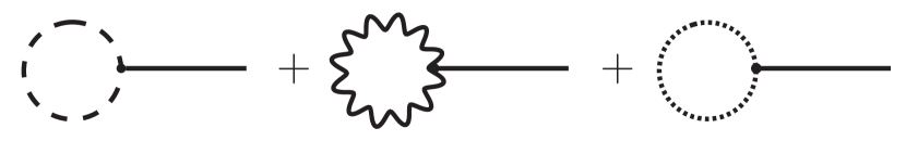
Figure 1: The diagrams contributing to the one point function of $\tilde{\chi}$. From left to right the diagrams involve a $\tilde{\phi}$ loop, an electroweak gauge particle loop and a top quark loop.

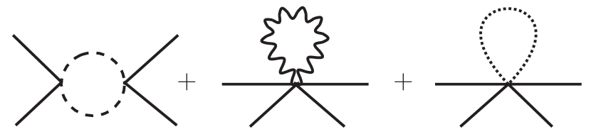
Figure 2: The diagrams contributing to $\tilde{\chi}\tilde{\chi}\rightarrow\tilde{\chi}\tilde{\chi}$ scattering. From left to right the diagrams involve a $\tilde{\phi}$ loop, an electroweak gauge boson loop and a top loop.

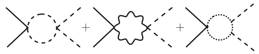
Figure 3: The diagrams contributing to $\tilde{\chi}\tilde{\chi}\rightarrow\tilde{\phi}\tilde{\phi}$ scattering. Here the left diagram involves a $\tilde{\phi}$ loop. The middle involves an electroweak gauge boson loop which go into a pair of Higgs bosons, which are represented here by the $\phi$ particles, through the standard electroweak vertex. The right diagram involves a top quark loop. The top quark emits two Higgs particles due to the Yukawa interaction.

We now check the order of magnitude of the one loop contributions. As explained earlier we are basically interested in determining the order of magnitude of the finite parts. If these are too large then we will require large counter terms which will lead to fine tuning. Let us first consider the one point function of the field $\tilde{\chi}$. The one loop corrections to this are shown in Fig. 1 The first term arises directly from the potential and is of order $\lambda_{1}\lambda_{2}v^{2}\eta$. This may be compared with the classical contribution to this amplitude which arises from the $\lambda\chi^{4}$ term. The relevant term is proportional to $\lambda\tilde{\chi}\eta^{3}$ and gives a contribution of order $v^{2}\eta\lambda_{2}$. It is clear that the loop correction is smaller than the leading order term. We also get contributions to the one point function due to the $\mathcal{L}_{EW}$ and $\mathcal{L}_{Y}$ Lagrangians displayed above. The one loop contributions arise due to the diagrams shown in Fig. 1. These contributions are found to be finite due to the presence of $\delta$ in the relevant Feynman rule in $d$ dimensions. The contributions of these terms are found to be of order $v^{4}/\eta\sim v^{2}\eta\lambda_{2}$ and hence are found to be the same order as the leading order term. Here we have set $M_{W}\sim m_{t}\sim v$, where $M_{W}$ and $m_{t}$ are the W-boson and top quark masses respectively. The higher order contributions of these terms will be suppressed by additional power of weak coupling or $g_{t}$. Hence we see that these do not lead to any fine tuning.

An important point is that there is no mass term in the Lagrangian due to conformal invariance. Hence the scalar field mass is not an independent parameter and we do not need to check the corrections to this parameter. In particular the Higgs mass is expected to be stable under quantum corrections due to conformal invariance [22, 86].

We next look at the four point function corresponding to $\tilde{\chi}$. The relevant one-loop corrections are shown in Fig. 2. The first term is of order $(\lambda_{1}\lambda_{2})^{2}$ which is small compared to $\lambda$. The other two terms are of order $v^{4}/\eta^{4}$ which is of the same order as $\lambda$. Hence none of these lead to any fine tuning problems. As in the case of the one point function, higher order contributions from all the terms would be further suppressed. This clearly shows that the parameter $\lambda$ does not require any fine tuning.

We next check the parameter $\lambda_{2}$. This contributes to the scattering process $\tilde{\chi}\tilde{\chi}\rightarrow\tilde{\phi}\tilde{\phi}$. The relevant one loop diagrams are shown in Fig. 3. The first diagram gets contribution directly from the potential and is of order $\lambda_{1}^{2}\lambda_{2}$ and hence suppressed compared to the leading order amplitude. The remaining diagrams arise due to the presence of the conformal regulator. As in the case of $\tilde{\chi}\tilde{\chi}\rightarrow\tilde{\chi}\tilde{\chi}$, these diagrams give finite contributions, which are smaller or comparable to the leading order amplitude. Furthermore at higher orders such contributions will be suppressed compared to the leading order result. Hence we see that the model does not require any fine tuning of parameters.

We next check the contributions due to the hidden strongly coupled sector. The $\chi$ field also couples to the hidden fermions by the Yukawa interaction terms. These terms can contribute to the $\tilde{\chi}\tilde{\chi}\rightarrow\tilde{\chi}\tilde{\chi}$ by the diagram shown in Fig. 4. This diagram gives a contribution of order $g_{Y}^{4}$. Hence we should require that $g_{Y}<\lambda^{1/4}\sim\lambda_{2}^{1/2}\sim v/\eta$. We find that in this limit, the minimum value of $\Lambda_{S}$ is given by, $\Lambda_{S}\sim v$. Such a small value of Yukawa couplings have interesting implications for the hidden sector meson spectrum. We point out that this sector has approximate chiral symmetry which is broken by the Yukawa couplings. In the limit of exact symmetry we expect zero mass pseudoscalar Goldstone bosons corresponding to broken global chiral symmetry. However due to explicit breaking these will acquire small masses. The interesting point is that the breaking a very tiny and hence the mass is expected to very very small in comparison to the scale $\Lambda_{S}\sim v$. This implies existence of dark matter particles whose masses are much smaller than the electroweak scale.

Figure 4: The box diagram contribution to the $\tilde{\chi}\tilde{\chi}\rightarrow\tilde{\chi}\tilde{\chi}$ scattering. The internal lines correspond to fermions in the dark strongly coupled sector.

We next consider the contributions from the hidden gauge sector. As we have shown above, for our typical choice of parameters $\lambda\sim\lambda_{2}^{2}$, $\lambda_{2}\sim v/\eta$, the minimum value of $\Lambda_{S}\sim v$. We expect that the mass scale of the gauge sector, $\Lambda^{\prime}_{S}$, to be also of this order. Hence all loop contributions would at most be of the same order as those obtained from the electroweak sector. As we have discussed in section 3, in order to evaluate these contributions we should split them into a non-perturbative and a perturbative part. Furthermore we have argued that the non-perturbative contributions are suppressed. Treating these gauge particles perturbatively we get contributions analogous to those obtained from the electroweak gauge bosons, as shown in Figs. 1, 2, 3. In order to test whether these lead to any fine tuning, we can set the external momentum equal to zero. Furthermore these gauge particles are massless within the framework of perturbation theory. Hence all the loop contributions analogous to those shown in Figs. 1, 2, 3 vanish within dimensional regularization. This is true also for all loops which involve only these particles. Loops which involve these particles along with other particles can lead to non-zero contributions. The dominant contributions are expected to arise from loops involving the hidden gauge particles and hidden fermions. The perturbative masses of these hidden fermions are of order $g_{Y}\eta<v$. Hence we expect these masses to be small compared to $v$. In this case these loops cannot give contributions larger in comparison to those obtained from the electroweak sector. As argued above these are sufficiently small and do not lead to any fine tuning problems.

We next consider the limit $\lambda\gg\lambda_{2}^{2}$. We assume that $\lambda$ is small compared to unity but sufficiently large so that there is no issue of acute fine tuning of this parameter. The box diagram shown in Fig. 4 leads to an amplitude of order $g_{Y}^{4}$. If $g_{Y}$ is of order unity and $\lambda$ very small compared to unity, this might require a mild fine tuning at one loop order. In order to avoid this we might demand that $g_{Y}<\lambda^{1/4}$. In this case we find that $\Lambda_{S}>g_{Y}\eta$. Assuming that $g_{Y}\gg\sqrt{\lambda_{2}}$, this implies that $\Lambda_{S}\gg v$. Hence in this case the mass scale of the hidden strong sector is much larger than the electroweak mass scale. Since $\lambda\gg\lambda_{2}^{2}$, the mixing of $\tilde{\chi}$ with $\tilde{\phi}$ is negligible. We find that the mass of $\tilde{\phi}$ (or Higgs) particle is given by $m_{\phi}^{2}\approx 2\lambda_{1}v^{2}$ and mass of $\tilde{\chi}$, $m_{\chi}^{2}\sim\lambda\eta^{2}$. Hence we find that in this case, $m_{\chi}\gg m_{\phi}$. A precise calculation of $m_{\chi}$ is complicated since $\tilde{\chi}$ also mixes with a scalar bound state of the strongly coupled hidden sector. Due to soft breaking of the conformal symmetry we expect one scalar particle of zero mass and another of order, $m^{2}\sim\lambda\eta^{2}$. The only very small parameter in this model is $\lambda_{2}\sim v^{2}/\eta^{2}$. This parameter essentially couples the field $\chi$ with the electroweak sector. At one loop the diagrams which can contribute to this parameter are shown in Fig. 3. It is easy to see that none of them lead to a large correction which may require fine tuning of $\lambda_{2}$.

Before ending this section we briefly consider the one loop corrections to the one point function of $\tilde{\chi}$ within the framework of the model with a super-Planckian value of $\eta$ discussed in section 2.1. The relevant diagrams are shown in Fig. 1. We find that the maximum value of these contributions is of order $v^{4}/\eta$, which are comparable to the leading order contributions. At higher order these will be further suppressed by powers of the electroweak coupling or the $\phi$ (or Higgs) self coupling or the top Yukawa coupling. Hence these contributions do not lead to any fine tuning of the parameter $\lambda$ in this model.

5   A constraint on the scale $\eta$

In this section we point out a constraint on the parameter space which arises due to the presence of the conformal regulator. This has so far not been realized in the literature. Let us consider the standard model Yukawa interaction term of the electron. This can be expressed as,

$$\mathcal{L}_{Y}=-\left[g_{e}(\bar{\nu}_{e}\ \bar{e})_{L}{\mathcal{H}}e_{R}+h.c.\right]\left(\zeta^{2}\right)^{-\delta/2}$$ (33)

Here $\mathcal{H}$ denotes the Higgs field and $\nu_{e}$ and $e$ the neutrino and electron fields respectively. Here we use the standard model Higgs field in contrast to the toy singlet Higgs, $\phi$, used in the rest of this paper. We need to suitable modify the form of $\zeta$ in Eq. 5 by replacing $\phi^{2}$ by ${\mathcal{H}}^{\dagger}\mathcal{H}$. We expand $\mathcal{H}$ about its vacuum expectation value $v$. This leads to the mass term for the electron. Now the important point is that in $d$ dimensions these mass terms couple to the field $\chi$. This coupling leads to a non-zero contribution to the scattering amplitude $ee\rightarrow ee$ displayed in Fig. 5. The wavy lines represent a photon or a weak gauge boson. We consider loops instead of the tree level process because the $ee\chi$ coupling is proportional to $(d-4)$ and hence goes to zero when $d\rightarrow 0$. However, with the two loops, the $(d-4)$ factors get cancelled by the $1/(d-4)$ factors arising due loop divergences. We are interested in scattering at low energy for which the dominant contribution arises from the exchange of photons.

The contribution from each loop in $d$ dimensions is proportional to,

$$\int d^{d}p\,{1\over p^{2}}\,{p^{2}\over(p^{2}-m_{e}^{2})^{2}}$$

where $m_{e}$ is the mass of the electron. In $d=4$ this integral is dimensionless. Here we have set the external momentum equal to zero. Each of the two $ee\chi$ vertices yield a factor of $m_{e}/\eta$. Besides that each photon exchange yields a factor of $\alpha$. Hence the order of magnitude of this amplitude is $(\alpha m_{e}/\eta)^{2}$. This is small but not entirely negligible since the coupling involves the mass of the electron and the effect accummulates in the case of macroscopic bodies.

Before discussing the implications of such amplitudes we consider the corresponding diagrams for the case of hadrons. In principle, such contributions may also arise for nucleons. A possible diagram is displayed in Fig. 6. The $NN\tilde{\chi}$ coupling arises due to the Yukawa interaction terms of the up and down quarks. Here we require an effective coupling of the nucleon with $\chi$ which will involve a form factor. The thick solid lines in Fig. 6 represent exchange of strongly interacting particles or a photon or a weak gauge bosons. For simplicity let us first consider a photon. We again set the external momentum equal to zero. At each of the photon vertices we need to include the nucleon electromagnetic form factor which decays as $1/p^{4}$ for large values of $p^{2}$. Inserting such a form factor into the loop integral, we find that the integral is finite and hence the total contribution from such diagrams vanish in the limit $d\rightarrow 4$. We expect the presence of similar form factors for the case of multi-gluon or meson exchanges also and hence such amplitudes vanish in the case of nucleons.

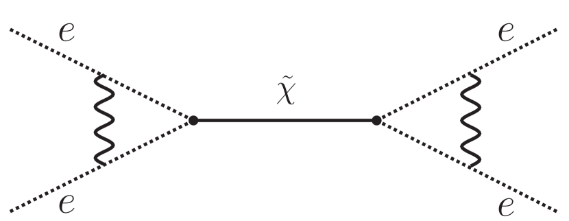
Figure 5: The electron-electron scattering by exchange of a scalar field $\tilde{\chi}$. The dotted lines represent an electron. The wavy lines represent a photon or a weak gauge boson. Here we show only a $s$-channel diagram. We can also have a $t$ and a $u$-channel process.

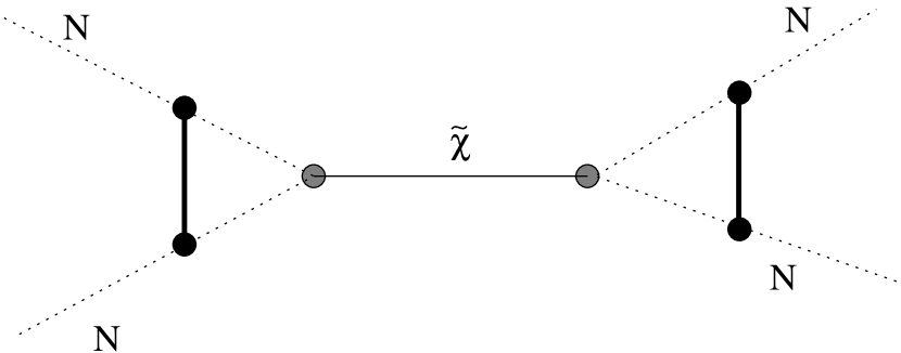
Figure 6: The nucleon-nucleon scattering by exchange of a scalar field $\tilde{\chi}$. The dotted lines represent a nucleon. The thick solid lines represent a multigluon exchange or a meson such as a pion or a $\rho$ meson etc. These may also represent exchange of a photon or a weak gauge boson. The blobs represent effective vertices which involve the nucleon form factors.

For macroscopic bodies we expect a small deviation from the standard law of gravity arising due to the coupling of $\chi$ to the mass of electrons. This additional contribution is very tiny if we choose $\eta\sim M_{PL}$. In this case the amplitude and hence the corresponding potential will be suppressed by more than 10 orders of magnitude in comparison to the standard gravitational potential. This is due to factors of $\alpha^{2}$ and an additional suppression factors of $m_{e}/m_{N}$ in comparison to standard gravitational interaction. Here $m_{N}$ is the mass of the nucleon. Furthermore the particle $\tilde{\chi}$ is massive with mass equal to $3\lambda\eta^{2}$. With $\lambda\sim v^{4}/\eta^{4}$ and $\eta\sim M_{PL}$, this leads to a mass of about $10^{-6}$ eV. Hence the interaction is appreciable only over a distance of a few cm. It is clear that this choice of parameters are allowed. However if $\eta$ is taken to be much smaller than it might conflict with experimental constraints. We postpone a detailed discussion of such contraints to future work.

We point out that there exists a massless scalar particle in our theory due to soft breaking of scale invariance. This particle is expected to be a mixture of $\tilde{\chi}$, $\tilde{\phi}$ and a bound state of the dark sector fermions. It can also contribute to the amplitudes shown in Figs. 5 and 6 due to its mixing with $\tilde{\chi}$. In this case the interaction would have an infinite range since the particle being exchanged is massless. However we expect that the mixing is small and hence the amplitude would be further suppressed in comparison to the amplitude due to the exchange of $\tilde{\chi}$. We also point out that such amplitudes would be negligible if we impose local conformal invariance since in this case the massless particle would not be present in the physical spectrum and act as the longitudinal mode of the Weyl meson. Furthermore all our arguments with regards to the absence of fine tuning of parameters $\lambda$ and $\lambda_{2}$ apply even in the case of local conformal invariance.

6   Including the Standard Model fields

In our discussion so far we have considered a toy model in which the Higgs multiplet is represented by a real scalar field. However the main results of our paper are applicable in the full standard model also. We briefly illustrate this in this section. The conformal extension of the standard model in $d$ dimensions can be expressed as, [26].

$${\cal S}={\mathcal{S}}_{G}+{\mathcal{S}}_{C}$$ (34)

where ${\mathcal{S}}_{G}$ is the gravitational action and ${\mathcal{S}}_{C}$ represents the conformal extension of the standard model. It is given by,

$$\mathcal{S}_{SM} = \int d^{d}x\sqrt{-g}\Bigg{[}{1\over 2}g^{\mu\nu}\partial_{\mu}\chi\partial_{\nu}\chi+g^{\mu\nu}(D_{\mu}\mathcal{H})^{\dagger}(D_{\nu}\mathcal{H})-\frac{1}{4}g^{\mu\nu}g^{\alpha\beta}(\mathcal{A}^{i}_{\mu\alpha}\mathcal{A}^{i}_{\nu\beta}$$ (35)

$$+ \mathcal{B}_{\mu\alpha}\mathcal{B}_{\nu\beta}+\mathcal{G}^{j}_{\mu\alpha}\mathcal{G}^{j}_{\nu\beta})(\zeta^{2})^{\delta}-{\lambda_{1}\over 4}(4\mathcal{H}^{\dagger}\mathcal{H}-\lambda_{2}\chi^{2})^{2}(\zeta^{2})^{-\delta}-{\lambda\over 4}\chi^{4}(\zeta^{2})^{-\delta}\Bigg{]}$$

$$+ {\cal S}_{\rm fermions},$$

where $\mathcal{H}$ is the Higgs multiplet and $\mathcal{G}^{j}_{\mu\nu}$, $\mathcal{A}^{i}_{\mu\nu}$ and $\mathcal{B}_{\mu\nu}$ and $\mathcal{E}_{\mu\nu}$ are the standard field strength tensors for the $SU(3)$, $SU(2)$ and $U(1)$ gauge fields. Here $\zeta$ is same as given in Eq. 5 with $\phi^{2}$ replaced by ${\mathcal{H}}^{\dagger}\mathcal{H}$. We point out that these gauge fields remain unchanged under conformal transformation. The fermion action, ${\cal S}_{\rm fermions}$, is given by

$${\cal S}_{\rm fermions} = \int d^{d}x\,e\,\left({\overline{\Psi}}_{\rm L}i\gamma^{\mu}{\cal D_{\mu}}\Psi_{\rm L}+{\overline{\Psi}}_{\rm R}i\gamma^{\mu}{\cal D_{\mu}}\Psi_{\rm R}\right)$$ (36)

$$-\int d^{d}x\,e\,(g_{Y}\overline{\Psi}_{\rm L}{\mathcal{H}}\Psi_{\rm R}(\zeta^{2})^{-\delta/2}+h.c.),$$

where $e={\rm det}(e_{\mu}^{~{}a})$, $e_{\mu}^{~{}a}e_{\nu}^{~{}b}\eta_{ab}=g_{\mu\nu}$, $\gamma^{\mu}=e^{\mu}_{~{}a}\gamma^{a}$, $e_{\mu}^{a}$ is the vielbein and $a,b$ are Lorentz indices. Here $\Psi_{L}$ and $\Psi_{R}$ represent the left and right handed projections of the fermion field and $g_{Y}$ is a Yukawa coupling. The gauge covariant derivatives of fermion fields are same as in the standard model. Here also we have assumed global conformal invariance but the model can be easily generalized to display local invariance. In Eq. 36 we have shown only a representative term of the fermion field. Additional terms corresponding to different Yukawa couplings and different families can be added analogously.

It is clear from the action that the analysis presented in sections 2 and 3 is applicable in this case also. Here we have essentially replaced the real scalar $\phi$ with the Higgs field. The Higgs field acquire VEV once the classical value of $\chi$ is non-zero. As discussed in section 2, we can evade the fine tuning problem if we choose the classical value of $\chi$ to be much larger than the Planck mass. Alternatively, as discussed in section 3 we add a dark strongly coupled sector, which triggers the breakdown of electroweak symmetry through the vacuum expectation value of $\chi$.

7   Conclusions

In this paper we have explained how the fine tuning problem of the cosmological constant manifests itself in a conformal model. We have assumed a matter action which displays global conformal invariance in $d$ dimensions. In such a model the trace of the energy momentum tensor is zero even for the dimensionally regulated action. Hence the model leads to vanishing cosmological constant even at loop orders. However the problem of fine tuning of cosmological constant manifests itself in the requirement to break the conformal symmetry by a soft mechanism. In the simplest version of the model, this is implemented by generating a non-zero classical value of the real scalar field $\chi$, which in turn leads to a breakdown of the electroweak symmetry. This mechanism requires two very small parameters. One of these parameters, denoted by $\lambda_{2}$ in our paper, is equal to $(v/\eta)^{2}$, where $\eta$ is some very large mass scale, which may be taken to be $M_{PL}$. Although this parameter is small, we find that it does not get large corrections at loop orders and hence does not require fine tuning. However there exists another parameter, denoted as $\lambda$ in our paper, which leads to acute fine tuning problems. If this parameter is not fine tuned, the field $\chi$ quickly decays to zero and the conformal symmetry is restored. We argue that this situation is avoided if the classical value of $\chi$ is much larger than $M_{PL}$.

We also discuss another model in which there exists a dark strongly coupled sector. In this case the conformal symmetry breaking is triggered by the formation of condensates in this sector. In this case also the full model, including the hidden as well as the standard model sector displays exact conformal invariance in $d$ dimensions. The generation of condensates lead to a non-zero vacuum value of $\chi$ which leads to a breakdown of electroweak symmetry. With this mechanism also we find that none of the parameter suffer from fine tuning problems at loop orders. We describe the parameter ranges over which this is applicable. We have discussed a specific model which involves a strongly coupled sector. However our mechanism may be applicable to other models also which involve interactions similar to technicolor provided the conformal invariance is maintained within the regulated action. Furthermore it may also be interesting to consider the model with local conformal invariance. The mechanism discussed in our paper should be applicable in this case also.

In our analysis we have focussed primarily on the problem associated with the fine tuning of the cosmological constant. We have shown that it is possible to set it to zero without having to arbitrarily set some parameter to zero order by order in perturbation theory. We have so far not addressed the issue of how the dark energy and dark matter may be generated in our model. Our main point is that the class of models which we present provide us with a useful starting point in which to address these issues. There does exist a dark sector which might be responsible for these components. However the problem is a little complicated since the trace of the energy momentum tensor and hence $R$ is very close to zero in these models. The deviation from zero is controlled by the gravitational action which is not conformally invariant or is obtained by making a particular gauge choice within the framework of local conformal invariance [12]. It is clear that such terms will generate a value of $R$ of the order that is acceptable by cosmological considerations. However more work is required in order to fit the cosmological data within this framework.

8   Appendix: Feynman Rules

In this Appendix we summarize the Feynman rules in our theory. These correspond to the Lagrangian densities, $\mathcal{L}_{EW}$, $\mathcal{L}_{V}$ and $\mathcal{L}_{Y}$ displayed in Eq. 31, 30 and 32 respectively. The field $\zeta$ is defined in Eq. 5 and we need to expand terms such as, $(\zeta^{2})^{\delta}$. The leading order terms in such an expansion are displayed in Eq. 11. Here the dominant contributions arise from the $\hat{\chi}$ terms and hence we ignore the $\hat{\phi}$ terms. We next express $\hat{\chi}$ in terms of $\tilde{\chi}$ using Eq. 27. At leading order the two are equal to one another.

We denote the $\tilde{\chi}$ and $\tilde{\phi}$ lines by a solid and dashed lines respectively. An electroweak gauge boson is denoted by a wavy line and a fermion by a dotted line as shown in Fig. 7. The Feynman rules for the couplings of $\tilde{\chi}$ which arise from the Lagrangian given in Eq. 31 are shown in Figs. 8, 9, 10. The corresponding rule due to the Yukawa term, Eq. 32, is given in Fig. 11. Finally the Feynman rules arising from the scalar field potential terms are given in Fig. 12.

Figure 7: The conventions used in the Feynman diagrams. Here $A_{\mu}^{a}$ represents an electroweak gauge boson.

$$=-i\delta(-1)^{n}\frac{2(n-1)!}{\eta^{(n-2\delta)}}\times\Big{(}2\left(k\cdot p\right)g^{\mu\nu}-k^{\mu}p^{\nu}-k^{\nu}p^{\mu}\Big{)}$$

Figure 8: The scattering of two electroweak gauge bosons with $n$ $\tilde{\chi}$ particles. This vertex arises due to electroweak gauge boson kinetic energy term in $d$ dimensions.

$$\begin{split}=\delta(-1)^{n}&\frac{2(n-1)!}{\eta^{(n-2\delta)}}\,gf^{abc}\\ &\times\Big{(}g^{\mu\nu}(k-p)^{\rho}+g^{\nu\rho}(p-q)^{\mu}+g^{\rho\mu}(q-k)^{\nu}\Big{)}\end{split}$$

Figure 9: The scattering of three electroweak gauge bosons with $n$ $\tilde{\chi}$ particles.

$$\begin{split}=-i\delta(-1)^{n}\frac{2(n-1)!}{\eta^{(n-2\delta)}}\times&g^{2}\Big{(}f^{abe}f^{cde}\left(g^{\nu\rho}g^{\nu\sigma}-g^{\mu\sigma}g^{\nu\rho}\right)\\ &+f^{ace}f^{bde}\left(g^{\mu\nu}g^{\rho\sigma}-g^{\mu\sigma}g^{\nu\rho}\right)\\ &+f^{ade}f^{bce}\left(g^{\mu\nu}g^{\rho\sigma}-g^{\mu\rho}g^{\nu\sigma}\right)\Big{)}\end{split}$$

Figure 10: The scattering of four electroweak gauge bosons with $n$ $\tilde{\chi}$ particles.

$$=-i\delta(-1)^{n}(n-1)!\frac{g_{t}v}{\eta^{n+\delta}}$$

Figure 11: The scattering of a top and an anti-top quark with $n$ $\tilde{\chi}$ particles.

Figure 12: The Feynman rules arising from the scalar field potential terms.

Acknowledgements: Gopal Kashyap thanks the Council of Scientific and Industrial Research (CSIR), India for providing his Ph.D. fellowship. PJ thanks Shrihari Gopalakrishna, S. Kalyana Rama and Romesh Kaul for a stimulating discussion.

References

- [1] H. Weyl, Z. Phys. 56, 330 (1929) [Surveys High Energ. Phys. 5, 261 (1986)].
- [2] S. Deser, Annals Phys. 59, 248 (1970).
- [3] P. A. M. Dirac, Proc. Roy. Soc. Lond. A 333, 403 (1973).
- [4] D. K. Sen and K. A. Dunn, J. Math. Phys. 12, 578 (1971).
- [5] R. Utiyama, Prog. Theor. Phys. 50, 2080 (1973).
- [6] R. Utiyama, Prog. Theor. Phys. 53, 565 (1975).
- [7] P. G. O. Freund, Annals Phys. 84, 440 (1974).
- [8] F. Englert, C. Truffin and R. Gastmans, Nucl. Phys. B 117, 407 (1976).
- [9] K. Hayashi, M. Kasuya and T. Shirafuji, Prog. Theor. Phys. 57, 431 (1977) [Erratum-ibid. 59, 681 (1978)].
- [10] K. Hayashi and T. Kugo, Prog. Theor. Phys. 61, 334 (1979).
- [11] M. Nishioka, Fortsch. Phys. 33, 241 (1985).
- [12] T. Padmanabhan, Class. Quant. Grav. 2, L105 (1985).
- [13] D. Ranganathan, J. Math. Phys. 28, 2437 (1987).
- [14] H. Cheng, Phys. Rev. Lett 61, 2182 (1988).
- [15] G. t’ Hooft, arXiv:1410.6675 (2014).
- [16] S. Weinberg, Rev. Mod. Phys. 61, 1 (1989).
- [17] T. Padmanabhan, Phys. Rept. 380, 235 (2003) [arXiv:hep-th/0212290].
- [18] C. Wetterich, Nucl. Phys. B 302, 668 (1988).
- [19] P. D. Mannheim, Gen. Rel. Grav. 22, 289 (1990).
- [20] P. Jain and S. Mitra, Mod. Phys. Lett. A 22, 1651 (2007) [arXiv:0704.2273 [hep-ph]].
- [21] P. Jain, S. Mitra and N. K. Singh, JCAP 0803, 011 (2008) [arXiv:0801.2041 [astro-ph]].
- [22] M. E. Shaposhnikov and D. Zenhausern, Phys. Lett. B 671, 162 (2009) [arXiv:0809.3406 [hep-th]].
- [23] M. E. Shaposhnikov and D. Zenhausern, Phys. Lett. B 671, 187 (2009) [arXiv:0809.3395 [hep-th]].
- [24] P. Jain and S. Mitra, Mod. Phys. Lett. A 24, 2069 (2009) [arXiv:0902.2525 [hep-ph]].
- [25] H. Nishino and S. Rajpoot, Phys. Rev. D 79, 125025 (2009).
- [26] P. K. Aluri, P. Jain, S. Mitra, S. Panda and N. K. Singh, Mod. Phys. Lett. A 25, 1349 (2010) [arXiv:0909.1070 [hep-ph]].
- [27] P. Jain, S. Mitra, S. Panda and N. K. Singh, arXiv:1010.3483 [hep-ph].
- [28] P. D. Mannheim, Gen. Rel. Grav. 43, 703 (2011) [arXiv:0909.0212 [hep-th]].
- [29] H. Nishino and S. Rajpoot, Class. Quan. Grav. 28, 145014 (2011).
- [30] I. Bars, P. Steinhardt, and N. Turok, Phys. Rev. D 89, 043515 (2014).
- [31] P. Jain and G. Kashyap, Mod. Phys. Lett. A. 29 1450195 (2014).
- [32] B. Ratra and P. J. E. Peebles, Phys. Rev. D 37, 3406 (1988).
- [33] P. J. E. Peebles and B. Ratra, Rev. Mod. Phys. 75, 559 (2003).
- [34] E. J. Copeland, M. Sami and S. Tsujikawa, Int. J. Mod. Phys. D 15, 1753 (2006).
- [35] M. E. Shaposhnikov and F. V. Tkachov, arXiv:0905.4857.
- [36] P. Jain and S. Mitra Mod. Phys. Lett. A 25, 167 (2010) [arXiv:0903.1683 [hep-ph]].
- [37] N. K. Singh, P. Jain, S. Mitra and S. Panda, Phys. Rev. D 84, 105037 (2011).
- [38] C. G. Callan, S. Coleman and R. Jackiw, Annals of Physics 59, 42 (1970).
- [39] C. Tamarit, JHEP 12, 098 (2013).
- [40] E. Farhi and L. Susskind, Physics Reports, 74, 277 (1981).
- [41] K. A. Meissner and H. Nicolai, Phys. Lett. B648. 312 (2007).
- [42] K. A. Meissner and H. Nicolai, Phys. Lett. B660. 260 (2008).
- [43] T. Hur and P. Ko, Phys. Rev. Lett. 106, 141802 (2011).
- [44] C. g. Huang, D. d. Wu and H. q. Zheng, Commun. Theor. Phys. 14, 373 (1990).
- [45] D. Hochberg and G. Plunien, Phys. Rev. D 43, 3358 (1991).
- [46] W. R. Wood and G. Papini, Phys. Rev. D 45, 3617 (1992).
- [47] J. T. Wheeler, J. Math. Phys. 39, 299 (1998) [arXiv:hep-th/9706214].
- [48] A. Feoli, W. R. Wood and G. Papini, J. Math. Phys. 39, 3322 (1998) [arXiv:gr-qc/9805035].
- [49] M. Pawlowski, Turk. J. Phys. 23, 895 (1999) [arXiv:hep-ph/9804256].
- [50] D. A. Demir, Phys. Lett. B 584, 133 (2004) [arXiv:hep-ph/0401163].
- [51] H. Wei and R. G. Cai, JCAP 0709, 015 (2007) [arXiv:astro-ph/0607064].
- [52] T. Y. Moon, J. Lee and P. Oh, Modern Physics Letters A 25, 3129 (2010).
- [53] T. Maki, N. Kan and K. Shiraishi, J. Mod. Phys. 3, 1081 (2012).
- [54] G. Kashyap, Phys. Rev. D 87, 016018 (2013).
- [55] I. Quiros, 2014, arXiv:1401.2643[gr-qc].
- [56] S. Dengiz, arXiv:1404.2714.
- [57] G. Kashyap, arXiv:1405.0679.
- [58] A. Salvio and A. Strumia, JHEP 1406, 080 (2014).
- [59] A. Codello, G. D’Odorico, C. Pagani and R. Percacci, Class. Quant. Grav. 30, 115015 (2013).
- [60] A. Padilla, D. Stefanyszyn and M. Tsoukalas, Phys.Rev. D 89 065009 (2014).
- [61] J. Garcia-Bellido, J. Rubio, M. Shaposhnikov and D. Zenhausern, Phys. Rev. D 84 123504 (2011), arXiv:1107.2163 .
- [62] J. Garcia-Bellido, J. Rubio and M. Shaposhnikov, Phys. Lett. B 718 507 (2012), arXiv:1209.2119.
- [63] P. Jain, A. Jaiswal, P. Karmakar, G. Kashyap, and N. K. Singh, JCAP, 1211, 003 (2012).
- [64] R. Armillis, A. Monin and M. Shaposhnikov, JHEP 1310, 030 (2013).
- [65] T. Henz, J. M. Pawlowski. A. Rodigast and C. Wetterich, Phys. Lett. B 727 298 (2013).
- [66] D. Gorbunov and A. Tokareva, arXiv:1307.5298.
- [67] F. Gretsch and A. Monin, arXiv:1308.3863.
- [68] V. V. Khoze, JHEP 1311, 215 (2013).
- [69] A. Aurilia, H. Nicolai and P. K. Townsend, Nucl. Phys. B 176, 509 (1980).
- [70] J. J. van der Bij, H. van Dam and Y. J. Ng, Physica 116A, 307 (1982).
- [71] M. Henneaux and C. Teitelboim, Phys. Lett. B 143, 415 (1984).
- [72] J. D. Brown and C. Teitelboim, Nucl. Phys. B 297, 787 (1988).
- [73] W. Buchmuller and N. Dragon, Phys. Lett. B 207, 292 (1988).
- [74] W. Buchmuller and N. Dragon, Phys. Lett. B 223, 313 (1989).
- [75] M. Henneaux and C. Teitelboim, Phys. Lett. B 222, 195 (1989).
- [76] A. Daughton, J. Louko and R. D. Sorkin, Talk given at 5th Canadian Conference on General Relativity and Relativistic Astrophysics (5CCGRRA), Waterloo, Canada, 13-15 May 1993, Canadian Gen. Rel. 0181, (1993) [arXiv:gr-qc/9305016].
- [77] V. Sahni and S. Habib, Phys. Rev. Lett. 81, 1766 (1998) [arXiv:hep-ph/9808204].
- [78] D. E. Kaplan and R. Sundrum, JHEP 0607, 042 (2006) [arXiv:hep-th/0505265].
- [79] F. K. Diakonos and E. N. Saridakis, JCAP 0902, 030 (2009).
- [80] J. D. Barrow and D. J. Shaw, Phys. Rev. Lett. 106, 101302 (2011).
- [81] D. J. Shaw and J. D. Barrow, Phys. Rev. D 83, 043518 (2011).
- [82] D. A. Demir, Phys. Lett. B 701, 496 (2011).
- [83] I. K. Wehus and F. Ravndal, J. Phys. Conf. Ser. 66, 012024 (2007), arXiv:0610048.
- [84] D. A. Akyeampong and R. Delbourgo, Nuovo Cim. A 19, 219 (1974).
- [85] K. Nishijima, Fields and Particles, W. A. Benjamin, Inc., (1969).
- [86] G. M. Tavares, M. Schmaltz and W. Skiba, Phys. Rev. D 89, 015009 (2014).