Two charges on plane in a magnetic field: III. $He^{+}$ ion

Abstract

The $He^{+}$ ion on a plane subject to a constant magnetic field $B$ perpendicular to the plane is considered taking into account the finite nuclear mass. Factorization of eigenfunctions permits to reduce the four-dimensional problem to three-dimensional one. The ground state energy of the composite system is calculated in a wide range of magnetic fields from $B=0.01$ up to $B=100$ a.u. and center-of-mass Pseudomomentum $K$ from $0$ to $1000$ a.u. using a variational approach. The accuracy of calculations for $B=0.1$ a.u. is cross-checked in Lagrange-mesh method and not less than five significant figures are reproduced in energy. Similarly to the case of moving neutral system on the plane a phenomenon of a sharp change of energy behavior as a function of $K$ for a certain critical $K_{c}$ but a fixed magnetic field occurs.

Introduction

We study a two body Coulomb system on the plane subject to a constant magnetic field perpendicular to the plane. Main focus of this paper is on the charged system, in particular the $He^{+}$ ion.

In classical mechanics a planar system of two Coulomb charges $(e_{1},m_{1})$ and $(e_{2},m_{2})$ in the presence of a constant magnetic field $B$ perpendicular to the plane is bounded for any value of magnetic field $B>0$ (see e.g. PM:2006 ). In the case of particles with opposite charges ($e_{1}\,e_{2}<0$) for certain initial conditions special concentric (closed) trajectories occur (see ET:2013 and references therein), they are shown in Fig. 1. It manifests the appearance of extra conserved quantities specific for these trajectories (particular integrals of motion)

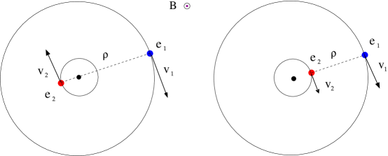
Figure 1: For a $He^{+}$-like ion ($e_{1}=-2\,e_{2}$) a family of periodic circular trajectories occurs in which the particles rotate with the same angular frequency on concentric circles with (left) relative phase $\pi$ or (right) zero relative phase. The relative distance between particles remains unchanged during the evolution.

In quantum mechanics, the appearance of particular integrals signals the existence of quasi-exactly-solvable solutions. In the cases of neutral atom ($e_{1}+e_{2}=0$) at rest and of quasi-equal charges $(\frac{e_{1}}{m_{1}}=\frac{e_{2}}{m_{2}})$ common analytical solutions of Hamiltonian and particular integrals emerge for certain discrete values of magnetic field strength ET-q:2013 -Turbiner:1994 . They also present the periodic circular trajectory Fig. 1 (left). Therefore, the trajectories (Fig.1) may indicate that the physically important case of the $He^{+}$ ion ($\alpha,e$) in magnetic field possesses analytical eigenfunctions. However, a single exact solution has not been found yet.

It is worth describing the 3D case. In the three-dimensional case, quantum mechanical charged systems in magnetic field have been reviewed by Garstang Garstang in the infinite nucleus mass approximation. In the case of finite nuclear mass the CM motion cannot be separated from the relative motion. The investigation of the effects of CM motion on the properties of two-body systems in magnetic field started with a detailed mathematical study Avron . To the best of our knowledge there was a single attempt Bezchastnov to study the $He^{+}$ ion taking into account the finite mass effects. It was based on multiconfigurational Hartree-Fock method and carried out for the case of strong fields, $B\gtrsim 500$ a.u.

In spite of the fact that there exists a number of properties which are common for two- and three-dimensional systems in a constant uniform magnetic field a connection between two- and three-dimensional cases is unknown. The aim of the present work is not to study those common properties, but they will be mentioned below.

For the planar quantum $He^{+}$ ion in a magnetic field perpendicular to the plane calculations of eigenfunctions are not available. Unlike the cases of neutral atom ($e_{1}+e_{2}=0$) at rest and of quasi-equal charges $(\frac{e_{1}}{m_{1}}=\frac{e_{2}}{m_{2}})$ the CM motion of the $He^{+}$ ion cannot be (pseudo)separated from the relative motion as well. The situation gets complicated due to the absence of (particular) integrability Turbiner:PI . Nevertheless, one component of the conserved Pseudomomentum $\mathbf{K}$ found by Gor’kov & Dzyaloshinskii GD:1967 for 3D neutral system remains integral for a planar charged systems. It allows us to reduce this four-dimensional problem to a three-dimensional one.

In a previous paper ET-gen:2013 an accurate variational solution, complementary to the exact solutions, for several low-lying states for both quasi-equal charges $(\frac{e_{1}}{m_{1}}=\frac{e_{2}}{m_{2}})$ and neutral system at rest was given. The accuracy of obtained results was evaluated in a specially designed, convergent perturbation theory. In ET-genq:2013 the moving neutral system was considered. By studying the ground state energy it was shown the stability of the system for all studied magnetic fields.

The goal of the present paper, which is the natural continuation of ET-gen:2013 -ET-genq:2013 , is to perform a detailed study of the ground state of the $He^{+}$ ion for different magnetic fields and Pseudomomentum, checking its stability. It has to be emphasized that the variational functions are chosen to be also eigenfunctions of one component of Pseudomomentum. It is worth mentioning that the $He^{+}$ ion in 3D is seen as an important system for astrophysics Neutron for large values of the magnetic field.

We are going to employ a variational method with an optimization of the form of the vector potential (optimal gauge fixing) constructing the trial function in such a way to combine a WKB expansion at large distances with perturbation theory expansion at small distances near the minima of the potential into an interpolation Turbiner:1988-2010 .

I Generalities

The Hamiltonian, which describes the planar $He^{+}$ ion, $(e_{1}=-e\,,m_{1})$ and $(e_{2}=2e,\,m_{2})$ , in a constant and uniform magnetic field ${\bf B}=B\,\hat{\bf z}$ perpendicular to the plane, has the form

$${{\hat{H}}}= \frac{{({\mathbf{\hat{p}}_{1}}+\frac{e}{c}\,{\mathbf{A}(\boldsymbol{\rho}_{1})})}^{2}}{2\,m_{1}}+\frac{{({\mathbf{\hat{p}}_{2}}-\frac{2\,e}{c}\,{\mathbf{A}(\boldsymbol{\rho}_{2})})}^{2}}{2\,m_{2}}-\frac{2\,e^{2}}{\mid{\boldsymbol{\rho}}_{1}-{\boldsymbol{\rho}}_{2}\mid}+{\hat{H}}_{spin}\,,\qquad\boldsymbol{\rho}_{1,2}\in\Re^{2}\ ,$$ (1)

($e>0$) where $\hslash=\frac{1}{4\,\pi\,\epsilon_{0}}=1$, ${\mathbf{\hat{p}}}_{1,2}=-i\,\nabla_{1,2}$ is the canonical momentum, ${\boldsymbol{\rho}}_{1,2}$ the position vector, $m_{1,2}$ the mass of the first (second) particle, respectively. $\mathbf{A}\in\Re^{2}$ is the vector potential which corresponds to a constant magnetic field ${\bf B}$. The spin contribution ${\hat{H}}_{spin}=g\,(\mathbf{s}_{1}+\mathbf{s}_{2})\cdot\mathbf{B}$ is disregarded in the following because its contribution is trivial.

It is easy to check that the total Pseudomomentum,

$${\mathbf{\hat{K}}}\ \equiv\ \mathbf{k}_{1}+\mathbf{k}_{2}\ =\ \bigg{[}\mathbf{\hat{p}}_{1}+\frac{e}{c}\,\mathbf{A}(\boldsymbol{\rho}_{1})-e\,{\mathbf{B}}\times{{\boldsymbol{\rho}}_{1}}\bigg{]}+\bigg{[}(\mathbf{\hat{p}}_{2}-\frac{2\,e}{c}\,\mathbf{A}(\boldsymbol{\rho}_{2})+2\,e\,{\mathbf{B}}\times{{\boldsymbol{\rho}}_{2}}\bigg{]}\ ,$$ (2)

is a gauge-independent integral of motion belonging to the plane, on where the dynamics is developed,

$$[{\mathbf{\hat{K}}}\ ,\ {\hat{H}}]\ =\ 0\ .$$

For a single charged particle $q$ in a constant magnetic field the guiding center $\boldsymbol{\rho}_{{}_{c}}$, the center of the classical trajectory, can be written in terms of the pseudomomentum $\boldsymbol{\rho}_{{}_{c}}=\frac{{\mathbf{k}_{q}}\times\mathbf{B}}{e\,B^{2}}$. For the two-body neutral system, ${\mathbf{\hat{K}}}$ coincides (up to a unitary transformation) with the total canonical momentum and for $B=0$ becomes the total kinematic momentum ET:2013 . In general, the components of Pseudomomentum, closely connected to the phase space symmetries of the underlying classical and quantum Hamiltonians, are the generators of the phase space translation group Avron .

The following quantity is also an integral

$$\boldsymbol{\hat{\Omega}}\ =\ \bigg{[}{{\boldsymbol{\rho}}_{1}}\times({\mathbf{\hat{p}}_{1}}+\frac{e}{c}\,{\mathbf{A}(\boldsymbol{\rho}_{1})})-\frac{e\,B}{2\,c}\rho_{1}^{2}\,\hat{\bf z}\bigg{]}+\bigg{[}{{\boldsymbol{\rho}}_{2}}\times({\mathbf{\hat{p}}_{2}}-\frac{2\,e}{c}\,{\mathbf{A}(\boldsymbol{\rho}_{2})})+\frac{e\,B}{c}\rho_{2}^{2}\,\hat{\bf z}\bigg{]}\ ,$$ (3)

$[\,\boldsymbol{\hat{\Omega}},\,{\hat{H}}\,]=0$. The vector $\boldsymbol{\hat{\Omega}}$ is perpendicular to the plane. In the symmetric gauge ($\xi=\frac{1}{2}$), $\boldsymbol{\hat{\Omega}}$ becomes the total canonical angular momentum of the system.

It is easy to check that the operators $\mathbf{\hat{K}}=(\hat{K}_{x},\,\hat{K}_{y}),\ \boldsymbol{\hat{\Omega}}=\hat{\Omega}\,\hat{\bf z}$ obey the commutation relations

$$[{\hat{K}}_{x},\,{\hat{K}}_{y}]=-e\,B\,,$$ (4)

$$[{\hat{\Omega}},\,{\hat{K}}_{x}]={\hat{K}}_{y}\,,$$

$$[{\hat{\Omega}},\,{\hat{K}}_{y}]=-{\hat{K}}_{x}\ ,$$

Hence, they span a noncommutative algebra. The problem is not completely integrable. The Casimir operator ${\cal{\hat{C}}}$ of this algebra is nothing but

$${\cal{\hat{C}}}\ =\ {\hat{K}}_{x}^{2}+{\hat{K}}_{y}^{2}-\frac{2\,e\,B}{c}{\hat{\Omega}}\ .$$ (5)

It is clear that the integrals (4) form a subset of those already present in the three-dimensional case Avron .

Now, let us introduce on the plane cartesian coordinates and consider a certain one-parameter family of vector potentials corresponding to a constant magnetic field ${\bf B}=B\,\hat{\bf z}$ PRepts

$$\mathbf{A}_{\mathbf{r}}\equiv\mathbf{A}(\mathbf{r})\,=\,B\,((\xi-1)\,y\,,\,\xi\,x,\,0)\ ,$$

where $0\eqslantless\xi\eqslantless 1$ is a real parameter and $\mathbf{r}=(x,y)$. If $\xi=\frac{1}{2}$ we get the well-known and widely used gauge which is called symmetric or circular. If $\xi=0\ \text{or}\ 1$, we get the asymmetric or Landau gauge.

It is convenient to introduce center-of-mass (c.m.s.) coordinates

$$\mathbf{R}=\mu_{1}\,{\boldsymbol{\rho}}_{1}+\mu_{2}\,{\boldsymbol{\rho}}_{2}\ ,\quad{\boldsymbol{\rho}}={\boldsymbol{\rho}}_{1}-{\boldsymbol{\rho}}_{2}\ ,$$ (6)

$$\mathbf{\hat{P}}={\mathbf{\hat{p}}}_{1}+{\mathbf{\hat{p}}}_{2}\ ,\qquad\quad\,\,{\mathbf{\hat{p}}}=\mu_{2}\,{\mathbf{\hat{p}}}_{1}-\mu_{1}\,{\mathbf{\hat{p}}}_{2}\ ,$$

where $\mu_{i}=\frac{m_{i}}{M}$ is the ratio of the mass of the $i$th charge to the total mass of the system $M=m_{1}+m_{2}$. In these coordinates

$$\mathbf{\hat{K}}=\mathbf{\hat{P}}\ -\frac{e}{c}\,\mathbf{A}_{\bf R}+\frac{e}{c}\,\mathbf{B}\times\mathbf{R}+\frac{e\,\mu}{c}\,\mathbf{A}_{\boldsymbol{\rho}}-\frac{e\,\mu}{c}\,\mathbf{B}\times{\boldsymbol{\rho}}\ ,$$ (7)

$$\boldsymbol{\hat{\Omega}}\ = \bigg{[}\mathbf{R}\times({\mathbf{\hat{P}}}-\frac{e}{c}\,{\mathbf{A}_{\mathbf{R}}})+\frac{e\,B}{2\,c}R^{2}\,\hat{\bf z}\bigg{]}+\bigg{[}{\boldsymbol{\rho}}\times({\mathbf{\hat{p}}}-\frac{q_{\text{w}}}{c}\,{\mathbf{A}_{\boldsymbol{\rho}}})+\frac{q_{\text{w}}\,B}{2\,c}\rho^{2}\,\hat{\bf z}\bigg{]}$$ (8)

$$+\frac{2\,e\,\mu}{c}\,\mathbf{R}\times{\mathbf{A}_{\boldsymbol{\rho}}}-\frac{e\,\mu\,B}{c}(\mathbf{R}\cdot{\boldsymbol{\rho}})\,\hat{\bf z}\ ,$$

(cf. (2), (3)), where $\mu=\mu_{2}+2\,\mu_{1}$ and $q_{\rm{w}}\equiv e\,(2\,\mu_{1}^{2}-\mu_{2}^{2})$ is an effective charge (weighted total charge).

Now, following ET-q:2013 we make a unitary transformation of the canonical momenta

$$U^{-1}\,{\mathbf{\hat{P}}}\,U\ =\ {\mathbf{\hat{P}}}+\frac{e\,\mu}{c}\,\mathbf{B}\times{\boldsymbol{\rho}}-\frac{e\,\mu}{c}\,\mathbf{A}_{\boldsymbol{\rho}}\quad,\quad U^{-1}\,{\mathbf{\hat{p}}}\,U\ =\ {\mathbf{\hat{p}}}-\frac{e\,\mu}{c}\,\mathbf{B}\times{\bf R}+\frac{e\,\mu}{c}\,\mathbf{A}_{\bf R}\ ,$$

with

$${U}\ =\ e^{i\,\frac{e\,\mu}{c}\,(\mathbf{B}\times{\boldsymbol{\rho}}-\mathbf{A}_{\boldsymbol{\rho}})\cdot\mathbf{R}}\ .$$ (9)

Then, the unitary transformed Pseudomomentum reads

$${\mathbf{K}^{\prime}}\ =\ U^{-1}\,{\mathbf{\hat{K}}}\,U\ =\ \mathbf{\hat{P}}\ -\frac{e}{c}\,\mathbf{A}_{\bf R}+\frac{e}{c}\,\mathbf{B}\times\mathbf{R}\ ,$$ (10)

and coincides with the CM momentum of the whole, composite system, see (2). The unitary transformed Hamiltonian (1) takes the form

$${\cal{\hat{H}}}^{\prime} \ ={U}^{-1}\ {\cal{\hat{H}}}\ U\ =\ {\cal{\hat{H}}}_{CM}(\mathbf{\hat{P}},\mathbf{R},\boldsymbol{\rho})+{\cal{\hat{H}}}_{rel}(\mathbf{\hat{p}},\boldsymbol{\rho})$$ (11)

$$\ \equiv\ \bigg{[}\frac{{(\mathbf{\hat{P}}-e\,\mathbf{A}_{\mathbf{R}}+e\,\mu\,\mathbf{B}\times{\boldsymbol{\rho}})}^{2}}{2\,M}\bigg{]}+\bigg{[}\frac{{({\mathbf{\hat{p}}}-q_{\text{w}}\,{\mathbf{A}_{\boldsymbol{\rho}}})}^{2}}{2\,m_{r}}-\frac{2\,e^{2}}{\rho}\bigg{]}\ ,$$

It is evident, $[\,\mathbf{\hat{K}}^{\prime},\,{\cal{\hat{H}}}^{\prime}\,]=0$. The eigenfunctions of ${\cal{\hat{H}}}^{\prime}$ and ${\cal{\hat{H}}}$ are related

$$\Psi^{\prime}\ =\ \Psi\ e^{-i\,\frac{e\,\mu}{c}\,(\mathbf{B}\times{\boldsymbol{\rho}}-\mathbf{A}_{\boldsymbol{\rho}})\cdot\mathbf{R}}\ .$$ (12)

Unlike the neutral system, for a charged system the components of the Pseudomomentum (10) do not commute with each other, see (4). Therefore, the eigenfunctions of the corresponding Schrödinger equation can not be chosen as simultaneous eigenfunctions of the Pseudomomentum, but of one of its components only.

Immediately, one can check that the eigenfunction of ${\hat{K}}_{x}^{\prime}$ has the form

$$\Psi^{\prime}_{{}_{K}}(\mathbf{R}\,,\boldsymbol{\rho})\ =\ \text{e}^{i\,(e\,B\,\xi\,Y+K)X}\,\psi_{{}_{K}}(\boldsymbol{\rho},Y)\ ,$$ (13)

where $\mathbf{R}=(X,Y)$, $\boldsymbol{\rho}=(x,y)$, $K$ is the eigenvalue and $\psi_{{}_{K}}(\boldsymbol{\rho},Y)$ depends on the relative coordinates $\boldsymbol{\rho}$ and $Y$. The factor $\text{e}^{i\,(e\,B\,\xi\,Y+K)X}$ represents the only $X$-dependent part of the total wave function $\Psi^{\prime}_{{}_{K}}$.

Substituting $\Psi^{\prime}_{{}_{K}}$ into the Schrödinger equation with ${\cal{\hat{H}}}^{\prime}$ we obtain the equation for $\psi_{{}_{K}}$

$$\hat{h}\,\psi_{{}_{K}}\ =\ E\,\psi_{{}_{K}}\$$ (14)

$$\hat{h}\ \equiv\frac{(-\partial^{2}_{{}_{Y}}-2\,\imath\,B\,e\,\mu\,x\,\partial_{{}_{Y}}+e^{2}\,B^{2}\,Y^{2}+2\,e\,B\,Y\,(K-B\,e\,\mu\,y))}{2\,M}+\frac{{({\mathbf{\hat{p}}}-q_{\text{w}}\,{\mathbf{A}_{\boldsymbol{\rho}}})}^{2}}{2\,m_{r}}+V_{eff}\ ,$$

with an effective (gauge-invariant) potential-like term ET-genq:2013

$$V_{eff}(x,y)\ =\ \frac{(B^{2}\,e^{2}\,\mu^{2}\,x^{2}+{(K-B\,e\,\mu\,y)}^{2})}{2\,M}-\frac{2\,e^{2}}{\rho}\ .$$ (15)

where $\partial_{Y}\equiv\frac{\partial}{\partial\,Y}$ and CM momentum $K$ plays a role of external parameter. The equation (14) has some similarity with that of the 2D moving neutral system ET-genq:2013 . By making the substitutions $e\rightarrow e/\sqrt{2}$ and $\mu\rightarrow\sqrt{2}$ both equations coincide when the first term in r.h.s. of (14) is absent. A similar gauge-invariant term has been encountered in 3D as well Schmelcher . The equation $\hat{h}\,\psi_{{}_{K}}=E\,\psi_{{}_{K}}$ (14) is the basic equation we are going to study. An immediate observation is that the CM and relative coordinates are not separated. The problem is essentially three-dimensional and we arrive at the question how to solve it. A simple idea that we are going to employ is to combine a WKB expansion at large distances with perturbation theory near the minima of the potential (15) into an interpolation. The main practical goal of this paper is to construct such an approximation for the ground state of the $H_{e}^{+}$ ion and then use it as variational trial function.

II The effective potential-like term and optimal gauge.

The term $V_{eff}$ (15) is gauge invariant, i.e. it does not contain the vector potential, and for any value of $K$ has a minimum at $x=y=0$ which corresponds to the Coulomb singularity. It can be called the Coulomb minimum. For certain values of $K$ larger than some critical Pseudomomentum $K_{saddle}$ another minimum can occur. It is located along the line perpendicular to the $x$-direction. In this direction, at $x=0$, $V_{eff}$ reads

$$V_{eff}(0,y)\ =\ \frac{{(K-B\,e\,\mu\,y)}^{2}}{2\,M}-\frac{2\,e^{2}}{\mid y\mid}\ .$$ (16)

and the position $y_{0}$ of minimum is given by a solution of the cubic equation

$$y_{0}^{3}-\frac{K}{e\,\mu\,B}\,y_{0}^{2}-\text{sign}[y_{0}]\frac{2\,M}{\mu^{2}\,B^{2}}=0\ .$$ (17)

All three solutions of (17) are real if

$$K\ \geq\ K_{saddle}\ \equiv\ {\bigg{(}\frac{27}{4}e^{3}\,\mu\,B\,M\bigg{)}}^{\frac{1}{3}}\ .$$ (18)

At $K=K_{saddle}$ the eq.(17) has a double zero which corresponds to the appearance of the saddle point in (16). It is located at $y_{saddle}={(\frac{4\,M}{\mu^{2}\,B^{2}})}^{\frac{1}{3}}$. For $K>K_{saddle}$, the potential (16) has two minima, (see Fig.2). For fixed $B$ in the limit $K\rightarrow\infty$ we can easily obtain from (17) the expression

$$y_{0,min}\approx\frac{K}{e\,\mu\,B}-\frac{2\,e^{2}\,M}{K^{2}}+\ldots\ ,$$ (19)

therefore, the minimum $y_{0,min}$ grows linearly at large $K$ and $V_{eff}(0,y_{0,min})$ tends to zero from below as $-\frac{2\,B\,e^{3}\,\mu}{K}$. Similarly, the position of the maximum

$$y_{0,max}\approx\sqrt{\frac{e\,M}{\mu\,B\,K}}+\frac{e^{2}\,M}{K^{2}}\ +\ \ldots\ ,$$ (20)

thus, $y_{0,max}\rightarrow 0$ with grows of $K$ and $V_{eff}(0,y_{0,max})\rightarrow\infty$ as $K^{2}$. The behavior of the barrier height $\Delta V_{eff}=V_{eff}(0,y_{0,max})-V_{eff}(0,y_{0,min})$ at large $K$ is given by the expansion

$$\Delta V\ =\ \frac{K^{2}}{2\,M}-\sqrt{\frac{4\,B\,e^{3}\,\mu\,K}{M}}+\frac{3\,B\,e^{3}\,\mu}{2\,K}+\ldots$$ (21)

For $K=0$ the second minimum in $V_{eff}$ (16) does not exist and the potential possesses azimuthal symmetry. In this case, the symmetric gauge emerges naturally as the most convenient choice. The convenience is related with the fact that for this gauge the ground state eigenfunction is real. For $K\neq 0$ the azimuthal symmetry is broken, consequently, the most convenient choice of the gauge to treat the problem is no longer evident. A question can be posed: in what gauge the ground state eigenfunction is real? In such a gauge the trial function for the ground state can be searched among real functions. This strategy was realized in ET-genq:2013 and PRepts .

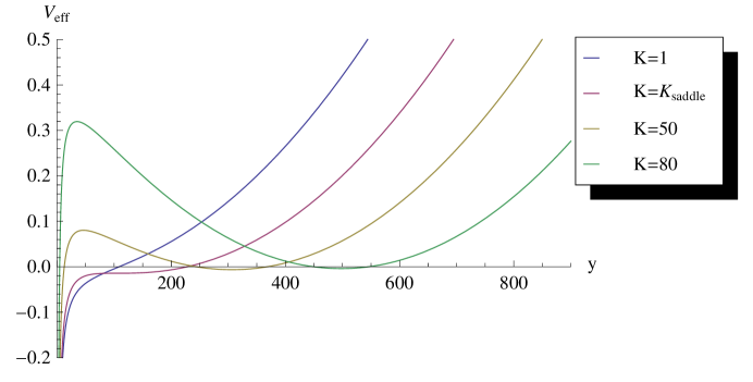
Figure 2: $He^{+}$ ion: effective potential $V_{eff}$ (16) at $K=1,K_{saddle},50,80$. $K_{saddle}\approx 25.13$ and $B=B_{0}=3.7598\times 10^{10}\,G$ . (c.f. ET-genq:2013 )

Since we are going to use an approximate method for solving the Schrödinger equation with the Hamiltonian (14), a quality of the approximation of ground state function can depend on the gauge. In particular, one can ask whether one can find a gauge for which a given trial function leads to minimal variational energy. Such a gauge (if found) can be called optimal for a chosen trial function.

To this end, it is convenient to introduce a gauge transformation

$${U}\ =\ e^{i\,B\,q_{\rm{w}}\,(1-\xi)(1-\nu)\,{y}_{0}\,x}\ ,$$ (22)

where

$${y}_{0}=-\frac{d\,K}{e\,\mu\,B}$$ (23)

and $\nu,\,d$ are parameters. The gauge transformed Hamiltonian (14) takes the form

$${h}_{d,\,\nu}\ \equiv\ U^{-1}\,{h}\,U\ = \ \frac{(-\partial^{2}_{{}_{Y}}-2\,i\,B\,e\,\mu\,x\,\partial_{{}_{Y}}+e^{2}\,B^{2}\,Y^{2}+2\,e\,B\,Y\,(K-B\,e\,\mu\,y))}{2\,M}$$ (24)

$$\ +\frac{{({\mathbf{\hat{p}}}-q_{\text{w}}\,{\mathbf{A}_{(\boldsymbol{\rho}-{\boldsymbol{\rho}}_{0})}})}^{2}}{2\,m_{r}}+V_{eff}\ ,$$

where ${\boldsymbol{\rho}}_{0}=y_{0}(1-\nu)\,\hat{\mathbf{y}}$. This transformation implies that we consider now the Schrödinger equation in a linear gauge for which the position of the gauge center, where $\mathbf{A}(x,y)=0$, is located at

$$x=0\,,\quad y=\frac{d\,K}{e\,\mu\,B}(1-\nu)\ .$$ (25)

For $K>K_{saddle}$ we expect the gauge center to be localized on the line $x=0$, between the origin $y=0$ and the second minimum $y=y_{0,min}$ of $V_{eff}$, (see (19)). Thus, the vector potential can be considered as a variational function and can be chosen by a procedure of minimization as it was proposed in PRepts and realized in ET-genq:2013 (see also for discussion Vincke ). For a moving neutral system, the case $d=0$ has been used in the past to study the so-called centered states with wavefunction peaked at the Coulomb minimum Burkova . While for the so-called ”decentered” states it seems natural to consider $d=1$. The eigenvalue problem

$${h}_{d,\nu}\,\chi_{{}_{K}}=E\,\chi_{{}_{K}}\ ,$$ (26)

where $\chi_{{}_{K}}(\boldsymbol{\rho},\,Y)\ =\ e^{-i\,B\,q_{\rm{w}}\,(1-\xi)(1-\nu)\,{y}_{0}\,x}\,\psi_{{}_{K}}(\boldsymbol{\rho},\,Y)$, is the central object of our study hereafter. For convenience, in the calculations we used the so called shifted representation, $\chi_{{}_{K}}(\boldsymbol{\rho},\,Y)\rightarrow\chi_{{}_{K}}(\boldsymbol{\rho}+y_{0}\,\hat{\mathbf{y}},\,Y)$.

II.1 Asymptotics.

If we put $\chi_{{}_{K}}=\text{e}^{-\varphi}$ and $\xi=\frac{1}{2}$ in (26), one can construct the WKB-expansion at large $\rho=\sqrt{x^{2}+y^{2}}$ for the phase $\varphi$. The leading term at $\rho\rightarrow\infty$ is given by

$$\varphi\ =\ \frac{B}{2}{\bigg{(}\frac{m_{r}}{M}e^{2}\,\mu^{2}+\frac{q_{\rm{w}}^{2}}{4}\bigg{)}}^{\frac{1}{2}}\,\rho^{2}+O(\rho)\ .$$ (27)

Similarly, at $Y\rightarrow\infty$

$$\varphi\ =\ \frac{e\,B}{2}\,Y^{2}+O(Y)\ .$$ (28)

In the limit $\rho\rightarrow 0$ we obtain

$$\varphi\ =\ -4\,m_{r}\,e^{2}\,\rho+O(\rho^{2})\ .$$ (29)

Assuming the condition (18) is fulfilled, the potential (16) has the second minimum at $y_{0,min}\neq 0$. Hence, the double Taylor expansion of the phase at $x=0,y=y_{0,min}$ has the form

$$\varphi \ =\ \alpha_{0}+\alpha_{2}\,{(y-y_{0,min})}^{2}+\alpha_{3}\,{(y-y_{0,min})}^{3}+\alpha_{4}\,{(y-y_{0,min})}^{4}+\ldots$$ (30)

$$\ +\beta_{2}\,x^{2}+\beta_{4}\,x^{4}+\ldots+\gamma_{3}\,(y-y_{0,min})\,x^{2}+\ldots$$

where $\alpha$’s, $\beta$’s and $\gamma$’s are constants.

II.2 Approximations

Following the prescription formulated in Turbiner:1988-2010 we make an interpolation between WKB-expansion (27),(28) and the perturbative expansion (29),(30) and construct a trial function for the ground state of (26) in a form of a product

$$\chi_{{}_{K}}(\boldsymbol{\rho},\,Y)\ =\ e^{-a^{2}\,Y^{2}+b\,Y\,y-\beta^{2}\,y^{2}}\ \zeta(\boldsymbol{\rho})\,\ ,$$ (31)

where

$$\zeta(\boldsymbol{\rho})\ =\ C_{1}\,e^{-\phi_{c}}+C_{2}\,e^{-\phi_{m}}$$ (32)

$$\phi_{c}=\ \frac{A_{0}+A_{1}\,{\rho}+A_{2}\,{y}\,{\rho}+A_{3}^{2}\,{\rho^{3}}}{\sqrt{1+A_{4}\,{y}+A_{5}^{2}\,{\rho^{2}}}}-\frac{\alpha}{2}\,\log(1+A_{4}\,{y}+A_{5}^{2}\,{\rho^{2}})$$

$$\phi_{m}=\ \frac{D_{0}+D_{1}\,{{x}^{2}}+D_{2}\,{{\tilde{y}}^{2}}+D_{3}^{2}\,{\varrho^{4}}}{\sqrt{1+D_{4}\,{{x}^{2}}+D_{5}\,{{\tilde{y}}^{2}}+D_{6}^{2}\,{\varrho^{4}}}}$$

with $\tilde{y}=y-y_{0}$, $\varrho^{2}={x}^{2}+{\tilde{y}}^{2}$ and $a,\,b,\,\beta,\,A^{\prime}s,\,C^{\prime}s,D^{\prime}s,\,\alpha$ variational parameters. Supposedly, they should behave smoothly as a function of a magnetic field.

As mentioned above this problem has some similarity with that of the moving neutral system for which a physically adequate trial function is $\zeta(\boldsymbol{\rho})$. The difference comes from the first term in r.h.s. of (14), the contribution of this term is encoded in the factor $e^{-a^{2}\,Y^{2}+b\,Y\,y-\beta^{2}\,y^{2}}$ in (31). The parameter $b$ measures the coupling between CM and relative variables, $b=0$ corresponds to the adiabatic approximation.

III Results

We carried out a variational study of the two-body charged system on a plane moving across a magnetic field. The main emphasis is to explore stability of the system, thus, studying the ground state. For the case of $He^{+}$ ion, the energy for several magnetic fields $0<B<100$ a.u. and values of Pseudomomentum $0\leq K<1000$ a.u. is presented in Table 1. The energy grows monotonically and rather sharp as a function of a magnetic field for fixed Pseudomomentum but at much slow pace as a function of Pseudomomentum for a fixed magnetic field. It is worth noting that for fixed $B$ the energy $E$ as a function of $K$ tends asymptotically to the ground state energy of two non-interacting charges in a magnetic field.

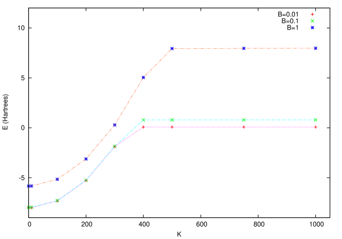
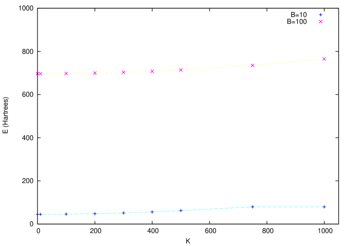
Figure 3: The energy (in Hartrees) of ground state vs Pseudomomentum $K$. (a) $E$ vs $K$ for magnetic fields $B=0.01,\,0.1,\,1$. (b) $E$ vs $K$ for magnetic fields $B=10,\,100$ a.u.; magnetic field $B$ and Pseudomomentum $K$ in effective atomic units, $B_{0}=3.7598\times 10^{10}\,G$. (c.f. ET-genq:2013 Fig. 2)

After making a minimization, one can see the appearance of a sharp change in the behavior of parameters in (32) as a function of $K$. It is related with a fact of the existence of a certain critical Pseudomomentum $K_{c}>K_{saddle}$ such that for $K<K_{c}$ the optimal linear parameters $C_{1}\approx 1,\,C_{2}\approx 0$ the wavefunction has a peak near the Coulomb singularity (centered state). At $K>K_{c}$ the situation gets opposite: the parameters $C_{1}\approx 0,\,C_{2}\approx 1$ and the wavefunction is peaked near the second well of (16), see Fig.2 (we call this well the magnetic well) which corresponds to a decentered state. A similar phenomenon appears in the case of a neutral system in 3D Burkova and 2D Lozovik:2002 . The existence of such a change in the behavior of parameters results also in a specific behavior of energy dependence (see for example Fig.3) and mean interparticle separation vs. the Pseudomomentum. From physical point of view at $K=K_{c}$ the effective depth of the Coulomb well and that of the magnetic well get equal. If $K<K_{c}$ the effective depth of the Coulomb well is larger (or much larger depending on a magnetic field strength) than one of the magnetic well, the system prefers to stay at the Coulomb well. If $K>K_{c}$ the effective depth of the Coulomb well is smaller (or much smaller depending on a magnetic field strength) than one of the magnetic well, the system prefers to stay at the magnetic well. For all studied magnetic fields the barrier between wells is very large, the probability of tunneling from one well to the other is very small. Hence, the energy behavior vs. CM Pseudomomentum $K$ is defined by one well or another, it is close to classical behavior. Thus, the presence of the second minimum in the effective potential can be neglected.

The results of calculations show that the optimal gauge parameter $\xi$ for all values of magnetic field considered always corresponds to symmetric gauge $\xi=\frac{1}{2}$. The behavior of $K_{c}$ as a function of magnetic field is presented in Fig. 4 where $K_{c}$ grows with an increase of $B$. The evolution of the gauge center parameters ($d,\,\nu$), see ((22)-(25)), vs. CM Pseudomomentum $K$ is shown in Tables 2-3, respectively. For $K<K_{c}$ the parameter $d$ is very small, it varies within $[0-5\times 10^{-5}]$ for magnetic field range $0.01-100$ a.u. while for $K>K_{c}$ it is close to 1, it varies within $[1-0.996]$ for magnetic field range $0.01-10$ a.u. At $B<1$ and for any $K$ considered the parameter $\nu\sim 0$. At fixed $B\eqslantgtr 1$ the parameter $\nu=\nu(B)\neq 0$ for $K<K_{c}$ and almost constant for $K\gtrsim K_{c}$. Thus, the gauge as a function of $K$ changes from the symmetric gauge centered at the Coulomb well (the singularity of (16)) to the symmetric gauge but centered at the magnetic well (the minimun of (16) for $K>K_{c}$). In turn, the parameter $d$, which mainly determines the value of the gauge center, remains almost equal to $0$ up to $K=K_{c}$ (which means the gauge center coincides with a position of the Coulomb singularity, then sharply jumps to a value close to $1$ (gauge center coincides with a position of the minimum of magnetic well), displaying a behavior which looks like a phase transition. But it is not a phase transition: the energy changes sharply but smoothly. For $K=K_{c}$ the gauge parameters are $d\sim 0.5,\,\nu\sim 0$. There exists a certain domain of transition from one regime to another. Overall situation looks very similar to that for the $H_{2}^{+}$ molecular ion in a magnetic field in inclined configuration PRepts .

In order to illustrate the transition from a centered state to a decentered one we have calculated, using the trial function (31) with optimal parameters, the expectation value of the relative coordinate $\langle\rho\rangle$, see Table 4. At weak magnetic fields $B$, the transition is very sharp, becoming even more pronounced with a magnetic field decrease. For all studied magnetic fields and Pseudomomentum both $\langle\rho\rangle$ and $\langle Y\rangle$ are finite. Furthermore, the trial function (31) remains normalizable. It indicates the stability and boundedness of the $He^{+}$ ion in magnetic field.

To complete the study we show in Tables VIII - XIV (see Supplementary Materials) the nonlinear parameters $\beta$, $A$’s, $D$’s and $\alpha$ of the trial function (32) as a function of the magnetic field strength for the optimal configuration. For all considered values of Pseudomomentum the parameter $A_{1}\approx 4$. A deviation $|A_{1}-4|$ measures (anti)-screening of the electric charge due to the presence of a magnetic field. The optimal value of energy corresponds to $y_{0}\approx y_{0,min}$. Similarly, for all considered values of Pseudomomentum the parameter $a\approx 0.283,\,0.8943,\,2.828,\,8.942,\,28.277$ at $B=0.01,\,0.1,\,1,\,10,\,100$, respectively. A deviation $|1-\frac{1}{a}\sqrt{\frac{e\,B}{2}}|\lesssim 10^{-4}$ measures the correctness of the asymptotic behavior of the trial function, see (28).

In Table 5 the evolution of parameter $b$ is presented, it shows that the coupling between CM and relative variables is a non-decreasing function of magnetic field. For fixed $B$ the behavior is different, at $K<K_{c}$ the optimal value of $b$ is a decreasing function (changing from a positive value to a negative one) of Pseudomomentum while for $K>K_{c}$ the parameter $b>0$ is almost constant. Because there is no separation of variables in the problem, $b$ is never zero. Clearly, the parameter $b$ will play an important role either for $B\rightarrow\infty$ or for systems with $m_{r}\sim 0.5$.

Our variational results are checked on agreement with results obtained with other methods. We used the Lagrange mesh method (see Baye and references therein) to obtain the ground energy for $B=0.1$ a.u. and different Pseudomomentum $K$, see Table 7. For all studied values of $K$ the variational energy is in agreement with Lagrange mesh calculations in not less than 5 s.d. . It is interesting to check the accuracy of the Born-Oppenheimer approximation (taking $m_{2}\rightarrow\infty$) as well. The results are presented in Table 6. The relative difference in energy due to the finite mass effects are of order $\approx 10^{-4}$ for all $B$, as expected.

$He^{+}$ ion. Energy $E$

$K$	$E$
	$B=0.01$        $B=0.1$        $B=1$        $B=10$        $B=100$
$0$	$-7.9986$	$-7.9690$	$-5.8365$	$45.226$	$696.89$
$10$	$-7.9918$	$-7.9622$	$-5.8297$	$45.232$	$696.90$
$100$	$-7.3184$	$-7.2888$	$-5.1563$	$45.905$	$697.57$
$200$	$-5.2778$	$-5.2482$	$-3.1159$	$47.944$	$699.60$
$300$	$-1.8767$	$-1.8472$	$0.2846$	$51.342$	$702.99$
$400$	$0.07920^{d}$	$0.7920^{d}$	$5.0454$	$56.098$	$707.74$
$500$	$0.07936^{d}$	$0.7936^{d}$	$7.9359^{d}$	$62.214$	$713.84$
$750$	$0.07957^{d}$	$0.7957^{d}$	$7.9573^{d}$	$79.572^{d}$	$735.02$
$1000$	$0.07968^{d}$	$0.7968^{d}$	$7.9680^{d}$	$79.680^{d}$	$764.66$

Table 1: Ground state energy $E$ in Hartrees (see (26)); magnetic field $B$ and Pseudomomentum $K$ in effective atomic units, $B_{0}=3.7598\times 10^{10}$ G. , $K/\hbar=5.5\times 10^{12}\,{\rm cm}^{-1}$, respectively. Energies corresponding to decentered states marked by ^d (see text).

$He^{+}$ ion. Parameter $d$

$K$	$d$
	$B=0.01$       $B=0.1$             $B=1$               $B=10$                   $B=100$
$K<K_{c}$	$0.0$	$0.0$	$-2.0\times 10^{-6}$	$-5\times 10^{-6}$	$5.0\times 10^{-5}$
$K>K_{c}$	$1.0$	$0.9998$	$0.999$	$0.996$	$-$

Table 2: Optimal gauge parameter $d$ (see (25)) for different magnetic fields and pseudomomenta; magnetic field in effective atomic units, $B_{0}=3.7598\times 10^{10}$ G.

$He^{+}$ ion. Parameter $\nu$

$K$	$\nu$
	$B=1$           $B=10$             $B=100$
$0$	$0$	$0$	$0$
$10$	$-27.292$	$-22.121$	$79.715$
$100$	$-131.66$	$-68.226$	$135.59$
$200$	$-305.13$	$-316.21$	$135.60$
$300$	$-638.94$	$-570.81$	$135.79$
$400$	$-638.94$	$-746.60$	$95.506$
$500$	$0$	$-750.29$	$34.637$
$750$	$0$	$0$	$34.527$
$1000$	$0$	$0$	$5.1179$

Table 3: Ground state. Parameter $\nu$ in (25). At $B=0.01,\,0.1$, parameter $\nu\sim 0$ for all $K$ considered. $B_{0}=3.7598\times 10^{10}\,G$.

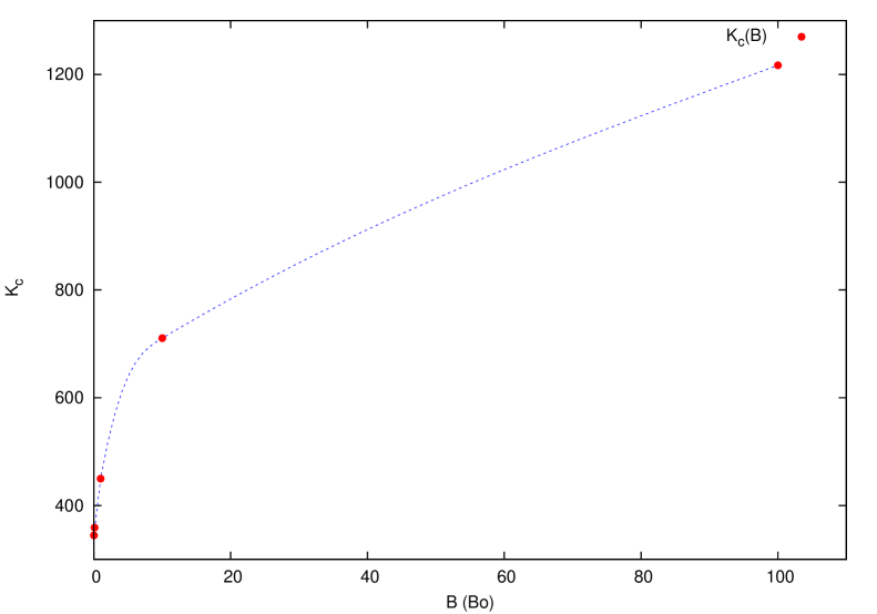
Figure 4: Critical Pseudomomentum $K_{c}$ vs $B$ , (c.f. ET-genq:2013 Fig. 3)

$He^{+}$ ion. Expectation value $\langle\rho\rangle$

$K$	$\langle\rho\rangle$
	$B=0.01$         $B=0.1$         $B=1$
$0$	$0.250$	$0.248$	$0.198$
$100$	$0.250$	$0.248$	$0.198$
$300$	$0.250$	$0.248$	$0.198$
$400$	$2500^{d}$	$249^{d}$	$0.198$
$500$	$3125^{d}$	$312^{d}$	$31^{d}$
$750$	$4688^{d}$	$468^{d}$	$46^{d}$
$1000$	$6250^{d}$	$625^{d}$	$62^{d}$

Table 4: Expectation value $\langle\rho\rangle$; magnetic field in effective atomic units, $B_{0}=3.7598\times 10^{10}\,G$. At $B=10,100$ a.u., $\langle\rho\rangle\approx 0.087,0.018$, respectively. Data corresponding to decentered states marked by ^d  (see text). For $K<K_{c}$, $\langle\rho\rangle\approx 0$, while for $K>K_{c}$, $\langle\rho\rangle\sim\langle y\rangle\sim y_{0,min}\propto K/B$ .

$He^{+}$ ion. Parameter $b$

$K$	$B=1$               $B=10$               $B=100$
	$a=2.828$          $a=8.942$          $a=28.277$
$0$	$0.002$	$0.0349$	$0.4079$
$10$	$0.0019$	$0.0349$	$0.4021$
$100$	$0.0014$	$0.0312$	$0.3983$
$200$	$0.0003$	$0.0299$	$0.3876$
$300$	$-0.0013$	$0.0094$	$0.3475$
$400$	$-0.0040$	$-0.0033$	$0.2973$
$500$	$0.0043^{d}$	$-0.0217$	$0.2395$
$750$	$0.0043^{d}$	$0.0435^{d}$	$0.0371$
$1000$	$0.0043^{d}$	$0.0435^{d}$	$-0.4303$

Table 5: Ground state. Parameters $a,\,b$ in (31). At $B=0.01,\,0.1$, parameter $b\sim 10^{-4}$ and $a=0.283,\,0.8943$ respectively, for all $K$ considered. Data corresponding to decentered states marked by ^d  (see text). $B_{0}=3.7598\times 10^{10}\,G$.

$B$	$E$
	$E_{0}$                   $E_{0}^{\infty}$
$0.01$	$-7.9986$	$-7.9997$
$0.1$	$-7.9690$	$-7.9702$
$1$	$-5.8365$	$-5.8393$
$10$	$45.226$	$45.203$
$100$	$696.89$	$696.67$

Table 6: Ground state energy in Hartrees. $E_{0}$ from Table 1 and $E_{0}^{\infty}$ ($m_{2}\rightarrow\infty$). Magnetic field in effective atomic units, $B_{0}=3.7598\times 10^{10}\,G$ .

$K$	$E$
	$E_{0}$                         $E^{mesh}_{0}$
$0$	$-7.969046$	$-7.969047$
$10$	$-7.962244$	$-7.962245$
$100$	$-7.288839$	$-7.288839$
$300$	$-1.847176$	$-1.847177$
$500$	$0.793600$	$0.793600$
$1000$	$0.796800$	$0.796800$

Table 7: Ground state energy at $B=\frac{1}{10}$. $E_{0}$ from the present study and $E_{0}^{mesh}$ obtained with the Lagrange mesh method (parameters $d,\nu$ taken from the corresponding variational results based on (31)). Magnetic field in effective atomic units, $B_{0}=3.7598\times 10^{10}\,G$.

IV Conclusions

Summarizing, for the two-dimensional $He^{+}$ ion in a constant magnetic field partial factorization of eigenfunctions (see (13)) allows us to reduce the problem to one with three degrees of freedom. For this reduced problem we want to state that a simple uniform approximation of the ground state eigenfunction is constructed. It manifests an approximate solution of the problem. The key element of the procedure is to make an interpolation between the WKB expansion at large distances and perturbation series at small distances both for the phase of the wavefunction; in other words, to find an approximate solution for the corresponding eikonal equation. In general, the separation of variables helps us to solve this problem easily. In our case of non-separability of variables the WKB expansion of a solution of the eikonal equation cannot be constructed in a unified way, since it depends on the way how we approach to infinity. However, a reasonable approximation of the first dominant growing terms of the WKB expansion of the phase seems sufficient to construct the interpolation between large and small distances giving rather high accuracy results.

It was demonstrated that for all magnetic fields and all values of Pseudomomentum the system is bounded. Its energy grows with magnetic field strength increase as well as Pseudomomentum increase. For fixed magnetic field $B$, the energy behavior demonstrates a sharp change for a certain value of CM Pseudomomentum $K_{c}(B)$. It seems it can be used to measure the magnetic field strength. This effect was already mentioned in three-dimensional Hydrogen atom moving across magnetic field Potekhin .

In the Born-Oppenheimer approximation ($m_{2}\rightarrow\infty$), a curious fact that the Hamiltonian (11) possesses the hidden algebra $sl_{2}(\Re)$ is worth mentioning. It can be immediately seen-making a gauge rotation of the Hamiltonian (11) in symmetric gauge ($\xi=\frac{1}{2}$) with the gauge factor $e^{-\frac{e\,B}{4}\rho_{1}^{2}}$ . We obtain the operator which is in the universal enveloping algebra of $sl_{2}(\Re)$ (see e.g. Turbiner:1994 ). Hence, for specific values of a magnetic field $B$ the algebra $sl_{2}(\Re)$ appears in finite-dimensional representation and the problem admits analytical solutions (details will be given elsewhere).

References

• (1) D. Pinheiro and R.S. Mackay,
Interaction of two charges in a uniform magnetic field I: planar case,
Nonlinearity 19 (2006) 1713 - 1745
• (2) M.A. Escobar-Ruiz and A.V. Turbiner,
Two charges on a plane in a magnetic field: special trajectories
Journal of Math Physics
54, 022901 (2013)
• (3) A.V. Turbiner and M.A. Escobar-Ruiz,
Two charges on a plane in a magnetic field: hidden algebra, (particular) integrability, polynomial eigenfunctions,
J. Phys. A: 46 , 295204 (2013)
• (4) M. Taut,
Two electrons in a homogeneous magnetic field: particular analytical solutions,
J. Phys. A27, 1045 (1994)
• (5) M. Taut,
Two particles with opposite charge in a homogeneous magnetic field: particular analytical solutions of the two-dimensional Schrödinger equation,
J. Phys. A32 (1999) 5509 - 5515
• (6) A.V. Turbiner,
Two electrons in an external oscillator potential: The hidden algebraic structure
Phys. Rev. A
50, 5335 (1994)
• (7) R. H. Garstang,
Atoms in high magnetic fields (white dwarfs),
Rep. Prog. Phys. 40 40 (1977) 105
• (8) J.E. Avron, I.W. Herbst and B. Simon,
Separation of centre of mass in homogeneous magnetic fields,
Ann. Phys. 114 (1978) 431
• (9) Victor G. Bezchastnov, George G. Pavlov and Joseph Ventura
Discrete eigenstates of the $He^{+}$ ion moving in a strong magnetic field,
Phys. Rev. A 58 (1998)
• (10) A.V. Turbiner,
Particular integrability and (quasi)-exact-solvability
J. Phys. A:
46 , 025203 (2013)
• (11) L.P. Gorkov, I.E. Dzyaloshinskii,
Contribution to the Theory of the Mott Exciton in a Strong Magnetic Field,
ZhETF 53 (1967) 717-722;
Sov. Phys. JETP 26 (1968) 449-451 (English translation)
• (12) M.A. Escobar-Ruiz and A.V. Turbiner,