Variational description of the ground state of the repulsive two-dimensional Hubbard model in terms of nonorthogonal symmetry-projected Slater determinants

Abstract

The few determinant (FED) methodology, introduced in our previous works [Phys. Rev. B 87, 235129 (2013) and Phys. Rev. B 89, 195109 (2014)] for one-dimensional (1D) lattices, is here adapted for the repulsive two-dimensional Hubbard model at half-filling and with finite doping fractions. Within this configuration mixing scheme, a given ground state with well defined spin and space group quantum numbers, is expanded in terms of a nonorthogonal symmetry-projected basis determined through chains of variation-after-projection calculations. The results obtained for the ground state and correlation energies of half-filled and doped 4 $\times$ 4, 6 $\times$ 6, 8 $\times$ 8, and 10 $\times$ 10 lattices, as well as momentum distributions and spin-spin correlation functions in small lattices, compare well with those obtained using other state-of-the-art approximations. The structure of the intrinsic determinants resulting from the variational strategy is interpreted in terms of defects that encode information on the basic units of quantum fluctuations in the considered 2D systems. The varying nature of the underlying quantum fluctuations, reflected in a transition to a stripe regime for increasing onsite repulsions, is discussed using the intrinsic determinants belonging to a 16 $\times$ 4 lattice with 56 electrons. Such a transition is further illustrated by computing spin-spin and charge-charge correlation functions with the corresponding multireference FED wave functions. In good agreement with previous studies, the analysis of the pairing correlation functions reveals a weak enhancement of the extended $s$-wave and d${}_{x^{2}-y^{2}}$ pairing modes. Given the quality of results here reported together with those previously obtained for 1D lattices and the parallelization properties of the FED scheme, we believe that symmetry projection techniques are very well suited for building ground state wave functions of correlated electronic systems, regardless of their dimensionality.

I Introduction.

Due to its challenging complexity, the description of low-dimensional correlated electronic systems still represents an open problem in condensed matter physics. Dagotto-review ; Dagotto-Rev-Mod-Physics-2013 In particular, their quantum correlation effects can exhibit unconventional features. A typical example, is the spin-charge separation text-Hubbard-1D ; Voit ; Ogata-Shiba in the strong interaction regime of the one-dimensional (1D) Hubbard model. Hubbard-model_def1 ; Gebhard-1 Angle-resolved photoemision spectroscopy studies also reveal a complex pattern of spin-charge coupling/decoupling in both the 1D and two-dimensional (2D) cases in the weak and intermediate-to-strong interaction regimes. Kim ; KMShen How to account for these, and many more, quantum correlation effects in the simplest possible way has become a driving force for developing theoretical approximations that could complement already existing state-of-the-art methods like exact diagonalization Dagotto-review ; Lanczos-Fano (ED), quantum (QMC) and variational (VMC) Monte Carlo, Raedt-MC ; Nightingale ; Shiwei-QMC-Symmetry ; Neuscamman-2012 coupled cluster, Bishop-1 ; Bishop-2 variational reduced-density-matrix, Hammond density matrix renormalization group, DMRG-White ; Scholl-RMP matrix product and tensor network states, Scholl-AP ; GChan ; TNPS-1 ; TNPS-2 ; Vidal as well as quantum embedding approaches. Zgid ; maier2005 ; stanescu2006 ; DMFT-1 ; moukouri2001 ; huscroft2001 ; aryanpour2003 ; DVP-2 ; Knizia-Chan ; Irek-DMET-paper1 ; Irek-DMET-paper2 ; DMET-honey All these methods have already been applied to Hubbard-like 1D and/or 2D models with variable degree of success.

The exact Bethe-ansatz solution to the 1D Hubbard model is well known. BETHE ; LIEB Because of this, the model has been frequently used as a testing ground for several theoretical frameworks. However, an intuitive physical picture of the basic units of quantum fluctuations in the considered 1D systems has remained an open issue within several approximations. In recent years, both single reference (SR) and multireference (MR) symmetry-projected approximations, Tomita-1 ; Tomita-2 ; Tomita-3 ; Tomita-2011PRB ; Carlos-Hubbard-1D ; Rayner-2D-Hubbard-PRB-2012 ; non-unitary-paper-Carlos ; rayner-Hubbard-1D-FED2013 ; rayner-Hubbard-1D-FED2014 ; Carlos-Rayner-Gustavo-VAMPIR-molecules ; Carlos-Rayner-Gustavo-FED-molecules ; Laimis-paper ; PQT-reference-1 ; PQT-reference-2 ; PQT-reference-3 ; Juillet routinely used in nuclear structure physics, rs ; Carlo-review ; Schmid-Gruemmer-1984 ; Rayner-Carlo-CM-1 ; Rayner-Carlo-CM-2 ; rayner-GCM-paper ; rayner-GCM-parity have been applied to describe correlated electronic systems. It has been shown that MR schemes like the Resonating Hartree-Fock Tomita-1 ; Tomita-2 ; Tomita-3 ; Tomita-2011PRB ; Fukutome-original-RSHF ; Yamamoto-1 ; Yamamoto-2 ; Ikawa-1993 (ResHF) and the Few Determinant Carlo-review ; Schmid-Gruemmer-1984 ; rayner-Hubbard-1D-FED2013 ; rayner-Hubbard-1D-FED2014 ; Carlos-Rayner-Gustavo-VAMPIR-molecules ; Carlos-Rayner-Gustavo-FED-molecules (FED) ones, provide a reasonable description of the ground state energies of half-filled and doped 1D Hubbard lattices but also account for the main physical trends in correlation functions, momentum distributions, spectral functions, and density of states. Tomita-1 ; rayner-Hubbard-1D-FED2013 ; rayner-Hubbard-1D-FED2014 In addition, within these approaches, one is left with a simple physical picture in which the basic units of quantum fluctuations in 1D lattices can be mainly associated with structural defects in the (intrinsic) Slater determinants resulting from the corresponding optimizations. Tomita-1 ; rayner-Hubbard-1D-FED2013 ; rayner-Hubbard-1D-FED2014

The situation is more involved in the case of the 2D Hubbard model for which no general (exact) solution is known. Such a model has received considerable attention since the discovery of high-T_C superconductors HTCSC-1 and has also become the target for theorists applying many-body methodologies. According to Anderson’s proposal, Anderson-1 2D Hubbard is considered a potential model for describing the essential physics in the cuprates. With intensive analytic and numerical studies, Theory-strong some aspects of the phase diagram have been understood. Dagotto-review However, many basic features remain controversial. For example, while it is accepted that the onsite interaction strength drives a Mott transition to an insulator at half-filling, Hirsch-1 ; Hirsch-2 ; White-AF-HF ; Furukawa it is much more difficult to accurately describe what happens to the antiferromagnetic order when the system is doped.

From the experimental point of view, cold atoms in optical lattices offer potential direct simulations of Hubbard-like models. optical-1 On the other hand, such models are valuable tools to study the properties of graphene CastroNeto-review and their (multiorbital) extensions Su-Fe-Dagotto have already provided insight into the interplay between electronic correlations and doping in the parent states of high-T_C iron-based superconductors. sup-Fe ; Stewart-Review Futhermore, both the colossal magnetic resistance and large thermopower has attracted considerable attention. Science-Dagotto ; Otha In addition, a fascinating effort to understand exotic spin liquid phases in the ground and low-lying excited states of some 2D systems is bringing new light into the complexity of the associated many-electron problems and the theoretical tools used in their description. SL-1 ; SL-2 ; SL-3 We believe that the previous examples illustrate the need to explore new avenues for describing quantum correlation effects in low-dimensional electronic systems, especially those approximations that are potentially not restricted by the dimensionality of the considered lattices.

The 2D Hubbard model has already been considered with symmetry projection tools in a previous work Rayner-2D-Hubbard-PRB-2012 using a variation-after-projection (VAP) approach. rs For the considered lattices, it has been shown that such an approach accurately describes both ground and low-lying excited states, with well defined quantum numbers, on an equal footing. The comparison with other state-of-the-art approximations revealed that the method does account for the most relevant correlations including a basic quantum mechanical fingerprint as the low-lying spectrum of the 6 $\times$ 6 lattice, which is out of reach of ED calculations. Symmetry-projected methods also provide a well-controlled ansatz to compute both spectral functions and density of states. However, despite being more sophisticated than SR methods, Carlos-Hubbard-1D ; PQT-reference-1 ; PQT-reference-2 ; PQT-reference-3 ; Juillet our scheme still essentially relied on the description of a given ground and/or excited state in terms of a single symmetry-projected configuration (or component). This certainly limits the amount of correlations that can be described in the ground and excited states of nuclear, Carlo-review condensed mater, Rayner-2D-Hubbard-PRB-2012 and quantum chemistry systems. Carlos-Rayner-Gustavo-VAMPIR-molecules In this study, we present results that go beyond such a single configuration and benchmark a MR method, i.e., the FED approach, rayner-Hubbard-1D-FED2013 further including the breaking and restoration of the full space group symmetry, which was not included in our previous work.

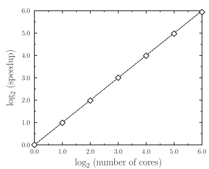
Figure 1: Speedup of a typical UHF-FED calculation for a half-filled 12 $\times$ 12 lattice at U=4t. The origin of the plot refers to a calculation with 1024 cores. The largest calculation uses 65,536 processors. All calculations have been performed at the Titan computational facility, Oak Ridge National Laboratory, Center for Computational Sciences.

The key idea of the FED approach Carlo-review ; rayner-Hubbard-1D-FED2013 ; rayner-Hubbard-1D-FED2014 ; Carlos-Rayner-Gustavo-FED-molecules is to consider a set of symmetry-broken Hartree-Fock (HF) states $|{\cal{D}}^{i}\rangle$ which are used to build, via chains of Ritz-variational calculations, Blaizot-Ripka a correlated nonorthogonal basis of $n$ symmetry-projected configurations $\hat{P}^{\Theta}|{\cal{D}}^{i}\rangle$, with $\hat{P}^{\Theta}$ being a projection operator (see, Sec. II) characterized by the quantum numbers $\Theta$ associated with the irreducible representations of the symmetry groups under consideration. The FED wave function is simply a variationally optimized expansion in terms of these $n$ symmetry-projected states. Let us stress that FED is a VAP scheme, within which the intrinsic states $|{\cal{D}}^{i}\rangle$ are always optimized in the presence of the projection operator $\hat{P}^{\Theta}$. This is what brings a different structure (i.e., defects) in each of the determinants $|{\cal{D}}^{i}\rangle$ as compared with the standard HF ones. StuberPaldus ; HFclassification These intrinsic states $|{\cal{D}}^{i}\rangle$ are optimized one-at-a-time within the FED approach. rayner-Hubbard-1D-FED2013 A simultaneous optimization of all the transformations ${\cal{D}}^{i}$ can become quite demanding in situations where large expansions in terms of nonorthogonal symmetry-projected configurations are required. rayner-Hubbard-1D-FED2014 In fact, it is the FED VAP strategy what allows us to reach expansions larger than those possible within the ResHF scheme, as well as to alleviate our numerical effort in calculations based on the most general HF intrinsic states that require full three-dimensional spin projection. The reason for this is quite simple: in a ResHF optimization ${\cal{O}}(n^{2})$ Hamiltonian and norm kernels have to be recomputed at every iteration while only ${\cal{O}}(n)$ kernels are required in an efficient implementation of FED. Note, however, that we keep the acronym FED just to remain consistent with the literature; there is no need for the FED expansion to be short, as its name would imply, although it is certainly a desirable feature. Even in the case of a SR expansion (i.e., $n=1$), the wave function is, via the projection operator $\hat{P}^{\Theta}$, already multideterminantal in nature, Rayner-2D-Hubbard-PRB-2012 making it a high-quality trial state for the constrained-path QMC (CPQMC) approximation. PaperwithShiwei Last but not least, small vibrations around symmetry-projected mean-fields (i.e., symmetry-projected Tamm-Dancoff and random phase approximations) can be consistently formulated both at the SR and MR levels. RPA-Schmid ; RPA-Nishiyama Such an approximation has been recently used to access a large number of excited states required to compute optical conductivity in lattice models. opticalCon-1 ; opticalCon-2 ; opticalCon-3 Results will be presented in a forthcoming publication. RPA-Rayner

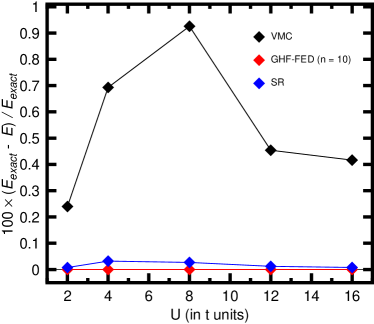
Figure 2: Relative energy errors obtained with the GHF-FED approach based on $n=10$ transformations (red diamonds) are compared with the ones obtained within SR calculations (blue diamonds) as well as with VMC results based on a CPS-Pfaffian ansatz Neuscamman-2012 (black diamonds). Results are shown for a half-filled 4 $\times$ 4 lattice and onsite interactions of U=2t, 4t, 8t, 12t and 16t. For more details, see the main text.

In this paper we adapt the FED methodology, introduced in our previous studies of 1D Hubbard lattices, rayner-Hubbard-1D-FED2013 ; rayner-Hubbard-1D-FED2014 to the half-filled and doped 2D Hubbard model. Our main goal here is not to be exhaustive but rather to test the method’s performance via benchmark calculations on a selected set of illustrative examples. It will be shown below that the FED approach provides accurate correlated ground state wave functions with well defined quantum numbers for 2D systems. For completeness, we briefly describe the key ingredients of our MR approach and set our notation in Sec. II. For a more detailed account, the reader is referred to our previous work. rayner-Hubbard-1D-FED2013 We also illustrate the computational performance of our scheme. Our calculations are discussed in Sec. III. In Sec. III.1, we compare ground state and correlation energies with those obtained using other state-of-the-art approaches. We demonstrate the feasibility of FED calculations on half-filled and doped 2D lattices with 16, 36, 64, and 100 sites. Most of the calculations have been carried out for onsite interactions U=2t, 4t, 8t, and 12t, taken as representatives of the weak, intermediate-to-strong, and strong interaction regimes, respectively. We also discuss the dependence of the predicted correlation energies on the number of basis states used in the corresponding FED expansions, as well as the structure of the intrinsic determinants resulting from the VAP procedure. Having discussed the energetic quality of our states, we turn our attention in Sec. III.2 to momentum distributions and correlation functions. There, we first calibrate the quality of our results in a small 4 $\times$ 4 lattice with N_e=14 electrons. Subsequently, we consider the momentum distribution, spin-spin (SSCF), charge-charge (CCCF) and pairing (PCF) correlation functions in the case of a 16 $\times$ 4 lattice with N_e=56 electrons. We show how for increasing U values our MR ansatz captures the transition to the stripe regime predicted with other theoretical tools. Finally, Sec. IV is devoted to concluding remarks and work perspectives.

II Theoretical framework

We consider the following one-band version of the 2D Hubbard Hamiltonian Hubbard-model_def1 ; Gebhard-1

$$\hat{H}=-t\sum_{{\bf{j}},\sigma}\Big{\{}\hat{c}_{{\bf{j}}+{\bf{x}}\sigma}^{\dagger}\hat{c}_{{\bf{j}}\sigma}+\hat{c}_{{\bf{j}}+{\bf{y}}\sigma}^{\dagger}\hat{c}_{{\bf{j}}\sigma}+h.c\Big{\}}+U\sum_{{\bf{j}}}\hat{n}_{{\bf{j}}\uparrow}\hat{n}_{{\bf{j}}\downarrow}$$ (1)

where the first term represents nearest-neighbor hopping (t $>$ 0) with hopping vectors ${\bf{x}}$=(1,0) and ${\bf{y}}$=(0,1), and the second term is the onsite interaction. In this work, we concentrate on the repulsive sector of the Hubbard model, i.e., U $>$ 0. The fermionic operators $\hat{c}_{{\bf{j}}\sigma}^{\dagger}$ and $\hat{c}_{{\bf{j}}\sigma}$ create and destroy an electron with spin-projection $\sigma=\pm 1/2$ (also denoted as $\sigma=\uparrow,\downarrow$) along an arbitrary chosen quantization axis on a lattice site ${\bf{j}}$=(j_x,j_y). The operators $\hat{n}_{{\bf{j}}\sigma}$ = $\hat{c}_{{\bf{j}}\sigma}^{\dagger}\hat{c}_{{\bf{j}}\sigma}$ are the local number operators. Here, and in what follows, the lattice indices run as j_x=1, $\dots$, N_x and j_y=1, $\dots$, N_y with N_x and N_y being the number of sites along the x and y directions, respectively. We assume periodic boundary conditions along both directions as well as a lattice spacing $\Delta$=1.

Table 1: Ground state energies per site (in t units) obtained with the GHF-FED scheme based on n nonorthogonal symmetry-projected configurations [Eq.(2)] for the 4 $\times$ 4 lattice at different doping fractions and U=4t, 8t and 12t are compared with those obtained within the constrained-path (CPQMC) and release-constraint (RCQMC) QMC approaches, based on trial CASSCF wave functions with symmetries, as well as with those obtained via exact diagonalization (ED) calculations. Shiwei-QMC-Symmetry For each configuration the corresponding set of symmetry quantum numbers $\Theta$ [in all cases ${\bf{k}}$=(0,0)] is also given in the table. For more details, see the main text.

$U/t$		$N_{e}$				$\Theta$						CPQMC				RCQMC				GHF-FED[n]			ED
4		4				1B1						-0.72094(1)				-0.72063(1)				-0.72064[n=1]			-0.72064
8		4				1B1						-0.7082(1)				-0.7075(2)				-0.7076[n=1]			-0.7076
12		4				1B1						-0.7010(1)				-0.7002(3)				-0.7003[n=1]			-0.7003
4		8				1B1						-1.09693(2)				-1.09597(6)				-1.09591[n=10]			-1.09593
8		8				1B1						-1.0307(1)				-1.0282(2)				-1.0288[n=20]			-1.0288
12		8				1B1						-0.9962(1)				-0.9940(3)				-0.9939[n=10]			-0.9941
4		10				1A1						-1.22368(2)				-1.22380(4)				-1.22380[n=20]			-1.22381
8		10				1A1						-1.0948(1)				-1.0942(2)				-1.0942[n=10]			-1.0944
12		10				1A1						-1.0292(1)				-1.0278(4)				-1.0283[n=40]			-1.0284
4		12				1B1						-1.1104(1)				-1.1084(2)				-1.1081[n=30]			-1.1081
8		12				1A1						-0.9376(1)				-0.9329(5)				-0.9327[n=35]			-0.9328
12		12				1A1						-0.8557(1)				-0.8507(6)				-0.8509[n=30]			-0.8512
4		14				1B1						-0.9863(1)				-0.9840(1)				-0.9840[n=20]			-0.9840
8		14				1B1						-0.7461(1)				-0.7417(8)				-0.7417[n=40]			-0.7418
12		14				1B1						-0.6296(2)				-0.627(4)				-0.6281[n=30]			-0.6282
4		16				1A1						-0.85140(6)				-0.85133(6)				-0.85134[n=10]			-0.85137
8		16				1A1						-0.5293(2)				-0.5291(2)				-0.5293[n=10]			-0.5293
12		16				1A1						-0.3741(2)				-0.3739(4)				-0.3745[n=10]			-0.3745

Within the FED approach, rayner-Hubbard-1D-FED2013 ; rayner-Hubbard-1D-FED2014 we consider a set of spin and space group symmetry-broken HF determinants $|{\cal{D}}^{i}\rangle$ ($i=1,\dots$, n). Each of these determinants $|{\cal{D}}^{i}\rangle$ is a convenient mean field (intrinsic) trial configuration. We restore the symmetries of the 2D Hubbard Hamiltonian Eq.(1). resorting to projection techniques. rs ; Carlo-review ; Schmid-Gruemmer-1984 Let us denote $R(\Omega)$ and $\hat{R}(g)$ as the symmetry operations associated with the spin and space groups, respectively, parametrized in terms of the Euler angles $\Omega$=$(\alpha,\beta,\gamma)$ and the label g for the corresponding point group operations. One then uses the degeneracy of the Goldstone states $|{\cal{D}}^{i}(\Omega,g)\rangle=\hat{R}(\Omega)\hat{R}(g)|{\cal{D}}^{i}\rangle$ to recover the desired global gauge symmetries by means of a MR FED wave function of the form

$$|\phi_{K}^{\Theta}\rangle=\sum_{K^{{}^{\prime}}}\sum_{i=1}^{n}f_{K^{{}^{\prime}}}^{i\Theta}\hat{P}_{KK^{{}^{\prime}}}^{\Theta}|{\cal{D}}^{i}\rangle$$ (2)

which expands a given ground state $|\phi_{K}^{\Theta}\rangle$, with well defined spin and space group quantum numbers $\Theta$, in terms of n nonorthogonal symmetry-projected basis states. The operator $\hat{P}_{KK^{{}^{\prime}}}^{\Theta}$ takes the form

$$\hat{P}_{KK^{{}^{\prime}}}^{\Theta}=\frac{h}{L}\sum_{m}^{L}{\Gamma}_{KK^{{}^{\prime}}}^{\Theta*}(m)\hat{R}(m)$$ (3)

where the sum runs over all the symmetry transformations realized by $\hat{R}(\Omega,g)$.

The quantity ${\Gamma}_{KK^{{}^{\prime}}}^{\Theta}(m)$ represents the character of the irreducible representation Edmonds ; Tomita-1 ; Lanczos-Fano while h and L are the dimension of the irreducible representation and the order of the corresponding symmetry group, respectively. In the case of the continuous SU(2) spin-rotational symmetry, the sum should be understood as a group integration with the appropriate measure. Edmonds

Table 2: Ground state energies (in t units) obtained with the CPQMC approach based on SR symmetry-projected UHF (SR-UHF-CPQMC) and GHF (SR-GHF-CPQMC) states PaperwithShiwei are compared with those obtained with MR UHF-FED and GHF-FED calculations, based on n transformations, in the case of a 4 $\times$ 4 lattice with 12 and 14 electrons at U=4t and 8t. For each configuration the corresponding set of symmetry quantum numbers $\Theta$ [in all cases ${\bf{k}}$=(0,0)] is included in the table. Exact diagonalization (ED) results Shiwei-QMC-Symmetry ; PaperwithShiwei are listed in the last column. For more details, see the main text.

$U/t$		$N_{e}$				$\Theta$						UHF-CPQMC				UHF-FED[n]				GHF-CPQMC				GHF-FED[n]			ED
4		12				1B1						-17.7327(8)				-17.7293[n=130]				-17.7301(1)				-17.7296[n=30]			-17.7296
8		12				1A1						-14.914(3)				-14.9227[n=160]				-14.920(1)				-14.9232[n=35]			-14.925
4		14				1B1						-15.7482(5)				-15.7422[n=50]				-15.7455(2)				-15.7440 [n=20]			-15.7446
8		14				1B1						-11.872(3)				-11.8665[n=130]				-11.847(3)				-11.8672[n=40]			-11.8688

The linear momenta $k_{x}=\frac{2\pi}{N_{x}}$ ${\xi}_{x}$ and $k_{y}=\frac{2\pi}{N_{y}}$ ${\xi}_{y}$ are given in terms of the quantum numbers ${\xi}_{x}$ and ${\xi}_{y}$ which take the values allowed inside the Brillouin zone. Ashcroft-Mermin-book Obviously, since we consider the full space group, for certain high symmetry momenta, additional parities $b_{x}$, $b_{y}$ and $b_{xy}$ under x, y and x-y reflections are needed. For example, in the case of a square lattice we refer to states with $\Theta=(0,0,0,+1,+1,+1)$ and $\Theta=(0,0,0,+1,+1,-1)$ as ¹A₁ and ¹B₁ configurations, respectively, with ${\bf{k}}$=(0,0). For the sake of brevity, we refer to these states in what follows as ¹A₁ and/or ¹B₁ configurations . However, the reader should keep in mind that we always use the full set of quantum numbers required to characterize a given FED state.

In this study, we have considered two types StuberPaldus ; HFclassification of intrinsic Slater determinants $|{\cal{D}}^{i}\rangle$ in the expansion Eq.(2), i.e., unrestricted (UHF) and generalized (GHF) Hartree-Fock :

• UHF states preserve $\hat{S}_{z}$-symmetry while possibly breaking all others. They preserve N_e,↑ and N_e,↓ electron number.

• GHF states break all Hubbard 2D Hamiltonian symmetries and can only be characterized by N_e, the total number of electrons.

In those cases where calculations are performed in terms of symmetry-projected UHF configurations, the integrals in both Euler angles $\alpha$ and $\gamma$, associated with the spin-projection operator, become trivial and can be carried out analytically. Calculations in terms of symmetry-projected GHF states are more elaborate as they necessitate numerical integrations over a three-dimensional $(\alpha,\beta,\gamma)$-grid. To indicate the type of Slater determinants used, we refer to the corresponding VAP calculations as UHF-FED and GHF-FED, respectively. Obviously, for the same number n of transformations, a GHF-FED ansatz is computationally more demanding but also accounts for more correlations than the UHF-FED one, because of its larger variational flexibility. However, given the fact that UHF-FED calculations are roughly two orders of magnitude less computationally demanding than GHF-FED, in this study we have also resorted to the former. This alleviates our numerical effort and enable us to reach larger lattices and/or a larger number n of basis states in Eq.(2).

Regardless of the UHF or GHF symmetry-broken character of the $|{\cal{D}}^{i}\rangle$ states used, the MR FED wave function $|\phi_{K}^{\Theta}\rangle$ is determined applying the variational principle to the projected energy

$$E^{\Theta}=\frac{f^{\Theta\dagger}{\cal{H}}^{\Theta}f^{\Theta}}{f^{\Theta\dagger}{\cal{N}}^{\Theta}f^{\Theta}}$$ (4)

written in terms of the Hamiltonian and norm overlaps

$${\cal{H}}_{iK,jK^{{}^{\prime}}}^{\Theta} = \langle{\cal{D}}^{i}|\hat{H}\hat{P}_{KK^{{}^{\prime}}}^{\Theta}|{\cal{D}}^{j}\rangle$$

$${\cal{N}}_{iK,jK^{{}^{\prime}}}^{\Theta} = \langle{\cal{D}}^{i}|\hat{P}_{KK^{{}^{\prime}}}^{\Theta}|{\cal{D}}^{j}\rangle$$ (5)

between all the symmetry-projected configurations in Eq.(2). All the matrix elements $\langle{\cal{D}}^{i}|\hat{H}\hat{R}(\Omega,g)|{\cal{D}}^{j}\rangle$ and $\langle{\cal{D}}^{i}|\hat{R}(\Omega,g)|{\cal{D}}^{j}\rangle$ needed to compute the kernels Eq.(II) can be found with the help of the extended Wick theorem. Blaizot-Ripka For the mixing coefficients $f^{i\Theta}$ we obtain a resonon-like Gutzwiller_method eigenvalue equation

$$\left({\cal{H}}^{\Theta}-E^{\Theta}{\cal{N}}^{\Theta}\right)f^{\Theta}=0$$ (6)

with the constraint $f^{\Theta\dagger}{\cal{N}}^{\Theta}f^{\Theta}=1$ ensuring the normalization of the wave function. The energy Eq.(4) is varied only with respect to the last added determinant $|{\cal{D}}^{n}\rangle$ keeping all the other transformations ${\cal{D}}^{i}$ (i=1, $\dots$, $n-1$), obtained in previous VAP calculations, fixed. rayner-Hubbard-1D-FED2013 ; Carlo-review ; Carlos-Rayner-Gustavo-FED-molecules We have parametrized the variation with respect to each of the transformations ${\cal{D}}^{i}$ in terms of the Thouless theorem. rs Such a parametrization has already been shown to be a useful tool in nuclear structure Rayner-Robledo-fission-2014 ; Carlo-review ; Rayner-Carlo-CM-1 ; Rayner-Carlo-CM-2 and condensed matter Carlos-Hubbard-1D ; Rayner-2D-Hubbard-PRB-2012 ; non-unitary-paper-Carlos ; rayner-Hubbard-1D-FED2013 ; rayner-Hubbard-1D-FED2014 physics but also in quantum chemistry. Carlos-Rayner-Gustavo-VAMPIR-molecules ; Carlos-Rayner-Gustavo-FED-molecules ; Laimis-paper

All the results discussed in this paper have been obtained with an in-house code where the optimization is handled with a limited-memory quasi-Newton method. quasi-Newton In a previous study, rayner-Hubbard-1D-FED2013 we have discussed the computational performance of the FED scheme in the case of 1D systems. It has been shown that its speedup grows linearly with the number of processors used in the calculations. On the other hand, for a fixed number of processors, an efficient implementation scales linearly with the number of symmetry-projected configurations $\hat{P}^{\Theta}|{\cal{D}}^{i}\rangle$ used. A typical outcome of our calculations is shown in Fig. 1 where we have plotted the UHF-FED speedup for a half-filled 12 $\times$ 12 lattice at U=4t. Note that an efficiency of almost 100 $\%$ in the parallelization is observed even when the calculations are run on tens of thousands of processing cores.

III Discussion of results

In this section, we discuss the results of our benchmark calculations. First, in Sec. III.1, we compare the predicted ground state and correlation energies for half-filled and doped 4 $\times$ 4, 6 $\times$ 6, 8 $\times$ 8, and 10 $\times$ 10 lattices with those obtained using other theoretical approaches. Most of the calculations have been carried out at U=2t, 4t, 8t, and 12t. We also discuss the dependence of the predicted correlation energies on the number of basis states used in the corresponding FED expansions and the structure of the intrinsic determinants resulting from our VAP procedure. Next, in Sec. III.2, we consider the momentum distributions, SSCFs, CCCFs and PCFs. Results are presented for a small 4 $\times$ 4 lattice with N_e=14 electrons but also for a larger 16 $\times$ 4 one with N_e=56 electrons.

III.1 Ground state energies, correlation energies and structural defects

In Fig. 2, we have plotted (red diamonds) the relative energy errors provided by the GHF-FED approach based on n=10 transformations. They are compared with SR results (blue diamonds) as well as with those obtained within a VMC scheme based on a CPS-Pfaffian ansatz Neuscamman-2012 (black diamonds). Results are shown at half-filling for U=2t, 4t, 8t, 12t and 16t. In all cases the ground states are characterized by ¹A₁ symmetry. As can be seen, the GHF-FED approach outperforms the CPS-Pfaffian-VMC one and is exact Lanczos-Fano ; Neuscamman-2012 ; Shiwei-QMC-Symmetry ; Dagotto-Moreo-1992 to all the considered figures. Note that, for this small system, a SR approach already provides relative errors smaller than 0.04 $\%$.

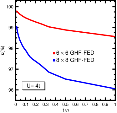
Figure 3: (Color online) The percentage of correlation energy $\kappa$ [Eq.(7)] obtained with the GHF-FED approximation is plotted as a function of the inverse of the number n of transformations for the half-filled 6 $\times$ 6 (red curve) and 8 $\times$ 8 (blue curve) lattices. Results are shown for U=4t.

The auxiliary-field QMC approximation is an important tool for studying correlated electronic systems. Stripes-Shiwei The relevance of symmetries within this framework has already been discussed in the literature. Shiwei-QMC-Symmetry In Table 1, we compare ground state energies per site provided by our GHF-FED scheme for the 4 $\times$ 4 lattice at different doping fractions $x$ and onsite interactions of U=4t, 8t, and 12t with those obtained within the constrained-path (CPQMC) and release-constraint (RCQMC) QMC approximations. Both the CPQMC and RCQMC calculations were based on multideterminantal trial wave functions with symmetries obtained in the spirit of a small complete active-space self-consistent field (CASSCF) calculation. Shiwei-QMC-Symmetry For each configuration, the corresponding set of symmetry quantum numbers $\Theta$ is also given in the table. It is satisfying to observe that for the considered number n of symmetry-projected configurations, the GHF-FED energies are slightly more accurate than the CPQMC ones and reach the accuracy of the RCQMC results. The comparison with ED calculations, in the last column of the table, indicates that for this small lattice both the GHF-FED and RCQMC energies can be considered exact Shiwei-QMC-Symmetry ; Dagotto-Moreo-1992 for practical purposes.

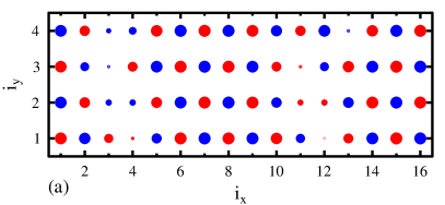
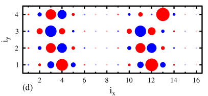
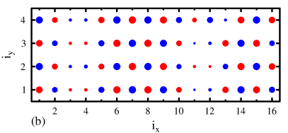
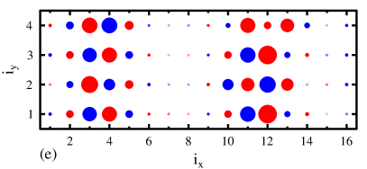
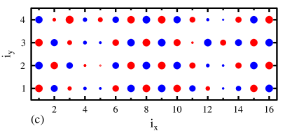
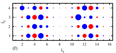
Figure 4: (Color online) The spin $\xi^{r}({\bf{i}})$ [Eq.(8)] and charge $\xi_{ch}^{r}({\bf{i}})$ [Eq.(9)] densities obtained with some typical intrinsic determinants resulting from the UHF-FED variational scheme are depicted in panels (a) to (c) and (d) to (f), respectively. Results are shown, for the 16 $\times$ 4 lattice with $N_{e}$=56 electrons at U=8t. The size of the circles is proportional to the value of the densities at a given lattice site ${\bf{i}}$. Blue (red) circles refer to spin up (down) in panels (a) to (c) and positve (negative) charge in panels (d) to (f). For details, see the main text.

We have recently explored the role of SR symmetry-projected trial states within the CPQMC framework. PaperwithShiwei It has been shown, through a hierarchy of calculations based on symmetry-projected trial states, that they increase the energy accuracy and decrease the statistical variance as more symmetries are broken and restored. The energies obtained within the CPQMC approach based on SR symmetry-projected UHF and GHF states (here, we use the acronyms SR-UHF-CPQMC and SR-GHF-CPQMC, ACRONY respectively) are compared in Table II with those obtained via MR UHF-FED and GHF-FED calculations in the case of a 4 $\times$ 4 lattice with 12 and 14 electrons at U=4t and 8t. One observes a good agreement between all these approximations that compare well with the ED results Shiwei-QMC-Symmetry ; PaperwithShiwei listed in the last column of the table. Note also that the energies in Tables I and II vastly improve those obtained in our previous study Rayner-2D-Hubbard-PRB-2012 of the 4 $\times$ 4 Hubbard model as a result of the (more correlated) MR character of the ansatz of Eq.(2) which also incorporates restoration of the space group symmetry.

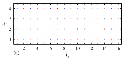
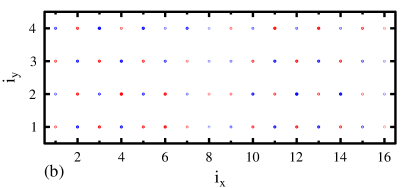
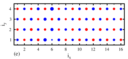
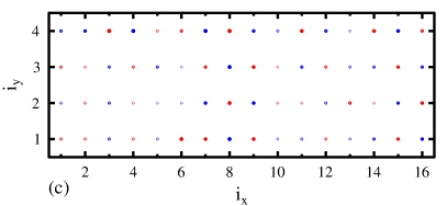
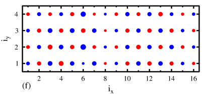
Figure 5: (Color online) The same as Fig. 4 but for U=2t.

The previous results illustrate that for half-filled and doped lattices up to 16 sites, the FED scheme provides essentially exact ground state energies. The question naturally arises as to whether reasonably correlated wave functions can also be obtained for larger 2D systems. The percentage of correlation energies

$$\kappa_{GHF-FED}=\frac{E_{RHF}-E_{GHF-FED}}{E_{RHF}-E_{EXACT}}\times 100\%$$ (7)

obtained with the GHF-FED approximation is plotted in Fig. 3 as a function of the inverse of the number n of transformations for the half-filled 6 $\times$ 6 (red curve) and 8 $\times$ 8 (blue curve) lattices at U=4t. The corresponding ground states are characterized by the ¹B₁ and ¹A₁ symmetries, respectively. In Eq.(7), $E_{RHF}$ is the energy of the standard restricted HF (RHF) solution, StuberPaldus ; HFclassification that preserves all the symmetries of the 2D Hubbard Hamiltonian. For the exact ground state energies of the 6 $\times$ 6 and 8 $\times$ 8 systems, we have used the estimates -30.89(1)t and -55.09(3)t, respectively. Shiwei-private-6by6 ; aux-QMC-Imada

The first noticeable feature from Fig. 3 is that even a SR calculation recovers a large portion of the correlation energy ($\kappa_{GHF-FED}$= 98.57 $\%$ and 96.05 $\%$ for the 6 $\times$ 6 and 8 $\times$ 8 lattices, respectively). These values already represent a vast improvement with respect to the standard UHF ones (79 $\%$ and 77 $\%$). The correlation energies increase smoothly with the number of symmetry-projected GHF basis states included in the FED expansion. It is also apparent from the figure that with increasing lattice size, we need to increase the number n of transformations to keep and/or improve the quality of our MR wave functions. For example, while n=10 transformations provide an essentially exact ground state for the half-filled 4 $\times$ 4 lattice (see, Table I), the corresponding energies (i.e., -30.8316t and -54.7157t) lead us to $\kappa_{GHF-FED}$=99.46 $\%$ and 97.90 $\%$ for the 6 $\times$ 6 and 8 $\times$ 8 ones. On the other hand, a further increase of the number of symmetry-projected GHF configurations up to n=120 and n=108 provides the ground state energies -30.8695t and -54.9242t ($\kappa_{GHF-FED}$= 99.81 $\%$ and 99.07 $\%$). Note that, in the case of the 6 $\times$ 6 lattice, our results also improve significantly the energy (i.e., -30.5766t) reported in our previous study. Rayner-2D-Hubbard-PRB-2012 A similar behavior is observed away from half-filling. For example, for a 6 $\times$ 6 lattice with N_e=24 electrons (¹B₁ symmetry) at U=4t we have obtained the energies per site of -1.17884t and -1.18445t with n=10 and n=180 symmetry-projected GHF configurations. The energies provided by the CPQMC and RCQMC approximations based on CASSCF multideterminantal trial wave functions with symmetries are -1.18625(3)t and -1.18525(4)t, respectively. Shiwei-QMC-Symmetry

The previous examples, and the results already obtained for 1D lattices, rayner-Hubbard-1D-FED2013 ; rayner-Hubbard-1D-FED2014 reveal the inner workings of the FED approach: it is a MR VAP strategy to build reasonably correlated ground states, with well defined symmetry quantum numbers $\Theta$, in low-dimensional electronic systems. In fact, it represents a constructive approximation in which, regardless of the dimensionality of the considered lattice, the quality of the ansatz Eq.(2), can be systematically improved by increasing the number of nonorthogonal symmetry-projected basis states through chains of VAP calculations. Note that the FED wave function is a discretized form of the exact coherent state representation of a fermion state Perlemov and therefore becomes exact in the limit n $\rightarrow$ $\infty$. In practical applications, however, one is always limited to a finite set of transformations whose precise number for obtaining a given accuracy is difficult to assert beforehand because the nature of the underlying quantum fluctuations varies for different doping fractions $x$ and onsite repulsions (see, below). In the examples discussed above, we have especially tailored the number of symmetry-projected basis states so as to compare well with state-of-the-art ground state energies available in the literature. However, the constructive nature of the FED ansatz also allows us to specifically tailor the number of symmetry-projected basis states to capture the main trends in the physical properties of interest (see, Sec. III.2).

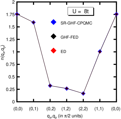
Figure 6: (Color online) The momentum distribution [Eq.(10)] provided by GHF-FED calculations (black diamonds) , based on n=40 transformations (see Table I), is compared with that obtained within the SR-GHF-CPQMC approach (blue diamonds) as well as with ED results (red diamonds). PaperwithShiwei Results are shown for a 4 $\times$ 4 lattice with N_e=14 electrons at U=8t. For details, see the main text.

We have considered two order parameters, i.e., the spin density (SD)

$$\xi^{r}({\bf{i}})=\langle{\cal{D}}^{r}|{\bf{S}}({\bf{i}})|{\cal{D}}^{r}\rangle\langle{\cal{D}}^{r}|{\bf{S}}({\bf{1}})|{\cal{D}}^{r}\rangle$$ (8)

and the charge density (CD)

$$\xi_{ch}^{r}({\bf{i}})=1-\sum_{\sigma}\langle{\cal{D}}^{r}|\hat{n}_{{\bf{i}}\sigma}|{\cal{D}}^{r}\rangle$$ (9)

associated with the symmetry-broken determinants $|{\cal{D}}^{r}\rangle$ resulting from UHF-FED calculations for a 16 $\times$ 4 lattice with N_e=56 electrons ($\delta=1-x$=1/8) at U=2t, 4t, 8t and 12t. We have restricted ourselves to n=40 symmetry-projected basis states which, as shown in the next Sec. III.2, is enough to capture the main features of the considered correlation functions. The ¹A₁ FED wave functions have the energies -82.1476t, -64.5369t, -44.4349t and -35.8096t, respectively. Obviously, these energies can be further improved by increasing the number of UHF transformations. Thus, for example, with n=200 we have obtained the value -65.1109t at U=4t. Note, that with n=40 ours are, from the energetical point of view, significantly better wave functions than the ones obtained in a routine SR symmetry-projected GHF calculation. Juillet Among all the UHF determinants $|{\cal{D}}^{r}\rangle$ used in the expansion Eq.(2) at U=8t and 2t, we have selected a typical subset to plot in Figs. 4 and 5 the corresponding SD [panels (a)-(c)] and CD [panels (d)-(f)] as functions of the lattice site ${\bf{i}}$.

It becomes apparent from Fig. 4 that the Slater determinants resulting from the UHF-FED VAP procedure contain structural defects in the SD at different lattice locations. In particular, they display vertical stripes separated by $\Delta i_{x}$ = 1/$\delta$ = 8 sites with deviations (fluctuations) from the pattern obtained with the UHF approximation. Xu-Chang-Walter-Shiwei-UHF-stripes One also observes that the charges delocalize within $\Delta i_{x}$ $\approx$ 1/2$\delta$ = 4 sites. Similar results are obtained for U=12t. From a theoretical point of view, stripes can be viewed as generic semiclassical instabilities in doped Mott-Hubbard insulators, Zaanen-Oles first pointed out by Tranquada et al. Tranquada and subsequently studied by several authors. Stripes-Shiwei ; White-stripes ; Hager-stripes The fluctuating stripes encode one possible kind of basic unit of quantum fluctuations in the MR UHF-FED wave functions. We stress that a doping x =7/8 is commensurate with the appearance of two stripes in the 16 $\times$ 4 lattice. Stripes-Shiwei The comparison with Fig. 5 reveals that even though defects are also present, the nature of the quantum fluctuations is completely different in the weak interaction regime with the charges spread all over the lattice. The same is also true for U=4t although in this case the charges start to display a tendency to localize around particular lattice sites. These results already suggest a transition to a stripe regime for increasing U values, as predicted within the auxiliary-field QMC framework. Stripes-Shiwei Furthermore, since the space group and spin projection operators can only translate by one site and rotate defects in the intrinsic states $|{\cal{D}}^{r}\rangle$ but do not destroy them, one may expect, as shown to be the case in Sec. III.2, that our MR symmetry-projected wave functions capture such a transition and reflect it in the corresponding correlation functions.

A rich variety of defects is also found in other lattices at different doping fractions $x$ and/or U values. We have also performed UHF-FED calculations for a 10 $\times$ 10 lattice with N_e = 92, 96 and 100 electrons at U=8t. We have restricted ourselves to a sample of n=70 symmetry-projected basis states, which is more than enough to obtain information about the basic units of quantum fluctuations in the intrinsic states $|{\cal{D}}^{r}\rangle$. The energies associated with the corresponding ¹A₁ and ¹B₁ states are -60.6629t, -55.2559t and -50.8999t, respectively, which already improve the available ResHF values. Tomita-2 For example, at half-filling, we have found (neutral) T-shaped defects similar to those predicted within the UHF-ResHF approximation. Tomita-2 Due to the presence of several close lying solutions, which are a consequence of the non linear character of the UHF-FED and/or GHF-FED ansätze, a more detailed analysis of the corresponding defects is left for future work. However we stress that similar to the 1D case, Tomita-1 ; rayner-Hubbard-1D-FED2013 ; rayner-Hubbard-1D-FED2014 both the FED and the ResHF VAP strategies provide intrinsic HF determinants whose defects encode information about the basic units of quantum fluctuations in the considered 2D systems.

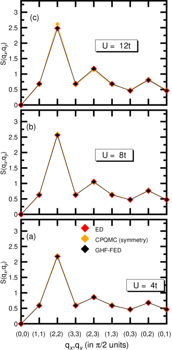
Figure 7: (Color online) Fourier transforms of the GHF-FED ground-state spin-spin correlation functions in real space [Eq.(11)] for a 4 $\times$ 4 lattice with N_e= 14 electrons (black diamonds) are compared with CPQMC results based on trial wave functions with symmetries (orange diamonds). ED values are depicted with red diamonds. Shiwei-QMC-Symmetry Results are shown for the onsite interactions 4t (a), 8t (b) and 12t (c). For more details, see the main text.

III.2 Momentum distributions and correlation functions

In this section, we turn our attention to both momentum distributions and correlation functions. It has been shown within the auxiliary-field QMC framework, PaperwithShiwei ; Shiwei-QMC-Symmetry that trial states with symmetries are important to account for SSCFs and momentum distributions. Therefore, it is interesting to study to which extent our MR wave functions, with well defined quantum numbers $\Theta$, can account for the main trends in those physical quantities. To this end, we first discuss our benchmark calculations for a 4 $\times$ 4 lattice. The momentum distribution reads

$$n^{\Theta}({\bf{q}})=\sum_{\sigma}\frac{\langle\phi_{K}^{\Theta}|{\hat{n}}_{{\bf{q}}\sigma}|\phi_{K}^{\Theta}\rangle}{\langle\phi_{K}^{\Theta}|\phi_{K}^{\Theta}\rangle}$$ (10)

where ${\hat{n}}_{{\bf{q}}\sigma}$ is the $\sigma$-occupation at wave vector ${\bf{q}}$.

In Fig. 6, we have plotted the ground state momentum distribution computed with the GHF-FED scheme (black diamonds) based on n=40 transformations (see Tables I and II), for a 4 $\times$ 4 lattice with N_e=14 electrons at U=8t. It is compared with the one obtained within the SR-GHF-CPQMC approach (blue diamonds), as well as with ED results (red diamonds). PaperwithShiwei We observe an excellent agreement between ours, the SR-GHF-CPQMC momentum distribution, and the one resulting from ED calculations.

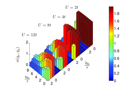
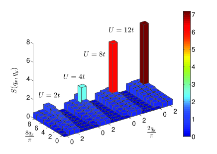
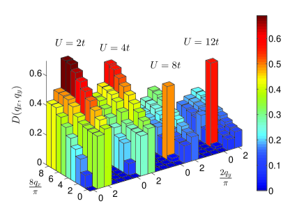
Figure 8: (Color online) Momentum distribution [Eq.(10)] provided by UHF-FED calculations, based on n=40 transformations, for the 16 $\times$ 4 lattice with N_e=56 electrons is shown in the top panel while the middle and bottom panels depict the Fourier transforms of the SSCFs [Eq.(11)] and CCCFs [Eq.(12)] in real space. Only the upper right quarter of the Brillouin zone is shown. Results are presented for U=2t, 4t, 8t, and 12t. For more details, see the main text.

For the same system, we have also computed the SSCFs $S_{m}^{\Theta}({\bf{i}})$ in real space

$$S_{m}^{\Theta}({\bf{i}})=\frac{4}{3}\frac{\langle\phi_{K}^{\Theta}|\hat{\bf{S}}({\bf{i}})\cdot\hat{\bf{S}}({\bf{1}})|\phi_{K}^{\Theta}\rangle}{\langle\phi_{K}^{\Theta}|\phi_{K}^{\Theta}\rangle}$$ (11)

where the subindex $m$ accounts for the irreducible representation of the space group used in the symmetry-projected calculations. rayner-Hubbard-1D-FED2013 ; rayner-Hubbard-1D-FED2014 The Fourier transforms of the GHF-FED SSCFs (black diamonds) are compared in Fig. 7 with CPQMC results based on CASSCF multideterminantal trial wave functions with symmetries (orange diamonds) and ED values (red diamonds). Shiwei-QMC-Symmetry Results are shown for the onsite interactions 4t (a), 8t (b) and 12t (c). Regardless of the considered U values, we observe that the use of states with well defined symmetry quantum numbers, both within the GHF-FED and CPQMC schemes, lead to SSCFs that agree well with the ED ones.

Calculations have also been performed for the half-filled 6 $\times$ 6 and 8 $\times$ 8 lattices. With only one symmetry-projected GHF configuration we have obtained the values $S(\pi,\pi)$ = 6.0283 and 9.6164, respectively, for the Fourier transform of the SSCF at the wave vector ${\bf{q}}=(\pi,\pi)$. On the other hand, the MR GHF-FED wave functions already discussed in Sec. III.1 (i.e., n=120 and 108) lead us to $S(\pi,\pi)$ = 5.8245 and 8.3173, which should be compared with the auxiliary-field QMC estimates of 5.82(3) and 8.2(2). aux-QMC-Imada Therefore, through the VAP constructive increase of its basis states, Eq.(2), the FED scheme improves not only the ground state energies of the considered lattices, as already discussed in Sec. III.1, but also captures the most relevant spin-spin correlations.

The momentum distributions and the Fourier transforms of the ground state SSCFs and CCCFs obtained with UHF-FED calculations (n=40) for a 16 $\times$ 4 lattice with N_e=56 electrons are shown in Fig. 8 for U=2t, 4t, 8t, and 12t. We have tested that the number of basis states is large enough to already capture the main features of the considered quantities and that the corresponding profiles, especially those for large U values, are not significantly modified by further increasing n. At U=2t, the momentum distribution [Eq.(10)] (top panel) resembles, to a large extent, the one corresponding to a noninteracting Fermi gas where the states below the Fermi surface are occupied. With increasing onsite repulsions the momentum distributions are smeared out.

The Fourier transforms of the SSCFs [Eq.(11)] (middle panel) exhibit a broad background for all the considered U values. For both U=2t and 4t, there exists a weak antiferromagnetic peak at wave vector ${\bf{q}}=(\pi,\pi)$ which already disappears at U=8t. On the other hand, at U=4t, a peak can already be seen at ${\bf{q}}=(7\pi/8,\pi)$ which becomes more prominent as the onsite interaction is increased, signaling the emergence of inconmesurate spin-spin correlations. Furthermore, we have studied the CCCFs given by

$$D_{m}^{\Theta}({\bf{i}})=\frac{\langle\phi_{K}^{\Theta}|\hat{n}_{\bf{i}}\hat{n}_{\bf{1}}|\phi_{K}^{\Theta}\rangle}{\langle\phi_{K}^{\Theta}|\phi_{K}^{\Theta}\rangle}$$ (12)

where $\hat{n}_{\bf{i}}=\sum_{\sigma}\hat{n}_{{\bf{i}}\sigma}$. The corresponding Fourier transforms are shown in the bottom panel of Fig. 8. In this case, the quantity N${}_{e}^{2}$/N${}_{sites}^{2}$ has been subtracted to take out the trivial peak at the origin ${\bf{q}}=(0,0)$. For both U=2t and 4t, they are broad with little features. However, already at U=8t a peak appears at wave vector ${\bf{q}}=(\pi/4,0)$ signaling the development of charge order. The previous results for SSCFs and CCCFs, are consistent with the crossover to a stripe regime already anticipated in Sec. III.1 in terms of the intrinsic determinants resulting from the UHF-FED VAP procedure. They agree well with the ones obtained within the CPQMC approach. Stripes-Shiwei

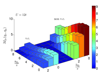
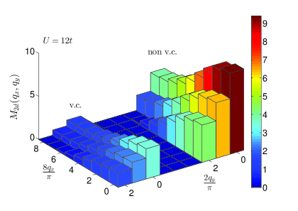
Figure 9: (Color online) Fourier transforms of the 2s (extended s-wave) and 2d (d${}_{x^{2}-y^{2}}$ wave) PCFs provided by UHF-FED calculations, based on n=40 transformations, for the 16 $\times$ 4 lattice with N_e=56 electrons are depicted, with (v.c) and without (non v.c) vertex corrections, in the top and bottom panels. Results are shown for U=12t. For more details, see the main text.

Finally, the PCFs are defined in real space as

$$M_{m}^{\Theta}({\bf{i}})=\frac{\langle\phi_{K}^{\Theta}|\hat{\Delta}_{\bf{1}}\hat{\Delta}_{\bf{i}}^{\dagger}|\phi_{K}^{\Theta}\rangle}{\langle\phi_{K}^{\Theta}|\phi_{K}^{\Theta}\rangle}$$ (13)

with

$$\hat{\Delta}_{\bf{i}}=\sum_{{\bf{R}}}f({\bf{R}})\Big{[}\hat{c}_{{\bf{i}}\uparrow}\hat{c}_{{\bf{i}}+{\bf{R}}\downarrow}-\hat{c}_{{\bf{i}}\downarrow}\hat{c}_{{\bf{i}}+{\bf{R}}\uparrow}\Big{]}$$ (14)

where $f({\bf{R}})$ is a form factor that depends on the pairing mode under consideration. aux-QMC-Imada We have paid attention to the 2s (extended s-wave) and 2d (d${}_{x^{2}-y^{2}}$) pairing modes defined by the following form factors

$$f_{2s}({\bf{R}})=\delta_{R_{y},0}\sum_{l=-1,1}\delta_{R_{x},l}+\delta_{R_{x},0}\sum_{l=-1,1}\delta_{R_{y},l}$$

$$f_{2d}({\bf{R}})=\delta_{R_{y},0}\sum_{l=-1,1}\delta_{R_{x},l}-\delta_{R_{x},0}\sum_{l=-1,1}\delta_{R_{y},l}$$ (15)

For each mode, we have considered PCFs with (v.c) and without (non v.c) vertex corrections. In the former case, we have replaced the two-electron density matrix $\rho({\bf{i}}_{1}\sigma_{1},{\bf{i}}_{2}\sigma_{2},{\bf{i}}_{3}\sigma_{3},{\bf{i}}_{4}\sigma_{4})=\langle\hat{c}_{{\bf{i}}_{1}\sigma_{1}}^{\dagger}\hat{c}_{{\bf{i}}_{2}\sigma_{2}}^{\dagger}\hat{c}_{{\bf{i}}_{3}\sigma_{3}}\hat{c}_{{\bf{i}}_{4}\sigma_{4}}\rangle$ by $\omega({\bf{i}}_{1}\sigma_{1},{\bf{i}}_{2}\sigma_{2},{\bf{i}}_{3}\sigma_{3},{\bf{i}}_{4}\sigma_{4})=\rho({\bf{i}}_{1}\sigma_{1},{\bf{i}}_{2}\sigma_{2},{\bf{i}}_{3}\sigma_{3},{\bf{i}}_{4}\sigma_{4})-\rho({\bf{i}}_{4}\sigma_{4},{\bf{i}}_{1}\sigma_{1})\rho({\bf{i}}_{3}\sigma_{3},{\bf{i}}_{2}\sigma_{2})+\rho({\bf{i}}_{3}\sigma_{3},{\bf{i}}_{1}\sigma_{1})\rho({\bf{i}}_{4}\sigma_{4},{\bf{i}}_{2}\sigma_{2})$. The quantities $\rho({\bf{i}}_{2}\sigma_{2},{\bf{i}}_{1}\sigma_{1})=\langle\hat{c}_{{\bf{i}}_{1}\sigma_{1}}^{\dagger}\hat{c}_{{\bf{i}}_{2}\sigma_{2}}\rangle$ are the one-electron density matrices rs and the mean values $\langle\dots\rangle$ are always taken with the FED state Eq.(2). With these definitions, a positive vertex-corrected PCF would imply that the effective electron-electron interaction enhances the considered pairing correlations with respect to a dressed single-particle picture. We have plotted the Fourier transforms of the 2s and 2d PCFs, with (v.c) and without (non v.c) vertex corrections, in the top and bottom panels of Fig. 9, respectively. Results are shown for U=12t, i.e., in the stripe regime. As expected, the vertex corrections do not change the profiles of the Fourier transforms which reflect the pronounced locality of the 2s and 2d pairing correlations in real space. In good agreement with previous studies, we observe weakly enhanced 2s and 2d pairing correlations. Moreo-Scalapino

IV Conclusions

In this work, we have applied the FED approach, previously considered only for 1D systems, to the repulsive 2D Hubbard model. Our main goal has been to test the method for both half-filled and doped lattices. We have compared our results for ground state and correlation energies with those obtained using other theoretical approximations. From the results reported in this work and those obtained in our previous studies, rayner-Hubbard-1D-FED2013 ; rayner-Hubbard-1D-FED2014 together with its parallelization properties, we conclude that regardless of the dimensionality and/or doping fraction of the considered lattices and through its constructive VAP building of a symmetry-projected basis, the FED scheme provides compact MR correlated wave functions, with well defined quantum numbers, whose quality can be systematically improved by increasing the number of basis states used in the expansion. In fact, the method could be seen as a symmetry-projected and variationally-truncated configuration-interaction (CI) approach. Carlo-review The key point is that the hierarchy of the truncation is transferred to a correlated basis of symmetry-projected multideterminantal (nonorthogonal) configurations. In this model, it is the Hamiltonian who determines via the Ritz variational principle [i.e., the Thouless theorem rs plus the resonon-like Eq.(6)], the relative weight of each of these nonorthogonal basis states for capturing the most relevant correlations in a given system via chains of calculations.

For different lattices sizes, doping fractions, and onsite interactions, we have found that the intrinsic determinants $|{\cal{D}}^{r}\rangle$ resulting from FED calculations display a wide variety of structural defects which encode information about the basic units of quantum fluctuations. For example, in the case of a 16 $\times$ 4 lattice with a commensurate doping fraction x=7/8, the varying structure of those defects and the associated charge densities, revealed the transition to a (fluctuating) stripe regime, which agrees well with previous results obtained with an auxiliary-field QMC approximation. Stripes-Shiwei Similar to the 1D case, rayner-Hubbard-1D-FED2013 ; rayner-Hubbard-1D-FED2014 the optimization of the intrinsic determinants in the presence of the projection operators induces such structural defects. It is precisely the action of the projection operators (rotations, translations by one lattice site, etc.) on these defects, as well as their interaction through the resonon-like Eq.(6), what brings about the substantial correlation energy obtained within the FED scheme compared to the usual mean-field HF calculations.

We have compared the FED momentum distributions and SSCFs with those obtained via the CPQMC approach based on trial wave functions with well defined symmetries PaperwithShiwei ; Shiwei-QMC-Symmetry for the case of a small 4 $\times$ 4 lattice with N_e=14 electrons. We conclude that the use of pure spin states leads to a good agreement between ours, the CPQMC, and ED values. We have then turned our attention to the computation of SSCFs and CCCFs for a 16 $\times$ 4 lattice with N_e=56 electrons. The corresponding results signal the emergence of incommensurate spin-spin correlations and the development of charge order for increasing onsite repulsions that is consistent with the transition to a stripe regime anticipated in terms of the structure of the intrinsic Slater states resulting from our variational strategy. Furthermore, in good agreement with previous studies, Moreo-Scalapino the (vertex-corrected) PCFs, computed with the MR FED wave functions, display a weak enhancement of the extended s-wave and d${}_{x^{2}-y^{2}}$ pairing modes.

The FED methodology has already been quite successful in microscopic nuclear structure theory, Carlo-review but it is still in its first steps in both quantum chemistry Carlos-Rayner-Gustavo-FED-molecules ; Laimis-paper and condensed matter physics. rayner-Hubbard-1D-FED2013 ; rayner-Hubbard-1D-FED2014 We believe that it is a good candidate for further multidisciplinary bridges between these research fields. In the realm of condensed matter physics, a long list of tasks awaits completion. Among others, a more detailed study of the structural defects resulting from our variational strategy is required including geometries other than square and rectangular ones, i.e., the honeycomb, triangular, and kagome lattices. Such studies could be useful to deepen the understanding of the basic units of quantum fluctuations in these lattices. Given the prominent role of defects, their careful classification within the FED approach could also be useful to further improve the quality of the starting intrinsic configurations used in our (highly nonlinear) optimizations.

Let us also stress that in this study, we have concentrated on the repulsive sector of the model. The FED approach can also be generalized to include, in addition to spin and space group, the restoration of the U(1) particle number symmetry on top of symmetry-broken Hartree-Fock-Bogoliobov states. Carlo-review This would allow us to also tackle the attractive sector of the Hubbard model.

- (1) E. Dagotto, Rev. Mod. Phys. 66, 763 (1994).
- (2) E. Dagotto, Rev. Mod. Phys. 85, 849 (2013).
- (3) F. H. L. Essler, H. Frahm, F. Göhmann, A. Klümper and V. E. Korepin, The One-Dimensional Hubbard Model (Cambridge University Press, Cambridge, 2005).
- (4) J. Voit, Phys. Rev. B 47, 6740 (1993).
- (5) M. Ogata and H. Shiba, Phys. Rev. B 41, 2326 (1990).
- (6) J. Hubbard, Proc. R. Soc. (London) A 276, 238 (1963).
- (7) F. Gebhard, The Mott Metal-Insulator Transition, Springer Tracts in Modern Physics Vol. 137 (Springer, Berlin, 1997).
- (8) B. J. Kim, H. Koh, E. Rotenberg, S. -J. Oh, H. Eisaki, N. Motoyama, S. Uchida, T. Tohoyama, S. Maekawa, Z. X. Shen and C. Kim, Nature 2, 397 (2006).
- (9) K. M. Shen, F. Ronning, D. H. Lu, W. S. Lee, N. J. C. Ingle, W. Meevasana, F. Baumberger, A. D. Damascelli, N. P. Armitage, L. L. Miller, Y. Kohsaka, M. Azuma, M. Takano, H. Takagi and Z. X. Shen, Phys. Rev. Lett. 93, 267002 (2004).
- (10) G. Fano, F. Ortolani and A. Parola, Phys. Rev. B 46, 1048 (1992).
- (11) H. De Raedt and W. von der Linden, The Monte Carlo Method in Condensed Matter Physics, edited by K. Binder (Springer-Verlag, Heidelberg, 1992).
- (12) Quantum Monte Carlo Methods in Physics and Chemistry edited by M. P. Nightingale and C. J. Umrigar, NATO Advanced Studies Institute, Series C: Mathematical and Physical Sciences (Kluwer, Dordrecht, 1999), Vol. 525.
- (13) H. Shi and S. Zhang, Phys. Rev. B 88, 125132 (2013).
- (14) E. Neuscamman, C. J. Umrigar and G. K.-L. Chan, Phys. Rev. B 85, 045103 (2012).
- (15) R. F. Bishop, P. H. Y. Li, D. J. J. Farnell, J. Richter and C. E. Campbell, Phys. Rev. B 85, 205122 (2012).
- (16) P. H. Y. Li, R. F. Bishop, D. J. J. Farnell, and C. E. Campbell, Phys. Rev. B 86, 144404 (2012).
- (17) J. R. Hammond and D. A. Mazzioti, Phys. Rev. A 73, 062505 (2006).
- (18) S. R. White, Phys. Rev. Lett. 69, 2863 (1992).
- (19) U. Schollwöck, Rev. Mod. Phys. 77, 259 (2005).
- (20) U. Schollwöck, Ann. Phys. 326, 96 (2010).
- (21) G. K.-L. Chan and S. Sharma, Ann. Rev. Phys. Chem. 62, 465 (2011).
- (22) L. Tagliacozzo, G. Evenbly and G. Vidal, Phys. Rev. B 80, 235127 (2009).
- (23) C. V. Kraus, N. Schuch, F. Verstraete and J. I. Cirac, Phys. Rev. A 81, 052338 (2010).
- (24) S. Singh and G. Vidal, Phys. Rev. B 88, 115147 (2013).
- (25) D. Zgid, E. Gull and G. K.-L. Chan, Phys. Rev. B 86, 165128 (2012).
- (26) T. Maier, M. Jarrell, T. Pruschke and M. H. Hettler, Rev. Mod. Phys. 77, 1027 (2005).
- (27) T. D. Stanescu, M. Civelli, K. Haule and G. Kotliar, Ann. Phys. 321, 1682 (2006).
- (28) A. Georges, G. Kotliar, W. Krauth and M. J. Rozenberg, Rev. Mod. Phys. 68, 13 (1996).
- (29) S. Moukouri and M. Jarrell, Phys. Rev. Lett. 87, 167010 (2001).
- (30) C. Huscroft, M. Jarrell, Th. Maier, S. Moukouri and A. N. Tahvildarzadeh, Phys. Rev. Lett. 86, 139 (2001).
- (31) K. Aryanpour, M. H. Hettler and M. Jarrell, Phys. Rev. B 67, 085101 (2003).
- (32) M. Potthoff, Eur. Phys. J. B 32, 429 (2003).
- (33) G. Knizia and G. K.-L. Chan, Phys. Rev. Lett. 109, 186404 (2012).
- (34) I. W. Bulik, G. E. Scuseria and J. Dukelsky, Phys. Rev. B 89, 035140 (2013).
- (35) I. W. Bulik, W. Chen and G. E. Scuseria, arXiv/physics.chem-ph/1406.2034 (2014).
- (36) Q. Chen, G. H. Booth, S. Sharma, G. Knizia, G. K.-L. Chan, Phys. Rev. B 89, 165134 (2014).
- (37) H. Bethe, Z. Phys. 71, 205 (1931).
- (38) E. H. Lieb and F. Y. Wu, Phys. Rev. Lett. 20, 1445 (1968).
- (39) N. Tomita, Phys. Rev. B 69, 045110 (2004).
- (40) N. Tomita and S. Watanabe, Phys. Rev. Lett. 103, 116401 (2009).
- (41) N. Tomita, Phys. Rev. B 79, 075113 (2009).
- (42) F. Satoh, M. Ozaki, T. Maruyama and N. Tomita, Phys. Rev. B 84, 245101 (2011).
- (43) K.W. Schmid, T. Dahm, J. Margueron and H. Müther, Phys. Rev. B 72, 085116 (2005).
- (44) R. Rodríguez-Guzmán, K.W. Schmid, C. A. Jiménez-Hoyos and G. E. Scuseria, Phys. Rev. B 85, 245130 (2012).
- (45) C. A. Jiménez-Hoyos, R. Rodríguez-Guzmán and G. E. Scuseria, Phys. Rev. A 86, 052102 (2012).
- (46) R. Rodríguez-Guzmán, C. A. Jiménez-Hoyos, R. Schutski and G. E. Scuseria, Phys. Rev. B 87, 235129 (2013).
- (47) R. Rodríguez-Guzmán, C. A. Jiménez-Hoyos and G. E. Scuseria, Phys. Rev. B 89, 195109 (2014).
- (48) C. A. Jiménez-Hoyos, R. Rodríguez-Guzmán and G. E. Scuseria, J. Chem. Phys. 139, 224110 (2013).
- (49) C. A. Jiménez-Hoyos, R. Rodríguez-Guzmán and G. E. Scuseria, J. Chem. Phys. 139, 204102 (2013).
- (50) L. Bytautas, Carlos A. Jiménez-Hoyos, R. Rodríguez-Guzmán and Gustavo E. Scuseria, Mol. Phys. 112, 1938 (2014).
- (51) G. E. Scuseria, C. A. Jiménez-Hoyos, T. M. Henderson, K. Samanta and J. K. Ellis, J. Chem. Phys. 135, 124108 (2011)
- (52) C. A. Jiménez-Hoyos, T. M. Henderson, T. Tsuchimochi and G. E. Scuseria, J. Chem. Phys. 136, 164109 (2012)
- (53) K. Samanta, C. A. Jiménez-Hoyos and G. E. Scuseria, J. Chem. Theory Comput. 8, 4944 (2012).
- (54) O. Juillet and R. Frésard, Phys. Rev. B 87, 115136 (2013).
- (55) P. Ring and P. Schuck, The Nuclear Many-Body Problem (Springer, Berlin, 1980).
- (56) K. W. Schmid, Prog. Part. Nucl. Phys. 52, 565 (2004).
- (57) K. W. Schmid, F. Grümmer and A. Faessler, Phys. Rev. C 29, 291 (1984).
- (58) R. Rodríguez-Guzmán and K. W. Schmid, Eur. Phys. J. A 19, 45 (2004).
- (59) R. Rodríguez-Guzmán and K. W. Schmid, Eur. Phys. J. A 19, 61 (2004).
- (60) R. Rodríguez-Guzmán, J. L. Egido and L. M. Robledo, Nucl. Phys. A 709, 201 (2002)
- (61) R. Rodríguez-Guzmán, L. M. Robledo and P. Sarriguren, Phys. Rev. C 86, 034336 (2012).
- (62) H. Fukutome, Prog. Theor. Phys. 80, 417 (1988); 81, 342 (1989).
- (63) S. Yamamoto, A. Takahashi and H. Fukutome, J. Phys. Soc. Jpn. 60, 3433 (1991).
- (64) S. Yamamoto and H. Fukutome, J. Phys. Soc. Jpn. 61, 3209 (1992).
- (65) A. Ikawa, S. Yamamoto, and H. Fukutome, J. Phys. Soc. Jpn. 62, 1653 (1993).
- (66) J. G. Bednorz and K. A. Müller, Z. Phys. B 64, 189 (1986).
- (67) P. W. Anderson, Science 235, 1196 (1987).
- (68) Theoretical Methods for Strongly Correlated Systems, edited by A. Avella and F. Mancini (Springer Verlag, Berlin, 2011).
- (69) J. E. Hirsch, Phys. Rev. B 31, 4403 (1985).
- (70) J. E. Hirsch and S. Tang, Phys. Rev. Lett. 62, 591 (1989).
- (71) S. R. White, D. J. Scalapino, R. L. Sugar, E. Y. Loh, J. E. Gubernatis and R. T. Scalettar, Phys. Rev. B 40, 506 (1989).
- (72) N. Furukawa and M. Imada, J. Phys. Soc. Jpn. 61, 3331 (1992).
- (73) R. Jördens, N. Strohmaier, K. Günter, H. Moritz and T. Esslinger, Nature 455, 204 (2008); U. Schneider, L. Hackermüller, S. Will, Th. Best, I. Bloch, T. A. Costi, R. W. Helmes, D. Rasch and A. Rosch, Science 322, 1520 (2008); I. Bloch, J. Dalibard and W. Zwerger, Rev. Mod. Phys. 80, 885 (2008).
- (74) A. H. Castro Neto, F. Guinea, N. M. R. Peres, K., S. Novosolev and A. K. Geim, Rev. Mod. Phys. 81, 109 (2009).
- (75) P. Dai, J. Hu and E. Dagotto, Nature 8, 709 (2012).
- (76) Y. Kamihara, T. Watanabe, M. Hirano and H. Hosono, J. Am. Chem. Soc. 130, 3296 (2008).
- (77) G. R. Stewart, Rev. Mod. Phys. 83, 1539 (2011).
- (78) E. Dagotto, Science 309, 257 (2005).
- (79) H. Ohta, S. Kim, Y. Mune, T. Mizoguchi, K. Nomura, S. Ohta, T. Nomura, Y. Nakanishi, M. Hirano, H. Hosono and K. Koumoto, Nature Mat. 6. 129 (2007).
- (80) S. Yan, D. A. Huse and S. R. White, Science 332, 1173 (2011).
- (81) Y. Iqbal, D. Poilblanc and F. Becca, Phys. Rev. B 89, 020407(R) (2014).
- (82) W. -J. Hu, F. Becca, A. Parola and S. Sorella, Phys. Rev. B 88, 060402(R) (2013).
- (83) J.-P. Blaizot and G. Ripka, Quantum Theory of Finite Fermi Systems (The MIT Press, Cambridge, MA, 1985).
- (84) J. L. Stuber and J.Paldus, Symmetry Breaking in the Independent Particle Model. Fundamental World of Quantum Chemistry: A Tribute Volume to the Memory of Per-Olov Löwdin; Edited by E. J. Brandas and E. S Kryachko (Kluwer, Dordrecht, 2003).
- (85) H. Fukutome, Int. J. Quantum Chem., 20, 955 (1981)
- (86) H. Shi, C. A. Jiménez-Hoyos, R. Rodríguez-Guzmán, G. E. Scuseria and S. Zhang, Phys. Rev. B 89, 125129 (2014).
- (87) K. W. Schmid, M. Kyotoku, F. Grümmer and A. Faessler, Ann. Phys. (NY) 190, 182 (1989).
- (88) S. Nishiyama, Prog. Theor. Phys. 69, 100 (1983).
- (89) A. Moreo and E. Dagotto, Phys. Rev. B 42, 4786 (1990).
- (90) R. M. Fye, M. J. Martins, D. J. Scalapino, J. Wagner and W. Hanke, Phys. Rev. B 45, 7311 (1992).
- (91) E. Jeckelmann, F. Gebhard and F. H. Essler, Phys. Rev. Lett. 85, 3910 (2000).
- (92) R. Rodríguez-Guzmán, C. A. Jiménez-Hoyos and G. E. Scuseria, in preparation.
- (93) A. R. Edmonds, Angular Momentum in Quantum Mechanics, Princeton University Press, Princeton (1957).
- (94) N.W. Ashcroft and N.D. Mermin, Solid State Physics, Saunders College, 1976.
- (95) M.C. Gutzwiller, Phys. Rev. Lett. 10, 159 (1963).
- (96) R. Rodríguez-Guzmán and L. M. Robledo, Phys. Rev. C 89, 054310 (2014).
- (97) D.C. Liu and J. Nocedal, Math. Program. B 45, 503 (1989).
- (98) C. -C. Chang and S. Zhang, Phys. Rev. Lett. 104, 116402 (2010).
- (99) E. Dagotto, A. Moreo, F. Ortolani, D. Poilblanc and J. Riera, Phys. Rev. C 45, 10741 (1992).
- (100) In our previous work PaperwithShiwei we have used the acronyms SG,S-UHF and SG,S-GHF, respectively.
- (101) S. Zhang (private communication).
- (102) T. Aimi and M. Imada, J. Phys. Soc. Jpn 76, 084709 (2007).
- (103) A.M. Perlemov, Sov. Phys. Usp. 20, 703 (1977).
- (104) J. Xu, C. Chia-Chen, E. Walter and S. Zhang, J. Phys. : Condens. Matter 23, 505601 (2011).
- (105) J. Zaanen and A. M. Olés, Ann. Phys. 5, 224 (1996).
- (106) J. M. Tranquada, B. J. Sternlieb, J. D. Axe, Y. Nakamura and S. Uchida, Nature 375, 561 (1995).
- (107) S. R. White and D. J. Scalapino, Phys. Rev. Lett. 91, 136403 (2003).
- (108) G. Hager, C. Wellein, E. Jeckelmann and H. Fehske, Phys. Rev. B 71, 075108 (2005).
- (109) A. Moreo and D. J. Scalapino, Phys. Rev. B 43, 8211 (1991).