Improved version of the PHOBOS Glauber Monte Carlo

Abstract

“Glauber” models are used to calculate geometric quantities in the initial state of heavy ion collisions, such as impact parameter, number of participating nucleons and initial eccentricity. Experimental heavy-ion collaborations, in particular at RHIC and LHC, use Glauber Model calculations for various geometric observables for determination of the collision centrality. In this document, we describe the assumptions inherent to the approach, and provide an updated implementation (v2) of the Monte Carlo based Glauber Model calculation, which originally was used by the PHOBOS collaboration. The main improvements w.r.t. the earlier version (v1) Alver:2008aq are the inclusion of Tritium, Helium-3, and Uranium, as well as the treatment of deformed nuclei and Glauber-Gribov fluctuations of the proton in p+A collisions. A users’ guide (updated to reflect changes in v2) is provided for running various calculations.

Revisions && changes of the arXiv document and code:
v1, 11 Aug 2014: initial document, code v2.0
v2, 20 Dec 2014: updated Table 1 with “p” and “PbHN”, code v2.1 (fixes bug for Hulthen)
v3, 01 Sep 2016: published version, fixed Eq. 3, code v2.3 (added $b_{\rm NN}$, and various proton profiles
v3, 01 Sep 2016: from Pythia, changes in calculation of $\varepsilon_{n}$)
v4, 07 Jun 2017: updated Table 1 with “Xe” and corrected typo in proton radius, code v2.4
v4, 07 Jun 2017: (fixed drawing function)
v5, 16 Oct 2017: updated Table 1 with “Pb*”
v6, 13 Nov 2017: updated Table 1 with “Xes”
v7, 01 Mar 2018: split previous Table 1 into two tables: Table 1 for spherical and Table 2 for
v4, 01 Mar 2018: deformed nuclei parameters, added “Xe2” and “Xe2a” to include deformation of
v7, 01 Mar 2018: Xenon, code v2.5 (included core/corona calculation, see “Npart0”)
v8, 30 Apr 2018: fixed typo in $Y_{20}$, fixed $\beta_{4}$ in “Si2”, added “Al”, describes new function
v8, 25 Apr 2018: runAndCalcDens, code v2.6 (includes fixes and “runAndCalcDens”)
v9, 14 Jan 2019: added Helium-4, Carbon and Oxygen from wavefunctions, unified deuteron
v9, 14 Jan 2019: treatment, added and new function runAndOutputLemonTree, updated Table 1,
v9, 14 Jan 2019: latest code v2.7 (includes new elements and “runAndOutputLemonTree”)

I Introduction

In heavy-ion collisions, initial geometric quantities such as impact parameter and shape of the collision region cannot be directly determined experimentally. However, it is possible to relate the number of observed particles and number of spectator neutrons to the centrality of the collision. Using the percentile centrality of a collision, the initial geometric configuration can be estimated with models assuming the configuration nuclei from nucleons and the collision process of two nuclei.

These models fall in two main classes. (For a review, see LABEL:glaubreview). In the so called “optical” Glauber calculations, a smooth matter density is assumed, typically described by a Fermi distribution in the radial direction and uniform over solid angle. In the Monte Carlo (MC) based models, individual nucleons are stochastically distributed event-by-event and collision properties are calculated by averaging over multiple events. As discussed in LABEL:glaubreview and LABEL:eccentricity, the two type of models lead to mostly similar results for simple quantities such as the number of participating nucleons ($N_{\rm part}$) and impact parameters ($b$), but give different results in quantities where event-by-event fluctuations are significant, such as participant frame eccentricity ($\epsilon_{\rm part}$).

In this paper, we discuss several improvements of the Monte Carlo Glauber calculation originally implemented by the PHOBOS collaboration Alver:2008aq . The main improvements w.r.t. the earlier version (v1) are the inclusion of Tritium, Helium-3, and Uranium, as well as the treatment of deformed nuclei and Glauber-Gribov fluctuations of the proton in p+A collisions. Another widely used implementation of a MC Glauber calculation can be found in LABEL:Rybczynski:2013yba. In section II, the MC approach is outlined and the assumptions that go into the calculation are introduced. In section III, we discuss the implementation and the tutorial functions provided. Section IV summarizes the paper. The latest version 2 code described in this document is v2.7. For further improvements, mainly focusing on nuclear collisions involving Pb at high collision energies, see LABEL:Loizides:2017ack.

II The model

The MC Glauber model calculation is performed in two steps. First, the nucleon positions in each nucleus are stochastically determined. Then, the two nuclei are “collided”, assuming the nucleons travel in a straight line along the beam axis (eikonal approximation) such that nucleons are tagged as wounded (participating) or spectator.

II.1 Makeup of nuclei

The position of each nucleon in the nucleus is determined according to a probability density function. In a quantum mechanical picture, the probability density function can be thought of as the single-particle probability density and the position as the result of a position measurement. In the context of the MC Glauber model, one commonly requires a minimum inter-nucleon separation ($d_{\rm min}$) between the centers of the nucleons for the determination of the nucleon positions inside a given nucleus.

The probability distribution for spherical nuclei is taken to be uniform in azimuthal and polar angles. The radial probability function is modeled from nuclear charge densities extracted in low-energy electron scattering experiments atomicdata . The nuclear charge density is usually parameterized by a Fermi distribution with three parameters

$$\rho(r)=\rho_{0}\frac{1+w(r/R)^{2}}{1+\exp(\frac{r-R}{a})}\,,$$ (1)

where $\rho_{0}$ is the nucleon density, $R$ is the nuclear radius, $a$ is the skin depth and $w$ corresponds to deviations from a spherical shape. The overall normalization ($\rho_{0}$) is not relevant for this calculation. Values of the other parameters used for different nuclei are listed in Table 1.

Exceptions from Eq. 1 are the Deuteron (²H), Tritium (H3, ³H), Helium-3 (He3, ³He), Helium-4 (He4, ⁴He), Carbon (C), Oxygen (O) and Sulfur (³²S) nuclei. For Sulfur, a three parameter Gaussian form is used

$$\rho(r)=\rho_{0}\frac{1+w(r/R)^{2}}{1+\exp(\frac{r^{2}-R^{2}}{a^{2}})}\,.$$ (2)

The values of $R$, $a$ and $w$ for Sulfur are also given in Table 1. For Deuteron, three options are supported with the $3^{\text{rd}}$ option being the one used in PHOBOS analyses:

1. The three parameter Fermi form with the values given in Table 1.

2. The Hulthén form

   $$\rho(r^{\prime})=\rho_{0}\left(\frac{e^{-ar^{\prime}}-e^{-br^{\prime}}}{r^{\prime}}\right)^{2},$$ (3)

   where $a=0.228$ fm^-1 and $b=1.177$ fm^-1, and $r^{\prime}$ denotes the distance between the proton and neutron, i.e. $r=r^{\prime}/2$ Hulthen ; deuteronpars ; Adler:2006xd .

3. The proton is taken from the Hulthén form given above with the neutron placed opposite to it.

For ³H and ³He, the configurations were computed (and stored in a database) from Green’s function MC calculations using the AV18 + UIX model interactions, which correctly sample the position of the three nucleons, including correlations, as in LABEL:Nagle:2013lja. Similarly, results of wavefunction-based calculations described in LABEL:Lim:2018huo were made available for He-4, Carbon and Oxygen. Finally, note that we also provide the rescaled values for the radius and skin depth of Cu (“CuHN”), Au (“AuHN”) and Pb (“PbHN”) to take into account the finite nucleon profile as derived in Hirano:2009ah and Shou:2014eya . For deformed nuclei we use

$$\rho(x,y,z)=\rho_{0}\frac{1}{1+\exp\frac{\left(r-R(1+\beta_{2}Y_{20}+\beta_{4}Y_{40})\right)}{a}}\,,$$ (4)

where $Y_{20}=\sqrt{\frac{5}{16\pi}}(3{\rm cos}^{2}(\theta)-1)$, $Y_{40}=\frac{3}{16\sqrt{\pi}}(35{\rm cos}^{4}(\theta)-30{\rm cos}^{2}(\theta)+3)$ with the deformation parameters $\beta_{2}$ and $\beta_{4}$ taken from Ref. atomicdata2 . The values used for different nuclei (Si, Cu, Au and U) are listed in Table 2.

Name	R [fm]	a [fm]	w
p	0.234
d	0.010	0.5882	-0.0000
H3
He3c
He4c
Cc
16Oc
16Opar	2.608	0.5130	-0.5100
16Oho	1.833	1.5440	-0.0000
28Si	3.340	0.5800	-0.2330
32S	2.540	2.1910	-0.1600
40Ar	3.530	0.5420	-0.0000
40Ca	3.766	0.5860	-0.1610
58Ni	4.309	0.5170	-0.1308
63Cu	4.200	0.5960	-0.0000
63CuHN	4.280	0.5000	-0.0000
129Xe	5.360	0.5900	-0.0000
129Xes	5.420	0.5700	-0.0000
186W	6.580	0.4800	-0.0000
197Au	6.380	0.5350	-0.0000
197AuHN	6.420	0.4400	-0.0000
207Pb	6.620	0.5460	-0.0000
207PbHN	6.650	0.4600	-0.0000
208Pb*	6.624	0.5490	-0.0000

Table 1: Nuclear charge density parameters for different nuclei taken from LABEL:atomicdata for equations 1, 2 and 3. All implemented configurations can be found in the code in the TGlauNucleus::Lookup function.

Name	R [fm]	a [fm]	w	$\beta_{2}$	$\beta_{4}$
27Al	3.340	0.5800	0	-0.448	-0.239
28Si2	3.340	0.5800	-0.233	-0.478	-0.250
63Cu2	4.200	0.5960	0	-0.162	-0.006
129Xe2	5.360	0.5900	0	0.161	-0.003
129Xe2a	5.360	0.5900	0	0.18	-0
197Au2	6.380	0.5350	0	-0.131	-0.031
238U2	6.670	0.4400	0	-0.280	-0.093
238U	6.670	0.4400	0	-0.280	-0.093

Table 2: Nuclear charge density parameters for deformed nuclei taken from LABEL:atomicdata2. The “2” for Si2, Cu2, Au2 and U2 refers to the use of Eq. 4. All implemented configurations can be found in the code in the TGlauNucleus::Lookup function.

Figure 1: Typical events for Cu+Cu (top panel), Au+Au (middle panel), and Pb+Pb (lower panel) collisions, the first two performed at RHIC energies and the latter at the LHC. Wounded nucleons (participants) are indicated as solid circles, while spectators are dotted circles.

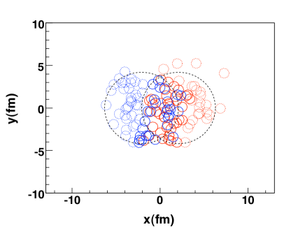
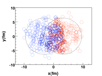
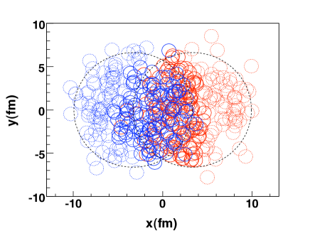
II.2 Collision Process

The impact parameter of the collision is chosen randomly from a distribution ${\rm d}N/{\rm d}b\propto b$ up to some large maximum $b_{\rm max}$ with $b_{\rm max}\simeq 20\,$fm$>2R_{A}$. The centers of the nuclei are calculated and shifted to $(-b/2,0,0)$ and $(b/2,0,0)$. The reaction plane, defined by the impact parameter and the beam direction, is given by the $x$- and $z$-axes, while the transverse plane is given by the $x$- and $y$-axes. It is assumed that the nucleons move along a straight trajectory along the beam axis. The longitudinal coordinate does not play a role in the calculation.

The inelastic nucleon-nucleon cross section ($\sigma_{\scriptscriptstyle{{\rm NN}}}$), which is only a function of the collision energy, is extracted from p+p collisions. A value of $\sigma_{\scriptscriptstyle{{\rm NN}}}=42$ mb is used at top RHIC energy of $\sqrt{s_{\scriptscriptstyle{{\rm NN}}}}=200$ GeV, while at the LHC $\sigma_{\scriptscriptstyle{{\rm NN}}}=64$ mb for $\sqrt{s_{\scriptscriptstyle{{\rm NN}}}}=2.76$ TeV and $\sigma_{\scriptscriptstyle{{\rm NN}}}=70$ mb for $\sqrt{s_{\scriptscriptstyle{{\rm NN}}}}=5.02$ TeV are used glauberlhc . When estimating the systematic uncertainties on calculated quantities like $N_{\rm part}$ one varies the $\sigma_{\scriptscriptstyle{{\rm NN}}}$ (along with the other parameters) by typically $\pm$3 mb and $\pm$5 mb at RHIC and LHC, respectively.

The “ball diameter” defined as

$$D=\sqrt{\sigma_{\scriptscriptstyle{{\rm NN}}}/\pi}$$ (5)

parameterizes the interaction strength of two nucleons: Two nucleons from different nuclei are assumed to collide if their relative transverse distance is less than the ball diameter. If no such nucleon–nucleon collision is registered for any pair of nucleons, then no nucleus–nucleus collision occurred. Counters for determination of the total (geometric) cross section are updated accordingly.

III Users’ guide

The MC Glauber code works within the ROOT framework (ROOT 4.00/08 or higher root ). The code is contained in the macro runglauber_vX.Y.C glaucode . The version described here is v2.7. Three classes, TGlauNucleon, TGlauNucleus and TGlauberMC and three functions (macros) runAndSaveNtuple(), runAndSaveNucleons(), and runAndSmearNtuple() are defined in the provided macro. Note that for generating events with ³H or ³He you will need the text files called “h3_plaintext.dat” or “he3_plaintext.dat” in the current path. While the functionality is essentially complete for known applications of the Glauber approach, users are encouraged to write their own functions to access results of the Glauber simulation or to modify the code.

The main classes are the following:

• TGlauNucleon is used to store information about a single nucleon. The stored quantities are the position of the nucleon, the number of binary collisions that the nucleon has had and which nucleus the nucleon is in, “A” or “B”. For every simulated event, the user can obtain an array containing all nucleons (via TGlauberMC::GetNucleons()).

• TGlauNucleus is used to generate and store information about a single nucleus. The user is not expected to interact with this class.

• TGlauberMC is the main steering class used to generate events and calculate event-by-event quantities such as the number of participating nucleons.

The steering class TGlauberMC has one constructor

TGlauberMC::TGlauberMC(Text_t* NA,
                       Text_t* NB,
                       Double_t xsect,
                       Double_t xsectsigma)

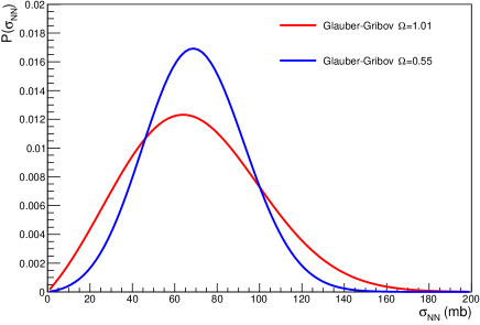
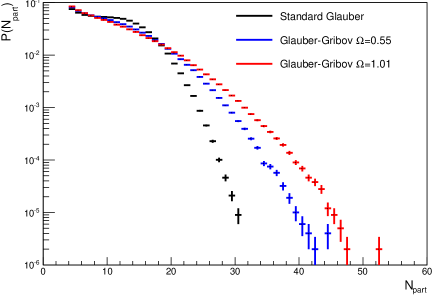
where NA and NB are the names of the colliding nuclei and xsect and xsectsigma are the nucleon-nucleon cross section mean and width given in mb. The defined nuclei names are given in Tables 1 and 2. For Deuteron, the names “d”, “dhh” and “dh” correspond to the three options described in section II.1 respectively. Units are generally given in fm for distances, while in mb for cross sections. If a finite value ($>0$) for the width of the cross section is given, the calculation will use the Glauber-Gribov model for fluctuations of the proton. This option was originally only implemented for p+A collisions, but can also be enabled for A+A collisions using the member function “SetCalcAAGG”. In this case, following Alvioli:2013vk as described in Aad:2015zza $\sigma_{\scriptscriptstyle{{\rm NN}}}$ will be distributed according to $1/\lambda\,P(\sigma/\lambda)$ with

$$P=\rho\frac{\sigma}{\sigma+\sigma_{0}}\exp^{-\left(\frac{\sigma-\sigma_{0}}{\sigma_{0}\,\Omega}\right)^{2}}\,$$ (6)

where $\sigma_{0}$ denotes the mean $\sigma_{\scriptscriptstyle{{\rm NN}}}$ and $\Omega$ the width. The normalization $\rho$ and the rescaling parameter $\lambda=\sigma_{0}/\left<\sigma\right>$ are computed from the provided input (mean $\sigma_{\scriptscriptstyle{{\rm NN}}}$ and $\Omega$) making use of $\int\sigma P{\rm d}\sigma/\int P{\rm d}\sigma=\sigma_{0}$ with $P=\rho\sigma_{0}\frac{x}{x+1}\exp^{-\left(\frac{x-1}{\Omega}\right)^{2}}$ for $x=\sigma/\sigma_{0}$. Example distributions for p+Pb collisions at the LHC are given in Fig. 2.

Figure 2: Distribution of $\sigma_{\scriptscriptstyle{{\rm NN}}}$ for mean $70$ mb with $\Omega=0.55$ and $1.01$ (top panel) and resulting $N_{\rm part}$ distributions calculated with the Glauber-Gribov extension of the MC Glauber model compared to the standard MC Glauber for p+Pb collisions at the LHC (bottom panel).

III.1 Running the Code

To generate Au+Au collisions at $\sqrt{s_{\scriptscriptstyle{{\rm NN}}}}=200$ GeV ($\sigma_{\scriptscriptstyle{{\rm NN}}}=42$ mb) one has to construct a TGlauberMC object by issuing at the “root” prompt the commands:

root [0] gSystem->Load("libMathMore")
root [1] .L runglauber_X.Y.C+
root [2] TGlauberMC glauber("Au","Au",42);

where the first ROOT command loads the needed library libMathMore, the second compiles, links and loads the compiled macro (where you have to replace X.Y with the current version number of the code, for example v2.7) including the Glauber code as explained in chapter 2 of the ROOT users’ guide, while the third commands sets up the Glauber simulation for Au+Au collisions at $\sqrt{s_{\scriptscriptstyle{{\rm NN}}}}=200$ GeV.

Events can be generated interactively using the two functions

• TGlauberMC::NextEvent(Double_t bgen), which is used to run an event at a specified impact parameter, or over a range of impact parameters (if bgen=-1, the default value) as described in section II.2).

• TGlauberMC::Run(Int_t nevents) which is used to run a large event sample by invoking NextEvent many times.

Other important public member functions are:

• TGlauberMC::SetMinDistance(Double_t d), which is used to set minimum nucleon separation within a nucleus, $d_{\rm min}$ (default is $0.4$ fm)

• TGlauberMC::SetBmin(Double_t bmin) and TGlauberMC::SetBmax(Double_t bmax), which can be used to set the range of impact parameter values generated in Run().

• TGlauberMC::GetTotXSect() which returns the total nucleus-nucleus cross section, calculated when the function Run() is called.

• TGlauberMC::Draw() which draws the current event in the current pad.

III.2 Provided functions

Four functions (macros) are provided to demonstrate how to run the model:

III.2.1 runAndSaveNtuple

The macro runAndSaveNtuple() generates a number of Monte Carlo events and saves some event-by-event quantities. It takes as parameters, the number of events to be generated, the collision system, the nucleon-nucleon cross section, its width to simulate Glauber-Gribov fluctuations (for p+A), the minimum separation distance and the output file name. It creates and stores an ntuple in the output file with the following event-by-event quantities:

• Npart: Number of participating nucleons.

• Npart0: Number of singly-wounded participating nucleons.

• Ncoll: Number of binary collisions.

• B: Generated impact parameter.

• BNN: Mean nucleon–nucleon impact parameter

• MeanX: Mean of $x$ for wounded nucleons, $\{x\}$.

• MeanY: Mean of $y$ for wounded nucleons, $\{y\}$.

• MeanX2: Mean of $x^{2}$ for wounded nucleons, $\{x^{2}\}$.

• MeanY2: Mean of $y^{2}$ for wounded nucleons, $\{y^{2}\}$.

• MeanXY: Mean of $xy$ for wounded nucleons, $\{xy\}$.

• VarX: Variance of $x$ for wounded nucleons, $\sigma_{x}^{2}$.

• VarY: Variance of $y$ for wounded nucleons, $\sigma_{y}^{2}$.

• VarXY: Covariance of $x$ and $y$ for wounded nucleons, $\sigma_{xy}\equiv\{xy\}-\{x\}\{y\}$.

• MeanXSystem: Mean of $x$ for all nucleons.

• MeanYSystem: Mean of $y$ for all nucleons.

• MeanXA: Mean of $x$ for nucleons in nucleus A.

• MeanYA: Mean of $y$ for nucleons in nucleus A.

• MeanXB: Mean of $x$ for nucleons in nucleus B.

• MeanYB: Mean of $y$ for nucleons in nucleus B.

• NpartA: $N_{\rm part}$ from nucleus A.

• NpartB: $N_{\rm part}$ from nucleus B.

• PhiA: Azimuthal angle for nucleus A.

• ThetaA: Polar angle for nucleus A.

• PhiB: Azimuthal angle for nucleus B.

• ThetaB: Polar angle for nucleus B.

• PsiN: Event plane angle of Nth harmonic.

• EccN: Participant eccentricity for Nth harmonic.

It is important to note that for each of these event-by-event quantities a “getter” function is implemented providing the users the option to write their own event loop (using TGlauberMC::NextEvent()).

III.2.2 runAndSaveNucleons

The macro runAndSaveNucleons() generates a number of Monte Carlo events and saves an array of TGlauNucleon objects for each event. It is also possible to use this function to print out the values stored in the nucleons by setting the verbosity parameter. The function takes as parameters the number of events to be generated, the collision system, the nucleon-nucleon cross section, the minimum separation distance, the verbosity flag, minimum and maximum impact parameter and the output file name.

III.2.3 runAndSmearNtuple

The macro runAndSmearNtuple() generates a number of Monte Carlo events and saves a reduced set of event-by-event quantities, where the position of the nucleon is smeared similar to what is done in Ref. Nagle:2013lja . It takes the same arguments as the runAndSaveNtuple() macro.

III.2.4 runAndCalcDens

The macro runAndCalcDens() generates a number of Monte Carlo events and saves for every event a normalized density profile in $x$ and $y$ calculated from smeared participant and binary collision positions with a relative weight. As suitable input for hydrodynamical calculations, a scale factor needs to be applied to adjust to the multiplicity as desribed in Ref. Nagle:2013lja . The function takes as parameters the number of events to be generated, the weight, the collision system, the nucleon-nucleon cross section, the minimum separation distance, and the output file name.

III.2.5 runAndOutputLemonTree

The macro runAndOutputLemonTree() generates a number of Monte Carlo events and saves the output in the “Lemon TTree” format needed for the IP-Jazma Nagle:2018ybc . It takes the same arguments as the runAndSaveNtuple(), and optionally can produce a grid with the energy density distribution.

Figure 3: Distributions of $N_{\rm part}$ (top panel) and $N_{\rm coll}$ (bottom panel) for Cu+Cu, Au+Au and U+U collisions at RHIC, and Pb+Pb collisions at the LHC.

Figure 4: Reaction-plane eccentricity $\epsilon_{\rm RP}$ (open symbols) and participant-plane eccentricity $\epsilon_{\rm part}$ (closed symbols) as a function of $N_{\rm part}$ for Cu+Cu, Au+Au and U+U collisions at RHIC and Pb+Pb collisions at the LHC.

III.3 Sample Results

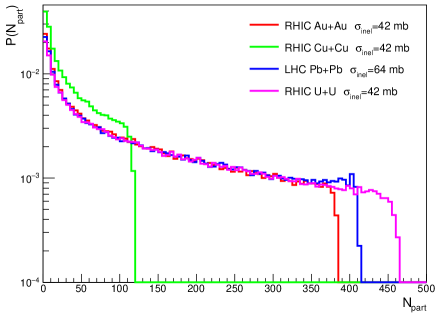
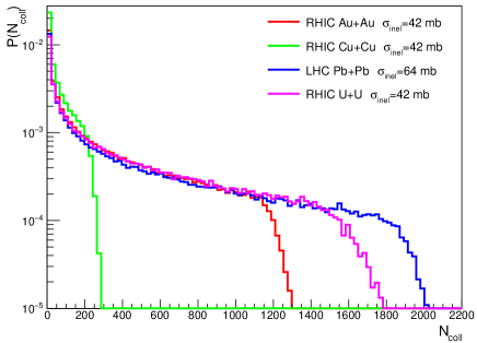
To provide example applications of this code, 100k events were generated for Cu+Cu, Au+Au and U+U at RHIC energies ($\sqrt{s_{\scriptscriptstyle{{\rm NN}}}}=42$ mb), and Pb+Pb at LHC beam energy ($\sqrt{s_{\scriptscriptstyle{{\rm NN}}}}=64$ mb) using the runAndSaveNtuple() function. The resulting ntuples were used to plot the distributions of $N_{\rm part}$ and $N_{\rm coll}$, shown in Fig. 3.

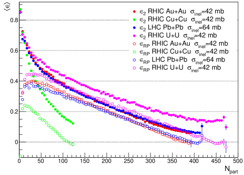
Using the event-by-event quantities, one can construct combinations of moments like eccentricity :

• Reaction-plane eccentricity $\epsilon_{\rm RP}$

  $$\mbox{$\epsilon_{\rm RP}$}=\frac{\text{VarY}-\text{VarX}}{\text{VarY}+\text{VarX}}$$ (7)

• Participant-plane eccentricity $\epsilon_{\rm part}$

  $$\mbox{$\epsilon_{\rm part}$}=\frac{\sqrt{(\text{VarY}-\text{VarX})^{2}+4\text{VarXY}^{2}}}{\text{VarY}+\text{VarX}}$$ (8)

which are shown in Fig. 4 for different systems.

IV Summary

Glauber Model calculations are commonly used by heavy-ion physics experiments to study the initial state configurations of nuclear matter. This document describes the updated implementation (v2) of the Monte Carlo based Glauber Model calculation, which originally was used by the PHOBOS collaboration. The main improvement w.r.t. the earlier version Alver:2008aq are the inclusion of Tritium, Helium-3, and Uranium, as well as the treatment of deformed nuclei and Glauber-Gribov fluctuations of the proton in p+A collisions. The code, accessible online, can be used within user code or in a standalone mode allowing analysis of various distributions. The authors welcome comments on the code and suggestions on how to make it more useful to both experimentalists and theorists.

References

- (1) B. Alver, M. Baker, C. Loizides and P. Steinberg (2008), arXiv:0805.4411.
- (2) M.L. Miller, K. Reygers, S.J. Sanders, and P. Steinberg, Ann. Rev. Nucl. Part. Sci. 57 (2007) 205, arXiv:nucl-ex/0701025.
- (3) B.Alver et al. [PHOBOS Collaboration], Phys. Rev. C 77 (2008) 014906, arXiv:0711.3724.
- (4) M. Rybczynski, G. Stefanek, W. Broniowski and P. Bozek, Comput. Phys. Commun. 185, 1759 (2014), arXiv:1310.5475.
- (5) C. Loizides, J. Kamin and D. d’Enterria, arXiv:1710.07098.
- (6) H. De Vries, C.W. De Jager, and C. De Vries, Atom. Data Nucl. Data Tabl. 36 495 (1987).
- (7) C. W. De Jager, H. De Vries and C. De Vries, Atom. Data Nucl. Data Tabl. 14, 479 (1974).
- (8) L. Hulthen and M. Sugawara, Handbuch der Physik 39 1 (1957).
- (9) S.S. Adler et al. [PHENIX Collaboration], Phys. Rev. Lett. 91 072303 (2003), arXiv:nucl-ex/0306021.
- (10) S. S. Adler et al. [PHENIX Collaboration], Phys. Rev. C 74, 024904 (2006), arXiv:nucl-ex/0603010.
- (11) J. L. Nagle et al., Phys. Rev. Lett. 113 (2014) 112301, arXiv:1312.4565 [nucl-th].
- (12) S. H. Lim et al., arXiv:1812.08096 [nucl-th].
- (13) J. L. Nagle and W. A. Zajc arXiv:1808.01276.
- (14) T. Hirano and Y. Nara, Phys. Rev. C 79, 064904 (2009), arXiv:0904.4080.
- (15) Q. Y. Shou et al. Phys. Lett. B 749 (2015) 215, arXiv:1409.8375 [nucl-th].
- (16) R. Hofstadter et al., Rev. Mod. Phys. 28 (1956) 214.
- (17) P. Möller, J.R. Nix, W.D. Myers and W.J. Swiatecki, Atomic Data and Nuclear Data Tables 59 185 (1995).
- (18) R. Corke and T. Sjostrand, JHEP 1105, 009 (2011), arXiv:1101.5953.
- (19) K. Tsukada et al., Phys. Rev. Lett. 118 (2017) 262501 [arXiv:1703.04278].
- (20) W. Fischer et al. Z. Physik 270 (1974) 270 113
- (21) ALICE Collaboration, public note, ALICE-PUBLIC-2018-003 (2018).
- (22) U. W. Heinz and A. Kuhlman, Phys. Rev. Lett. 94, 132301 (2005), arXiv:nucl-th/0411054
- (23) See https://twiki.cern.ch/twiki/bin/view/Main/LHCGlauberBaseline.
- (24) See http://root.cern.ch for installation files and documentation.
- (25) See the TGlauberMC page on HepForge (http://www.hepforge.org/downloads/tglaubermc) for the most recent TGlauberMC release (latest version v2.7).
- (26) M. Alvioli and M. Strikman, Phys. Lett. B 722, 347 (2013) arXiv:1301.0728.
- (27) G. Aad et al. [ATLAS Collaboration], Eur. Phys. J. C 76 (2016) 199, arXiv:1508.00848.