Leptogenesis and the Higgs Portal

Matthias Le Dall and Adam Ritz Department of Physics and Astronomy, University of Victoria, Victoria, BC, V8P 5C2 Canada
(August 2014)
Abstract

We study the impact on leptogenesis of Higgs portal couplings to a new scalar singlet. These couplings open up additional CP𝐶𝑃CP-violating decay channels for the higher mass singlet neutrinos N2subscript𝑁2N_{2} and N3subscript𝑁3N_{3}. We analyze the simplest case of two-level N1N2subscript𝑁1subscript𝑁2N_{1}-N_{2} leptogenesis, including significant mass hierarchies, in which the CP𝐶𝑃CP asymmetry is generated in part by singlet-mediated decays of N2subscript𝑁2N_{2}. For these models, provided the lightest singlet neutrino N1subscript𝑁1N_{1} is sufficiently weakly coupled to avoid excessive washout, its mass scale is not directly constrained by the Davidson-Ibarra bound.

1 Introduction

The discovery of neutrino oscillations Mohapatra et al. (2007); *deGouvea:2004gd; *GonzalezGarcia:2002dz, and thus small neutrino masses Capozzi et al. (2014); *Fogli:2012ua; *GonzalezGarcia:2012sz; *Tortola:2012te, provides motivation for leptogenesis Fukugita and Yanagida (1986); Luty (1992); Buchmuller et al. (2005a); Davidson et al. (2008); Blanchet and Di Bari (2012) as a simple, and seemingly generic, mechanism for producing the observed baryon asymmetry in the universe. The simplest UV completions of the dimension five Weinberg operator HLHL𝐻𝐿𝐻𝐿HLHL Weinberg (1979), which contribute to neutrino masses, naturally incorporate heavy degrees of freedom with allowed CP𝐶𝑃CP-violating couplings, whose out-of-equilibrium decay can generate a lepton asymmetry. Standard Model (SM) sphaleron processes can then equilibrate BL𝐵𝐿B-L above the weak scale, resulting in the required late time asymmetry in baryon number Klinkhamer and Manton (1984); *Kuzmin:1985mm; *Arnold:1987mh; *Arnold:1987zg; *Harvey:1990qw.

Beyond the clear possibility to test the Majorana nature of neutrinos through neutrinoless double beta decay Racah (1937); *Furry:1939qr; *Vergados:2012xy; *Bilenky:2012qi, the high-scale nature of leptogenesis - characterized for example by the Davidson-Ibarra bound Davidson and Ibarra (2002) - and the lack of model-independent links between the high-scale and low-scale manifestations of CP𝐶𝑃CP-violation, renders the mechanism feasible but hard to test Branco et al. (2012). This has motivated continuing study of variations of this general framework which may be placed under further experimental scrutiny, particularly those that allow a lowering of the scale (see e.g. Hambye (2002); *Fong:2013gaa; *Tsuyuki:2014aia; *Ma:2006ci). This turns out to be quite difficult for the basic reason that the asymmetries generated by loop-level decays are counteracted by similar washout processes from two-to-two scattering. Lowering the scale at which the asymmetry is generated means a lower Hubble expansion rate, and thus more scattering processes will be in equilibrium and able to efficiently cancel the asymmetry. The conclusion being that it becomes increasingly difficult to find viable scenarios which operate at or close to the weak scale; an exception is the case of resonant decays Pilaftsis and Underwood (2004); *Pilaftsis:2005rv.

From a theoretical perspective, the simplest realization of leptogenesis, with heavy right-handed (RH), i.e. singlet, Majorana neutrinos, involves one of the few renormalizable interactions between the SM and a neutral hidden (or dark) sector. The RH neutrino coupling is described by the Langrangian,

=SM+iN¯iγμμNiλjiN¯iPLLjH12MiN¯icNi+h.c.formulae-sequencesubscriptSM𝑖subscript¯𝑁𝑖superscript𝛾𝜇subscript𝜇subscript𝑁𝑖subscript𝜆𝑗𝑖subscript¯𝑁𝑖subscript𝑃𝐿subscript𝐿𝑗𝐻12subscript𝑀𝑖subscriptsuperscript¯𝑁𝑐𝑖subscript𝑁𝑖𝑐{\cal L}={\cal L}_{\rm SM}+i\overline{N}_{i}\gamma^{\mu}\partial_{\mu}N_{i}-\lambda_{ji}\overline{N}_{i}P_{L}L_{j}\cdot H-\frac{1}{2}M_{i}\overline{N}^{c}_{i}N_{i}+h.c. (1)

The class of UV complete relevant or marginal interactions of the type characterized by λjisubscript𝜆𝑗𝑖\lambda_{ji}, known as portals, is very small. If we require no additional states, the list contains this right-handed neutrino coupling, λN¯LH𝜆¯𝑁𝐿𝐻\lambda\bar{N}L\cdot H, the coupling of a scalar singlet to the Higgs, (βS+λS2)HH𝛽𝑆𝜆superscript𝑆2superscript𝐻𝐻(\beta S+\lambda S^{2})H^{\dagger}H, and kinetic mixing of a U(1) vector with hypercharge, κVμνBμν𝜅subscript𝑉𝜇𝜈superscript𝐵𝜇𝜈\kappa V_{\mu\nu}B^{\mu\nu}. Since the coefficients of these operators are unsuppressed by any heavy new physics scale, they are a natural place to look for signs of new short-distance physics. Couplings to a hidden sector are also motivated by our other primary piece of empirical evidence for new physics, namely dark matter, and thus these portals have been the focus of considerable recent attention Essig et al. (2013).

In this paper, we explore the minimal extension of ‘standard’ leptogenesis incorporating the Higgs portal coupling, which is now subject to direct experimental probes at the LHC. The relevant and marginal interactions then include,

\displaystyle{\cal L} =SM+iN¯iγμμNiλjiN¯iPLLjH12MiN¯icNiabsentsubscriptSM𝑖subscript¯𝑁𝑖superscript𝛾𝜇subscript𝜇subscript𝑁𝑖subscript𝜆𝑗𝑖subscript¯𝑁𝑖subscript𝑃𝐿subscript𝐿𝑗𝐻12subscript𝑀𝑖subscriptsuperscript¯𝑁𝑐𝑖subscript𝑁𝑖\displaystyle={\cal L}_{\rm SM}+i\overline{N}_{i}\gamma^{\mu}\partial_{\mu}N_{i}-\lambda_{ji}\overline{N}_{i}P_{L}L_{j}\cdot H-\frac{1}{2}M_{i}\overline{N}^{c}_{i}N_{i}
βSHHαijSN¯icPLNj+h.c.+formulae-sequence𝛽𝑆superscript𝐻𝐻subscript𝛼𝑖𝑗𝑆subscriptsuperscript¯𝑁𝑐𝑖subscript𝑃𝐿subscript𝑁𝑗𝑐\displaystyle\qquad\qquad-\beta SH^{\dagger}H-\alpha_{ij}S\overline{N}^{c}_{i}P_{L}N_{j}+h.c.+\cdots (2)

We have not shown the quartic Higgs portal coupling here as it will not play a significant role, other than for the full scalar potential, but have added the allowed Majoron coupling αijsubscript𝛼𝑖𝑗\alpha_{ij} between the scalar S𝑆S and Nisubscript𝑁𝑖N_{i}. The ensuing scenario for baryogenesis will be referred to as Higgs Portal Leptogenesis (HPL).

As we discuss below, this minimal extension is sufficient to open up new CP𝐶𝑃CP-violating decay channels for the next-to-lightest singlet neutrino N2subscript𝑁2N_{2} (and N3subscript𝑁3N_{3}). These new channels also decouple the source of the CP𝐶𝑃CP-asymmetry from the seesaw contribution to the light neutrino mass. Consequently, leptogenesis can be viable in a wider mass range, and in particular when the lightest singlet neutrino is very light, e.g. below the sphaleron threshold. To analyze the impact of the new decay channels, we study the case of two-level N1N2subscript𝑁1subscript𝑁2N_{1}-N_{2} leptogenesis in detail, paying attention to the washout induced by scattering associated with N1subscript𝑁1N_{1} and the additional scalar. In minimal leptogenesis, these two-to-two processes are generally negligible as the neutrino abundance is Boltzmann suppressed. This is not necessarily the case for N2,1subscript𝑁21N_{2,1} scattering mediated by the hidden sector, and washout would be problematic if N1subscript𝑁1N_{1} were in equilibrium for an extended period. Nonetheless, we find that there are viable regions of parameter space in which N1subscript𝑁1N_{1} is parametrically light, but also very weakly coupled, in which the lepton asymmetry generated by N2subscript𝑁2N_{2} decays survives to provide the observed baryon abundance (see e.g. Engelhard et al. (2007); *Vives:2005ra; *DiBari:2005st; *Blanchet:2006dq). The possibility of effectively decoupling N1subscript𝑁1N_{1} from its normally dominant role in leptogenesis, and having it be parametrically light and experimentally accessible Hambye (2002); Engelhard et al. (2007), is one of the interesting features of HPL.

The rest of the paper is organized as follows. In Section 2, we outline the model and determine the additional contributions to the CP𝐶𝑃CP asymmetry from the hidden sector. Since the hidden sector contributions enter only through the decays of the next-to-lightest singlet neutrinos, in Section 3 we turn to the Boltzmann evolution of the coupled N1N2subscript𝑁1subscript𝑁2N_{1}-N_{2} system, and study in some detail the important role of N1subscript𝑁1N_{1}-mediated two-to-two scattering in washing out the N2subscript𝑁2N_{2}-generated asymmetry. Section 4 presents a number of results for the final lepton asymmetry in different mass regimes. The new hidden sector contributions to the CP𝐶𝑃CP asymmetry are crucial in allowing a lowering of the overall mass scale without violating the Davidson-Ibarra bound. We conclude in Section 5, while a series of Appendices contain further technical details.

2 Higgs Portal and the CP𝐶𝑃CP-asymmetry

2.1 The Model

Our focus in this paper will be a minimal extension of conventional leptogenesis, which adds a scalar singlet S𝑆S along with the right-handed singlet neutrinos Nisubscript𝑁𝑖N_{i}. This opens up the Higgs and neutrino portals and, significantly, allows for a new CP𝐶𝑃CP-odd source in the hidden sector. CP𝐶𝑃CP-violation is of course a central ingredient in leptogenesis, as it is in any theory of matter genesis according to the Sakharov conditions Sakharov (1967). The portal couplings in the Lagrangian (2) include

portals=λjiN¯iPLLjHβSHH(12Miδij+αijS)N¯icPLNj+h.c.+formulae-sequencesubscriptportalssubscript𝜆𝑗𝑖subscript¯𝑁𝑖subscript𝑃𝐿subscript𝐿𝑗𝐻𝛽𝑆superscript𝐻𝐻12subscript𝑀𝑖subscript𝛿𝑖𝑗subscript𝛼𝑖𝑗𝑆subscriptsuperscript¯𝑁𝑐𝑖subscript𝑃𝐿subscript𝑁𝑗𝑐{\cal L}_{\rm portals}=-\lambda_{ji}\overline{N}_{i}P_{L}L_{j}\cdot H-\beta SH^{\dagger}H-\left(\frac{1}{2}M_{i}\delta_{ij}+\alpha_{ij}S\right)\overline{N}^{c}_{i}P_{L}N_{j}+h.c.+\cdots (3)

The Higgs portal coupling β𝛽\beta is one part of the full scalar potential V(H,S)𝑉𝐻𝑆V(H,S), and necessarily breaks any SS𝑆𝑆S\rightarrow-S symmetry. Thus, determining the vacuum structure requires a separate analysis incorporating thermal corrections. This potential has been studied in detail elsewhere Profumo et al. (2007); *Ahriche:2007jp; *Biswas:2011td, and here we simply assume that the parameters are chosen to ensure viable electroweak symmetry breaking, and importantly that S=0delimited-⟨⟩𝑆0\langle S\rangle=0. The possibility of a more complex behaviour of Sdelimited-⟨⟩𝑆\langle S\rangle, which modifies the effective RHN mass is nonetheless interesting, and will be discussed further in the concluding section.

In minimal leptogenesis, the Yukawa couplings λ𝜆\lambda determine both the light neutrino mass spectrum and the CP𝐶𝑃CP-asymmetry generated in RH neutrino decays Covi et al. (1996); *Roulet:1997xa; *Buchmuller:1997yu; *Pilaftsis:1997jf. Opening the Higgs portal allows these two physical phenomena to be decoupled, with the Majoron coupling αijsubscript𝛼𝑖𝑗\alpha_{ij} providing a new CP𝐶𝑃CP-odd source that is unconstrained (for S=0delimited-⟨⟩𝑆0\langle S\rangle=0) by the light neutrino mass spectrum. In the Lagrangian (3), a unitary rotation has been used to diagonalize the RH neutrino mass matrix MijMiδijsubscript𝑀𝑖𝑗subscript𝑀𝑖subscript𝛿𝑖𝑗M_{ij}\rightarrow M_{i}\delta_{ij}. The Majorana nature of Ni=Nicsubscript𝑁𝑖superscriptsubscript𝑁𝑖𝑐N_{i}=N_{i}^{c} ensures that Mijsubscript𝑀𝑖𝑗M_{ij} is symmetric, and for n𝑛n flavors the diagonalization leaves Misubscript𝑀𝑖M_{i} as n𝑛n real mass eigenvalues Bigi and Sanda (2000); *Doi:1985dx. In general, the corresponding rotation simply rearranges the n(n+1)/2𝑛𝑛12n(n+1)/2 phases in the symmetric matrix αijsubscript𝛼𝑖𝑗\alpha_{ij}, which is thus a physical CP𝐶𝑃CP-odd source in addition to the neutrino Yukawa λijsubscript𝜆𝑖𝑗\lambda_{ij}.111The coupling αijSN¯icPLNj+h.cformulae-sequencesubscript𝛼𝑖𝑗𝑆subscriptsuperscript¯𝑁𝑐𝑖subscript𝑃𝐿subscript𝑁𝑗𝑐\alpha_{ij}S\overline{N}^{c}_{i}P_{L}N_{j}+h.c is more commonly used to generate the right-handed neutrino masses Misubscript𝑀𝑖M_{i} by having S𝑆S develop a vev Sdelimited-⟨⟩𝑆\langle S\rangle, spontaneously breaking a global lepton number symmetry. In such cases where an explicit mass term Mijsubscript𝑀𝑖𝑗M_{ij} is forbidden, the matrix αijsubscript𝛼𝑖𝑗\alpha_{ij} can be be made real and diagonal.

2.2 CP Asymmetry

In leptogenesis, the CP𝐶𝑃CP-asymmetry arises from RH neutrino (RHN) decays to leptons, NLH𝑁𝐿𝐻N\rightarrow LH and NL¯H¯𝑁¯𝐿¯𝐻N\rightarrow\overline{L}\overline{H}, and is measured by ϵisubscriptitalic-ϵ𝑖\epsilon_{i},

ϵiΓ(NiLH)Γ(NiL¯H¯)Γi.subscriptitalic-ϵ𝑖Γsubscript𝑁𝑖𝐿𝐻Γsubscript𝑁𝑖¯𝐿¯𝐻subscriptΓ𝑖\epsilon_{i}\equiv\frac{\Gamma(N_{i}\rightarrow LH)-\Gamma(N_{i}\rightarrow\overline{L}\overline{H})}{\Gamma_{i}}. (4)

In the denominator, the Nisubscript𝑁𝑖N_{i} decay rate is calculated at tree level, and reads

Γik,α,β(Γ(NiLkαHβ)+Γ(NiLkαHβ¯))=(λλ)ii8πMi,subscriptΓ𝑖subscript𝑘𝛼𝛽Γsubscript𝑁𝑖subscriptsuperscript𝐿𝛼𝑘superscript𝐻𝛽Γsubscript𝑁𝑖¯superscriptsubscript𝐿𝑘𝛼superscript𝐻𝛽subscriptsuperscript𝜆𝜆𝑖𝑖8𝜋subscript𝑀𝑖\Gamma_{i}\equiv\sum_{k,\alpha,\beta}\left(\Gamma(N_{i}\rightarrow L^{\alpha}_{k}H^{\beta})+\Gamma(N_{i}\rightarrow\overline{L_{k}^{\alpha}H^{\beta}})\right)=\frac{(\lambda^{\dagger}\lambda)_{ii}}{8\pi}M_{i}, (5)

where the lepton family index, k=1,2,3𝑘123k=1,2,3 stands for the electron, muon and tau families respectively. The α,β=1,2formulae-sequence𝛼𝛽12\alpha,\beta=1,2 indices denote the components of the SU(2) lepton and Higgs doublets L=(νlel)T𝐿superscriptsubscript𝜈𝑙subscript𝑒𝑙𝑇L=(\nu_{l}\quad e_{l})^{T} and H=(H+H0)T𝐻superscriptsuperscript𝐻superscript𝐻0𝑇H=(H^{+}\quad H^{0})^{T}. If we schematically write the decay amplitude as i=Γ0+Γ1I𝑖subscriptΓ0subscriptΓ1𝐼i\mathcal{M}=\Gamma_{0}+\Gamma_{1}I, with Γ0,1subscriptΓ01\Gamma_{0,1} the tree and loop level combinations of coupling constants, and I𝐼I the loop function, then the decay amplitude for the antiparticle is i¯=Γ0+Γ1I𝑖¯superscriptsubscriptΓ0superscriptsubscriptΓ1𝐼i\overline{\mathcal{M}}=\Gamma_{0}^{*}+\Gamma_{1}^{*}I, while the decay rates Γ(NiLH)Γsubscript𝑁𝑖𝐿𝐻\Gamma(N_{i}\rightarrow LH) and Γ(NiLH¯)Γsubscript𝑁𝑖¯𝐿𝐻\Gamma(N_{i}\rightarrow\overline{LH}) are proportional to |i|2superscript𝑖2|i\mathcal{M}|^{2} and |i¯|2superscript𝑖¯2|i\overline{\mathcal{M}}|^{2} respectively. At tree level, the difference vanishes, but at the loop level, the CP𝐶𝑃CP-asymmetry takes the schematic form

ϵi2Im{Γ0Γ1}|Γ0|2Im{I}.similar-tosubscriptitalic-ϵ𝑖2ImsubscriptΓ0superscriptsubscriptΓ1superscriptsubscriptΓ02Im𝐼\epsilon_{i}\sim 2\frac{\text{Im}\{\Gamma_{0}\Gamma_{1}^{*}\}}{|\Gamma_{0}|^{2}}\text{Im}\{I\}. (6)

Thus, at least for two-body decays, the CP𝐶𝑃CP-asymmetry requires loops, and a phase in the loop function itself. In standard leptogenesis, only the Yukawa λijsubscript𝜆𝑖𝑗\lambda_{ij} allows for this decay channel, and can accommodate CP-violation. In Higgs Portal Leptogenesis, additional lepton number violating and CP𝐶𝑃CP-violating sources are present in the theory, specifically the αijsubscript𝛼𝑖𝑗\alpha_{ij} coupling as discussed above. As a result, additional loop-induced decay channels open up, as displayed in Fig. 1.

Refer to caption

Figure 1: Two hidden sector decay channels for RHN that contribute to the CP𝐶𝑃CP asymmetry. The superscripts ‘v’, and ‘w’ stand for the vertex and wave function diagrams.

The corresponding CP𝐶𝑃CP-asymmetries will be discussed in the following subsections. We utilize the Majorana Feynman rules Gates and Kowalski (1988); *Denner:1992me; *Denner:1992vza for the RH neutrinos, and determine the imaginary parts of the loop functions using the standard Cutkosky rules Cutkosky (1960).

Vertex Corrections: 2-body final states

The contribution of the diagram iv𝑖superscript𝑣i\mathcal{M}^{v} to the asymmetry is

ϵiv=4j(Im{(λλ)jiβαij}(λλ)iiMi Im{IjLL}+Im{(λλ)jiβαij}(λλ)iiMiIm{IjRL}),superscriptsubscriptitalic-ϵ𝑖𝑣4subscript𝑗Imsubscriptsuperscript𝜆𝜆𝑗𝑖𝛽subscript𝛼𝑖𝑗subscriptsuperscript𝜆𝜆𝑖𝑖subscript𝑀𝑖 Imsubscript𝐼𝑗𝐿𝐿Imsubscriptsuperscript𝜆𝜆𝑗𝑖𝛽superscriptsubscript𝛼𝑖𝑗subscriptsuperscript𝜆𝜆𝑖𝑖subscript𝑀𝑖Imsubscript𝐼𝑗𝑅𝐿\epsilon_{i}^{v}=4\sum_{j}\left(\frac{\text{Im}\{(\lambda^{\dagger}\lambda)_{ji}\beta\alpha_{ij}\}}{(\lambda^{\dagger}\lambda)_{ii}M_{i}}\text{ Im}\{I_{jLL}\}+\frac{\text{Im}\{(\lambda^{\dagger}\lambda)_{ji}\beta\alpha_{ij}^{*}\}}{(\lambda^{\dagger}\lambda)_{ii}M_{i}}\text{Im}\{I_{jRL}\}\right), (7)

where IjLLsubscript𝐼𝑗𝐿𝐿I_{jLL} and IjRLsubscript𝐼𝑗𝑅𝐿I_{jRL} are loop function integrals. The vertex contribution splits into two halves, proportional to Im{IjLL}Imsubscript𝐼𝑗𝐿𝐿\text{Im}\{I_{jLL}\} and Im{IjRL}Imsubscript𝐼𝑗𝑅𝐿\text{Im}\{I_{jRL}\}, corresponding to the mixing of the left- and right- chiralities of the Majorana fermions along the fermion lines, effectively leading to the two chirality chains

νR(RH)νRC(LH)L(LH),νRC(LH)νRC(LH)L(LH).formulae-sequencesubscript𝜈𝑅RHsuperscriptsubscript𝜈𝑅𝐶LH𝐿LHsuperscriptsubscript𝜈𝑅𝐶LHsuperscriptsubscript𝜈𝑅𝐶LH𝐿LH\begin{split}&\nu_{R}(\text{RH})\longrightarrow\nu_{R}^{C}(\text{LH})\longrightarrow L(\text{LH}),\\ &\nu_{R}^{C}(\text{LH})\longrightarrow\nu_{R}^{C}(\text{LH})\longrightarrow L(\text{LH}).\end{split} (8)

Because the final leptons (assumed massless) have a definite chirality, the Yukawa coupling forces the next-to-last neutrino to be of the same chirality as the final lepton, left-handed. The functions IjLLsubscript𝐼𝑗𝐿𝐿I_{jLL} and IjRLsubscript𝐼𝑗𝑅𝐿I_{jRL} correspond to the L-L-L and R-L-L chains respectively. The reason why the chirality chains do not combine, owes to the fact that αijsubscript𝛼𝑖𝑗\alpha_{ij} is neither real nor diagonal. In the vertex contribution, there are three possible cuts which lead to an imaginary part: cuts along the S/N𝑆𝑁S/N lines, the H/S𝐻𝑆H/S lines and the H/N𝐻𝑁H/N lines, each of which contains the two chirality chain contributions. Thus, each chirality chain function, Im{IjLL}Imsubscript𝐼𝑗𝐿𝐿\text{Im}\{I_{jLL}\} and Im{IjRL}Imsubscript𝐼𝑗𝑅𝐿\text{Im}\{I_{jRL}\} is the sum,

Im{I}=Im{I}S/N+Im{I}H/S+Im{I}H/N.Im𝐼Imsuperscript𝐼𝑆𝑁Imsuperscript𝐼𝐻𝑆Imsuperscript𝐼𝐻𝑁\text{Im}\{I\}=\text{Im}\{I\}^{S/N}+\text{Im}\{I\}^{H/S}+\text{Im}\{I\}^{H/N}. (9)

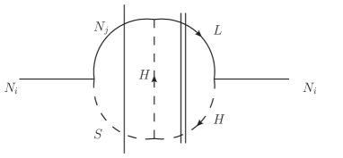
It will be convenient to graphically represent the interference terms in ||2superscript2|{\cal M}|^{2} which contribute to the imaginary part in the form of bubble diagrams. For now we focus on the N/S𝑁𝑆N/S cut which is shown in Fig. 2 (the full set of cuts is presented later in Fig. 4). The double line indicates external lines that are on-shell by definition in ||2superscript2|{\cal M}|^{2}, in this case the final lepton and Higgs, while the single line shows the Cutkosky-cut. According to the Cutkosky rules, the N/S𝑁𝑆N/S cut is given by

Refer to caption

Refer to caption

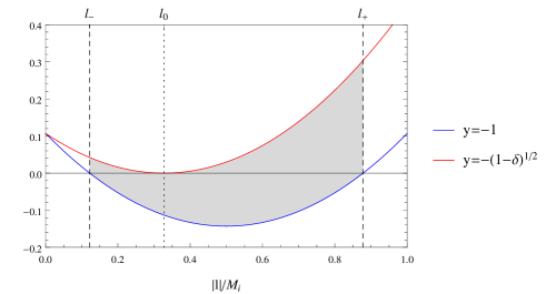
Figure 2: The left plot graphically represents the N/S𝑁𝑆N/S cut. The right figure exhibits the quadratic constraint in Eq. (11). The vertical dashed lines represent the momentum |l|𝑙|\vec{l}| upper and lower bounds, |l|±=Mi(1±δ)/2subscript𝑙plus-or-minussubscript𝑀𝑖plus-or-minus1𝛿2|\vec{l}|_{\pm}=M_{i}(1\pm\sqrt{\delta})/2, which become |l|0=Mi1δ/2subscript𝑙0subscript𝑀𝑖1𝛿2|\vec{l}|_{0}=M_{i}\sqrt{1-\delta}/2 at y=1δ𝑦1𝛿y=-\sqrt{1-\delta}. The imaginary part of the vertex correction is non-zero contributions only from the gray area.
Im{ILL}S/N=2π2d4l(2π)4lkl2δ((l+k)2Mj2)δ((l+kp)2mS2)×Θ(p0l0k0)Θ(k0+l0).Imsuperscriptsubscript𝐼𝐿𝐿𝑆𝑁2superscript𝜋2superscript𝑑4𝑙superscript2𝜋4𝑙𝑘superscript𝑙2𝛿superscript𝑙𝑘2superscriptsubscript𝑀𝑗2𝛿superscript𝑙𝑘𝑝2superscriptsubscript𝑚𝑆2Θsuperscript𝑝0superscript𝑙0superscript𝑘0Θsuperscript𝑘0superscript𝑙0\begin{split}\text{Im}\{I_{LL}\}^{S/N}=2\pi^{2}\int\frac{d^{4}l}{(2\pi)^{4}}\frac{l\cdot k}{l^{2}}&\delta((l+k)^{2}-M_{j}^{2})\delta((l+k-p)^{2}-m_{S}^{2})\\ &\times\Theta(p^{0}-l^{0}-k^{0})\Theta(k^{0}+l^{0}).\end{split} (10)

The delta functions impose the on-shell condition for the N/S𝑁𝑆N/S lines, and the Heaviside functions ΘΘ\Theta require these on-shell lines to be physical (timelike) processes. In other words, imposing positivity of the energies p0l0k0superscript𝑝0superscript𝑙0superscript𝑘0p^{0}-l^{0}-k^{0} and k0+l0superscript𝑘0superscript𝑙0k^{0}+l^{0}, requires that the cut diagram corresponds to the decay NiNjSsubscript𝑁𝑖subscript𝑁𝑗𝑆N_{i}\rightarrow N_{j}S followed by the scattering NjSLHsubscript𝑁𝑗𝑆𝐿𝐻N_{j}S\rightarrow LH. Combining the energy constraints also restricts the individual energies l0=Mi(rjiσi)/2superscript𝑙0subscript𝑀𝑖subscript𝑟𝑗𝑖subscript𝜎𝑖2l^{0}=M_{i}(r_{ji}-\sigma_{i})/2, and Mi/2>l0>Mi/2subscript𝑀𝑖2superscript𝑙0subscript𝑀𝑖2M_{i}/2>l^{0}>-M_{i}/2. The on-shell conditions in turn, imply the quadratic constraint on the three momentum l𝑙\vec{l}

|l|2+Mi|l|yMi24(δ(1,rji,σi)1)=0,superscript𝑙2subscript𝑀𝑖𝑙𝑦superscriptsubscript𝑀𝑖24𝛿1subscript𝑟𝑗𝑖subscript𝜎𝑖10|\vec{l}|^{2}+M_{i}|\vec{l}|y-\frac{M_{i}^{2}}{4}\Big{(}\delta(1,r_{ji},\sigma_{i})-1\Big{)}=0, (11)

where we have introduced the shorthand notations

rji=Mj2Mi2,σi=mS2Mi2,δ(a,b,c)=(abc)24bc,y=cosθ,formulae-sequencesubscript𝑟𝑗𝑖superscriptsubscript𝑀𝑗2superscriptsubscript𝑀𝑖2formulae-sequencesubscript𝜎𝑖superscriptsubscript𝑚𝑆2superscriptsubscript𝑀𝑖2formulae-sequence𝛿𝑎𝑏𝑐superscript𝑎𝑏𝑐24𝑏𝑐𝑦𝜃r_{ji}=\frac{M_{j}^{2}}{M_{i}^{2}},\quad\sigma_{i}=\frac{m_{S}^{2}}{M_{i}^{2}},\quad\delta(a,b,c)=(a-b-c)^{2}-4bc,\quad y=\cos\theta, (12)

For simplicity below, δ𝛿\delta without specified variables will implicitly be understood to mean δ(1,rji,σi)𝛿1subscript𝑟𝑗𝑖subscript𝜎𝑖\delta(1,r_{ji},\sigma_{i}), unless stated otherwise. The angle θ𝜃\theta lies between the 3-momenta l𝑙\vec{l} and k𝑘\vec{k}. The combined constraints on l0superscript𝑙0l^{0} given above imply the equivalent constraint, 1>rjiσi>11subscript𝑟𝑗𝑖subscript𝜎𝑖11>r_{ji}-\sigma_{i}>-1. Since the kinematics must allow the decay NiNjSsubscript𝑁𝑖subscript𝑁𝑗𝑆N_{i}\rightarrow N_{j}S, the latter constraint requires that 1>rji+σi1subscript𝑟𝑗𝑖subscript𝜎𝑖1>\sqrt{r_{ji}}+\sqrt{\sigma_{i}}. Importantly, we observe that the diagram only has an imaginary part for decays of the next-to-lightest neutrinos. Similarly, the imaginary part is non-vanishing provided the quadratic equation for |l|𝑙|\vec{l}| in (11) has real solutions, thus imposing the condition δ>0𝛿0\delta>0, here again, satisfied if 1>rji+σi1subscript𝑟𝑗𝑖subscript𝜎𝑖1>\sqrt{r_{ji}}+\sqrt{\sigma_{i}}. The l0superscript𝑙0l^{0} integration is trivial since its value is uniquely fixed. As usual, the remaining integration over l𝑙\vec{l} is split into the radial and angular part. In spherical coordinates with k𝑘\vec{k} along the z-axis, the azimuthal angle ϕitalic-ϕ\phi trivially integrates to 2π2𝜋2\pi, and θ𝜃\theta corresponds to the inclination angle of the spherical coordinate system. The leftover integrals over y𝑦y and |l|𝑙|\vec{l}| are not independent because of the constraint (11). That constraint has been plotted in Fig. 2, where we see that the kinematics are constrained to the ranges 1y1δ1𝑦1𝛿-1\leqslant y\leqslant-\sqrt{1-\delta} and Mi/2(1δ)|l|Mi/2(1+δ)subscript𝑀𝑖21𝛿𝑙subscript𝑀𝑖21𝛿M_{i}/2\left(1-\sqrt{\delta}\right)\leqslant|\vec{l}|\leqslant M_{i}/2\left(1+\sqrt{\delta}\right). The integration is nonvanishing within this range, leading to the result,

Im{ILL}N/S=132π[δ+rjilog(δ+4rjiσiδδ+4rjiσi+δ)],1rji+σi.formulae-sequenceImsuperscriptsubscript𝐼𝐿𝐿𝑁𝑆132𝜋delimited-[]𝛿subscript𝑟𝑗𝑖𝛿4subscript𝑟𝑗𝑖subscript𝜎𝑖𝛿𝛿4subscript𝑟𝑗𝑖subscript𝜎𝑖𝛿1subscript𝑟𝑗𝑖subscript𝜎𝑖\text{Im}\{I_{LL}\}^{N/S}=\frac{1}{32\pi}\left[-\sqrt{\delta}+r_{ji}\log\left(\frac{\sqrt{\delta+4r_{ji}\sigma_{i}}-\sqrt{\delta}}{\sqrt{\delta+4r_{ji}\sigma_{i}}+\sqrt{\delta}}\right)\right],\quad 1\geqslant\sqrt{r_{ji}}+\sqrt{\sigma_{i}}. (13)

Similar steps lead to the other chirality chain function, Im{IjRL}N/SImsuperscriptsubscript𝐼𝑗𝑅𝐿𝑁𝑆\text{Im}\{I_{jRL}\}^{N/S}, for the N/S𝑁𝑆N/S cut,

Im{IjRL}N/S=rji32πlog(δ+4rjiσiδδ+4rjiσi+δ),1rji+σi,formulae-sequenceImsuperscriptsubscript𝐼𝑗𝑅𝐿𝑁𝑆subscript𝑟𝑗𝑖32𝜋𝛿4subscript𝑟𝑗𝑖subscript𝜎𝑖𝛿𝛿4subscript𝑟𝑗𝑖subscript𝜎𝑖𝛿1subscript𝑟𝑗𝑖subscript𝜎𝑖\text{Im}\{I_{jRL}\}^{N/S}=\frac{\sqrt{r_{ji}}}{32\pi}\log\left(\frac{\sqrt{\delta+4r_{ji}\sigma_{i}}-\sqrt{\delta}}{\sqrt{\delta+4r_{ji}\sigma_{i}}+\sqrt{\delta}}\right),\quad 1\geqslant\sqrt{r_{ji}}+\sqrt{\sigma_{i}}, (14)

as well as for the H/S𝐻𝑆H/S cuts,

Im{IjRL}H/S=rji32πlog|1rjirji||σi=0,Im{IjLL}H/S=132π(1+rjilog|1rjirji|)|σi=0,\begin{split}&\text{Im}\{I_{jRL}\}^{H/S}=\frac{\sqrt{r_{ji}}}{32\pi}\log\bigg{|}\frac{1-r_{ji}}{r_{ji}}\bigg{|}\Bigg{|}_{\sigma_{i}=0}\quad,\\ &\text{Im}\{I_{jLL}\}^{H/S}=\frac{1}{32\pi}\left(1+r_{ji}\log\bigg{|}\frac{1-r_{ji}}{r_{ji}}\bigg{|}\right)\Bigg{|}_{\sigma_{i}=0},\end{split} (15)

while the H/N𝐻𝑁H/N cut gives a vanishing imaginary part Im{IjLL}H/N=Im{IjRL}H/N=0Imsuperscriptsubscript𝐼𝑗𝐿𝐿𝐻𝑁Imsuperscriptsubscript𝐼𝑗𝑅𝐿𝐻𝑁0\text{Im}\{I_{jLL}\}^{H/N}=\text{Im}\{I_{jRL}\}^{H/N}=0. The notation |σi=0|_{\sigma_{i}=0} means that the imaginary part is only nonzero if σi=0subscript𝜎𝑖0\sigma_{i}=0. Note that the N/S𝑁𝑆N/S cut is divergent in the infrared limit σi=0subscript𝜎𝑖0\sigma_{i}=0, where it is effectively equivalent to the decay NiNjSsubscript𝑁𝑖subscript𝑁𝑗𝑆N_{i}\rightarrow N_{j}S followed by the scattering NjSLHsubscript𝑁𝑗𝑆𝐿𝐻N_{j}S\rightarrow LH mediated by the Higgs in the t-channel. The divergence, due to radiating massless scalars in the infrared collinear limit, is canceled by including the appropriate three-body decays as discussed below.

Vertex Corrections: 3-body final states

Refer to caption


Figure 3: Two 3-body decay diagrams contributing to the CP𝐶𝑃CP-asymmetry at the same order in couplings as the loop-corrected 2-body decays. As discussed in the text, their inclusion is important in ensuring that the full CP𝐶𝑃CP asymmetry is well-defined and free of infrared divergences.

In Fig. 3, we show the two three-body final state amplitudes whose interference develops an imaginary part and contributes to the CP𝐶𝑃CP-asymmetry. The three-body final state CP𝐶𝑃CP-asymmetry ϵi(3)superscriptsubscriptitalic-ϵ𝑖3\epsilon_{i}^{(3)} measures the difference (Γ(NiLHS)Γ(NiL¯H¯S))/(Γ(NiLH,LHS)+Γ(NiLH¯,LH¯S))Γsubscript𝑁𝑖𝐿𝐻𝑆Γsubscript𝑁𝑖¯𝐿¯𝐻𝑆Γsubscript𝑁𝑖𝐿𝐻𝐿𝐻𝑆Γsubscript𝑁𝑖¯𝐿𝐻¯𝐿𝐻𝑆(\Gamma(N_{i}\rightarrow LHS)-\Gamma(N_{i}\rightarrow\overline{L}\overline{H}S))/(\Gamma(N_{i}\rightarrow LH,LHS)+\Gamma(N_{i}\rightarrow\overline{LH},\overline{LH}S)), with the total RHN decay rate in the denominator. The three-body final state decay rate being subdominant due to the reduced phase space, we can approximate ϵi(3)superscriptsubscriptitalic-ϵ𝑖3\epsilon_{i}^{(3)} as

ϵi(3)Γ(NiLHS)Γ(NiL¯H¯S)Γi.similar-to-or-equalssuperscriptsubscriptitalic-ϵ𝑖3Γsubscript𝑁𝑖𝐿𝐻𝑆Γsubscript𝑁𝑖¯𝐿¯𝐻𝑆subscriptΓ𝑖\epsilon_{i}^{(3)}\simeq\frac{\Gamma(N_{i}\rightarrow LHS)-\Gamma(N_{i}\rightarrow\overline{L}\overline{H}S)}{\Gamma_{i}}. (16)

In general, the three-body CP𝐶𝑃CP-asymmetry arises from both iA(iB)𝒪(λ2βα)similar-to𝑖subscript𝐴superscript𝑖subscript𝐵𝒪superscript𝜆2𝛽𝛼i\mathcal{M}_{A}(i\mathcal{M}_{B})^{*}\sim\mathcal{O}(\lambda^{2}\beta\alpha) and |iB|2𝒪(λ2α2)similar-tosuperscript𝑖subscript𝐵2𝒪superscript𝜆2superscript𝛼2|i\mathcal{M}_{B}|^{2}\sim\mathcal{O}(\lambda^{2}\alpha^{2}). Only the former term, which enters at the same order as the vertex contribution, is of interest here. The two contributing cuts through the H𝐻H and the Njsubscript𝑁𝑗N_{j} propagators are represented in Fig. 4 as bubble diagrams. The result is

Refer to caption
Refer to caption
Figure 4: The bubble diagrams enumerating the cuts that contribute to the CP𝐶𝑃CP-asymmetry from both the vertex loop corrections (a) and 3-body final states (b). The external state lines that are on-shell by definition are cut with a double line, while the Cutkosky cuts are shown with a single line.
ϵi(3)=4j(Im{(λλ)jiβαij}(λλ)iiMiIm{jLL}(3)+Im{(λλ)jiβαij}(λλ)iiMiIm{jRL}(3)),superscriptsubscriptitalic-ϵ𝑖34subscript𝑗Imsubscriptsuperscript𝜆𝜆𝑗𝑖𝛽subscript𝛼𝑖𝑗subscriptsuperscript𝜆𝜆𝑖𝑖subscript𝑀𝑖Imsuperscriptsubscript𝑗𝐿𝐿3Imsubscriptsuperscript𝜆𝜆𝑗𝑖𝛽superscriptsubscript𝛼𝑖𝑗subscriptsuperscript𝜆𝜆𝑖𝑖subscript𝑀𝑖Imsuperscriptsubscript𝑗𝑅𝐿3\epsilon_{i}^{(3)}=4\sum_{j}\left(\frac{\text{Im}\left\{(\lambda^{\dagger}\lambda)_{ji}\beta\alpha_{ij}\right\}}{(\lambda^{\dagger}\lambda)_{ii}M_{i}}\text{Im}\{\mathcal{I}_{jLL}\}^{(3)}+\frac{\text{Im}\left\{(\lambda^{\dagger}\lambda)_{ji}\beta\alpha_{ij}^{*}\right\}}{(\lambda^{\dagger}\lambda)_{ii}M_{i}}\text{Im}\{\mathcal{I}_{jRL}\}^{(3)}\right), (17)

with

Im{jLL}(3)=rji32πlog(δ+4rjiσi+2σi+δδ+4rjiσi+2σiδ)132π(1+rjilog|1rjirji|)|σi=0,Im{jRL}(3)=rji32π[δ+log(δ+4rjiσi+2σi+δδ+4rjiσi+2σiδ)]rji32πlog|1rjirji||σi=0.\begin{split}&\text{Im}\{\mathcal{I}_{jLL}\}^{(3)}=\frac{r_{ji}}{32\pi}\log\left(\frac{\sqrt{\delta+4r_{ji}\sigma_{i}+2\sigma_{i}}+\sqrt{\delta}}{\sqrt{\delta+4r_{ji}\sigma_{i}+2\sigma_{i}}-\sqrt{\delta}}\right)-\frac{1}{32\pi}\left(1+r_{ji}\log\bigg{|}\frac{1-r_{ji}}{r_{ji}}\bigg{|}\right)\Bigg{|}_{\sigma_{i}=0}\quad,\\ &\text{Im}\{\mathcal{I}_{jRL}\}^{(3)}=\frac{\sqrt{r_{ji}}}{32\pi}\left[-\sqrt{\delta}+\log\left(\frac{\sqrt{\delta+4r_{ji}\sigma_{i}+2\sigma_{i}}+\sqrt{\delta}}{\sqrt{\delta+4r_{ji}\sigma_{i}+2\sigma_{i}}-\sqrt{\delta}}\right)\right]-\frac{\sqrt{r_{ji}}}{32\pi}\log\bigg{|}\frac{1-r_{ji}}{r_{ji}}\bigg{|}\Bigg{|}_{\sigma_{i}=0}.\end{split} (18)

The first terms in Im{jLL}(3)Imsuperscriptsubscript𝑗𝐿𝐿3\text{Im}\{\mathcal{I}_{jLL}\}^{(3)} and Im{jRL}(3)Imsuperscriptsubscript𝑗𝑅𝐿3\text{Im}\{\mathcal{I}_{jRL}\}^{(3)} come from cutting the Njsubscript𝑁𝑗N_{j} line, while the second terms come from cutting the S𝑆S line, respectively combining with the N/S𝑁𝑆N/S and H/S𝐻𝑆H/S cuts of the tree-loop interference in (13, 14, 15), leading to the corrected vertex CP𝐶𝑃CP-asymmetry ϵivsuperscriptsubscriptitalic-ϵ𝑖𝑣\epsilon_{i}^{v},

ϵiv=j(Im{(λλ)jiβαij}8π(λλ)iiMijLLv(rji,σi)+Im{(λλ)jiβαij}8π(λλ)iiMijRLv(rji,σi)),superscriptsubscriptitalic-ϵ𝑖𝑣subscript𝑗Imsubscriptsuperscript𝜆𝜆𝑗𝑖𝛽subscript𝛼𝑖𝑗8𝜋subscriptsuperscript𝜆𝜆𝑖𝑖subscript𝑀𝑖subscriptsuperscript𝑣𝑗𝐿𝐿subscript𝑟𝑗𝑖subscript𝜎𝑖Imsubscriptsuperscript𝜆𝜆𝑗𝑖𝛽superscriptsubscript𝛼𝑖𝑗8𝜋subscriptsuperscript𝜆𝜆𝑖𝑖subscript𝑀𝑖subscriptsuperscript𝑣𝑗𝑅𝐿subscript𝑟𝑗𝑖subscript𝜎𝑖\epsilon_{i}^{v}=\sum_{j}\left(\frac{\text{Im}\left\{(\lambda^{\dagger}\lambda)_{ji}\beta\alpha_{ij}\right\}}{8\pi(\lambda^{\dagger}\lambda)_{ii}M_{i}}\mathcal{F}^{v}_{jLL}(r_{ji},\sigma_{i})+\frac{\text{Im}\left\{(\lambda^{\dagger}\lambda)_{ji}\beta\alpha_{ij}^{*}\right\}}{8\pi(\lambda^{\dagger}\lambda)_{ii}M_{i}}\mathcal{F}^{v}_{jRL}(r_{ji},\sigma_{i})\right), (19)

where

jLLv(rji,σi)(δ+rjilogG),jRLv(rji,σi)(rjiδ+rjilogG),\mathcal{F}^{v}_{jLL}(r_{ji},\sigma_{i})\equiv\left(-\sqrt{\delta}+r_{ji}\log G\right)\quad,\quad\mathcal{F}^{v}_{jRL}(r_{ji},\sigma_{i})\equiv\left(-\sqrt{r_{ji}}\sqrt{\delta}+\sqrt{r_{ji}}\log G\right), (20)

and

Gδ+4rjiσi+2σi+δδ+4rjiσi+2σiδδ+4rjiσiδδ+4rjiσi+δ.𝐺𝛿4subscript𝑟𝑗𝑖subscript𝜎𝑖2subscript𝜎𝑖𝛿𝛿4subscript𝑟𝑗𝑖subscript𝜎𝑖2subscript𝜎𝑖𝛿𝛿4subscript𝑟𝑗𝑖subscript𝜎𝑖𝛿𝛿4subscript𝑟𝑗𝑖subscript𝜎𝑖𝛿G\equiv\frac{\sqrt{\delta+4r_{ji}\sigma_{i}+2\sigma_{i}}+\sqrt{\delta}}{\sqrt{\delta+4r_{ji}\sigma_{i}+2\sigma_{i}}-\sqrt{\delta}}\frac{\sqrt{\delta+4r_{ji}\sigma_{i}}-\sqrt{\delta}}{\sqrt{\delta+4r_{ji}\sigma_{i}}+\sqrt{\delta}}. (21)

Note that the infrared divergence at σi=0subscript𝜎𝑖0\sigma_{i}=0 has disappeared, resulting from a cancellation between (13), (14) and (18). A simple graphical understanding of this cancellation emerges by comparing the N/S𝑁𝑆N/S cut diagram of Fig. 4 with the Njsubscript𝑁𝑗N_{j}-line cut diagram of Fig. 4. In general they have different kinematics, but they coincide in the infrared limit where all the internal lines of the respective diagrams are allowed to be on-shell, permitting the emission of soft particles. The inclusion of the two-body and three-body final state contributions renders the CP𝐶𝑃CP-asymmetry well-defined.

Note also that the contributions that are non-vanishing only in the σi=0subscript𝜎𝑖0\sigma_{i}=0 limit, i.e. those coming from the H/S𝐻𝑆H/S cut in (15) and from the H𝐻H-line cut in (18) also cancel out. This can again be understood by comparing the H/S𝐻𝑆H/S-cut diagram of Fig. 4 and the H𝐻H-cut of Fig. 4, for which the kinematics are identical.

Wave-function Corrections

Once again, because of the Majorana nature of the Right-handed neutrinos, there can be chirality mixing, leading to the following 4 chirality chains in the right-hand diagram of Fig. 1:

νR(RH)νR(RH)νRC(LH)L(LH),νR(RH)νRC(LH)νRC(LH)L(LH),νRC(LH)νR(RH)νRC(LH)L(LH),νRC(LH)νRC(LH)νRC(LH)L(LH).formulae-sequencesubscript𝜈𝑅RHsubscript𝜈𝑅RHsuperscriptsubscript𝜈𝑅𝐶LH𝐿LHsubscript𝜈𝑅RHsuperscriptsubscript𝜈𝑅𝐶LHsuperscriptsubscript𝜈𝑅𝐶LH𝐿LHsuperscriptsubscript𝜈𝑅𝐶LHsubscript𝜈𝑅RHsuperscriptsubscript𝜈𝑅𝐶LH𝐿LHsuperscriptsubscript𝜈𝑅𝐶LHsuperscriptsubscript𝜈𝑅𝐶LHsuperscriptsubscript𝜈𝑅𝐶LH𝐿LH\begin{split}&\nu_{R}(\text{RH})\rightarrow\nu_{R}(\text{RH})\rightarrow\nu_{R}^{C}(\text{LH})\rightarrow L(\text{LH}),\\ &\nu_{R}(\text{RH})\rightarrow\nu_{R}^{C}(\text{LH})\rightarrow\nu_{R}^{C}(\text{LH})\rightarrow L(\text{LH}),\\ &\nu_{R}^{C}(\text{LH})\rightarrow\nu_{R}(\text{RH})\rightarrow\nu_{R}^{C}(\text{LH})\rightarrow L(\text{LH}),\\ &\nu_{R}^{C}(\text{LH})\rightarrow\nu_{R}^{C}(\text{LH})\rightarrow\nu_{R}^{C}(\text{LH})\rightarrow L(\text{LH}).\end{split} (22)

The two first chains contain only 1 chirality flip, the third contains 2 flips, and the last contains none. Each chain will be labeled by the chiralities of the two first lines in the loop, i.e. the RR, RL, LR, LL chains respectively. The asymmetry then takes the following form,

ϵiw=l,j(Im{(λλ)liαljαij}8π(λλ)iijlLLw+Im{(λλ)liαljαij}8π(λλ)iijlLRw+Im{(λλ)liαljαij}8π(λλ)iijlRLw+Im{(λλ)liαljαij}8π(λλ)iijlRRw).superscriptsubscriptitalic-ϵ𝑖𝑤subscript𝑙𝑗Imsubscriptsuperscript𝜆𝜆𝑙𝑖subscript𝛼𝑙𝑗superscriptsubscript𝛼𝑖𝑗8𝜋subscriptsuperscript𝜆𝜆𝑖𝑖subscriptsuperscript𝑤𝑗𝑙𝐿𝐿Imsubscriptsuperscript𝜆𝜆𝑙𝑖superscriptsubscript𝛼𝑙𝑗superscriptsubscript𝛼𝑖𝑗8𝜋subscriptsuperscript𝜆𝜆𝑖𝑖subscriptsuperscript𝑤𝑗𝑙𝐿𝑅Imsubscriptsuperscript𝜆𝜆𝑙𝑖subscript𝛼𝑙𝑗subscript𝛼𝑖𝑗8𝜋subscriptsuperscript𝜆𝜆𝑖𝑖subscriptsuperscript𝑤𝑗𝑙𝑅𝐿Imsubscriptsuperscript𝜆𝜆𝑙𝑖superscriptsubscript𝛼𝑙𝑗subscript𝛼𝑖𝑗8𝜋subscriptsuperscript𝜆𝜆𝑖𝑖subscriptsuperscript𝑤𝑗𝑙𝑅𝑅\begin{split}\epsilon_{i}^{w}=\sum_{l,j}\Bigg{(}&\frac{\text{Im}\{(\lambda^{\dagger}\lambda)_{li}\alpha_{lj}\alpha_{ij}^{*}\}}{8\pi(\lambda^{\dagger}\lambda)_{ii}}\mathcal{F}^{w}_{jlLL}+\frac{\text{Im}\{(\lambda^{\dagger}\lambda)_{li}\alpha_{lj}^{*}\alpha_{ij}^{*}\}}{8\pi(\lambda^{\dagger}\lambda)_{ii}}\mathcal{F}^{w}_{jlLR}\\ &+\frac{\text{Im}\{(\lambda^{\dagger}\lambda)_{li}\alpha_{lj}\alpha_{ij}\}}{8\pi(\lambda^{\dagger}\lambda)_{ii}}\mathcal{F}^{w}_{jlRL}+\frac{\text{Im}\{(\lambda^{\dagger}\lambda)_{li}\alpha_{lj}^{*}\alpha_{ij}\}}{8\pi(\lambda^{\dagger}\lambda)_{ii}}\mathcal{F}^{w}_{jlRR}\Bigg{)}.\end{split} (23)

Calculating the wsuperscript𝑤\mathcal{F}^{w} loop functions is relatively simple as the imaginary part comes solely from the diagrams in which both lines in the loop are cut, which uniquely defines all the kinematics, trivializing the integrals. Thus we will simply state the final results,

jlLLw(rji,σi)δ2δ+4rji1rli,jlLRw(rji,σi)δrjirli1rli,jlRLw(rji,σi)δrji1rli,jlRRw(rji,σi)δ2rliδ+4rji1rli.\begin{split}&\mathcal{F}^{w}_{jlLL}(r_{ji},\sigma_{i})\equiv\frac{\sqrt{\delta}}{2}\frac{\sqrt{\delta+4r_{ji}}}{1-r_{li}},\quad\mathcal{F}^{w}_{jlLR}(r_{ji},\sigma_{i})\equiv\sqrt{\delta}\frac{\sqrt{r_{ji}}\sqrt{r_{li}}}{1-r_{li}},\\ &\mathcal{F}^{w}_{jlRL}(r_{ji},\sigma_{i})\equiv\sqrt{\delta}\frac{\sqrt{r_{ji}}}{1-r_{li}},\quad\mathcal{F}^{w}_{jlRR}(r_{ji},\sigma_{i})\equiv\frac{\sqrt{\delta}}{2}\frac{\sqrt{r_{li}}\sqrt{\delta+4r_{ji}}}{1-r_{li}}.\end{split} (24)

As noted earlier, we have used the shorthand notation rjisubscript𝑟𝑗𝑖r_{ji}, and δ=(1rjiσi)24rjiσi𝛿superscript1subscript𝑟𝑗𝑖subscript𝜎𝑖24subscript𝑟𝑗𝑖subscript𝜎𝑖\delta=(1-r_{ji}-\sigma_{i})^{2}-4r_{ji}\sigma_{i}. The kinematic constraint remains the same as for the vertex correction, 1>rji+σi1subscript𝑟𝑗𝑖subscript𝜎𝑖1>\sqrt{r_{ji}}+\sqrt{\sigma_{i}}.

Summary

Most significantly, the kinematic constraint 1>rji+σi1subscript𝑟𝑗𝑖subscript𝜎𝑖1>\sqrt{r_{ji}}+\sqrt{\sigma_{i}}, prevents the lighter Neutrino flavor, N1subscript𝑁1N_{1}, from having any CP𝐶𝑃CP-odd decays through the Higgs portal, since by definition, r21>1subscript𝑟211r_{21}>1. Only the heavier flavors, N2,3subscript𝑁23N_{2,3} can contribute to the CP𝐶𝑃CP-asymmetry through the hidden sector decays. For the remainder of this paper, we will generally focus on the minimal case with two heavy neutrinos N1subscript𝑁1N_{1} and N2subscript𝑁2N_{2}, so that the hidden sector will play an important role through the decays of N2subscript𝑁2N_{2}. This presents us with the interesting possibility of taking N1subscript𝑁1N_{1} parametrically light, where it could have other phenomenological consequences. At the same time, there is also the danger of significant washout of the asymmetry by scattering processes mediated by N1subscript𝑁1N_{1}. We will discuss the latter issue in some detail in subsequent sections.

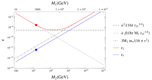
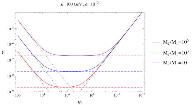
The full CP𝐶𝑃CP asymmetry is obtained by combining the above results for ϵivsuperscriptsubscriptitalic-ϵ𝑖𝑣\epsilon_{i}^{v} (19) and ϵiwsuperscriptsubscriptitalic-ϵ𝑖𝑤\epsilon_{i}^{w} (23). For the hierarchical N1N2subscript𝑁1subscript𝑁2N_{1}-N_{2} regime, with M2/M110subscript𝑀2subscript𝑀110M_{2}/M_{1}\geq 10 that will be of interest later, the CP𝐶𝑃CP-asymmetry can be approximated by the following simple expressions (see Appendix A for details),

ϵ13M1αmα8πv2,ϵ23M2αmα16πv2+(βM2+|α11|2(1σ2))|α21|8πM1M2(1σ2).formulae-sequencesimilar-tosubscriptitalic-ϵ13subscript𝑀1subscript𝛼subscript𝑚𝛼8𝜋superscript𝑣2similar-tosubscriptitalic-ϵ23subscript𝑀2subscript𝛼subscript𝑚𝛼16𝜋superscript𝑣2𝛽subscript𝑀2subscript𝛼1121subscript𝜎2subscript𝛼218𝜋subscript𝑀1subscript𝑀21subscript𝜎2\begin{split}&\epsilon_{1}\sim\frac{3M_{1}\sum_{\alpha}m_{\alpha}}{8\pi v^{2}},\\ &\epsilon_{2}\sim\frac{3M_{2}\sum_{\alpha}m_{\alpha}}{16\pi v^{2}}+\left(\frac{\beta}{M_{2}}+\frac{|\alpha_{11}|}{2}(1-\sigma_{2})\right)\frac{|\alpha_{21}|}{8\pi}\sqrt{\frac{M_{1}}{M_{2}}}(1-\sigma_{2}).\end{split} (25)

The index α=1,2,3𝛼123\alpha=1,2,3, and mαsubscript𝑚𝛼m_{\alpha} is the mass of the α𝛼\alpha-th active neutrino. Assuming a normal hierarchy among the light neutrino masses, we set αmαm3Δm3120.05similar-to-or-equalssubscript𝛼subscript𝑚𝛼subscript𝑚3similar-to-or-equalsΔsuperscriptsubscript𝑚312similar-to0.05\sum_{\alpha}m_{\alpha}\simeq m_{3}\simeq\sqrt{\Delta m_{31}^{2}}\sim 0.05eV.

3 Two-stage Boltzmann evolution

In minimal leptogenesis, the RHN sector λijNjLiH+MiNiNisubscript𝜆𝑖𝑗subscript𝑁𝑗subscript𝐿𝑖𝐻subscript𝑀𝑖subscript𝑁𝑖subscript𝑁𝑖\lambda_{ij}N_{j}L_{i}H+M_{i}N_{i}N_{i} provides the ingredients for two of Sakharov’s conditions to be satisfied; L𝐿L is violated due to the presence of both Misubscript𝑀𝑖M_{i} and λijsubscript𝜆𝑖𝑗\lambda_{ij}, while there are physical CP𝐶𝑃CP-odd phases in λijsubscript𝜆𝑖𝑗\lambda_{ij}. The third and final condition is satisfied dynamically as the expansion of the universe provides a mechanism for L𝐿L-violating processes to go out of equilibrium. For this to happen, the rate ΓNsubscriptΓ𝑁\Gamma_{N} of L𝐿L-violating RHN decays must fall below the Hubble expansion rate H𝐻H. This transition is controlled by the Gamow equilibrium parameter, K=ΓN/H(T=M)𝐾subscriptΓ𝑁𝐻𝑇𝑀K=\Gamma_{N}/H(T=M) Kolb and Turner (1990),222We will follow the literature and denote the Hubble-normalized N𝑁N decay rate as K𝐾K, while the modified Bessel function that generically appears in the thermal rates will consistently be written as Ki(z)subscript𝐾𝑖𝑧K_{i}(z), distinguished by the extra argument z=M/T𝑧𝑀𝑇z=M/T. where the Hubble rate H(T=M)𝐻𝑇𝑀H(T=M) sets the time scale, tHsubscript𝑡𝐻t_{H}, at which the equilibrium density becomes Boltzmann suppressed. Setting K<1𝐾1K<1 ensures the particle lifetime is longer than the Hubble time, τN>tHsubscript𝜏𝑁subscript𝑡𝐻\tau_{N}>t_{H}, and an excess abundance develops. In that case, the rate of decays will be large compared to that of inverse decays in order for the neutrino abundance to be able to reach equilibrium, effectively putting the system out of equilibrium.

In Higgs Portal Leptogenesis, we require at least two Majorana neutrinos and there are two major implications. On one hand, the CP𝐶𝑃CP-asymmetry from N2subscript𝑁2N_{2} decays (25) is enhanced for low masses, and can in fact become the dominant contribution. This suggests the possibility of establishing a ‘lower energy’ theory of leptogenesis, mainly controlled by N2subscript𝑁2N_{2} physics. On the other hand, the two RHN flavors leads to a novel evolution in the total lepton asymmetry. In minimal leptogenesis, the lepton asymmetry is primarily generated in a temperature range near the lightest RHN mass, TM1similar-to𝑇subscript𝑀1T\sim M_{1}, since the decays and scattering are out-of-equilibrium for lower temperatures. The difference here is that, even though most of the lepton asymmetry can be generated through N2subscript𝑁2N_{2} decays and inverse decays at temperatures around TM2similar-to𝑇subscript𝑀2T\sim M_{2}, the lighter neutrino flavor N1subscript𝑁1N_{1} potentially remains in equilibrium and can mediate rapid washout of the N2subscript𝑁2N_{2}-generated asymmetry. These interactions will be studied carefully below, to identify regimes in which N1subscript𝑁1N_{1} is sufficiently weakly coupled that these new washout processes are suppressed.

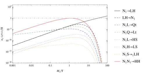
3.1 Boltzmann equations

In the minimal leptogenesis scenario, typically once the neutrino decays go out-of-equilibrium, all the scattering processes also go out-of-equilibrium. The new feature in HPL is the possibility of having scattering processes in equilibrium during the period that a CP𝐶𝑃CP-asymmetry would be generated through out of equilibrium decays. The most significant are those L𝐿L-violating scattering processes with an external N1subscript𝑁1N_{1}, whose abundance is not Boltzmann suppressed. The scattering processes that have an external N2subscript𝑁2N_{2} are of course suppressed by the N2subscript𝑁2N_{2} abundance which rapidly falls off exponentially. Among the scattering processes that violate the lepton number by ΔL=1Δ𝐿1\Delta L=1 units, we include the scattering NiLQt¯subscript𝑁𝑖𝐿𝑄¯𝑡N_{i}L\leftrightarrow Q\overline{t} in the s𝑠s-channel, and NiQLtsubscript𝑁𝑖𝑄𝐿𝑡N_{i}Q\leftrightarrow Lt, NtLQ𝑁𝑡𝐿𝑄Nt\leftrightarrow LQ in the t𝑡t-channel. From the hidden sector, one includes the s𝑠s-channel processes NiLHSsubscript𝑁𝑖𝐿𝐻𝑆N_{i}L\leftrightarrow HS mediated by a Higgs, and NiSLHsubscript𝑁𝑖𝑆𝐿𝐻N_{i}S\leftrightarrow LH mediated by a neutrino. In the t𝑡t-channel one has NiSLHsubscript𝑁𝑖𝑆𝐿𝐻N_{i}S\leftrightarrow LH and NiHLSsubscript𝑁𝑖𝐻𝐿𝑆N_{i}H\leftrightarrow LS both mediated by a Higgs. A full treatment of neutrino-mediated scattering is complicated because of the λijsubscript𝜆𝑖𝑗\lambda_{ij} and αijsubscript𝛼𝑖𝑗\alpha_{ij} flavor structures. For simplicity, we will ignore the flavor-mixing in these processes with intermediate neutrinos, e.g. σNiSLH=jσNiS𝑗LHsubscript𝜎subscript𝑁𝑖𝑆𝐿𝐻subscript𝑗subscript𝜎𝑗absentsubscript𝑁𝑖𝑆𝐿𝐻\sigma_{N_{i}S\leftrightarrow LH}=\sum_{j}\sigma_{N_{i}S\xleftrightarrow[j]{}LH}, and assume the processes are dominated by one flavor. This is sufficient for order of magnitude estimates. Note that because of the αijsubscript𝛼𝑖𝑗\alpha_{ij} coupling, we need to include interactions such as NiNjHHsubscript𝑁𝑖subscript𝑁𝑗𝐻𝐻N_{i}N_{j}\leftrightarrow HH mediated by S𝑆S in the s𝑠s-channel, which can efficiently deplete the neutrino abundance, and in turn affect the lepton asymmetry washout Aristizabal Sierra et al. (2014).333In the context of standard leptogenesis, ΔN=2Δ𝑁2\Delta N=2 interactions, e.g. N1N1HHsubscript𝑁1subscript𝑁1𝐻𝐻N_{1}N_{1}\rightarrow HH mediated by a lepton in the t𝑡t-channel, are negligible since they scale as λ4superscript𝜆4\lambda^{4} which is suppressed for M11015less-than-or-similar-tosubscript𝑀1superscript1015M_{1}\lesssim 10^{15}GeV. Interactions in the ΔN=2Δ𝑁2\Delta N=2 class have for instance been taken into account in the context of GUT theories in Plumacher (1997).

As for the ΔL=2Δ𝐿2\Delta L=2 interactions, one has LHLH¯𝐿𝐻¯𝐿𝐻LH\leftrightarrow\overline{LH} mediated by a neutrino in the s𝑠s-channel, and LLHH𝐿𝐿𝐻𝐻LL\leftrightarrow HH, LL¯HH¯𝐿𝐿𝐻𝐻\overline{LL}\leftrightarrow HH mediated by a neutrino in the t𝑡t-channel. We start by describing the Boltzmann equations for the lepton asymmetry, which are the most complex, and then review the neutrino abundance and the general features. Further technical details are contained in Appendices B and C. Note that this work is concerned with the main dynamical features of the model presented above, focussing on the impact of the Higgs portal couplings. Thus, in deriving the Boltzmann equations, we study only the total lepton asymmetry, ignoring the often significant effects on individual lepton flavors Barbieri et al. (2000); *Abada:2006fw; *Nardi:2006fx; *Endoh:2003mz; *Pilaftsis:2004xx; *Dev:2014laa. For our purposes, it will also be sufficient to utilize the CP𝐶𝑃CP-asymmetries calculated within zero-temperature field theory, although real-time thermal field theory provides a more complete formalism, see e.g. Kiessig and Plumacher (2012a); *Garbrecht:2013iga; *Pilaftsis:2013xna; *Beneke:2010dz; *Kiessig:2011ga; *Frossard:2012pc; *Kiessig:2010pr.

Lepton asymmetry

Starting with the lepton asymmetry equation, we have

nγeqz1HYLL¯z1=i[YiYieq(γNiLHeqγNiLH¯eq)YLYLeqγLHNieq+YL¯YLeqγLH¯NieqYLL¯YLeq(YiYieqγNiLQteq+YiYieqγNiLHSeq+2γNiQLteq+2γNiHLSeq)]YLL¯YLeq(γN1S1LHeq+γN2S1LHeq+γN2S2LHeq)+Y1Y1eq(γN1S2LHeq,subγN1S2LH¯eq,sub)YLYLeqγLH2N1Seq,sub+YL¯YLeqγLH¯2N1Seq,sub2YLYLeqjγLH𝑗LH¯eq,sub+2YL¯YL¯eqjγLH¯𝑗LHeq,sub2YLL¯YLeqjγLL𝑗HHeq.superscriptsubscript𝑛𝛾𝑒𝑞subscript𝑧1𝐻subscript𝑌𝐿¯𝐿subscript𝑧1subscript𝑖delimited-[]subscript𝑌𝑖subscriptsuperscript𝑌𝑒𝑞𝑖subscriptsuperscript𝛾𝑒𝑞subscript𝑁𝑖𝐿𝐻subscriptsuperscript𝛾𝑒𝑞subscript𝑁𝑖¯𝐿𝐻subscript𝑌𝐿subscriptsuperscript𝑌𝑒𝑞𝐿subscriptsuperscript𝛾𝑒𝑞𝐿𝐻subscript𝑁𝑖subscript𝑌¯𝐿subscriptsuperscript𝑌𝑒𝑞𝐿subscriptsuperscript𝛾𝑒𝑞¯𝐿𝐻subscript𝑁𝑖subscript𝑌𝐿¯𝐿subscriptsuperscript𝑌𝑒𝑞𝐿subscript𝑌𝑖subscriptsuperscript𝑌𝑒𝑞𝑖subscriptsuperscript𝛾𝑒𝑞subscript𝑁𝑖𝐿𝑄𝑡subscript𝑌𝑖subscriptsuperscript𝑌𝑒𝑞𝑖subscriptsuperscript𝛾𝑒𝑞subscript𝑁𝑖𝐿𝐻𝑆2subscriptsuperscript𝛾𝑒𝑞subscript𝑁𝑖𝑄𝐿𝑡2subscriptsuperscript𝛾𝑒𝑞subscript𝑁𝑖𝐻𝐿𝑆subscript𝑌𝐿¯𝐿subscriptsuperscript𝑌𝑒𝑞𝐿subscriptsuperscript𝛾𝑒𝑞1absentsubscript𝑁1𝑆𝐿𝐻subscriptsuperscript𝛾𝑒𝑞1absentsubscript𝑁2𝑆𝐿𝐻subscriptsuperscript𝛾𝑒𝑞2absentsubscript𝑁2𝑆𝐿𝐻subscript𝑌1subscriptsuperscript𝑌𝑒𝑞1subscriptsuperscript𝛾𝑒𝑞𝑠𝑢𝑏2absentsubscript𝑁1𝑆𝐿𝐻subscriptsuperscript𝛾𝑒𝑞𝑠𝑢𝑏2absentsubscript𝑁1𝑆¯𝐿𝐻subscript𝑌𝐿subscriptsuperscript𝑌𝑒𝑞𝐿subscriptsuperscript𝛾𝑒𝑞𝑠𝑢𝑏2absent𝐿𝐻subscript𝑁1𝑆subscript𝑌¯𝐿subscriptsuperscript𝑌𝑒𝑞𝐿subscriptsuperscript𝛾𝑒𝑞𝑠𝑢𝑏2absent¯𝐿𝐻subscript𝑁1𝑆2subscript𝑌𝐿subscriptsuperscript𝑌𝑒𝑞𝐿subscript𝑗subscriptsuperscript𝛾𝑒𝑞𝑠𝑢𝑏𝑗absent𝐿𝐻¯𝐿𝐻2subscript𝑌¯𝐿subscriptsuperscript𝑌𝑒𝑞¯𝐿subscript𝑗subscriptsuperscript𝛾𝑒𝑞𝑠𝑢𝑏𝑗absent¯𝐿𝐻𝐿𝐻2subscript𝑌𝐿¯𝐿subscriptsuperscript𝑌𝑒𝑞𝐿subscript𝑗subscriptsuperscript𝛾𝑒𝑞𝑗absent𝐿𝐿𝐻𝐻\begin{split}n_{\gamma}^{eq}z_{1}H\frac{\partial Y_{L-\overline{L}}}{\partial z_{1}}=\sum_{i}\Bigg{[}&\frac{Y_{i}}{Y^{eq}_{i}}\left(\gamma^{eq}_{N_{i}\rightarrow LH}-\gamma^{eq}_{N_{i}\rightarrow\overline{LH}}\right)-\frac{Y_{L}}{Y^{eq}_{L}}\gamma^{eq}_{LH\rightarrow N_{i}}+\frac{Y_{\overline{L}}}{Y^{eq}_{L}}\gamma^{eq}_{\overline{LH}\rightarrow N_{i}}\\ &-\frac{Y_{L-\overline{L}}}{Y^{eq}_{L}}\left(\frac{Y_{i}}{Y^{eq}_{i}}\gamma^{eq}_{N_{i}L\rightarrow Qt}+\frac{Y_{i}}{Y^{eq}_{i}}\gamma^{eq}_{N_{i}L\rightarrow HS}+2\gamma^{eq}_{N_{i}Q\rightarrow Lt}+2\gamma^{eq}_{N_{i}H\rightarrow LS}\right)\Bigg{]}\\ &-\frac{Y_{L-\overline{L}}}{Y^{eq}_{L}}\left(\gamma^{eq}_{N_{1}S\xrightarrow[1]{}LH}+\gamma^{eq}_{N_{2}S\xrightarrow[1]{}LH}+\gamma^{eq}_{N_{2}S\xrightarrow[2]{}LH}\right)\\ &+\frac{Y_{1}}{Y^{eq}_{1}}\left(\gamma^{eq,sub}_{N_{1}S\xrightarrow[2]{}LH}-\gamma^{eq,sub}_{N_{1}S\xrightarrow[2]{}\overline{LH}}\right)-\frac{Y_{L}}{Y^{eq}_{L}}\gamma^{eq,sub}_{LH\xrightarrow[2]{}N_{1}S}+\frac{Y_{\overline{L}}}{Y^{eq}_{L}}\gamma^{eq,sub}_{\overline{LH}\xrightarrow[2]{}N_{1}S}\\ &-2\frac{Y_{L}}{Y^{eq}_{L}}\sum_{j}\gamma^{eq,sub}_{LH\xrightarrow[j]{}\overline{LH}}+2\frac{Y_{\overline{L}}}{Y^{eq}_{\overline{L}}}\sum_{j}\gamma^{eq,sub}_{\overline{LH}\xrightarrow[j]{}LH}\\ &-2\frac{Y_{L-\overline{L}}}{Y^{eq}_{L}}\sum_{j}\gamma^{eq}_{LL\xrightarrow[j]{}HH}.\end{split} (26)

In this expression, we use the following notation,

zi=MiT,Yi=ninγeq,Yieq=38zi2K2(zi),formulae-sequencesubscript𝑧𝑖subscript𝑀𝑖𝑇formulae-sequencesubscript𝑌𝑖subscript𝑛𝑖subscriptsuperscript𝑛𝑒𝑞𝛾subscriptsuperscript𝑌𝑒𝑞𝑖38superscriptsubscript𝑧𝑖2subscript𝐾2subscript𝑧𝑖z_{i}=\frac{M_{i}}{T},\qquad Y_{i}=\frac{n_{i}}{n^{eq}_{\gamma}},\qquad Y^{eq}_{i}=\frac{3}{8}z_{i}^{2}K_{2}(z_{i}), (27)

where Ki(z)subscript𝐾𝑖𝑧K_{i}(z) is a modified Bessel function of the second kind, along with the thermal cross sections,

γimneq(T)=nieqΓimnMiE=nieqK1(zi)K2(zi)Γimn,γijmneq(T)=nieqnjeqvσijmn=gigjT432π4wmin𝑑wwK1(w)σ^ijmn(wmi2zi2),formulae-sequencesubscriptsuperscript𝛾𝑒𝑞𝑖𝑚𝑛𝑇subscriptsuperscript𝑛𝑒𝑞𝑖subscriptΓ𝑖𝑚𝑛delimited-⟨⟩subscript𝑀𝑖𝐸superscriptsubscript𝑛𝑖𝑒𝑞subscript𝐾1subscript𝑧𝑖subscript𝐾2subscript𝑧𝑖subscriptΓ𝑖𝑚𝑛subscriptsuperscript𝛾𝑒𝑞𝑖𝑗𝑚𝑛𝑇subscriptsuperscript𝑛𝑒𝑞𝑖subscriptsuperscript𝑛𝑒𝑞𝑗delimited-⟨⟩𝑣subscript𝜎𝑖𝑗𝑚𝑛subscript𝑔𝑖subscript𝑔𝑗superscript𝑇432superscript𝜋4superscriptsubscriptsubscript𝑤𝑚𝑖𝑛differential-d𝑤𝑤subscript𝐾1𝑤subscript^𝜎𝑖𝑗𝑚𝑛𝑤superscriptsubscript𝑚𝑖2superscriptsubscript𝑧𝑖2\begin{split}&\gamma^{eq}_{i\rightarrow mn}(T)=n^{eq}_{i}\Gamma_{i\rightarrow mn}\left\langle\frac{M_{i}}{E}\right\rangle=n_{i}^{eq}\frac{K_{1}(z_{i})}{K_{2}(z_{i})}\Gamma_{i\rightarrow mn},\\ &\gamma^{eq}_{ij\rightarrow mn}(T)=n^{eq}_{i}n^{eq}_{j}\langle v\sigma_{ij\rightarrow mn\cdots}\rangle=g_{i}g_{j}\frac{T^{4}}{32\pi^{4}}\int_{w_{min}}^{\infty}dw\sqrt{w}K_{1}\left(\sqrt{w}\right)\hat{\sigma}_{ij\rightarrow mn}\left(w\frac{m_{i}^{2}}{z_{i}^{2}}\right),\end{split} (28)

where w=s/T2𝑤𝑠superscript𝑇2w=s/T^{2}, and the reduced cross section σ^^𝜎\hat{\sigma} is given by

σ^ijmn(s)=1sδ(s,mi2,mj2)σijmn(s),δ(a,b,c)=(abc)24bc.formulae-sequencesubscript^𝜎𝑖𝑗𝑚𝑛𝑠1𝑠𝛿𝑠superscriptsubscript𝑚𝑖2superscriptsubscript𝑚𝑗2subscript𝜎𝑖𝑗𝑚𝑛𝑠𝛿𝑎𝑏𝑐superscript𝑎𝑏𝑐24𝑏𝑐\hat{\sigma}_{ij\rightarrow mn}(s)=\frac{1}{s}\delta\left(s,m_{i}^{2},m_{j}^{2}\right)\sigma_{ij\rightarrow mn}(s),\qquad\delta(a,b,c)=(a-b-c)^{2}-4bc. (29)

In Appendix B, we include further details about the Boltzmann equations and thermal cross sections. In writing the above equation, we have assumed CP𝐶𝑃CP-invariance, γij¯mn¯eq=γijmneqsubscriptsuperscript𝛾𝑒𝑞¯𝑖𝑗¯𝑚𝑛subscriptsuperscript𝛾𝑒𝑞𝑖𝑗𝑚𝑛\gamma^{eq}_{\overline{ij}\rightarrow\overline{mn}}=\gamma^{eq}_{ij\rightarrow mn} in the scattering processes, along with CPT𝐶𝑃𝑇CPT-symmetry, γij¯mn¯eq=γmnijeqsubscriptsuperscript𝛾𝑒𝑞¯𝑖𝑗¯𝑚𝑛subscriptsuperscript𝛾𝑒𝑞𝑚𝑛𝑖𝑗\gamma^{eq}_{\overline{ij}\rightarrow\overline{mn}}=\gamma^{eq}_{mn\rightarrow ij}. CP𝐶𝑃CP-violating corrections appear in the scattering amplitudes at fourth order in the coupling constants, which is of higher order than we will consider here. That being said, it is necessary to make an exception when dealing with the subtracted rates as discussed below.

The superscript ‘sub𝑠𝑢𝑏sub’ signifies that the process contains a real-intermediate-state (RIS) mediator that should be subtracted. Most famously, the process LHLH¯𝐿𝐻¯𝐿𝐻LH\rightarrow\overline{LH} is mediated by a neutrino Njsubscript𝑁𝑗N_{j} in the s𝑠s-channel which can be on-shell for a sufficiently high center of mass energy. The real intermediate state represents the physical process LHNjLH¯𝐿𝐻subscript𝑁𝑗¯𝐿𝐻LH\rightarrow N_{j}\rightarrow\overline{LH}. However, these processes are already accounted for by decays and inverse decays, and therefore need to be removed. Similarly, N1S2LH2absentsubscript𝑁1𝑆𝐿𝐻N_{1}S\xrightarrow[2]{}LH has the real intermediate state N1SN2LHsubscript𝑁1𝑆subscript𝑁2𝐿𝐻N_{1}S\rightarrow N_{2}\rightarrow LH, which is also accounted for by decays and inverse decays. As it turns out, the t𝑡t-channel process NiHLSsubscript𝑁𝑖𝐻𝐿𝑆N_{i}H\rightarrow LS also contains a real intermediate state, that needs to be removed. This point is explained in Appendix C, where explicit formulas for the cross sections are displayed. For simplicity, all quarks and leptons, as well as the Higgs and scalar S𝑆S are considered massless. This can be justified because leptogenesis necessarily occurs at temperatures above sphaleron decoupling, T>Tsphaleron160GeV>mH𝑇subscript𝑇𝑠𝑝𝑎𝑙𝑒𝑟𝑜𝑛similar-to160GeVsubscript𝑚𝐻T>T_{sphaleron}\sim 160\,\text{GeV}>m_{H} D’Onofrio et al. (2014), though typically we shall take M2>1subscript𝑀21M_{2}>1~{}TeV. The singlet S𝑆S mass is not yet stringently constrained, provided the Higgs portal coupling is not too large Aad et al. (2014), but we will typically take it to be of the same order as the Higgs mass. With these simplifications, the t𝑡t-channel processes NiQLtsubscript𝑁𝑖𝑄𝐿𝑡N_{i}Q\leftrightarrow Lt and NitLQsubscript𝑁𝑖𝑡𝐿𝑄N_{i}t\rightarrow LQ have equal rates, and similarly for NiHLSsubscript𝑁𝑖𝐻𝐿𝑆N_{i}H\rightarrow LS and NiSLHsubscript𝑁𝑖𝑆𝐿𝐻N_{i}S\rightarrow LH, which explains the factor of ‘2’ sitting in front of these processes in Eq. (26) above.

Subtracted Rates and Real Intermediate States

Refer to caption

Figure 5: Classes of decay and scattering diagrams and sub-diagrams. We subtract the Nisubscript𝑁𝑖N_{i} real intermediate states coupling through α𝛼\alpha and λ𝜆\lambda order by order to avoid double counting, as discussed in the text.

In this subsection, we summarize the procedure used to account for real intermediate states. The source terms in the Boltzmann equations are systematically expanded in each of the couplings and one needs to avoid double counting the RIS contributions that appear in (naively) higher order scattering processes. Doing this consistently in standard leptogenesis requires the inclusion of all processes up to and including two-to-three scattering and the associated CP𝐶𝑃CP-asymmetries Abada et al. (2006b); *Nardi:2007jp. For HPL, we will do the same, extending the analysis to account for real intermediate states coupling via both the Yukawa λijsubscript𝜆𝑖𝑗\lambda_{ij} and the singlet αijsubscript𝛼𝑖𝑗\alpha_{ij} interactions. The relevant tree-level diagrams are displayed in Fig. 5, although it’s important to account also for loop corrections that contribute to the CP𝐶𝑃CP-asymmetries in scattering. As already mentioned, we will focus on the impact of the additional singlet decay channel and ignore the issue of neutrino flavor mixing in scattering amplitudes, e.g. γLHLH¯eq=iγLH𝑖LH¯eqsubscriptsuperscript𝛾𝑒𝑞𝐿𝐻¯𝐿𝐻subscript𝑖subscriptsuperscript𝛾𝑒𝑞𝑖absent𝐿𝐻¯𝐿𝐻\gamma^{eq}_{LH\rightarrow\overline{LH}}=\sum_{i}\gamma^{eq}_{LH\xrightarrow[i]{}\overline{LH}}, which has been discussed in detail elsewhere. The RIS calculation of the s𝑠s-channel cross sections is generally a nontrivial task once the flavor structure is taken into account. However, given this simplifying assumption, we can use the result γsub=γγonshellsuperscript𝛾𝑠𝑢𝑏𝛾superscript𝛾𝑜𝑛𝑠𝑒𝑙𝑙\gamma^{sub}=\gamma-\gamma^{on-shell} Kolb and Wolfram (1980); *Strumia:2006qk.

To proceed to discuss the subtracted rates, we first make the following definitions associated with N2subscript𝑁2N_{2} decays,

Γ2T=Γ2+ΓN2N1S,Γ2=ΓN2LH+ΓN2LH¯,ϵ2Γ2=ΓN2LHΓN2LH¯,Br(N2LH)=1+ϵ22Γ2Γ2T,Br(N2LH¯)=1ϵ22Γ2Γ2T,Br(N2N1S)=Γ21Γ2T=1Γ2Γ2T,formulae-sequencesubscriptΓ2𝑇subscriptΓ2subscriptΓsubscript𝑁2subscript𝑁1𝑆formulae-sequencesubscriptΓ2subscriptΓsubscript𝑁2𝐿𝐻subscriptΓsubscript𝑁2¯𝐿𝐻subscriptitalic-ϵ2subscriptΓ2subscriptΓsubscript𝑁2𝐿𝐻subscriptΓsubscript𝑁2¯𝐿𝐻formulae-sequenceBrsubscript𝑁2𝐿𝐻1subscriptitalic-ϵ22subscriptΓ2subscriptΓ2𝑇formulae-sequenceBrsubscript𝑁2¯𝐿𝐻1subscriptitalic-ϵ22subscriptΓ2subscriptΓ2𝑇Brsubscript𝑁2subscript𝑁1𝑆subscriptΓ21subscriptΓ2𝑇1subscriptΓ2subscriptΓ2𝑇\begin{split}&\Gamma_{2T}=\Gamma_{2}+\Gamma_{N_{2}\rightarrow N_{1}S},\\ &\Gamma_{2}=\Gamma_{N_{2}\rightarrow LH}+\Gamma_{N_{2}\rightarrow\overline{LH}},\\ &\epsilon_{2}\Gamma_{2}=\Gamma_{N_{2}\rightarrow LH}-\Gamma_{N_{2}\rightarrow\overline{LH}},\end{split}\quad\Longrightarrow\quad\begin{split}&\text{Br}(N_{2}\rightarrow LH)=\frac{1+\epsilon_{2}}{2}\frac{\Gamma_{2}}{\Gamma_{2T}},\\ &\text{Br}(N_{2}\rightarrow\overline{LH})=\frac{1-\epsilon_{2}}{2}\frac{\Gamma_{2}}{\Gamma_{2T}},\\ &\text{Br}(N_{2}\rightarrow N_{1}S)=\frac{\Gamma_{21}}{\Gamma_{2T}}=1-\frac{\Gamma_{2}}{\Gamma_{2T}},\end{split} (30)

where Γ21subscriptΓ21\Gamma_{21} is shorthand notation for ΓN2N1SsubscriptΓsubscript𝑁2subscript𝑁1𝑆\Gamma_{N_{2}\rightarrow N_{1}S}, while N1subscript𝑁1N_{1} only decays to leptons, so that

Γ1T=Γ1,Γ1=ΓN1LH+ΓN1LH¯,ϵ1Γ1=ΓN1LHΓN1LH¯,Br(N1LH)=1+ϵ12,Br(N1LH¯)=1ϵ12.formulae-sequencesubscriptΓ1𝑇subscriptΓ1formulae-sequencesubscriptΓ1subscriptΓsubscript𝑁1𝐿𝐻subscriptΓsubscript𝑁1¯𝐿𝐻subscriptitalic-ϵ1subscriptΓ1subscriptΓsubscript𝑁1𝐿𝐻subscriptΓsubscript𝑁1¯𝐿𝐻formulae-sequenceBrsubscript𝑁1𝐿𝐻1subscriptitalic-ϵ12Brsubscript𝑁1¯𝐿𝐻1subscriptitalic-ϵ12\begin{split}&\Gamma_{1T}=\Gamma_{1},\\ &\Gamma_{1}=\Gamma_{N_{1}\rightarrow LH}+\Gamma_{N_{1}\rightarrow\overline{LH}},\\ &\epsilon_{1}\Gamma_{1}=\Gamma_{N_{1}\rightarrow LH}-\Gamma_{N_{1}\rightarrow\overline{LH}},\end{split}\quad\Longrightarrow\quad\begin{split}&\text{Br}(N_{1}\rightarrow LH)=\frac{1+\epsilon_{1}}{2},\\ &\text{Br}(N_{1}\rightarrow\overline{LH})=\frac{1-\epsilon_{1}}{2}.\end{split} (31)
Refer to caption
Refer to caption
Refer to caption
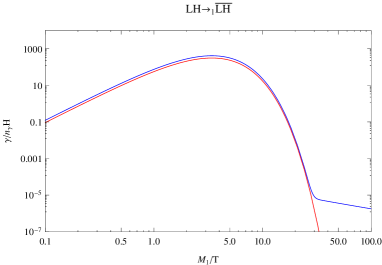
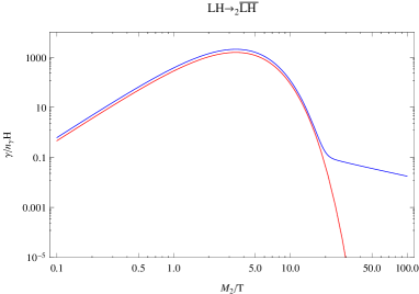
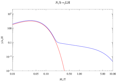
Figure 6: Plots of the un-subtracted thermal rates (blue), along with their on-shell parts (red). The plots in (a), (b) and (c) are for LH1LH¯1absent𝐿𝐻¯𝐿𝐻LH\xrightarrow[1]{}\overline{LH}, LH2LH¯2absent𝐿𝐻¯𝐿𝐻LH\xrightarrow[2]{}\overline{LH}, and N1S2LH2absentsubscript𝑁1𝑆𝐿𝐻N_{1}S\xrightarrow[2]{}LH respectively, generated using λ10.002similar-tosubscript𝜆10.002\lambda_{1}\sim 0.002, λ20.07similar-tosubscript𝜆20.07\lambda_{2}\sim 0.07, α120.07similar-tosubscript𝛼120.07\alpha_{12}\sim 0.07, M2=1010subscript𝑀2superscript1010M_{2}=10^{10}GeV, M1=108subscript𝑀1superscript108M_{1}=10^{8}GeV.

Building up the equations order by order, we have the following contributions:

  • 𝒪(λ2)𝒪superscript𝜆2\mathcal{O}(\lambda^{2}): 1-to-2 decays,

    nγeqz1HYLL¯z1|λ2=i=1,2[YiYieq(γNiLHeqγNiLH¯eq)YLYLeqγLHNieq+YL¯YLeqγLH¯Nieq]=(Y1Y1eq+1)ϵ1γD1eq+(Y2Y2eq+1)ϵ2γD2eqYLL¯2YLeq(γD1eq+γD2eq).evaluated-atsuperscriptsubscript𝑛𝛾𝑒𝑞subscript𝑧1𝐻subscript𝑌𝐿¯𝐿subscript𝑧1superscript𝜆2subscript𝑖12delimited-[]subscript𝑌𝑖subscriptsuperscript𝑌𝑒𝑞𝑖subscriptsuperscript𝛾𝑒𝑞subscript𝑁𝑖𝐿𝐻subscriptsuperscript𝛾𝑒𝑞subscript𝑁𝑖¯𝐿𝐻subscript𝑌𝐿subscriptsuperscript𝑌𝑒𝑞𝐿subscriptsuperscript𝛾𝑒𝑞𝐿𝐻subscript𝑁𝑖subscript𝑌¯𝐿subscriptsuperscript𝑌𝑒𝑞𝐿subscriptsuperscript𝛾𝑒𝑞¯𝐿𝐻subscript𝑁𝑖subscript𝑌1subscriptsuperscript𝑌𝑒𝑞11subscriptitalic-ϵ1superscriptsubscript𝛾subscript𝐷1𝑒𝑞subscript𝑌2subscriptsuperscript𝑌𝑒𝑞21subscriptitalic-ϵ2superscriptsubscript𝛾subscript𝐷2𝑒𝑞subscript𝑌𝐿¯𝐿2subscriptsuperscript𝑌𝑒𝑞𝐿subscriptsuperscript𝛾𝑒𝑞subscript𝐷1subscriptsuperscript𝛾𝑒𝑞subscript𝐷2\begin{split}n_{\gamma}^{eq}z_{1}H\frac{\partial Y_{L-\overline{L}}}{\partial z_{1}}\Bigg{|}_{\lambda^{2}}=&\sum_{i=1,2}\Bigg{[}\frac{Y_{i}}{Y^{eq}_{i}}\left(\gamma^{eq}_{N_{i}\rightarrow LH}-\gamma^{eq}_{N_{i}\rightarrow\overline{LH}}\right)-\frac{Y_{L}}{Y^{eq}_{L}}\gamma^{eq}_{LH\rightarrow N_{i}}+\frac{Y_{\overline{L}}}{Y^{eq}_{L}}\gamma^{eq}_{\overline{LH}\rightarrow N_{i}}\Bigg{]}\\ =&\left(\frac{Y_{1}}{Y^{eq}_{1}}+1\right)\epsilon_{1}\gamma_{D_{1}}^{eq}+\left(\frac{Y_{2}}{Y^{eq}_{2}}+1\right)\epsilon_{2}\gamma_{D_{2}}^{eq}-\frac{Y_{L-\overline{L}}}{2Y^{eq}_{L}}\left(\gamma^{eq}_{D_{1}}+\gamma^{eq}_{D_{2}}\right).\end{split} (32)

    This Boltzmann equation suffers from the well-known flaw that it does not respect Sakharov conditions. Indeed, even in equilibrium Yi=Yieqsubscript𝑌𝑖subscriptsuperscript𝑌𝑒𝑞𝑖Y_{i}=Y^{eq}_{i}, a lepton asymmetry may be generated because of the non-vanishing source term. This is related to the fact that at 𝒪(λ2)𝒪superscript𝜆2\mathcal{O}(\lambda^{2}), the set of interactions is incomplete because ΔL=2Δ𝐿2\Delta L=2 rates at (naive) 𝒪(λ4)𝒪superscript𝜆4\mathcal{O}(\lambda^{4}) contain real intermediate state contributions that are in fact of order 𝒪(λ2)𝒪superscript𝜆2\mathcal{O}(\lambda^{2}) and need to be included; see below.

  • 𝒪(λ4)𝒪superscript𝜆4\mathcal{O}(\lambda^{4}): ΔL=2Δ𝐿2\Delta L=2 scattering (2-to-2),

    nγeqz1HYLL¯z1|λ4=j=1,2[2YLYLeqγLH𝑗LH¯eq,sub+2YL¯YL¯eqγLH¯𝑗LHeq,sub]=2ϵ1γD1eq2ϵ2Γ2Γ2TγD2eqYLL¯YLeq(2γΔL=2eq,sub,2+2γΔL=2eq,sub,1),evaluated-atsuperscriptsubscript𝑛𝛾𝑒𝑞subscript𝑧1𝐻subscript𝑌𝐿¯𝐿subscript𝑧1superscript𝜆4subscript𝑗12delimited-[]2subscript𝑌𝐿subscriptsuperscript𝑌𝑒𝑞𝐿subscriptsuperscript𝛾𝑒𝑞𝑠𝑢𝑏𝑗absent𝐿𝐻¯𝐿𝐻2subscript𝑌¯𝐿subscriptsuperscript𝑌𝑒𝑞¯𝐿subscriptsuperscript𝛾𝑒𝑞𝑠𝑢𝑏𝑗absent¯𝐿𝐻𝐿𝐻2subscriptitalic-ϵ1superscriptsubscript𝛾subscript𝐷1𝑒𝑞2subscriptitalic-ϵ2subscriptΓ2subscriptΓ2𝑇superscriptsubscript𝛾subscript𝐷2𝑒𝑞subscript𝑌𝐿¯𝐿subscriptsuperscript𝑌𝑒𝑞𝐿2subscriptsuperscript𝛾𝑒𝑞𝑠𝑢𝑏2Δ𝐿22subscriptsuperscript𝛾𝑒𝑞𝑠𝑢𝑏1Δ𝐿2\begin{split}n_{\gamma}^{eq}z_{1}H\frac{\partial Y_{L-\overline{L}}}{\partial z_{1}}\Bigg{|}_{\lambda^{4}}=&\sum_{j=1,2}\Bigg{[}-2\frac{Y_{L}}{Y^{eq}_{L}}\gamma^{eq,sub}_{LH\xrightarrow[j]{}\overline{LH}}+2\frac{Y_{\overline{L}}}{Y^{eq}_{\overline{L}}}\gamma^{eq,sub}_{\overline{LH}\xrightarrow[j]{}LH}\Bigg{]}\\ &=-2\epsilon_{1}\gamma_{D_{1}}^{eq}-2\epsilon_{2}\frac{\Gamma_{2}}{\Gamma_{2T}}\gamma_{D_{2}}^{eq}-\frac{Y_{L-\overline{L}}}{Y^{eq}_{L}}\left(2\gamma^{eq,sub,2}_{\Delta L=2}+2\gamma^{eq,sub,1}_{\Delta L=2}\right),\end{split} (33)

    where we used the definitions for the subtracted ΔL=2Δ𝐿2\Delta L=2 rates,

    γLH2LH¯eq,onshell=γLHN2eqBr(N2LH¯)=(1ϵ22)2Γ2Γ2TγD2eq12ϵ24Γ2Γ2TγD2eq,γLH2LH¯eq,sub=γΔL=2eq,sub,(2)ϵ22Γ2Γ2TγD2eq,γΔL=2eq,sub,(2)γLH2LH¯eq14Γ2Γ2TγD2eq,ΔγΔL=2eq,sub,(2)γLH2LH¯eq,subγLH¯2LHeq,sub=ϵ2Γ2Γ2TγD2eq,formulae-sequencesubscriptsuperscript𝛾𝑒𝑞𝑜𝑛𝑠𝑒𝑙𝑙2absent𝐿𝐻¯𝐿𝐻subscriptsuperscript𝛾𝑒𝑞𝐿𝐻subscript𝑁2Brsubscript𝑁2¯𝐿𝐻superscript1subscriptitalic-ϵ222subscriptΓ2subscriptΓ2𝑇subscriptsuperscript𝛾𝑒𝑞subscript𝐷212subscriptitalic-ϵ24subscriptΓ2subscriptΓ2𝑇subscriptsuperscript𝛾𝑒𝑞subscript𝐷2formulae-sequencesubscriptsuperscript𝛾𝑒𝑞𝑠𝑢𝑏2absent𝐿𝐻¯𝐿𝐻subscriptsuperscript𝛾𝑒𝑞𝑠𝑢𝑏2Δ𝐿2subscriptitalic-ϵ22subscriptΓ2subscriptΓ2𝑇subscriptsuperscript𝛾𝑒𝑞subscript𝐷2formulae-sequencesubscriptsuperscript𝛾𝑒𝑞𝑠𝑢𝑏2Δ𝐿2subscriptsuperscript𝛾𝑒𝑞2absent𝐿𝐻¯𝐿𝐻14subscriptΓ2subscriptΓ2𝑇subscriptsuperscript𝛾𝑒𝑞subscript𝐷2Δsubscriptsuperscript𝛾𝑒𝑞𝑠𝑢𝑏2Δ𝐿2subscriptsuperscript𝛾𝑒𝑞𝑠𝑢𝑏2absent𝐿𝐻¯𝐿𝐻subscriptsuperscript𝛾𝑒𝑞𝑠𝑢𝑏2absent¯𝐿𝐻𝐿𝐻subscriptitalic-ϵ2subscriptΓ2subscriptΓ2𝑇subscriptsuperscript𝛾𝑒𝑞subscript𝐷2\begin{split}&\gamma^{eq,on-shell}_{LH\xrightarrow[2]{}\overline{LH}}=\gamma^{eq}_{LH\rightarrow N_{2}}\text{Br}(N_{2}\rightarrow\overline{LH})=\left(\frac{1-\epsilon_{2}}{2}\right)^{2}\frac{\Gamma_{2}}{\Gamma_{2T}}\gamma^{eq}_{D_{2}}\approx\frac{1-2\epsilon_{2}}{4}\frac{\Gamma_{2}}{\Gamma_{2T}}\gamma^{eq}_{D_{2}},\\ &\gamma^{eq,sub}_{LH\xrightarrow[2]{}\overline{LH}}=\gamma^{eq,sub,(2)}_{\Delta L=2}-\frac{\epsilon_{2}}{2}\frac{\Gamma_{2}}{\Gamma_{2T}}\gamma^{eq}_{D_{2}},\\ &\gamma^{eq,sub,(2)}_{\Delta L=2}\equiv\gamma^{eq}_{LH\xrightarrow[2]{}\overline{LH}}-\frac{1}{4}\frac{\Gamma_{2}}{\Gamma_{2T}}\gamma^{eq}_{D_{2}},\\ &\Delta\gamma^{eq,sub,(2)}_{\Delta L=2}\equiv\gamma^{eq,sub}_{LH\xrightarrow[2]{}\overline{LH}}-\gamma^{eq,sub}_{\overline{LH}\xrightarrow[2]{}LH}=-\epsilon_{2}\frac{\Gamma_{2}}{\Gamma_{2T}}\gamma^{eq}_{D_{2}},\end{split} (34)

    and

    γLH1LH¯eq,onshell=γLHN1eqBr(N1LH¯)=(1ϵ12)2γD1eq12ϵ14γD2eq,γLH1LH¯eq,sub=γΔL=2eq,sub,(1)ϵ12γD1eq,γΔL=2eq,sub,(1)γLH1LH¯eq14γD1eq,ΔγΔL=2eq,sub,(1)γLH1LH¯eq,subγLH¯1LHeq,sub=ϵ1γD1eq.formulae-sequencesubscriptsuperscript𝛾𝑒𝑞𝑜𝑛𝑠𝑒𝑙𝑙1absent𝐿𝐻¯𝐿𝐻subscriptsuperscript𝛾𝑒𝑞𝐿𝐻subscript𝑁1Brsubscript𝑁1¯𝐿𝐻superscript1subscriptitalic-ϵ122subscriptsuperscript𝛾𝑒𝑞subscript𝐷112subscriptitalic-ϵ14subscriptsuperscript𝛾𝑒𝑞subscript𝐷2formulae-sequencesubscriptsuperscript𝛾𝑒𝑞𝑠𝑢𝑏1absent𝐿𝐻¯𝐿𝐻subscriptsuperscript𝛾𝑒𝑞𝑠𝑢𝑏1Δ𝐿2subscriptitalic-ϵ12subscriptsuperscript𝛾𝑒𝑞subscript𝐷1formulae-sequencesubscriptsuperscript𝛾𝑒𝑞𝑠𝑢𝑏1Δ𝐿2subscriptsuperscript𝛾𝑒𝑞1absent𝐿𝐻¯𝐿𝐻14subscriptsuperscript𝛾𝑒𝑞subscript𝐷1Δsubscriptsuperscript𝛾𝑒𝑞𝑠𝑢𝑏1Δ𝐿2subscriptsuperscript𝛾𝑒𝑞𝑠𝑢𝑏1absent𝐿𝐻¯𝐿𝐻subscriptsuperscript𝛾𝑒𝑞𝑠𝑢𝑏1absent¯𝐿𝐻𝐿𝐻subscriptitalic-ϵ1subscriptsuperscript𝛾𝑒𝑞subscript𝐷1\begin{split}&\gamma^{eq,on-shell}_{LH\xrightarrow[1]{}\overline{LH}}=\gamma^{eq}_{LH\rightarrow N_{1}}\text{Br}(N_{1}\rightarrow\overline{LH})=\left(\frac{1-\epsilon_{1}}{2}\right)^{2}\gamma^{eq}_{D_{1}}\approx\frac{1-2\epsilon_{1}}{4}\gamma^{eq}_{D_{2}},\\ &\gamma^{eq,sub}_{LH\xrightarrow[1]{}\overline{LH}}=\gamma^{eq,sub,(1)}_{\Delta L=2}-\frac{\epsilon_{1}}{2}\gamma^{eq}_{D_{1}},\\ &\gamma^{eq,sub,(1)}_{\Delta L=2}\equiv\gamma^{eq}_{LH\xrightarrow[1]{}\overline{LH}}-\frac{1}{4}\gamma^{eq}_{D_{1}},\\ &\Delta\gamma^{eq,sub,(1)}_{\Delta L=2}\equiv\gamma^{eq,sub}_{LH\xrightarrow[1]{}\overline{LH}}-\gamma^{eq,sub}_{\overline{LH}\xrightarrow[1]{}LH}=-\epsilon_{1}\gamma^{eq}_{D_{1}}.\end{split} (35)

    The unsubtracted ΔL=2Δ𝐿2\Delta L=2 rates are CP𝐶𝑃CP-symmetric at 𝒪(λ2)𝒪superscript𝜆2\mathcal{O}(\lambda^{2}), which implies that the subtracted rates are in fact CP𝐶𝑃CP-asymmetric. The functions γΔL=2eq,sub,(i)subscriptsuperscript𝛾𝑒𝑞𝑠𝑢𝑏𝑖Δ𝐿2\gamma^{eq,sub,(i)}_{\Delta L=2} are the CP𝐶𝑃CP-conserving parts of the subtracted ΔL=2Δ𝐿2\Delta L=2 rates, and have been plotted in Fig. 6 and 6, showing that the CP𝐶𝑃CP-conserving subtracted rates are negligible.

    Note that the RIS CP𝐶𝑃CP-asymmetry that comes from the N1subscript𝑁1N_{1}-mediated ΔL=2Δ𝐿2\Delta L=2 rate corrects the flaw above in the Boltzmann equation (32). The ΔL=2Δ𝐿2\Delta L=2 rates mediated by N2subscript𝑁2N_{2} however do not fully correct the above Boltzmann equation. This is in contrast to the standard case, the reason being that Br(N2N1S)>0Brsubscript𝑁2subscript𝑁1𝑆0\text{Br}(N_{2}\rightarrow N_{1}S)>0, so there is a second decay channel. Unlike in the standard case, for HPL, obtaining a consistent set of Boltzmann equations requires including the RIS contributions from higher order ΔL=2Δ𝐿2\Delta L=2 scattering processes; see Eq. (36) below.

  • 𝒪(λ4α2)𝒪superscript𝜆4superscript𝛼2\mathcal{O}(\lambda^{4}\alpha^{2}): ΔL=2Δ𝐿2\Delta L=2 scattering (2-to-3),

    nγeqz1HYLL¯z1|λ4α2=4YLYLeqγLH2LH¯Seq,sub+4YL¯YLeqγLH¯2LHSeq,sub=2ϵ2Γ21Γ2TγD2eq4YLL¯YLeqγΔL=2eq,(23)2ΔγΔL=1eq,sub2ϵ1Γ21Γ2TγD2eq,evaluated-atsuperscriptsubscript𝑛𝛾𝑒𝑞subscript𝑧1𝐻subscript𝑌𝐿¯𝐿subscript𝑧1superscript𝜆4superscript𝛼24subscript𝑌𝐿subscriptsuperscript𝑌𝑒𝑞𝐿subscriptsuperscript𝛾𝑒𝑞𝑠𝑢𝑏2absent𝐿𝐻¯𝐿𝐻𝑆4subscript𝑌¯𝐿subscriptsuperscript𝑌𝑒𝑞𝐿subscriptsuperscript𝛾𝑒𝑞𝑠𝑢𝑏2absent¯𝐿𝐻𝐿𝐻𝑆2subscriptitalic-ϵ2subscriptΓ21subscriptΓ2𝑇subscriptsuperscript𝛾𝑒𝑞subscript𝐷24subscript𝑌𝐿¯𝐿subscriptsuperscript𝑌𝑒𝑞𝐿subscriptsuperscript𝛾𝑒𝑞23Δ𝐿22Δsubscriptsuperscript𝛾𝑒𝑞𝑠𝑢𝑏Δ𝐿12subscriptitalic-ϵ1subscriptΓ21subscriptΓ2𝑇subscriptsuperscript𝛾𝑒𝑞subscript𝐷2\begin{split}n_{\gamma}^{eq}z_{1}H\frac{\partial Y_{L-\overline{L}}}{\partial z_{1}}\Bigg{|}_{\lambda^{4}\alpha^{2}}=&-4\frac{Y_{L}}{Y^{eq}_{L}}\gamma^{eq,sub}_{LH\xrightarrow[2]{}\overline{LH}S}+4\frac{Y_{\overline{L}}}{Y^{eq}_{L}}\gamma^{eq,sub}_{\overline{LH}\xrightarrow[2]{}LHS}\\ =&-2\epsilon_{2}\frac{\Gamma_{21}}{\Gamma_{2T}}\gamma^{eq}_{D_{2}}-4\frac{Y_{L-\overline{L}}}{Y^{eq}_{L}}\gamma^{eq,(2-3)}_{\Delta L=2}\\ &-2\Delta\gamma^{eq,sub}_{\Delta L=1}-2\epsilon_{1}\frac{\Gamma_{21}}{\Gamma_{2T}}\gamma^{eq}_{D_{2}},\end{split} (36)

    where we have defined

    γLH2LH¯Seq,onshell=γLH2N1Seq,sub1ϵ12+(1ϵ1)(1ϵ2)4Γ21Γ2TγD2eq,γLH2LH¯Seq,sub=γLH2LH¯SeqγΔL=2eq,(23)+14ΔγΔL=1eq,sub+ϵ1+ϵ24Γ21Γ2TγD2eq,γΔL=2eq,(23)=γLH2LH¯Seq14γΔL=1eq,formulae-sequencesubscriptsuperscript𝛾𝑒𝑞𝑜𝑛𝑠𝑒𝑙𝑙2absent𝐿𝐻¯𝐿𝐻𝑆subscriptsuperscript𝛾𝑒𝑞𝑠𝑢𝑏2absent𝐿𝐻subscript𝑁1𝑆1subscriptitalic-ϵ121subscriptitalic-ϵ11subscriptitalic-ϵ24subscriptΓ21subscriptΓ2𝑇subscriptsuperscript𝛾𝑒𝑞subscript𝐷2formulae-sequencesubscriptsuperscript𝛾𝑒𝑞𝑠𝑢𝑏2absent𝐿𝐻¯𝐿𝐻𝑆subscriptsuperscript𝛾𝑒𝑞2absent𝐿𝐻¯𝐿𝐻𝑆subscriptsuperscript𝛾𝑒𝑞23Δ𝐿214Δsubscriptsuperscript𝛾𝑒𝑞𝑠𝑢𝑏Δ𝐿1subscriptitalic-ϵ1subscriptitalic-ϵ24subscriptΓ21subscriptΓ2𝑇subscriptsuperscript𝛾𝑒𝑞subscript𝐷2subscriptsuperscript𝛾𝑒𝑞23Δ𝐿2subscriptsuperscript𝛾𝑒𝑞2absent𝐿𝐻¯𝐿𝐻𝑆14subscriptsuperscript𝛾𝑒𝑞Δ𝐿1\begin{split}&\gamma^{eq,on-shell}_{LH\xrightarrow[2]{}\overline{LH}S}=\gamma^{eq,sub}_{LH\xrightarrow[2]{}N_{1}S}\frac{1-\epsilon_{1}}{2}+\frac{(1-\epsilon_{1})(1-\epsilon_{2})}{4}\frac{\Gamma_{21}}{\Gamma_{2T}}\gamma^{eq}_{D_{2}},\\ &\gamma^{eq,sub}_{LH\xrightarrow[2]{}\overline{LH}S}=\gamma^{eq}_{LH\xrightarrow[2]{}\overline{LH}S}-\gamma^{eq,(2-3)}_{\Delta L=2}+\frac{1}{4}\Delta\gamma^{eq,sub}_{\Delta L=1}+\frac{\epsilon_{1}+\epsilon_{2}}{4}\frac{\Gamma_{21}}{\Gamma_{2T}}\gamma^{eq}_{D_{2}},\\ &\gamma^{eq,(2-3)}_{\Delta L=2}=\gamma^{eq}_{LH\xrightarrow[2]{}\overline{LH}S}-\frac{1}{4}\gamma^{eq}_{\Delta L=1},\end{split} (37)

    ignoring terms of order 𝒪(λ6α2)𝒪superscript𝜆6superscript𝛼2\mathcal{O}(\lambda^{6}\alpha^{2}) and above. The functions γΔL=1eqsubscriptsuperscript𝛾𝑒𝑞Δ𝐿1\gamma^{eq}_{\Delta L=1} and ΔγΔL=1eq,subΔsubscriptsuperscript𝛾𝑒𝑞𝑠𝑢𝑏Δ𝐿1\Delta\gamma^{eq,sub}_{\Delta L=1} are the CP𝐶𝑃CP-conserving and CP𝐶𝑃CP-violating parts of the N1S2LH2absentsubscript𝑁1𝑆𝐿𝐻N_{1}S\xrightarrow[2]{}LH scattering terms, as is defined in equations (39) below.

    In Eq. (36), the factors of 4 arise on accounting for both LH2LH¯S2absent𝐿𝐻¯𝐿𝐻𝑆LH\xrightarrow[2]{}\overline{LH}S and LHS2LH¯2absent𝐿𝐻𝑆¯𝐿𝐻LHS\xrightarrow[2]{}\overline{LH}, which are CPT𝐶𝑃𝑇CPT conjugates of each other. The first term on the first line is exactly what is needed to combine with the RIS term from Eq. (33) and correct the flaw in (32). The second line of Eq. (36) in fact contains terms that correspond to RIS contributions at 𝒪(λ2α2)𝒪superscript𝜆2superscript𝛼2\mathcal{O}(\lambda^{2}\alpha^{2}).

  • 𝒪(λ2α2)𝒪superscript𝜆2superscript𝛼2\mathcal{O}(\lambda^{2}\alpha^{2}): ΔL=1Δ𝐿1\Delta L=1 scattering (2-to-2) and 1-to-3 decays,

    As noted above, at 𝒪(λ4α2)𝒪superscript𝜆4superscript𝛼2\mathcal{O}(\lambda^{4}\alpha^{2}) there are additional uncompensated terms. This is because the scattering processes at that order contain real intermediate states of 𝒪(λ2α2)𝒪superscript𝜆2superscript𝛼2\mathcal{O}(\lambda^{2}\alpha^{2}), the same order as the N1S2LH2absentsubscript𝑁1𝑆𝐿𝐻N_{1}S\xrightarrow[2]{}LH scattering process and the N21LHS1absentsubscript𝑁2𝐿𝐻𝑆N_{2}\xrightarrow[1]{}LHS three-body final state decay rate. In order to include the scattering properly, it is necessary to use the subtracted rate since the on-shell piece is equivalent to N1SN2LHsubscript𝑁1𝑆subscript𝑁2𝐿𝐻N_{1}S\rightarrow N_{2}\rightarrow LH which has already been accounted for. We have

    nγeqz1HYLL¯z1|λ2α2=Y1Y1eq(γN1S2LHeq,subγN1S2LH¯eq,sub)YLYLeqγLH2N1Seq,sub+YL¯YLeqγLH¯2N1Seq,sub+Y2Y2eq(γN2LHSeqγN2LH¯Seq)YLYLeqγN2LHS¯eq+YL¯YLeqγN2LHSeq=(Y1Y1eq+1)ΔγΔL=1eq,subYLL¯2YLeqγΔL=1eq,sub+(Y2Y2eq+1)ϵ1γN2N1SYLL¯2YLeq(γN2LHSeq+γN2LH¯Seq),evaluated-atsuperscriptsubscript𝑛𝛾𝑒𝑞subscript𝑧1𝐻subscript𝑌𝐿¯𝐿subscript𝑧1superscript𝜆2superscript𝛼2subscript𝑌1subscriptsuperscript𝑌𝑒𝑞1subscriptsuperscript𝛾𝑒𝑞𝑠𝑢𝑏2absentsubscript𝑁1𝑆𝐿𝐻subscriptsuperscript𝛾𝑒𝑞𝑠𝑢𝑏2absentsubscript𝑁1𝑆¯𝐿𝐻subscript𝑌𝐿subscriptsuperscript𝑌𝑒𝑞𝐿subscriptsuperscript𝛾𝑒𝑞𝑠𝑢𝑏2absent𝐿𝐻subscript𝑁1𝑆subscript𝑌¯𝐿subscriptsuperscript𝑌𝑒𝑞𝐿subscriptsuperscript𝛾𝑒𝑞𝑠𝑢𝑏2absent¯𝐿𝐻subscript𝑁1𝑆subscript𝑌2subscriptsuperscript𝑌𝑒𝑞2subscriptsuperscript𝛾𝑒𝑞subscript𝑁2𝐿𝐻𝑆subscriptsuperscript𝛾𝑒𝑞subscript𝑁2¯𝐿𝐻𝑆subscript𝑌𝐿subscriptsuperscript𝑌𝑒𝑞𝐿subscriptsuperscript𝛾𝑒𝑞subscript𝑁2¯𝐿𝐻𝑆subscript𝑌¯𝐿subscriptsuperscript𝑌𝑒𝑞𝐿subscriptsuperscript𝛾𝑒𝑞subscript𝑁2𝐿𝐻𝑆subscript𝑌1subscriptsuperscript𝑌𝑒𝑞11Δsubscriptsuperscript𝛾𝑒𝑞𝑠𝑢𝑏Δ𝐿1subscript𝑌𝐿¯𝐿2subscriptsuperscript𝑌𝑒𝑞𝐿subscriptsuperscript𝛾𝑒𝑞𝑠𝑢𝑏Δ𝐿1subscript𝑌2subscriptsuperscript𝑌𝑒𝑞21subscriptitalic-ϵ1subscript𝛾subscript𝑁2subscript𝑁1𝑆subscript𝑌𝐿¯𝐿2subscriptsuperscript𝑌𝑒𝑞𝐿subscriptsuperscript𝛾𝑒𝑞subscript𝑁2𝐿𝐻𝑆subscriptsuperscript𝛾𝑒𝑞subscript𝑁2¯𝐿𝐻𝑆\begin{split}n_{\gamma}^{eq}z_{1}H\frac{\partial Y_{L-\overline{L}}}{\partial z_{1}}\Bigg{|}_{\lambda^{2}\alpha^{2}}=&\frac{Y_{1}}{Y^{eq}_{1}}\left(\gamma^{eq,sub}_{N_{1}S\xrightarrow[2]{}LH}-\gamma^{eq,sub}_{N_{1}S\xrightarrow[2]{}\overline{LH}}\right)-\frac{Y_{L}}{Y^{eq}_{L}}\gamma^{eq,sub}_{LH\xrightarrow[2]{}N_{1}S}+\frac{Y_{\overline{L}}}{Y^{eq}_{L}}\gamma^{eq,sub}_{\overline{LH}\xrightarrow[2]{}N_{1}S}\\ &+\frac{Y_{2}}{Y^{eq}_{2}}\left(\gamma^{eq}_{N_{2}\rightarrow LHS}-\gamma^{eq}_{N_{2}\rightarrow\overline{LH}S}\right)-\frac{Y_{L}}{Y^{eq}_{L}}\gamma^{eq}_{N_{2}\rightarrow\overline{LHS}}+\frac{Y_{\overline{L}}}{Y^{eq}_{L}}\gamma^{eq}_{N_{2}\rightarrow LHS}\\ =&\left(\frac{Y_{1}}{Y^{eq}_{1}}+1\right)\Delta\gamma^{eq,sub}_{\Delta L=1}-\frac{Y_{L-\overline{L}}}{2Y^{eq}_{L}}\gamma^{eq,sub}_{\Delta L=1}\\ &+\left(\frac{Y_{2}}{Y^{eq}_{2}}+1\right)\epsilon_{1}\gamma_{N_{2}\rightarrow N_{1}S}-\frac{Y_{L-\overline{L}}}{2Y^{eq}_{L}}\left(\gamma^{eq}_{N_{2}\rightarrow LHS}+\gamma^{eq}_{N_{2}\rightarrow\overline{LH}S}\right),\end{split} (38)

    where

    γN1S2LHeq,onshell=γN1SN2eqBr(N2LH)=1+ϵ22Γ21Γ2TγD2eq,γN1S2LHeq,sub=γN1S2LHeq12Γ21Γ2TγD2eqϵ22Γ21Γ2TγD2eq,γΔL=1eq,subγN1S2LHeq,sub+γN1S2LH¯eq,sub=γΔL=1eqΓ21Γ2TγD2eq,ΔγΔL=1eq,subγN1S2LHeq,subγN1S2LH¯eq,sub=ΔγΔL=1eqϵ2Γ21Γ2TγD2eq.formulae-sequencesubscriptsuperscript𝛾𝑒𝑞𝑜𝑛𝑠𝑒𝑙𝑙2absentsubscript𝑁1𝑆𝐿𝐻subscriptsuperscript𝛾𝑒𝑞subscript𝑁1𝑆subscript𝑁2Brsubscript𝑁2𝐿𝐻1subscriptitalic-ϵ22subscriptΓ21subscriptΓ2𝑇subscriptsuperscript𝛾𝑒𝑞subscript𝐷2formulae-sequencesubscriptsuperscript𝛾𝑒𝑞𝑠𝑢𝑏2absentsubscript𝑁1𝑆𝐿𝐻subscriptsuperscript𝛾𝑒𝑞2absentsubscript𝑁1𝑆𝐿𝐻12subscriptΓ21subscriptΓ2𝑇subscriptsuperscript𝛾𝑒𝑞subscript𝐷2subscriptitalic-ϵ22subscriptΓ21subscriptΓ2𝑇subscriptsuperscript𝛾𝑒𝑞subscript𝐷2subscriptsuperscript𝛾𝑒𝑞𝑠𝑢𝑏Δ𝐿1subscriptsuperscript𝛾𝑒𝑞𝑠𝑢𝑏2absentsubscript𝑁1𝑆𝐿𝐻subscriptsuperscript𝛾𝑒𝑞𝑠𝑢𝑏2absentsubscript𝑁1𝑆¯𝐿𝐻subscriptsuperscript𝛾𝑒𝑞Δ𝐿1subscriptΓ21subscriptΓ2𝑇subscriptsuperscript𝛾𝑒𝑞subscript𝐷2Δsubscriptsuperscript𝛾𝑒𝑞𝑠𝑢𝑏Δ𝐿1subscriptsuperscript𝛾𝑒𝑞𝑠𝑢𝑏2absentsubscript𝑁1𝑆𝐿𝐻subscriptsuperscript𝛾𝑒𝑞𝑠𝑢𝑏2absentsubscript𝑁1𝑆¯𝐿𝐻Δsubscriptsuperscript𝛾𝑒𝑞Δ𝐿1subscriptitalic-ϵ2subscriptΓ21subscriptΓ2𝑇subscriptsuperscript𝛾𝑒𝑞subscript𝐷2\begin{split}&\gamma^{eq,on-shell}_{N_{1}S\xrightarrow[2]{}LH}=\gamma^{eq}_{N_{1}S\rightarrow N_{2}}\text{Br}(N_{2}\rightarrow LH)=\frac{1+\epsilon_{2}}{2}\frac{\Gamma_{21}}{\Gamma_{2T}}\gamma^{eq}_{D_{2}},\\ &\gamma^{eq,sub}_{N_{1}S\xrightarrow[2]{}LH}=\gamma^{eq}_{N_{1}S\xrightarrow[2]{}LH}-\frac{1}{2}\frac{\Gamma_{21}}{\Gamma_{2T}}\gamma^{eq}_{D_{2}}-\frac{\epsilon_{2}}{2}\frac{\Gamma_{21}}{\Gamma_{2T}}\gamma^{eq}_{D_{2}},\\ &\gamma^{eq,sub}_{\Delta L=1}\equiv\gamma^{eq,sub}_{N_{1}S\xrightarrow[2]{}LH}+\gamma^{eq,sub}_{N_{1}S\xrightarrow[2]{}\overline{LH}}=\gamma^{eq}_{\Delta L=1}-\frac{\Gamma_{21}}{\Gamma_{2T}}\gamma^{eq}_{D_{2}},\\ &\Delta\gamma^{eq,sub}_{\Delta L=1}\equiv\gamma^{eq,sub}_{N_{1}S\xrightarrow[2]{}LH}-\gamma^{eq,sub}_{N_{1}S\xrightarrow[2]{}\overline{LH}}=\Delta\gamma^{eq}_{\Delta L=1}-\epsilon_{2}\frac{\Gamma_{21}}{\Gamma_{2T}}\gamma^{eq}_{D_{2}}.\end{split} (39)

    The function γΔL=1eq/2subscriptsuperscript𝛾𝑒𝑞Δ𝐿12\gamma^{eq}_{\Delta L=1}/2 determines the CP𝐶𝑃CP-conserving part of the scattering rate, and has been plotted in Fig. 6, along with the RIS rate γD2eqΓ21/(2Γ2T)subscriptsuperscript𝛾𝑒𝑞subscript𝐷2subscriptΓ212subscriptΓ2𝑇\gamma^{eq}_{D_{2}}\Gamma_{21}/(2\Gamma_{2T}). This shows that γΔL=1eq,subsubscriptsuperscript𝛾𝑒𝑞𝑠𝑢𝑏Δ𝐿1\gamma^{eq,sub}_{\Delta L=1} is negligible. The CP𝐶𝑃CP-asymmetry in the scattering, ΔγΔL=1eqΔsubscriptsuperscript𝛾𝑒𝑞Δ𝐿1\Delta\gamma^{eq}_{\Delta L=1}, is largely inherited from the on-shell part in such way that ΔγΔL=1eq,subΔsubscriptsuperscript𝛾𝑒𝑞𝑠𝑢𝑏Δ𝐿1\Delta\gamma^{eq,sub}_{\Delta L=1} is again negligible. We can convince ourselves of this by taking the ratio ΔγΔL=1eq,sub/γΔL=1eqΔγΔL=1eq/γΔL=1eqϵ20Δsubscriptsuperscript𝛾𝑒𝑞𝑠𝑢𝑏Δ𝐿1subscriptsuperscript𝛾𝑒𝑞Δ𝐿1Δsubscriptsuperscript𝛾𝑒𝑞Δ𝐿1subscriptsuperscript𝛾𝑒𝑞Δ𝐿1subscriptitalic-ϵ20\Delta\gamma^{eq,sub}_{\Delta L=1}/\gamma^{eq}_{\Delta L=1}\approx\Delta\gamma^{eq}_{\Delta L=1}/\gamma^{eq}_{\Delta L=1}-\epsilon_{2}\approx 0, as the CP𝐶𝑃CP-asymmetry in ΔL=1Δ𝐿1\Delta L=1 scatterings is equal to that of the neutrino leptonic decays. The CP𝐶𝑃CP-asymmetry in three-body final state decay rates can only come from the kinematic point where the intermediate line is on-shell, which means

    γN2LHSeq,onshell=γN2N1Seq1+ϵ12,ΔγN2LHSeq=γN2LHSeq,onshellγN2LH¯Seq,onshell=ϵ1γN2N1S.formulae-sequencesubscriptsuperscript𝛾𝑒𝑞𝑜𝑛𝑠𝑒𝑙𝑙subscript𝑁2𝐿𝐻𝑆subscriptsuperscript𝛾𝑒𝑞subscript𝑁2subscript𝑁1𝑆1subscriptitalic-ϵ12Δsubscriptsuperscript𝛾𝑒𝑞subscript𝑁2𝐿𝐻𝑆subscriptsuperscript𝛾𝑒𝑞𝑜𝑛𝑠𝑒𝑙𝑙subscript𝑁2𝐿𝐻𝑆subscriptsuperscript𝛾𝑒𝑞𝑜𝑛𝑠𝑒𝑙𝑙subscript𝑁2¯𝐿𝐻𝑆subscriptitalic-ϵ1subscript𝛾subscript𝑁2subscript𝑁1𝑆\begin{split}&\gamma^{eq,on-shell}_{N_{2}\rightarrow LHS}=\gamma^{eq}_{N_{2}\rightarrow N_{1}S}\frac{1+\epsilon_{1}}{2},\\ &\Delta\gamma^{eq}_{N_{2}\rightarrow LHS}=\gamma^{eq,on-shell}_{N_{2}\rightarrow LHS}-\gamma^{eq,on-shell}_{N_{2}\rightarrow\overline{LH}S}=\epsilon_{1}\gamma_{N_{2}\rightarrow N_{1}S}.\end{split} (40)

    Eq. (38) displays the same flaw as Eq. (32) in failing to follow Sakharov’s criteria. Following the same logic as at 𝒪(λ2)𝒪superscript𝜆2\mathcal{O}(\lambda^{2}), it is necessary to include (naively) higher order contributions, namely ΔL=2Δ𝐿2\Delta L=2 scattering processes that contain RIS at 𝒪(λ2α2)𝒪superscript𝜆2superscript𝛼2\mathcal{O}(\lambda^{2}\alpha^{2}). Indeed, the second to last line of equation (36) fully corrects this problem at the scattering level. The last line of the same equation partially corrects the corresponding flaw at the level of three-body final state decays. In order to correct this rate completely, we need to consider yet higher order interactions, 𝒪(λ4α4)𝒪superscript𝜆4superscript𝛼4\mathcal{O}(\lambda^{4}\alpha^{4}); see below.

  • 𝒪(λ4α4)𝒪superscript𝜆4superscript𝛼4\mathcal{O}(\lambda^{4}\alpha^{4}): ΔL=2Δ𝐿2\Delta L=2 scattering (3-to-3),

    The 3-to-3 scattering process LHS2LH¯S2absent𝐿𝐻𝑆¯𝐿𝐻𝑆LHS\xrightarrow[2]{}\overline{LH}S contains a real intermediate state,

    γLHS2LH¯Seq,sonshellBr(LHN1)γN1SN2eqBr(N2N1S)Br(N1LH¯)ϵ12Γ21Γ2TγN2N1Seq,superset-ofsubscriptsuperscript𝛾𝑒𝑞𝑠𝑜𝑛𝑠𝑒𝑙𝑙2absent𝐿𝐻𝑆¯𝐿𝐻𝑆Br𝐿𝐻subscript𝑁1subscriptsuperscript𝛾𝑒𝑞subscript𝑁1𝑆subscript𝑁2Brsubscript𝑁2subscript𝑁1𝑆Brsubscript𝑁1¯𝐿𝐻superset-ofsubscriptitalic-ϵ12subscriptΓ21subscriptΓ2𝑇subscriptsuperscript𝛾𝑒𝑞subscript𝑁2subscript𝑁1𝑆\gamma^{eq,son-shell}_{LHS\xrightarrow[2]{}\overline{LH}S}\supset\text{Br}(LH\rightarrow N_{1})\gamma^{eq}_{N_{1}S\rightarrow N_{2}}\text{Br}(N_{2}\rightarrow N_{1}S)\text{Br}(N_{1}\rightarrow\overline{LH})\supset\frac{\epsilon_{1}}{2}\frac{\Gamma_{21}}{\Gamma_{2T}}\gamma^{eq}_{N_{2}\rightarrow N_{1}S}, (41)

    so that

    nγeqz1HYLL¯z1=2YLYLeqγLHS2LH¯Seq,sub+2YL¯YLeqγLH¯S2LHSeq,sub2ϵ1Γ21Γ2TγN2N1Seq,subscriptsuperscript𝑛𝑒𝑞𝛾subscript𝑧1𝐻subscript𝑌𝐿¯𝐿subscript𝑧12subscript𝑌𝐿subscriptsuperscript𝑌𝑒𝑞𝐿subscriptsuperscript𝛾𝑒𝑞𝑠𝑢𝑏2absent𝐿𝐻𝑆¯𝐿𝐻𝑆2subscript𝑌¯𝐿subscriptsuperscript𝑌𝑒𝑞𝐿subscriptsuperscript𝛾𝑒𝑞𝑠𝑢𝑏2absent¯𝐿𝐻𝑆𝐿𝐻𝑆superset-of2subscriptitalic-ϵ1subscriptΓ21subscriptΓ2𝑇subscriptsuperscript𝛾𝑒𝑞subscript𝑁2subscript𝑁1𝑆\begin{split}n^{eq}_{\gamma}z_{1}H\frac{\partial Y_{L-\overline{L}}}{\partial z_{1}}=&-2\frac{Y_{L}}{Y^{eq}_{L}}\gamma^{eq,sub}_{LHS\xrightarrow[2]{}\overline{LH}S}+2\frac{Y_{\overline{L}}}{Y^{eq}_{L}}\gamma^{eq,sub}_{\overline{LH}S\xrightarrow[2]{}LHS}\\ &\supset-2\epsilon_{1}\frac{\Gamma_{21}}{\Gamma_{2T}}\gamma^{eq}_{N_{2}\rightarrow N_{1}S},\end{split} (42)

    which combines with the 2ϵ1γD2eqΓ21/Γ2T2subscriptitalic-ϵ1subscriptsuperscript𝛾𝑒𝑞subscript𝐷2subscriptΓ21subscriptΓ2𝑇-2\epsilon_{1}\gamma^{eq}_{D_{2}}\Gamma_{21}/\Gamma_{2T} term of equation (36), leading to the combination 2ϵ1γN2N1Seq2subscriptitalic-ϵ1subscriptsuperscript𝛾𝑒𝑞subscript𝑁2subscript𝑁1𝑆-2\epsilon_{1}\gamma^{eq}_{N_{2}\rightarrow N_{1}S} that ultimately corrects the above flaw at the three-body final state decay level.

In conclusion, one obtains the correct Boltzmann equations at order 𝒪(λ2)𝒪superscript𝜆2\mathcal{O}(\lambda^{2}), by combining the equations (32), (33) and (36) at order 𝒪(λ2)𝒪superscript𝜆2\mathcal{O}(\lambda^{2}), 𝒪(λ4)𝒪superscript𝜆4\mathcal{O}(\lambda^{4}), and 𝒪(λ4α2)𝒪superscript𝜆4superscript𝛼2\mathcal{O}(\lambda^{4}\alpha^{2}) respectively. If one wishes to include the ΔL=1Δ𝐿1\Delta L=1 scattering and decays at order 𝒪(λ2α2)𝒪superscript𝜆2superscript𝛼2\mathcal{O}(\lambda^{2}\alpha^{2}), it is necessary to combine the contributions of 𝒪(λ2α2)𝒪superscript𝜆2superscript𝛼2\mathcal{O}(\lambda^{2}\alpha^{2}), 𝒪(λ4α2)𝒪superscript𝜆4superscript𝛼2\mathcal{O}(\lambda^{4}\alpha^{2}) and 𝒪(λ4α4)𝒪superscript𝜆4superscript𝛼4\mathcal{O}(\lambda^{4}\alpha^{4}) in equations (38), (36) and (42).

The need to include all these varied contributions to obtain the correct Boltzmann equations should not come as a surprise. Since there are two N2subscript𝑁2N_{2} decay channels, whenever the decay N2LHsubscript𝑁2𝐿𝐻N_{2}\rightarrow LH is part of a scattering process, we can write down an additional scattering diagram which has the N2N1SLHsubscript𝑁2subscript𝑁1𝑆𝐿𝐻N_{2}\rightarrow N_{1}S\rightarrow LH decay chain as a sub-diagram. Because both N2LHsubscript𝑁2𝐿𝐻N_{2}\rightarrow LH and N2N1SLHsubscript𝑁2subscript𝑁1𝑆𝐿𝐻N_{2}\rightarrow N_{1}S\rightarrow LH can happen on-shell, they both contribute at the same order and therefore combine to provide a complete set of scattering contributions; complete in the sense that Br(N2LH)+Br(N2N1S)=1Brsubscript𝑁2𝐿𝐻Brsubscript𝑁2subscript𝑁1𝑆1\text{Br}(N_{2}\rightarrow LH)+\text{Br}(N_{2}\rightarrow N_{1}S)=1. This explains the necessity to include all terms of both 𝒪(λ4)𝒪superscript𝜆4\mathcal{O}(\lambda^{4}) and 𝒪(λ4α2)𝒪superscript𝜆4superscript𝛼2\mathcal{O}(\lambda^{4}\alpha^{2}) to obtain the correct Boltzmann equations at 𝒪(λ2)𝒪superscript𝜆2\mathcal{O}(\lambda^{2}).

We can also understand this conclusion at the level of unitarity and CPT𝐶𝑃𝑇CPT invariance, which requires that j|(ij)|2=j|(ji)|2=j|(i¯j¯)|2subscript𝑗superscript𝑖𝑗2subscript𝑗superscript𝑗𝑖2subscript𝑗superscript¯𝑖¯𝑗2\sum_{j}|\mathcal{M}(i\rightarrow j)|^{2}=\sum_{j}|\mathcal{M}(j\rightarrow i)|^{2}=\sum_{j}|\mathcal{M}(\overline{i}\rightarrow\overline{j})|^{2}. At 𝒪(λ14)𝒪superscriptsubscript𝜆14\mathcal{O}(\lambda_{1}^{4}) one has,

|(HL1X)|2|𝒪(λ14)=|(HLN1)|2+|(HL1LH)sub|2+|(HL1HL¯)sub|2=|(HLN1)|2+|(HL1LH)|2+|(HL1HL¯)|2|(HLN1)|2Br(N1LH)|(HLN1)|2Br(N1LH¯)=|(HL1LH)|2+|(HL1HL¯)|2.evaluated-atsuperscript1absent𝐻𝐿𝑋2𝒪superscriptsubscript𝜆14superscript𝐻𝐿subscript𝑁12superscriptsuperscript1absent𝐻𝐿𝐿𝐻𝑠𝑢𝑏2superscriptsuperscript1absent𝐻𝐿¯𝐻𝐿𝑠𝑢𝑏2superscript𝐻𝐿subscript𝑁12superscript1absent𝐻𝐿𝐿𝐻2superscript1absent𝐻𝐿¯𝐻𝐿2superscript𝐻𝐿subscript𝑁12Brsubscript𝑁1𝐿𝐻superscript𝐻𝐿subscript𝑁12Brsubscript𝑁1¯𝐿𝐻superscript1absent𝐻𝐿𝐿𝐻2superscript1absent𝐻𝐿¯𝐻𝐿2\begin{split}\left.|\mathcal{M}(HL\xrightarrow[1]{}X)|^{2}\right|_{{\cal O}(\lambda_{1}^{4})}=&|\mathcal{M}(HL\rightarrow N_{1})|^{2}+|\mathcal{M}(HL\xrightarrow[1]{}LH)^{sub}|^{2}+|\mathcal{M}(HL\xrightarrow[1]{}\overline{HL})^{sub}|^{2}\\ =&|\mathcal{M}(HL\rightarrow N_{1})|^{2}+|\mathcal{M}(HL\xrightarrow[1]{}LH)|^{2}+|\mathcal{M}(HL\xrightarrow[1]{}\overline{HL})|^{2}\\ &-|\mathcal{M}(HL\rightarrow N_{1})|^{2}\text{Br}(N_{1}\rightarrow LH)-|\mathcal{M}(HL\rightarrow N_{1})|^{2}\text{Br}(N_{1}\rightarrow\overline{LH})\\ =&|\mathcal{M}(HL\xrightarrow[1]{}LH)|^{2}+|\mathcal{M}(HL\xrightarrow[1]{}\overline{HL})|^{2}.\end{split} (43)

At this order both |(HL1LH)|2superscript1absent𝐻𝐿𝐿𝐻2|\mathcal{M}(HL\xrightarrow[1]{}LH)|^{2} and |(HL1HL¯)|2superscript1absent𝐻𝐿¯𝐻𝐿2|\mathcal{M}(HL\xrightarrow[1]{}\overline{HL})|^{2} are CP𝐶𝑃CP-symmetric in which case unitarity and CPT𝐶𝑃𝑇CPT invariance are straightforwardly satisfied. Now, at 𝒪(λ24α212)𝒪superscriptsubscript𝜆24superscriptsubscript𝛼212\mathcal{O}(\lambda_{2}^{4}\alpha_{21}^{2}), it is necessary to include higher order scattering processes in order to obtain the same conclusion,

|(HL2X)|2|𝒪(λ24α212)=|(HLN2)|2+|(HL2N1S)sub|2+|(HL2LH)sub|2+|(HL2HL¯)sub|2+|(HL2LHS)sub|2+|(HL2HL¯S)sub|2=|(HLN2)|2+|(HL2N1S)sub|2+|(HL2LH)|2+|(HL2HL¯)|2+|(HL2LHS)|2+|(HL2HL¯S)|2|(HLN2)|2(Br(N2LH)+Br(N2LH¯))(|(HL2N1S)sub|2+|(HLN2)|2Br(N2N1S))=|(HL2LH)|2+|(HL2HL¯)|2+|(HL2LHS)|2+|(HL2HL¯S)|2,evaluated-atsuperscript2absent𝐻𝐿𝑋2𝒪superscriptsubscript𝜆24superscriptsubscript𝛼212superscript𝐻𝐿subscript𝑁22superscriptsuperscript2absent𝐻𝐿subscript𝑁1𝑆𝑠𝑢𝑏2superscriptsuperscript2absent𝐻𝐿𝐿𝐻𝑠𝑢𝑏2superscriptsuperscript2absent𝐻𝐿¯𝐻𝐿𝑠𝑢𝑏2superscriptsuperscript2absent𝐻𝐿𝐿𝐻𝑆𝑠𝑢𝑏2superscriptsuperscript2absent𝐻𝐿¯𝐻𝐿𝑆𝑠𝑢𝑏2superscript𝐻𝐿subscript𝑁22superscriptsuperscript2absent𝐻𝐿subscript𝑁1𝑆𝑠𝑢𝑏2superscript2absent𝐻𝐿𝐿𝐻2superscript2absent𝐻𝐿¯𝐻𝐿2superscript2absent𝐻𝐿𝐿𝐻𝑆2superscript2absent𝐻𝐿¯𝐻𝐿𝑆2superscript𝐻𝐿subscript𝑁22Brsubscript𝑁2𝐿𝐻Brsubscript𝑁2¯𝐿𝐻superscriptsuperscript2absent𝐻𝐿subscript𝑁1𝑆𝑠𝑢𝑏2superscript𝐻𝐿subscript𝑁22Brsubscript𝑁2subscript𝑁1𝑆superscript2absent𝐻𝐿𝐿𝐻2superscript2absent𝐻𝐿¯𝐻𝐿2superscript2absent𝐻𝐿𝐿𝐻𝑆2superscript2absent𝐻𝐿¯𝐻𝐿𝑆2\begin{split}\left.|\mathcal{M}(HL\xrightarrow[2]{}X)|^{2}\right|_{{\cal O}(\lambda_{2}^{4}\alpha_{21}^{2})}=&|\mathcal{M}(HL\rightarrow N_{2})|^{2}+|\mathcal{M}(HL\xrightarrow[2]{}N_{1}S)^{sub}|^{2}\\ &+|\mathcal{M}(HL\xrightarrow[2]{}LH)^{sub}|^{2}+|\mathcal{M}(HL\xrightarrow[2]{}\overline{HL})^{sub}|^{2}\\ &+|\mathcal{M}(HL\xrightarrow[2]{}LHS)^{sub}|^{2}+|\mathcal{M}(HL\xrightarrow[2]{}\overline{HL}S)^{sub}|^{2}\\ =&|\mathcal{M}(HL\rightarrow N_{2})|^{2}+|\mathcal{M}(HL\xrightarrow[2]{}N_{1}S)^{sub}|^{2}+|\mathcal{M}(HL\xrightarrow[2]{}LH)|^{2}+|\mathcal{M}(HL\xrightarrow[2]{}\overline{HL})|^{2}\\ &+|\mathcal{M}(HL\xrightarrow[2]{}LHS)|^{2}+|\mathcal{M}(HL\xrightarrow[2]{}\overline{HL}S)|^{2}\\ &-|\mathcal{M}(HL\rightarrow N_{2})|^{2}\left(\text{Br}(N_{2}\rightarrow LH)+\text{Br}(N_{2}\rightarrow\overline{LH})\right)\\ &-\left(|\mathcal{M}(HL\xrightarrow[2]{}N_{1}S)^{sub}|^{2}+|\mathcal{M}(HL\rightarrow N_{2})|^{2}\text{Br}(N_{2}\rightarrow N_{1}S)\right)\\ =&|\mathcal{M}(HL\xrightarrow[2]{}LH)|^{2}+|\mathcal{M}(HL\xrightarrow[2]{}\overline{HL})|^{2}+|\mathcal{M}(HL\xrightarrow[2]{}LHS)|^{2}+|\mathcal{M}(HL\xrightarrow[2]{}\overline{HL}S)|^{2},\end{split} (44)

where we have used the relation

|(HL2LHS)sub|2=|(HL2N1S)|2Br(N1LH),superscriptsuperscript2absent𝐻𝐿𝐿𝐻𝑆𝑠𝑢𝑏2superscript2absent𝐻𝐿subscript𝑁1𝑆2Brsubscript𝑁1𝐿𝐻\begin{split}|\mathcal{M}(HL\xrightarrow[2]{}LHS)^{sub}|^{2}=|\mathcal{M}(HL\xrightarrow[2]{}N_{1}S)|^{2}\text{Br}(N_{1}\rightarrow LH),\end{split} (45)

and further split the rate |(HL2N1S)|2superscript2absent𝐻𝐿subscript𝑁1𝑆2|\mathcal{M}(HL\xrightarrow[2]{}N_{1}S)|^{2} into the subtracted and RIS parts. Recall that Br(N1LH)+Br(N1LH¯)=1Brsubscript𝑁1𝐿𝐻Brsubscript𝑁1¯𝐿𝐻1\text{Br}(N_{1}\rightarrow LH)+\text{Br}(N_{1}\rightarrow\overline{LH})=1. Thus the unitarity+CPT𝐶𝑃𝑇CPT constraint is again consistently satisfied at this order.

We are now in position to summarize the final Boltzmann equations. In practice, we can ignore the 1-to-3 decay rates, which are numerically subdominant compared to the 1-to-2 decays, and similarly we can ignore the 2-to-3 scatterings, which are subdominant compared to the 2-to-2 rates. The subtracted rates γN1SLHeq,subsubscriptsuperscript𝛾𝑒𝑞𝑠𝑢𝑏subscript𝑁1𝑆𝐿𝐻\gamma^{eq,sub}_{N_{1}S\rightarrow LH} and γLH¯𝑖LHeq,subsubscriptsuperscript𝛾𝑒𝑞𝑠𝑢𝑏𝑖absent¯𝐿𝐻𝐿𝐻\gamma^{eq,sub}_{\overline{LH}\xrightarrow[i]{}LH} can also be ignored as suggested by the plots in Fig. 6.

To simplify the above discussion, we have considered the subset of interactions that contain the α𝛼\alpha and λ𝜆\lambda coupling constants. In this paper, we also consider the set of interactions involving the coupling β𝛽\beta. However, among the set of scatterings one considers, there is no additional real intermediate state from this source, and we can directly re-write the Boltzmann equation for the final lepton asymmetry as,

z1YLL¯z1=ϵ1D1(Y1Y1eq1)+ϵ2D2(Y2Y2eq1)YLL¯(WID1+WS1+WID2+WS2),subscript𝑧1subscript𝑌𝐿¯𝐿subscript𝑧1subscriptitalic-ϵ1subscript𝐷1subscript𝑌1subscriptsuperscript𝑌𝑒𝑞11subscriptitalic-ϵ2subscript𝐷2subscript𝑌2subscriptsuperscript𝑌𝑒𝑞21subscript𝑌𝐿¯𝐿subscript𝑊𝐼subscript𝐷1subscript𝑊subscript𝑆1subscript𝑊𝐼subscript𝐷2subscript𝑊subscript𝑆2\begin{split}z_{1}\frac{\partial Y_{L-\overline{L}}}{\partial z_{1}}=&\epsilon_{1}D_{1}\left(\frac{Y_{1}}{Y^{eq}_{1}}-1\right)+\epsilon_{2}D_{2}\left(\frac{Y_{2}}{Y^{eq}_{2}}-1\right)\\ &-Y_{L-\overline{L}}\left(W_{ID_{1}}+W_{S_{1}}+W_{ID_{2}}+W_{S_{2}}\right),\end{split} (46)

where we have used the notation of the decay, scattering and washout functions D𝐷D, W𝑊W and S𝑆S, defined in Appendix B,

Di=γDieqnγeqH=Kizi2YieqK1(zi)K2(zi),WIDi=12YLeqDi,Yieq=38zi2K2(zi).formulae-sequencesubscript𝐷𝑖subscriptsuperscript𝛾𝑒𝑞subscript𝐷𝑖superscriptsubscript𝑛𝛾𝑒𝑞𝐻subscript𝐾𝑖superscriptsubscript𝑧𝑖2subscriptsuperscript𝑌𝑒𝑞𝑖subscript𝐾1subscript𝑧𝑖subscript𝐾2subscript𝑧𝑖formulae-sequencesubscript𝑊𝐼subscript𝐷𝑖12subscriptsuperscript𝑌𝑒𝑞𝐿subscript𝐷𝑖subscriptsuperscript𝑌𝑒𝑞𝑖38superscriptsubscript𝑧𝑖2subscript𝐾2subscript𝑧𝑖D_{i}=\frac{\gamma^{eq}_{D_{i}}}{n_{\gamma}^{eq}H}=K_{i}z_{i}^{2}Y^{eq}_{i}\frac{K_{1}(z_{i})}{K_{2}(z_{i})},\qquad W_{ID_{i}}=\frac{1}{2Y^{eq}_{L}}D_{i},\qquad Y^{eq}_{i}=\frac{3}{8}z_{i}^{2}K_{2}(z_{i}). (47)

The equilibrium parameter for leptonic decays Kisubscript𝐾𝑖K_{i} is defined as,

Ki=ΓiH(T=Mi)=m~im,subscript𝐾𝑖subscriptΓ𝑖𝐻𝑇subscript𝑀𝑖subscript~𝑚𝑖subscript𝑚K_{i}=\frac{\Gamma_{i}}{H(T=M_{i})}=\frac{\tilde{m}_{i}}{m_{*}}, (48)

where the effective light neutrino mass scales m~isubscript~𝑚𝑖\tilde{m}_{i} and msubscript𝑚m_{*} are

m~i=(λλ)iiv2Mi,m=8πv28π3g90Mp21.05103eV,formulae-sequencesubscript~𝑚𝑖subscriptsuperscript𝜆𝜆𝑖𝑖superscript𝑣2subscript𝑀𝑖subscript𝑚8𝜋superscript𝑣28superscript𝜋3subscript𝑔90superscriptsubscript𝑀𝑝2similar-to1.05superscript103eV\tilde{m}_{i}=\frac{(\lambda^{\dagger}\lambda)_{ii}v^{2}}{M_{i}},\qquad m_{*}=8\pi v^{2}\sqrt{\frac{8\pi^{3}g_{*}}{90M_{p}^{2}}}\sim 1.05\cdot 10^{-3}\text{eV}, (49)

emerging from the see-saw mechanism, with g100similar-tosubscript𝑔100g_{*}\sim 100 the total number of degrees of freedom. We assume here the normal hierarchy among light neutrino masses. The washout functions are written in terms of the scattering function, Siamn=γiamneq/(nγeqH)subscript𝑆𝑖𝑎𝑚𝑛subscriptsuperscript𝛾𝑒𝑞𝑖𝑎𝑚𝑛superscriptsubscript𝑛𝛾𝑒𝑞𝐻S_{ia\rightarrow mn}=\gamma^{eq}_{ia\rightarrow mn}/(n_{\gamma}^{eq}H),

WS1=1YLeq(2SN1tLQ+SN1HLS+SN1S1LH)+Y1YLeqY1eq(SN1LQt+SN1LHS),WS2=1YLeq(2SN2tLQ+SN2HLS+SN2S1LH+SN2S2LH)+Y2YLeqY2eq(SN2LQt+SN2LHS).formulae-sequencesubscript𝑊subscript𝑆11subscriptsuperscript𝑌𝑒𝑞𝐿2subscript𝑆subscript𝑁1𝑡𝐿𝑄subscript𝑆subscript𝑁1𝐻𝐿𝑆subscript𝑆1absentsubscript𝑁1𝑆𝐿𝐻subscript𝑌1subscriptsuperscript𝑌𝑒𝑞𝐿subscriptsuperscript𝑌𝑒𝑞1subscript𝑆subscript𝑁1𝐿𝑄𝑡subscript𝑆subscript𝑁1𝐿𝐻𝑆subscript𝑊subscript𝑆21subscriptsuperscript𝑌𝑒𝑞𝐿2subscript𝑆subscript𝑁2𝑡𝐿𝑄subscript𝑆subscript𝑁2𝐻𝐿𝑆subscript𝑆1absentsubscript𝑁2𝑆𝐿𝐻subscript𝑆2absentsubscript𝑁2𝑆𝐿𝐻subscript𝑌2subscriptsuperscript𝑌𝑒𝑞𝐿subscriptsuperscript𝑌𝑒𝑞2subscript𝑆subscript𝑁2𝐿𝑄𝑡subscript𝑆subscript𝑁2𝐿𝐻𝑆\begin{split}&W_{S_{1}}=\frac{1}{Y^{eq}_{L}}\left(2S_{N_{1}t\rightarrow LQ}+S_{N_{1}H\rightarrow LS}+S_{N_{1}S\xrightarrow[1]{}LH}\right)+\frac{Y_{1}}{Y^{eq}_{L}Y^{eq}_{1}}\left(S_{N_{1}L\rightarrow Qt}+S_{N_{1}L\rightarrow HS}\right),\\ &W_{S_{2}}=\frac{1}{Y^{eq}_{L}}\left(2S_{N_{2}t\rightarrow LQ}+S_{N_{2}H\rightarrow LS}+S_{N_{2}S\xrightarrow[1]{}LH}+S_{N_{2}S\xrightarrow[2]{}LH}\right)+\frac{Y_{2}}{Y^{eq}_{L}Y^{eq}_{2}}\left(S_{N_{2}L\rightarrow Qt}+S_{N_{2}L\rightarrow HS}\right).\end{split} (50)

The functions D,S,W𝐷𝑆𝑊D,S,W have been defined to facilitate writing the Boltzmann equations in a manner that is independent of the choice of reference mass scale in the definition of the time variable. The results of integrating the Boltzmann equations can be qualitatively understood by considering the transition points where various rates go in and out of equilibrium. As discussed in Appendix B, this is conveniently tracked with the thermal equilibrium parameters 𝒦𝒦\mathcal{K}. For decays NiLH+LH¯subscript𝑁𝑖𝐿𝐻¯𝐿𝐻N_{i}\rightarrow LH+\overline{LH}, one has 𝒦i=Γi/H=Di/Yieqsubscript𝒦𝑖delimited-⟨⟩subscriptΓ𝑖𝐻subscript𝐷𝑖subscriptsuperscript𝑌𝑒𝑞𝑖\mathcal{K}_{i}=\langle\Gamma_{i}\rangle/H=D_{i}/Y^{eq}_{i}, for inverse decays LH+LH¯Ni𝐿𝐻¯𝐿𝐻subscript𝑁𝑖LH+\overline{LH}\rightarrow N_{i} one has 𝒦ID=ΓID/H=Di/2YLeqsubscript𝒦𝐼𝐷delimited-⟨⟩subscriptΓ𝐼𝐷𝐻subscript𝐷𝑖2subscriptsuperscript𝑌𝑒𝑞𝐿\mathcal{K}_{ID}=\langle\Gamma_{ID}\rangle/H=D_{i}/2Y^{eq}_{L}, whereas for scattering one has 𝒦iamn=nieqvσiamn/H=Siamn/Yieqsubscript𝒦𝑖𝑎𝑚𝑛subscriptsuperscript𝑛𝑒𝑞𝑖delimited-⟨⟩𝑣subscript𝜎𝑖𝑎𝑚𝑛𝐻subscript𝑆𝑖𝑎𝑚𝑛subscriptsuperscript𝑌𝑒𝑞𝑖\mathcal{K}_{ia\rightarrow mn}=n^{eq}_{i}\langle v\sigma_{ia\rightarrow mn}\rangle/H=S_{ia\rightarrow mn}/Y^{eq}_{i}.

Neutrino abundance

The Boltzmann equations for the RHN abundances can be determined in a similar manner to the lepton asymmetry discussed above,

z1Y1z1=(Y1Y1eq1)(D1+D21+S1)+(Y2Y2eq1)D21(Y1Y2Y1eqY2eq1)SN1N2HH(Y12Y1eq21)SN1N1HH,z1Y2z1=(Y2Y2eq1)(D2+D21+S2)+(Y1Y1eq1)D21(Y1Y2Y1eqY2eq1)SN1N2HH(Y22Y2eq21)SN2N2HH,formulae-sequencesubscript𝑧1subscript𝑌1subscript𝑧1subscript𝑌1subscriptsuperscript𝑌𝑒𝑞11subscript𝐷1subscript𝐷21subscript𝑆1subscript𝑌2subscriptsuperscript𝑌𝑒𝑞21subscript𝐷21subscript𝑌1subscript𝑌2subscriptsuperscript𝑌𝑒𝑞1subscriptsuperscript𝑌𝑒𝑞21subscript𝑆subscript𝑁1subscript𝑁2𝐻𝐻superscriptsubscript𝑌12subscriptsuperscript𝑌𝑒𝑞211subscript𝑆subscript𝑁1subscript𝑁1𝐻𝐻subscript𝑧1subscript𝑌2subscript𝑧1subscript𝑌2subscriptsuperscript𝑌𝑒𝑞21subscript𝐷2subscript𝐷21subscript𝑆2subscript𝑌1subscriptsuperscript𝑌𝑒𝑞11subscript𝐷21subscript𝑌1subscript𝑌2subscriptsuperscript𝑌𝑒𝑞1subscriptsuperscript𝑌𝑒𝑞21subscript𝑆subscript𝑁1subscript𝑁2𝐻𝐻superscriptsubscript𝑌22subscriptsuperscript𝑌𝑒𝑞221subscript𝑆subscript𝑁2subscript𝑁2𝐻𝐻\begin{split}z_{1}\frac{\partial Y_{1}}{\partial z_{1}}=&-\left(\frac{Y_{1}}{Y^{eq}_{1}}-1\right)\left(D_{1}+D_{21}+S_{1}\right)+\left(\frac{Y_{2}}{Y^{eq}_{2}}-1\right)D_{21}\\ &-\left(\frac{Y_{1}Y_{2}}{Y^{eq}_{1}Y^{eq}_{2}}-1\right)S_{N_{1}N_{2}\rightarrow HH}-\left(\frac{Y_{1}^{2}}{Y^{eq2}_{1}}-1\right)S_{N_{1}N_{1}\rightarrow HH},\\ z_{1}\frac{\partial Y_{2}}{\partial z_{1}}=&-\left(\frac{Y_{2}}{Y^{eq}_{2}}-1\right)\left(D_{2}+D_{21}+S_{2}\right)+\left(\frac{Y_{1}}{Y^{eq}_{1}}-1\right)D_{21}\\ &-\left(\frac{Y_{1}Y_{2}}{Y^{eq}_{1}Y^{eq}_{2}}-1\right)S_{N_{1}N_{2}\rightarrow HH}-\left(\frac{Y_{2}^{2}}{Y^{eq2}_{2}}-1\right)S_{N_{2}N_{2}\rightarrow HH},\end{split} (51)

with

S1=2SN1LQt+4SN1QLt+2SN1LHS+4SN1HLS+2SN1S1LH,S2=2SN2LQt+4SN2QLt+2SN2LHS+4SN2HLS+2SN2S1LH+2SN2S2LH.formulae-sequencesubscript𝑆12subscript𝑆subscript𝑁1𝐿𝑄𝑡4subscript𝑆subscript𝑁1𝑄𝐿𝑡2subscript𝑆subscript𝑁1𝐿𝐻𝑆4subscript𝑆subscript𝑁1𝐻𝐿𝑆2subscript𝑆1absentsubscript𝑁1𝑆𝐿𝐻subscript𝑆22subscript𝑆subscript𝑁2𝐿𝑄𝑡4subscript𝑆subscript𝑁2𝑄𝐿𝑡2subscript𝑆subscript𝑁2𝐿𝐻𝑆4subscript𝑆subscript𝑁2𝐻𝐿𝑆2subscript𝑆1absentsubscript𝑁2𝑆𝐿𝐻2subscript𝑆2absentsubscript𝑁2𝑆𝐿𝐻\begin{split}&S_{1}=2S_{N_{1}L\rightarrow Qt}+4S_{N_{1}Q\rightarrow Lt}+2S_{N_{1}L\rightarrow HS}+4S_{N_{1}H\rightarrow LS}+2S_{N_{1}S\xrightarrow[1]{}LH},\\ &S_{2}=2S_{N_{2}L\rightarrow Qt}+4S_{N_{2}Q\rightarrow Lt}+2S_{N_{2}L\rightarrow HS}+4S_{N_{2}H\rightarrow LS}+2S_{N_{2}S\xrightarrow[1]{}LH}+2S_{N_{2}S\xrightarrow[2]{}LH}.\end{split} (52)

The subtracted rate for N1SLHsubscript𝑁1𝑆𝐿𝐻N_{1}S\rightarrow LH is very small, and has been ignored. The decay function for N2N1Ssubscript𝑁2subscript𝑁1𝑆N_{2}\rightarrow N_{1}S is defined as

D21=K21z22K1(z2)K2(z2)Y2eq,z2=M2T=M2M1z1,formulae-sequencesubscript𝐷21subscript𝐾21superscriptsubscript𝑧22subscript𝐾1subscript𝑧2subscript𝐾2subscript𝑧2subscriptsuperscript𝑌𝑒𝑞2subscript𝑧2subscript𝑀2𝑇subscript𝑀2subscript𝑀1subscript𝑧1D_{21}=K_{21}z_{2}^{2}\frac{K_{1}(z_{2})}{K_{2}(z_{2})}Y^{eq}_{2},\qquad z_{2}=\frac{M_{2}}{T}=\frac{M_{2}}{M_{1}}z_{1}, (53)

with K21subscript𝐾21K_{21} defined by analogy to K1subscript𝐾1K_{1},

K21=Γ21H(T=M2)=|α21|2v22mM2|α21|2(1.441016GeVM2).subscript𝐾21subscriptΓ21𝐻𝑇subscript𝑀2superscriptsubscript𝛼212superscript𝑣22subscript𝑚subscript𝑀2similar-tosuperscriptsubscript𝛼2121.44superscript1016GeVsubscript𝑀2K_{21}=\frac{\Gamma_{21}}{H(T=M_{2})}=|\alpha_{21}|^{2}\frac{v^{2}}{2m_{*}M_{2}}\sim|\alpha_{21}|^{2}\left(1.44\cdot\frac{10^{16}\text{GeV}}{M_{2}}\right). (54)

We have implicitly assumed the hierarchy {M1,mS}M2much-less-thansubscript𝑀1subscript𝑚𝑆subscript𝑀2\{M_{1},m_{S}\}\ll M_{2} in writing down K21subscript𝐾21K_{21} above; the exact decay rate is calculated in Appendix C. Once again, the thermal equilibrium parameter for this process is 𝒦N2N1S=D21/Y2eqsubscript𝒦subscript𝑁2subscript𝑁1𝑆subscript𝐷21subscriptsuperscript𝑌𝑒𝑞2\mathcal{K}_{N_{2}\rightarrow N_{1}S}=D_{21}/Y^{eq}_{2}, while for inverse decays N1SN2subscript𝑁1𝑆subscript𝑁2N_{1}S\rightarrow N_{2} one has 𝒦N1SN2=D21/Y1eqsubscript𝒦subscript𝑁1𝑆subscript𝑁2subscript𝐷21subscriptsuperscript𝑌𝑒𝑞1\mathcal{K}_{N_{1}S\rightarrow N_{2}}=D_{21}/Y^{eq}_{1}.

As a summary, Fig. 7 lists the scattering processes that are relevant for the equations.

Refer to caption

Figure 7: A list of the decay and scattering processes included in our Boltzmann equations. This list is not exhaustive, though it includes the dominant contributions. In the limit where the quarks, Higgs and singlet S𝑆S are massless, the t𝑡t-channel diagrams are counted twice since it is possible to swap Qt𝑄𝑡Q-t and HS𝐻𝑆H-S.

Physical Regimes

The underlying dynamics of this system is in the end quite similar to the simpler system which only accounts for decays and inverse decays (plus RIS contributions), which will be discussed in Section 3.2. At first sight it is surprising that the 2-to-2 scattering processes involving N1subscript𝑁1N_{1}, which can remain in equilibrium after N2subscript𝑁2N_{2} decays, do not have a more significant role in washing out the asymmetry. Indeed, this intuition is realized if the couplings are sufficiently large as will be seen in the next section. However, there are natural parameter regimes in which the rates involving N1subscript𝑁1N_{1} which change lepton number can be out of equilibrium while the rates that change the number density remain active. This feature is crucial for realizing viable HPL and will be discussed in more detail subsequently. For now, we briefly summarize the generation of a lepton asymmetry by breaking the evolution into three distinct phases:

  1. 1.

    The N2subscript𝑁2N_{2} phase:

    This phase takes place at temperatures TM2similar-to𝑇subscript𝑀2T\sim M_{2}, and is marked by N2subscript𝑁2N_{2} interactions going out of equilibrium, efficiently generating a primary lepton asymmetry. If there is a large mass hierarchy between N1subscript𝑁1N_{1} and N2subscript𝑁2N_{2}, the rates involving N1subscript𝑁1N_{1} may be sufficiently small (e.g. the decays which are proportional to the mass) that they are out of equilibrium, i.e. D1D2,D21much-less-thansubscript𝐷1subscript𝐷2subscript𝐷21D_{1}\ll D_{2},D_{21}. In this case, the physics of this phase is almost that of a one-flavor system: the lepton asymmetry is generated through N2subscript𝑁2N_{2} decays to leptons until the N2subscript𝑁2N_{2} abundance becomes negligible. A second subdominant process can still be important, namely the mixing N2N1subscript𝑁2subscript𝑁1N_{2}-N_{1} that allows decays and inverse decays N2N1Ssubscript𝑁2subscript𝑁1𝑆N_{2}\leftrightarrow N_{1}S if α12subscript𝛼12\alpha_{12} is sufficiently large. Because of this channel, the branching ratio of N2subscript𝑁2N_{2} into leptons is reduced as compared to the one-flavor system, making the production of the lepton asymmetry less efficient. At the same time, this very channel populates N1subscript𝑁1N_{1}, which is then kicked out-of-equilibrium momentarily. Its ability to return to equilibrium depends on the rate of the inverse decay N1SN2subscript𝑁1𝑆subscript𝑁2N_{1}S\rightarrow N_{2}, as the decays N1LHsubscript𝑁1𝐿𝐻N_{1}\rightarrow LH are generally out-of-equilibrium in this phase. The overpopulation of N1subscript𝑁1N_{1} is not very important during this phase, but will have an effect on the lepton asymmetry at the later stage when N1subscript𝑁1N_{1} decays come into equilibrium. The resulting primary lepton asymmetry can be parametrized by an efficiency factor κ2subscript𝜅2\kappa_{2},

    YLL¯(2)=ϵ2κ2Y2eq(0).subscriptsuperscript𝑌2𝐿¯𝐿subscriptitalic-ϵ2subscript𝜅2subscriptsuperscript𝑌𝑒𝑞20Y^{(2)}_{L-\overline{L}}=\epsilon_{2}\kappa_{2}Y^{eq}_{2}(0). (55)

    This phase typically ends when TM2/10similar-to𝑇subscript𝑀210T\sim M_{2}/10, i.e. z110M1/M2similar-tosubscript𝑧110subscript𝑀1subscript𝑀2z_{1}\sim 10M_{1}/M_{2}.

  2. 2.

    The intermediate phase:

    Given a sizeable mass hierarchy between N1subscript𝑁1N_{1} and N2subscript𝑁2N_{2}, the second phase is marked by a large temperature gap once N2subscript𝑁2N_{2} has effectively disappeared, and before N1subscript𝑁1N_{1} interactions come into equilibrium. Neither N2subscript𝑁2N_{2}- nor N1subscript𝑁1N_{1}-interactions are able to affect the lepton asymmetry, or the N1subscript𝑁1N_{1} abundance, and the system effectively free streams leading to a plateau in YLL¯subscript𝑌𝐿¯𝐿Y_{L-\overline{L}}. This phase lasts for as long as the N1subscript𝑁1N_{1} interactions remain out-of-equilibrium, and characteristically for a temperature range similar to the mass ratio. For example, if the decays and inverse decays dominate, the approximations discussed in Appendix B indicate that the phase ends when z12/K1similar-tosubscript𝑧12subscript𝐾1z_{1}\sim\sqrt{2/K_{1}}. If scattering effects are also significant, then the transition to the N1subscript𝑁1N_{1} phase can occur somewhat earlier.

  3. 3.

    The N1subscript𝑁1N_{1} phase:

    This phase is marked by N1subscript𝑁1N_{1} interactions being in-equilibrium which efficiently deplete the neutrino abundance and lepton asymmetry. Assuming again a sizeable mass hierarchy, since the N2subscript𝑁2N_{2} abundance is negligible and N2subscript𝑁2N_{2} interactions are effectively turned off, D2,D21D1much-less-thansubscript𝐷2subscript𝐷21subscript𝐷1D_{2},D_{21}\ll D_{1}, the dynamics again approximates a purely one-flavor system. The distinction is that the initial lepton asymmetry is not zero, having been generated in the N2subscript𝑁2N_{2} phase, and there is a possible N1subscript𝑁1N_{1} overabundance Y1>Y1eqsubscript𝑌1subscriptsuperscript𝑌𝑒𝑞1Y_{1}>Y^{eq}_{1} due to N2N1Ssubscript𝑁2subscript𝑁1𝑆N_{2}\rightarrow N_{1}S decays during the first phase. The final lepton asymmetry results from the competition between N1subscript𝑁1N_{1} mediated processes that wash out the pre-existing lepton asymmetry from the N2subscript𝑁2N_{2} phase, and those at the end of the N1subscript𝑁1N_{1} phase that contribute to the asymmetry. The result can again be parametrized via an efficiency factor κ1subscript𝜅1\kappa_{1},

    YLL¯=YLL¯(2)e𝒵𝑑z(W1/z)+ϵ1κ1Y1eq(0).subscript𝑌𝐿¯𝐿subscriptsuperscript𝑌2𝐿¯𝐿superscript𝑒superscriptsubscript𝒵differential-dsuperscript𝑧subscript𝑊1superscript𝑧subscriptitalic-ϵ1subscript𝜅1superscriptsubscript𝑌1𝑒𝑞0Y_{L-\overline{L}}=Y^{(2)}_{L-\overline{L}}e^{-\int_{\mathcal{Z}}^{\infty}dz^{\prime}(W_{1}/z^{\prime})}+\epsilon_{1}\kappa_{1}Y_{1}^{eq}(0). (56)

    where the washout function W1=WID1+WS1subscript𝑊1subscript𝑊𝐼subscript𝐷1subscript𝑊subscript𝑆1W_{1}=W_{ID_{1}}+W_{S_{1}} is discussed above. The variable 𝒵𝒵\mathcal{Z} marks the transition point after the N2subscript𝑁2N_{2} phase, once the washout processes become active.

Summarizing the full 2-level process, the final asymmetry resulting from the three phases can be parametrized by the two efficiency factors κ1subscript𝜅1\kappa_{1} and κ2subscript𝜅2\kappa_{2},

YLL¯f=ϵ2(κ2e𝒵𝑑z(W1/z)+ϵ1ϵ2κ1)Y2eq(0).subscriptsuperscript𝑌𝑓𝐿¯𝐿subscriptitalic-ϵ2subscript𝜅2superscript𝑒superscriptsubscript𝒵differential-dsuperscript𝑧subscript𝑊1superscript𝑧subscriptitalic-ϵ1subscriptitalic-ϵ2subscript𝜅1subscriptsuperscript𝑌𝑒𝑞20Y^{f}_{L-\overline{L}}=\epsilon_{2}\left(\kappa_{2}e^{-\int_{\mathcal{Z}}^{\infty}dz^{\prime}(W_{1}/z^{\prime})}+\frac{\epsilon_{1}}{\epsilon_{2}}\kappa_{1}\right)Y^{eq}_{2}(0). (57)

We proceed in the next section to consider explicit examples which exhibit these features in detail. However, before considering the general case, we will first study a simplified toy model that allows some analytic understanding of the physics.

3.2 Toy model of the 2-stage evolution

In this subsection, in order to isolate some of the dominant physical effects, we study a toy model of the 2-level Boltzmann equations, accounting only for decays and inverse decays and ignoring the impact of 2-to-2 scattering. For simplicity, we also take the CP𝐶𝑃CP-asymmetry to be constant, using ϵ1=ϵ2=108subscriptitalic-ϵ1subscriptitalic-ϵ2superscript108\epsilon_{1}=\epsilon_{2}=10^{-8}, although this constraint will be relaxed towards the end of the section. The Boltzmann equations are as written in Eq. (46) and (51), of section 3.1, but without scattering,

z1Y1z1=(Y1Y1eq1)(D1+D21)+(Y2Y2eq1)D21,z1Y2z1=(Y2Y2eq1)(D2+D21)+(Y1Y1eq1)D21,z1YLL¯z1=ϵ1D1(Y1Y1eq1)+ϵ2D2(Y2Y2eq1)YLL¯D1+D22YLeq.formulae-sequencesubscript𝑧1subscript𝑌1subscript𝑧1subscript𝑌1subscriptsuperscript𝑌𝑒𝑞11subscript𝐷1subscript𝐷21subscript𝑌2subscriptsuperscript𝑌𝑒𝑞21subscript𝐷21formulae-sequencesubscript𝑧1subscript𝑌2subscript𝑧1subscript𝑌2subscriptsuperscript𝑌𝑒𝑞21subscript𝐷2subscript𝐷21subscript𝑌1subscriptsuperscript𝑌𝑒𝑞11subscript𝐷21subscript𝑧1subscript𝑌𝐿¯𝐿subscript𝑧1subscriptitalic-ϵ1subscript𝐷1subscript𝑌1subscriptsuperscript𝑌𝑒𝑞11subscriptitalic-ϵ2subscript𝐷2subscript𝑌2subscriptsuperscript𝑌𝑒𝑞21subscript𝑌𝐿¯𝐿subscript𝐷1subscript𝐷22subscriptsuperscript𝑌𝑒𝑞𝐿\begin{split}z_{1}\frac{\partial Y_{1}}{\partial z_{1}}=&-\left(\frac{Y_{1}}{Y^{eq}_{1}}-1\right)\left(D_{1}+D_{21}\right)+\left(\frac{Y_{2}}{Y^{eq}_{2}}-1\right)D_{21},\\ z_{1}\frac{\partial Y_{2}}{\partial z_{1}}=&-\left(\frac{Y_{2}}{Y^{eq}_{2}}-1\right)\left(D_{2}+D_{21}\right)+\left(\frac{Y_{1}}{Y^{eq}_{1}}-1\right)D_{21},\\ z_{1}\frac{\partial Y_{L-\overline{L}}}{\partial z_{1}}=&\epsilon_{1}D_{1}\left(\frac{Y_{1}}{Y^{eq}_{1}}-1\right)+\epsilon_{2}D_{2}\left(\frac{Y_{2}}{Y^{eq}_{2}}-1\right)-Y_{L-\overline{L}}\frac{D_{1}+D_{2}}{2Y^{eq}_{L}}.\end{split} (58)

The decay functions are as defined above, and we take the initial conditions as a vanishing lepton asymmetry YLL¯=0subscript𝑌𝐿¯𝐿0Y_{L-\overline{L}}=0, and equilibrium initial abundances Y1,2=Y1,2eqsubscript𝑌12subscriptsuperscript𝑌𝑒𝑞12Y_{1,2}=Y^{eq}_{1,2}. The N2subscript𝑁2N_{2}-phase ends at around 𝒵10M1/M2<1similar-to𝒵10subscript𝑀1subscript𝑀21\mathcal{Z}\sim 10M_{1}/M_{2}<1, and we can numerically integrate 𝒵𝑑zWID1/z1.2K1similar-tosuperscriptsubscript𝒵differential-dsuperscript𝑧subscript𝑊𝐼subscript𝐷1superscript𝑧1.2subscript𝐾1\int_{\mathcal{Z}}^{\infty}dz^{\prime}W_{ID_{1}}/z^{\prime}\sim 1.2K_{1}. Applying the general result of (57) leads to an approximate final asymmetry,

YLL¯f34(ϵ2κ2e1.2K1+ϵ1κ1).similar-to-or-equalssubscriptsuperscript𝑌𝑓𝐿¯𝐿34subscriptitalic-ϵ2subscript𝜅2superscript𝑒1.2subscript𝐾1subscriptitalic-ϵ1subscript𝜅1Y^{f}_{L-\overline{L}}\simeq\frac{3}{4}\left(\epsilon_{2}\kappa_{2}e^{-1.2K_{1}}+\epsilon_{1}\kappa_{1}\right). (59)

N2subscript𝑁2N_{2} efficiency factor: κ2subscript𝜅2\kappa_{2}

Refer to caption

Figure 8: Plots of the efficiency factor κ2subscript𝜅2\kappa_{2}, as a function of K2subscript𝐾2K_{2}, for various values of K21subscript𝐾21K_{21}. In the limit K21K2much-less-thansubscript𝐾21subscript𝐾2K_{21}\ll K_{2}, the efficiency factor approaches its value in one-flavor standard leptogenesis (shown here in black, dashed, buried under the blue line). Increasing K21subscript𝐾21K_{21} has a significant effect on the efficiency factor at low K2subscript𝐾2K_{2}. The asymptotic behavior is also shown (dotted lines) for low K2subscript𝐾2K_{2}, from (62) and (64).

In the N2subscript𝑁2N_{2} phase, the scenario of interest here is characterized by having N1subscript𝑁1N_{1} out-of-equilibrium with D1D2,D21much-less-thansubscript𝐷1subscript𝐷2subscript𝐷21D_{1}\ll D_{2},D_{21}. Integrating the YLL¯subscript𝑌𝐿¯𝐿Y_{L-\overline{L}} equation in (58) then leads to the efficiency factor κ2subscript𝜅2\kappa_{2},

κ2Y2eq(0)=0𝒵𝑑zD2z(Y2Y2eq1)ez𝒵𝑑z′′(WID2/z′′),=K2K2+K210𝒵𝑑z(Y2zD21z(Y1Y1eq1))ez𝒵𝑑z′′(WID2/z′′).\begin{split}\kappa_{2}Y^{eq}_{2}(0)=&\int_{0}^{\mathcal{Z}}dz^{\prime}\frac{D_{2}}{z^{\prime}}\left(\frac{Y_{2}}{Y^{eq}_{2}}-1\right)e^{-\int_{z^{\prime}}^{\mathcal{Z}}dz^{\prime\prime}(W_{ID_{2}}/z^{\prime\prime})},\\ =&-\frac{K_{2}}{K_{2}+K_{21}}\int_{0}^{\mathcal{Z}}dz^{\prime}\left(\frac{\partial Y_{2}}{\partial z^{\prime}}-\frac{D_{21}}{z^{\prime}}\left(\frac{Y_{1}}{Y^{eq}_{1}}-1\right)\right)e^{-\int_{z^{\prime}}^{\mathcal{Z}}dz^{\prime\prime}(W_{ID_{2}}/z^{\prime\prime})}.\end{split} (60)

For concision, we have used the variable z𝑧z, although strictly this is z1subscript𝑧1z_{1}. Evaluating κ2subscript𝜅2\kappa_{2} numerically, we obtain the contours shown in Fig. 8, as a function of K2subscript𝐾2K_{2} for various values of K21subscript𝐾21K_{21}. To obtain an analytic approximation we focus on the regime K21much-less-thansubscript𝐾21K_{2}\ll 1, where K21subscript𝐾21K_{21} has the largest effect. In this limit, the washout from inverse decays is quite limited, exp(zz𝑑z′′WID2/z′′)1similar-tosuperscriptsubscriptsuperscript𝑧𝑧differential-dsuperscript𝑧′′subscript𝑊𝐼subscript𝐷2superscript𝑧′′1\exp(-\int_{z^{\prime}}^{z}dz^{\prime\prime}W_{ID_{2}}/z^{\prime\prime})\sim 1, so that the first part of the efficiency factor is trivial to integrate 0z𝑑zY2/z=Y2(z)Y2(0)Y2(0)superscriptsubscript0𝑧differential-dsuperscript𝑧subscript𝑌2superscript𝑧subscript𝑌2𝑧subscript𝑌20subscript𝑌20\int_{0}^{z}dz^{\prime}\partial Y_{2}/\partial z^{\prime}=Y_{2}(z)-Y_{2}(0)\rightarrow-Y_{2}(0), since by definition we integrate to the point where the N2subscript𝑁2N_{2} abundance drops to zero. Thus

κ2Y2eq(0)K2K2+K21Y2eq(0)+K2K2+K210𝒵𝑑zD21z(Y1Y1eq1),similar-to-or-equalssubscript𝜅2subscriptsuperscript𝑌𝑒𝑞20subscript𝐾2subscript𝐾2subscript𝐾21subscriptsuperscript𝑌𝑒𝑞20subscript𝐾2subscript𝐾2subscript𝐾21superscriptsubscript0𝒵differential-dsuperscript𝑧subscript𝐷21superscript𝑧subscript𝑌1subscriptsuperscript𝑌𝑒𝑞11\kappa_{2}Y^{eq}_{2}(0)\simeq\frac{K_{2}}{K_{2}+K_{21}}Y^{eq}_{2}(0)+\frac{K_{2}}{K_{2}+K_{21}}\int_{0}^{\mathcal{Z}}dz^{\prime}\frac{D_{21}}{z^{\prime}}\left(\frac{Y_{1}}{Y^{eq}_{1}}-1\right), (61)

owing to the initial condition Y2(0)=Yeq(0)subscript𝑌20superscript𝑌𝑒𝑞0Y_{2}(0)=Y^{eq}(0). Taking the limit K21K2much-less-thansubscript𝐾21subscript𝐾2K_{21}\ll K_{2}, the equations decouple in such a way that Y1Y1eqsimilar-tosubscript𝑌1subscriptsuperscript𝑌𝑒𝑞1Y_{1}\sim Y^{eq}_{1}, and the second term above is subdominant leading to the efficiency factor,

κ2K2K2+K21whenK21K21.formulae-sequencesimilar-tosubscript𝜅2subscript𝐾2subscript𝐾2subscript𝐾21whenmuch-less-thansubscript𝐾21subscript𝐾2much-less-than1\kappa_{2}\sim\frac{K_{2}}{K_{2}+K_{21}}\quad{\rm when}\quad K_{21}\ll K_{2}\ll 1. (62)

In the decoupled limit, the efficiency factor logically tends to the one-flavor value. If instead we take the limit K21K2much-greater-thansubscript𝐾21subscript𝐾2K_{21}\gg K_{2}, the second term becomes significant, if not dominant, and we have to integrate the equations explicitly. In this limit, the branching ratio of N2subscript𝑁2N_{2} into leptons is small, so that D21D2much-greater-thansubscript𝐷21subscript𝐷2D_{21}\gg D_{2}. At the same time, D21D1much-greater-thansubscript𝐷21subscript𝐷1D_{21}\gg D_{1} in the N2subscript𝑁2N_{2} phase. As a result, the Y1,2subscript𝑌12Y_{1,2} equations simplify to Y2/z1=Y1/z1subscript𝑌2subscript𝑧1subscript𝑌1subscript𝑧1\partial Y_{2}/\partial z_{1}=-\partial Y_{1}/\partial z_{1}, so that the total number density Y1+Y2subscript𝑌1subscript𝑌2Y_{1}+Y_{2} is constant. This makes sense, since N2subscript𝑁2N_{2}’s decay dominantly into N1subscript𝑁1N_{1}’s. We thus find,

Y2(𝒵)+Y1(𝒵)=Y2(0)+Y1(0)=2Y1eq(0).subscript𝑌2𝒵subscript𝑌1𝒵subscript𝑌20subscript𝑌102subscriptsuperscript𝑌𝑒𝑞10Y_{2}(\mathcal{Z})+Y_{1}(\mathcal{Z})=Y_{2}(0)+Y_{1}(0)=2Y^{eq}_{1}(0). (63)

The first phase ends when Y2(𝒵)=0subscript𝑌2𝒵0Y_{2}(\mathcal{Z})=0, so that Y1(𝒵)=2Y1eq(0)subscript𝑌1𝒵2subscriptsuperscript𝑌𝑒𝑞10Y_{1}(\mathcal{Z})=2Y^{eq}_{1}(0), and the term Y1(𝒵)/Y1eq(𝒵)11similar-tosubscript𝑌1𝒵subscriptsuperscript𝑌𝑒𝑞1𝒵11Y_{1}(\mathcal{Z})/Y^{eq}_{1}(\mathcal{Z})-1\sim 1. The calculation of 0z𝑑zD21/zsuperscriptsubscript0𝑧differential-dsuperscript𝑧subscript𝐷21superscript𝑧\int_{0}^{z}dz^{\prime}D_{21}/z^{\prime} is most easily performed numerically, and for z10𝑧10z\geq 10 the integral converges to 1.71.71.7. We conservatively take this result to obtain

κ21.7K2K21K2+K21whenK21K21.formulae-sequencesimilar-tosubscript𝜅21.7subscript𝐾2subscript𝐾21subscript𝐾2subscript𝐾21whenmuch-greater-thansubscript𝐾21subscript𝐾2much-less-than1\kappa_{2}\sim 1.7\frac{K_{2}K_{21}}{K_{2}+K_{21}}\quad{\rm when}\quad K_{21}\gg K_{2}\ll 1. (64)

Fig. 8 exhibits both the numerical results for κ2subscript𝜅2\kappa_{2} along with the approximations (62) and (64); the agreement is good in the region K2K21subscript𝐾2subscript𝐾21K_{2}\geq K_{21}, but less so for K21K2subscript𝐾21subscript𝐾2K_{21}\geq K_{2}. The K21much-greater-thansubscript𝐾21K_{2}\gg 1 regime is similar to a one-flavor case, and the coupling N2N1subscript𝑁2subscript𝑁1N_{2}-N_{1} does not have a large effect. Thus we can refer to the established literature Buchmuller et al. (2005a) for an approximate expression for κ2subscript𝜅2\kappa_{2} in this region,

κ211.2K2(logK2)0.8whenK21.formulae-sequencesimilar-to-or-equalssubscript𝜅211.2subscript𝐾2superscriptsubscript𝐾20.8whenmuch-greater-thansubscript𝐾21\kappa_{2}\simeq\frac{1}{1.2K_{2}(\log K_{2})^{0.8}}\quad{\rm when}\quad K_{2}\gg 1. (65)
Refer to caption
Refer to caption
Figure 9: The plot on the left (a) shows the N1subscript𝑁1N_{1} abundance Y1(𝒵)subscript𝑌1𝒵Y_{1}(\mathcal{Z}) offset compared to equilibrium at the end of the first phase due to the N2N1Ssubscript𝑁2subscript𝑁1𝑆N_{2}\rightarrow N_{1}S decay, referring to equation (68) along with the approximations (69). These values are also the initial conditions for the abundance at the start of the very last phase. The plot on the right (b) represents the efficiency factor κ1subscript𝜅1\kappa_{1} for various initial values of Y1(𝒵)subscript𝑌1𝒵Y_{1}(\mathcal{Z}) at the start of the N1subscript𝑁1N_{1} phase, as given in the left plot.
Refer to caption
Refer to caption
Refer to caption
Figure 10: Plot (a) shows the N2subscript𝑁2N_{2} and N1subscript𝑁1N_{1} abundances (red and blue)) and YLL¯subscript𝑌𝐿¯𝐿Y_{L-\overline{L}} (purple) in the toy 2-flavor model, compared to the N2subscript𝑁2N_{2} abundance (in dashed red) and the lepton asymmetry (in dashed purple) in the one-flavor case. Plots (b,c) show further examples of the 2-level toy model. The coupling N2N1Ssubscript𝑁2subscript𝑁1𝑆N_{2}\rightarrow N_{1}S allows N2subscript𝑁2N_{2} to cope better with expansion, which causes a reduction of the generated lepton asymmetry. In turn, this results in the N1subscript𝑁1N_{1} abundance being further out-of-equilibrium. The color coding is the same in all these and subsequent plots.

N1subscript𝑁1N_{1} efficiency factor: κ1subscript𝜅1\kappa_{1}

The N1subscript𝑁1N_{1} phase is characterized by negligible N2subscript𝑁2N_{2} abundance, and with N2subscript𝑁2N_{2} interactions being out-of-equilibrium D2,D21D1much-less-thansubscript𝐷2subscript𝐷21subscript𝐷1D_{2},D_{21}\ll D_{1}. Thus the physics is once again equivalent to the one-flavor case. The efficiency factor κ1subscript𝜅1\kappa_{1} is obtained by integrating the Boltzmann equation for the lepton asymmetry,

κ1Y1eq(0)=𝒵𝑑zD1z(Y1Y1eq1)ez𝑑z′′(WID1/z′′),=𝒵𝑑zY1zez𝑑z′′(WID1/z′′).\begin{split}\kappa_{1}Y^{eq}_{1}(0)=&\int_{\mathcal{Z}}^{\infty}dz^{\prime}\frac{D_{1}}{z^{\prime}}\left(\frac{Y_{1}}{Y^{eq}_{1}}-1\right)e^{-\int_{z^{\prime}}^{\infty}dz^{\prime\prime}(W_{ID_{1}}/z^{\prime\prime})},\\ =&-\int_{\mathcal{Z}}^{\infty}dz^{\prime}\frac{\partial Y_{1}}{\partial z^{\prime}}e^{-\int_{z^{\prime}}^{\infty}dz^{\prime\prime}(W_{ID_{1}}/z^{\prime\prime})}.\end{split} (66)

In the limit K11much-less-thansubscript𝐾11K_{1}\ll 1, the washout is minimal, leaving

κ1Y1eq(0)=Y1(𝒵).subscript𝜅1subscriptsuperscript𝑌𝑒𝑞10subscript𝑌1𝒵\kappa_{1}Y^{eq}_{1}(0)=Y_{1}(\mathcal{Z}). (67)

The efficiency factor depends on the value of the abundance once the third phase starts. Since Y1subscript𝑌1Y_{1} is constant in the intermediate phase, this is the same as the final abundance at the end of the first phase. In Fig. 9, we show numerical results for Y1(𝒵)subscript𝑌1𝒵Y_{1}(\mathcal{Z}) as a function of K2subscript𝐾2K_{2} for various values of K21subscript𝐾21K_{21}. In calculating κ2subscript𝜅2\kappa_{2}, we estimated that Y1(𝒵)=2subscript𝑌1𝒵2Y_{1}(\mathcal{Z})=2 at the end of the first phase, which is true in the limit K20similar-tosubscript𝐾20K_{2}\sim 0, and (Y1+Y2)/z1=0subscript𝑌1subscript𝑌2subscript𝑧10\partial(Y_{1}+Y_{2})/\partial z_{1}=0. When K21much-less-thansubscript𝐾21K_{2}\ll 1 but not zero, Y1+Y2subscript𝑌1subscript𝑌2Y_{1}+Y_{2} is no longer constant, and instead we have

Y1(𝒵)=2Y1eq(0)0𝒵𝑑zD2z(Y2Y2eq1).subscript𝑌1𝒵2subscriptsuperscript𝑌𝑒𝑞10superscriptsubscript0𝒵differential-dsuperscript𝑧subscript𝐷2superscript𝑧subscript𝑌2subscriptsuperscript𝑌𝑒𝑞21Y_{1}(\mathcal{Z})=2Y^{eq}_{1}(0)-\int_{0}^{\mathcal{Z}}dz^{\prime}\frac{D_{2}}{z^{\prime}}\left(\frac{Y_{2}}{Y^{eq}_{2}}-1\right). (68)

This function is plotted in Fig. 9, along with the analytical approximations. Thus, to a good approximation, we have

κ1=Y1(𝒵)Y1eq(0)=1+K21K2+K21eK2whenK11.formulae-sequencesubscript𝜅1subscript𝑌1𝒵subscriptsuperscript𝑌𝑒𝑞101subscript𝐾21subscript𝐾2subscript𝐾21superscript𝑒subscript𝐾2much-less-thanwhensubscript𝐾11\kappa_{1}=\frac{Y_{1}(\mathcal{Z})}{Y^{eq}_{1}(0)}=1+\frac{K_{21}}{K_{2}+K_{21}}e^{-K_{2}}\quad{\rm when}\quad K_{1}\ll 1. (69)

For large K21much-greater-thansubscript𝐾21K_{2}\gg 1, the behavior approaches the decoupled limit. Numerical results for the efficiency factor κ1subscript𝜅1\kappa_{1} are displayed in Fig. 9 as a function of K1subscript𝐾1K_{1} for varying initial conditions. At the other end of the spectrum, as in standard leptogenesis, the efficiency factor is Buchmuller et al. (2005a),

κ111.2K1(lnK1)0.8whenK11.formulae-sequencesimilar-tosubscript𝜅111.2subscript𝐾1superscriptsubscript𝐾10.8whenmuch-greater-thansubscript𝐾11\kappa_{1}\sim\frac{1}{1.2K_{1}(\ln K_{1})^{0.8}}\quad{\rm when}\quad K_{1}\gg 1. (70)

Final lepton asymmetry in the toy model

In Fig. 10, we show an example of a decoupled system, with the parameters {K2,K1,K21}={1,0.1,106}subscript𝐾2subscript𝐾1subscript𝐾2110.1superscript106\{K_{2},K_{1},K_{21}\}=\{1,0.1,10^{-6}\}. From Fig. 8, we find the efficiency factor κ20.5similar-tosubscript𝜅20.5\kappa_{2}\sim 0.5, while Fig. 9 tells us that the over-abundance at the exit of the first phase will be zero (decoupling limit), and Fig. 9 then implies that κ11similar-tosubscript𝜅11\kappa_{1}\sim 1. Inserting these values into Eq. (59) leads to YLL¯f1.1108similar-tosubscriptsuperscript𝑌𝑓𝐿¯𝐿1.1superscript108Y^{f}_{L-\overline{L}}\sim 1.1\cdot 10^{-8}, which is in excellent agreement with the numerically determined result. Two examples of coupled system are shown in Fig. 10 and 10 with the parameters {K2,K1,K21}={1,0.1,10}subscript𝐾2subscript𝐾1subscript𝐾2110.110\{K_{2},K_{1},K_{21}\}=\{1,0.1,10\} and {K2,K1,K21}={1,10,10}subscript𝐾2subscript𝐾1subscript𝐾2111010\{K_{2},K_{1},K_{21}\}=\{1,10,10\} respectively. Using Figs. 8, and 9, we find the efficiency factors {κ2,κ1}={0.4,1.3}subscript𝜅2subscript𝜅10.41.3\{\kappa_{2},\kappa_{1}\}=\{0.4,1.3\} and {κ2,κ1}={0.4,0.03}subscript𝜅2subscript𝜅10.40.03\{\kappa_{2},\kappa_{1}\}=\{0.4,0.03\} and obtain YLL¯f1.3108similar-tosubscriptsuperscript𝑌𝑓𝐿¯𝐿1.3superscript108Y^{f}_{L-\overline{L}}\sim 1.3\cdot 10^{-8} and YLL¯f=2.251010subscriptsuperscript𝑌𝑓𝐿¯𝐿2.25superscript1010Y^{f}_{L-\overline{L}}=2.25\cdot 10^{-10} respectively.

With this understanding of the toy model, we turn in the next section to an analysis of the full system including scattering. It should already be apparent that viable models will be those in which N1subscript𝑁1N_{1} is sufficiently weakly coupled that the most dangerous effect, rapid washout via N1subscript𝑁1N_{1}-mediated inverse decays and 2-to-2 scattering, is suppressed. With this constraint, the residual effects of scattering are generally quite small.

4 Results in the Hierarchical regime

The focus in this section will be on studying the solutions to the Boltzmann equations in the hierarchical regime, M2/M11much-greater-thansubscript𝑀2subscript𝑀11M_{2}/M_{1}\gg 1. As shown in Fig. 16 in Appendix A, the exact and large M2/M1subscript𝑀2subscript𝑀1M_{2}/M_{1} expressions for the CP𝐶𝑃CP asymmetry are within a factor of two for M2/M1>10subscript𝑀2subscript𝑀110M_{2}/M_{1}>10, which will serve as a practical definition of this regime. Qualitatively, the physical behaviour should be similar for all mass ratios outside the resonant regime Pilaftsis and Underwood (2004, 2005), M2M1Γ1,2/2similar-tosubscript𝑀2subscript𝑀1subscriptΓ122M_{2}-M_{1}\sim\Gamma_{1,2}/2, which we will not consider here.

The two flavor HPL model is distinct from standard leptogenesis in at least two ways. The first difference concerns the mass dependence of the CP𝐶𝑃CP-asymmetry. As discussed in Sec. 2, and again in Appendix A, the CP𝐶𝑃CP-asymmetry presents distinct high and the low mass regimes. The high mass regime, M2108greater-than-or-equivalent-tosubscript𝑀2superscript108M_{2}\gtrsim 10^{8}GeV, is determined by the Standard Yukawa contribution to the CP𝐶𝑃CP-asymmetry. The low mass regime is instead determined by the hidden sector contribution to the CP𝐶𝑃CP-asymmetry, proportional to the trilinear coupling β/Mi𝛽subscript𝑀𝑖\beta/M_{i}. This liberates the model from the Davidson-Ibarra bound on the CP𝐶𝑃CP-asymmetry, and allows for viable low scale scenarios.

The other significant difference with standard leptogenesis concerns the dynamics. In the minimal model, the main contribution to the CP𝐶𝑃CP-asymmetry comes from the decays and inverse decays into leptons, and the scattering processes are largely subdominant. This is in part because as the temperature falls below TM1similar-to𝑇subscript𝑀1T\sim M_{1}, all the L𝐿L-violating scattering rates are suppressed due to Boltzmann suppression of the neutrino abundance. For HPL, the situation is different due to the emphasis on the CP𝐶𝑃CP-asymmetry generated by N2subscript𝑁2N_{2} decays, and the importance of the evolution between TM2similar-to𝑇subscript𝑀2T\sim M_{2} and TM1similar-to𝑇subscript𝑀1T\sim M_{1}. As a consequence, scattering processes involving N1subscript𝑁1N_{1} have the potential to affect the lepton asymmetry quite significantly, and need to be considered carefully.

4.1 Viable Scenarios

We will impose two requirements on realistic scenarios, namely the ability to reproduce the observed baryon asymmetry, and similarly that they admit a consistent light neutrino mass spectrum. The first requirement translates within leptogenesis to a specific lepton asymmetry at the temperature where B+L𝐵𝐿B+L-violating sphaleron processes fall out of equilibrium. For the Standard Model field content, the equilibrated lepton and baryon asymmetries are related by ηL=(51/28)ηBsubscript𝜂𝐿5128subscript𝜂𝐵\eta_{L}=-(51/28)\eta_{B} Harvey and Turner (1990). The additional singlet in the Higgs portal model only affects this by changing the critical temperature of the electroweak crossover Ahriche (2007). Since we assume S=0delimited-⟨⟩𝑆0\langle S\rangle=0, then at least for relatively weak HS𝐻𝑆H-S mixing the impact should be small Pilaftsis (2008). We therefore require |ηL|1109similar-to-or-equalssubscript𝜂𝐿1superscript109|\eta_{L}|\simeq 1\cdot 10^{-9}, given the Planck result for Ωbh2subscriptΩ𝑏superscript2\Omega_{b}h^{2} Ade et al. (2013), which translates to the baryon-to-photon ratio ηB(6.04±0.09)1010similar-to-or-equalssubscript𝜂𝐵plus-or-minus6.040.09superscript1010\eta_{B}\simeq(6.04\pm 0.09)\cdot 10^{-10} Coc et al. (2014).

For the second requirement, since the see-saw mechanism is a motivating factor for leptogenesis, we also require consistency with current data on the mass squared differences, e.g. Δm212=m22m12(7.5±0.5)105eV2Δsuperscriptsubscript𝑚212superscriptsubscript𝑚22superscriptsubscript𝑚12similar-to-or-equalsplus-or-minus7.50.5superscript105superscripteV2\Delta m_{21}^{2}=m_{2}^{2}-m_{1}^{2}\simeq(7.5\pm 0.5)\cdot 10^{-5}\text{eV}^{2} Capozzi et al. (2014); *Fogli:2012ua; *GonzalezGarcia:2012sz; *Tortola:2012te. The see-saw mechanism determines an effective light neutrino mass m~iλi2v2/Misimilar-tosubscript~𝑚𝑖superscriptsubscript𝜆𝑖2superscript𝑣2subscript𝑀𝑖\tilde{m}_{i}\sim\lambda_{i}^{2}v^{2}/M_{i}, which we can trade for the thermal equilibrium parameters Ki=m~i/msubscript𝐾𝑖subscript~𝑚𝑖subscript𝑚K_{i}=\tilde{m}_{i}/m_{*} from (48), and write down an effective mass squared difference, K22K12𝒪(Δm212/m2)similar-to-or-equalssuperscriptsubscript𝐾22superscriptsubscript𝐾12𝒪Δsuperscriptsubscript𝑚212superscriptsubscript𝑚2K_{2}^{2}-K_{1}^{2}\simeq\mathcal{O}\left(\Delta m_{21}^{2}/m_{*}^{2}\right). However, this relation relies on the equality m~imisimilar-to-or-equalssubscript~𝑚𝑖subscript𝑚𝑖\tilde{m}_{i}\simeq m_{i} between the effective and the physical light neutrino masses, which only holds when the neutrino flavor structure is nearly diagonal Plumacher (1997). More generally, the precise relation can be relaxed, so we will consider models to be viable if the interactions are in the range K2𝒪(110)similar-tosubscript𝐾2𝒪110K_{2}\sim\mathcal{O}(1-10).

In the rest of this subsection, we present example scenarios that satisfy the above constraints on the neutrino masses and the lepton asymmetry. For each case we present three figures: (i) the Boltzmann evolution of the neutrino abundances and the lepton asymmetry, (ii) the relevant thermal rates of decays, inverse decays and scattering, and finally (iii) the CP𝐶𝑃CP-asymmetry ‘landscape’ in which the theory is situated. In the following subsection, we provide further details showing the impact of varying the parameters of the theory, while relaxing the constraints imposed here on viable models. In particular, we show that the dynamics of the high mass regime is most sensitive to {K1,K2}subscript𝐾1subscript𝐾2\{K_{1},K_{2}\}, whereas the low mass dynamics responds to {K2,K1,α,β}subscript𝐾2subscript𝐾1𝛼𝛽\{K_{2},K_{1},\alpha,\beta\}.

It is useful to distinguish ‘high’ and ‘low’ mass regimes, based primarily on the mass dependence of the N2subscript𝑁2N_{2} CP𝐶𝑃CP-asymmetry. We focus below on the relative impact of two-to-two scattering processes, compared to the toy model discussed above.
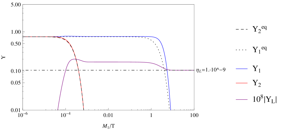
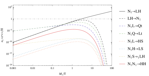
Refer to caption
(a) {M2,M1,K2,K1,K21,β}={109GeV,105GeV,8,0.2,40,50GeV}subscript𝑀2subscript𝑀1subscript𝐾2subscript𝐾1subscript𝐾21𝛽superscript109GeVsuperscript105GeV80.24050GeV\{M_{2},M_{1},K_{2},K_{1},K_{21},\beta\}=\{10^{9}\text{GeV},10^{5}\text{GeV},8,0.2,40,50\text{GeV}\}
Refer to caption
Refer to caption
Figure 11: These plots show a viable example of the high scale scenario. We show the evolution of the abundances and (rescaled) asymmetry (a), and the relative rates (b) as a function of temperature. In this regime, the CP𝐶𝑃CP-asymmetry is dominated by the standard Yukawa contribution, ϵimνMi/v2proportional-tosubscriptitalic-ϵ𝑖subscript𝑚𝜈subscript𝑀𝑖superscript𝑣2\epsilon_{i}\propto m_{\nu}M_{i}/v^{2}, and the final plot (c) displays the CP𝐶𝑃CP-asymmetries ϵ1,2subscriptitalic-ϵ12\epsilon_{1,2} as functions of M2subscript𝑀2M_{2}, for a constant mass ratio, M2/M1=104subscript𝑀2subscript𝑀1superscript104M_{2}/M_{1}=10^{4}. With a large mass hierarchy, there would be plenty of time for N1subscript𝑁1N_{1}-mediated processes to wash out all of the lepton asymmetry unless the N1subscript𝑁1N_{1} interactions are sufficiently suppressed, hence the very small Yukawa λ1subscript𝜆1\lambda_{1}.
Refer to caption
(a) {M2,M1,K2,K1,K21,β}={20TeV,2TeV,7,0.001,3105,50GeV}subscript𝑀2subscript𝑀1subscript𝐾2subscript𝐾1subscript𝐾21𝛽20TeV2TeV70.0013superscript10550GeV\{M_{2},M_{1},K_{2},K_{1},K_{21},\beta\}=\{20\text{TeV},2\text{TeV},7,0.001,3\cdot 10^{5},50\text{GeV}\}
Refer to caption
Refer to caption
Figure 12: These plots, in the same format as Fig. 11, show a viable example in the low mass regime. The hidden sector-sourced CP𝐶𝑃CP-asymmetry from N2subscript𝑁2N_{2} decays is the dominant contribution. The dominant scattering processes are also mediated by the hidden sector. This is also an explicit example of a scenario leading to a lepton asymmetry enhancement, thanks to the evolution traversing the sphaleron freezeout temperature.
  • High-scale models

    An example of a high scale scenario is shown in Fig. 11(a). The high mass regime is marked by the dominance of the Yukawa sector in contributing to the CP𝐶𝑃CP-asymmetry, so that ϵ2(3/16πv2)αmαM2ϵ1(M2/2M1)similar-tosubscriptitalic-ϵ2316𝜋superscript𝑣2subscript𝛼subscript𝑚𝛼subscript𝑀2similar-tosubscriptitalic-ϵ1subscript𝑀22subscript𝑀1\epsilon_{2}\sim(3/16\pi v^{2})\sum_{\alpha}m_{\alpha}M_{2}\sim\epsilon_{1}(M_{2}/2M_{1}), as displayed in Fig. 11. The general result in Eq. (57) reduces to

    YLL¯f9αmα64πv2M2(κ2e𝒵𝑑z(W1/z)+2M1M2κ1).similar-tosubscriptsuperscript𝑌𝑓𝐿¯𝐿9subscript𝛼subscript𝑚𝛼64𝜋superscript𝑣2subscript𝑀2subscript𝜅2superscript𝑒superscriptsubscript𝒵differential-dsuperscript𝑧subscript𝑊1superscript𝑧2subscript𝑀1subscript𝑀2subscript𝜅1Y^{f}_{L-\overline{L}}\sim\frac{9\sum_{\alpha}m_{\alpha}}{64\pi v^{2}}M_{2}\left(\kappa_{2}e^{-\int_{\mathcal{Z}}^{\infty}dz^{\prime}(W_{1}/z^{\prime})}+2\frac{M_{1}}{M_{2}}\kappa_{1}\right). (71)

    The lepton-number changing processes mediated by the hidden sector scale as |λ|2β2/M2similar-toabsentsuperscript𝜆2superscript𝛽2superscript𝑀2\sim|\lambda|^{2}\beta^{2}/M^{2}, and are suppressed compared to Yukawa-mediated scattering which scales as |λ|2mt2/v2similar-toabsentsuperscript𝜆2superscriptsubscript𝑚𝑡2superscript𝑣2\sim|\lambda|^{2}m_{t}^{2}/v^{2}. This is shown in Fig. 11. Additional scattering processes such as NiS𝑗LH𝑗absentsubscript𝑁𝑖𝑆𝐿𝐻N_{i}S\xrightarrow[j]{}LH scale as |α|2|λ|2superscript𝛼2superscript𝜆2|\alpha|^{2}|\lambda|^{2} and are therefore suppressed if |α|21much-less-thansuperscript𝛼21|\alpha|^{2}\ll 1, which holds for all the viable scenarios we consider here. The lepton-number conserving scattering process NiNiHHsubscript𝑁𝑖subscript𝑁𝑖𝐻𝐻N_{i}N_{i}\rightarrow HH, mediated by S𝑆S in the s𝑠s-channel, scales as |α|2β2/M2superscript𝛼2superscript𝛽2superscript𝑀2|\alpha|^{2}\beta^{2}/M^{2} and is again suppressed. Finally, the lepton-mediated t𝑡t-channel NiNiHHsubscript𝑁𝑖subscript𝑁𝑖𝐻𝐻N_{i}N_{i}\rightarrow HH scattering is suppressed by a factor |λ|21much-less-thansuperscript𝜆21|\lambda|^{2}\ll 1, and has no visible effect on the neutrino abundance.

    It follows that the efficiency factors κ1,2subscript𝜅12\kappa_{1,2} determined above can be used as a reasonably good approximation here, as the scattering corrections are small. Indeed, the dominant Nisubscript𝑁𝑖N_{i} scattering processes are controlled by the same equilibrium parameter Kisubscript𝐾𝑖K_{i}, and the Boltzmann-suppressed number density for T<Mi𝑇subscript𝑀𝑖T<M_{i} and the fast expansion rate at T>Mi𝑇subscript𝑀𝑖T>M_{i} limits their range of activity.

    The possibility of having ΔL=1,2Δ𝐿12\Delta L=1,2 scattering processes mediated by N1subscript𝑁1N_{1} that remain in equilibrium long after the lepton asymmetry YLL¯(2)subscriptsuperscript𝑌2𝐿¯𝐿Y^{(2)}_{L-\overline{L}} has been generated, is an important feature of HPL. In practice, these processes need to be suppressed, and remain out of equilibrium in viable models to avoid too much washout. For masses chosen so that β/M1mt/vmuch-less-than𝛽subscript𝑀1subscript𝑚𝑡𝑣\beta/M_{1}\ll m_{t}/v, the washout function is dominated by the Yukawa processes 𝒵𝑑z(W1/z)cK1similar-to-or-equalssuperscriptsubscript𝒵differential-dsuperscript𝑧subscript𝑊1superscript𝑧𝑐subscript𝐾1\int_{\mathcal{Z}}^{\infty}dz^{\prime}(W_{1}/z^{\prime})\simeq cK_{1}, where c1.2+1.4(mt/v)22.5similar-to𝑐1.21.4superscriptsubscript𝑚𝑡𝑣2similar-to2.5c\sim 1.2+1.4(m_{t}/v)^{2}\sim 2.5. With K2110similar-tosubscript𝐾2110K_{2}\sim 1-10, satisfying the neutrino mass constraint, one has κ21/(cK2)similar-tosubscript𝜅21𝑐subscript𝐾2\kappa_{2}\sim 1/(cK_{2}), and taking a mass ratio large enough that the κ1subscript𝜅1\kappa_{1} term can be neglected, we find the constraint

    YLL¯f9αmα64πv2M2ecK1cK2>ηL109.similar-tosubscriptsuperscript𝑌𝑓𝐿¯𝐿9subscript𝛼subscript𝑚𝛼64𝜋superscript𝑣2subscript𝑀2superscript𝑒𝑐subscript𝐾1𝑐subscript𝐾2subscript𝜂𝐿similar-to-or-equalssuperscript109Y^{f}_{L-\overline{L}}\sim\frac{9\sum_{\alpha}m_{\alpha}}{64\pi v^{2}}M_{2}\frac{e^{-cK_{1}}}{cK_{2}}>\eta_{L}\simeq 10^{-9}. (72)

    With the neutrino mass constraint αmαm3similar-tosubscript𝛼subscript𝑚𝛼subscript𝑚3\sum_{\alpha}m_{\alpha}\sim m_{3} as input, this implies the lower bound M2>(107GeV)cK2ecK1subscript𝑀2superscript107GeV𝑐subscript𝐾2superscript𝑒𝑐subscript𝐾1M_{2}>(10^{7}\text{GeV})\cdot cK_{2}e^{cK_{1}}. In standard one-flavor leptogenesis, we instead obtain the simpler bound, M1107greater-than-or-equivalent-tosubscript𝑀1superscript107M_{1}\gtrsim 10^{7}GeV. This is because the equilibrium parameter is constrained to satisfy K1<1subscript𝐾11K_{1}<1, so that κ11similar-tosubscript𝜅11\kappa_{1}\sim 1, and because scattering processes are not in equilibrium long enough to provide any significant washout.

  • Low-scale models

    A viable low scale example is shown in Fig. 12(a). The CP𝐶𝑃CP-asymmetry ϵ2subscriptitalic-ϵ2\epsilon_{2} for low values of M2subscript𝑀2M_{2} is controlled by the hidden sector couplings {α,β}𝛼𝛽\{\alpha,\beta\}, i.e. ϵ2(β/M2+|α21|/2)|α21|/r211/4proportional-tosubscriptitalic-ϵ2𝛽subscript𝑀2subscript𝛼212subscript𝛼21superscriptsubscript𝑟2114\epsilon_{2}\propto\left(\beta/M_{2}+|\alpha_{21}|/2\right)|\alpha_{21}|/r_{21}^{1/4}. At the same time, because the CP𝐶𝑃CP-asymmetry ϵ1subscriptitalic-ϵ1\epsilon_{1} is sourced purely from the Yukawa sector, it becomes negligible at low mass, ϵ1αmαM1/v2ϵ2proportional-tosubscriptitalic-ϵ1subscript𝛼subscript𝑚𝛼subscript𝑀1superscript𝑣2much-less-thansubscriptitalic-ϵ2\epsilon_{1}\propto\sum_{\alpha}m_{\alpha}M_{1}/v^{2}\ll\epsilon_{2}, as exemplified by Fig. 12. In this case, Eq. (57) reads,

    YLL¯f332πκ2(βM2+|α21|2)|α21|r211/4e𝒵𝑑z(W1/z).similar-to-or-equalssubscriptsuperscript𝑌𝑓𝐿¯𝐿332𝜋subscript𝜅2𝛽subscript𝑀2subscript𝛼212subscript𝛼21superscriptsubscript𝑟2114superscript𝑒superscriptsubscript𝒵differential-d𝑧subscript𝑊1superscript𝑧Y^{f}_{L-\overline{L}}\simeq\frac{3}{32\pi}\kappa_{2}\left(\frac{\beta}{M_{2}}+\frac{|\alpha_{21}|}{2}\right)\frac{|\alpha_{21}|}{r_{21}^{1/4}}e^{-\int_{\mathcal{Z}}^{\infty}dz(W_{1}/z^{\prime})}. (73)

    This relation relies on a hierarchical separation between the N2subscript𝑁2N_{2} and N1subscript𝑁1N_{1} phases, which is only marginally satisfied in Fig. 12(a) where M2/M1=10subscript𝑀2subscript𝑀110M_{2}/M_{1}=10. Nevertheless, the above relation encodes the two competing effects, namely the enhancement of the low-mass CP𝐶𝑃CP-asymmetry, and also the increased washout. Generating a larger CP𝐶𝑃CP-asymmetry requires an increase in the ratio β/M𝛽𝑀\beta/M, which at the same time increases the scattering rates and the washout (see the next subsection for details of the relative effects). Independent of the precise dynamics, for the relevant couplings, K2110similar-tosubscript𝐾2110K_{2}\sim 1-10, the efficiency factor will generally lie in the range κ20.010.5similar-tosubscript𝜅20.010.5\kappa_{2}\sim 0.01-0.5 (see Fig. 8). The washout function depends on the scattering processes, and we can approximate 𝒵𝑑zW1/z(3+2β/M1)K1similar-tosuperscriptsubscript𝒵differential-dsuperscript𝑧subscript𝑊1superscript𝑧32𝛽subscript𝑀1subscript𝐾1\int_{\cal Z}^{\infty}dz^{\prime}W_{1}/z^{\prime}\sim(3+2\beta/M_{1})K_{1}, so that exp(𝒵𝑑zW1/z)0.51similar-tosuperscriptsubscript𝒵differential-dsuperscript𝑧subscript𝑊1superscript𝑧0.51\exp(-\int_{\cal Z}^{\infty}dz^{\prime}W_{1}/z^{\prime})\sim 0.5-1 for K10.010.1similar-tosubscript𝐾10.010.1K_{1}\sim 0.01-0.1 and β/M11similar-to𝛽subscript𝑀11\beta/M_{1}\sim 1. As an example, taking κ2exp(𝒵𝑑zW1/z)0.1similar-tosubscript𝜅2superscriptsubscript𝒵differential-dsuperscript𝑧subscript𝑊1superscript𝑧0.1\kappa_{2}\exp(-\int_{\cal Z}^{\infty}dz^{\prime}W_{1}/z^{\prime})\sim 0.1 implies the following characteristic constraint on the lepton asymmetry,

    YLL¯f332π(βM2+|α21|2)|α21|r211/4101>ηL109,|α21|βM2M1M2>3107,formulae-sequencesimilar-tosubscriptsuperscript𝑌𝑓𝐿¯𝐿332𝜋𝛽subscript𝑀2subscript𝛼212subscript𝛼21superscriptsubscript𝑟2114superscript101subscript𝜂𝐿similar-to-or-equalssuperscript109subscript𝛼21𝛽subscript𝑀2subscript𝑀1subscript𝑀23superscript107Y^{f}_{L-\overline{L}}\sim\frac{3}{32\pi}\left(\frac{\beta}{M_{2}}+\frac{|\alpha_{21}|}{2}\right)\frac{|\alpha_{21}|}{r_{21}^{1/4}}10^{-1}>\eta_{L}\simeq 10^{-9},\qquad|\alpha_{21}|\frac{\beta}{M_{2}}\sqrt{\frac{M_{1}}{M_{2}}}>3\cdot 10^{-7}, (74)

    where small couplings |α21|β/M2much-less-thansubscript𝛼21𝛽subscript𝑀2|\alpha_{21}|\ll\beta/M_{2} have been assumed, and typically we will use |α21|105similar-tosubscript𝛼21superscript105|\alpha_{21}|\sim 10^{-5}. Given the above approximations, the light neutrino mass scale is a subleading parameter and does not appear in this bound.
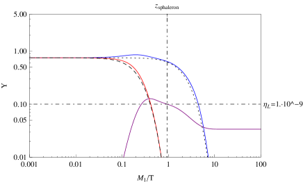
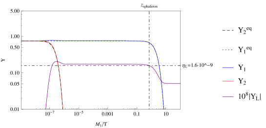
Refer to caption
(a) {M2,M1,K2,K1,K21,β}={1500GeV,155GeV,1,0.5,105,20GeV}subscript𝑀2subscript𝑀1subscript𝐾2subscript𝐾1subscript𝐾21𝛽1500GeV155GeV10.5superscript10520GeV\{M_{2},M_{1},K_{2},K_{1},K_{21},\beta\}=\{1500{\rm\,Ge\kern-1.0ptV},155{\rm\,Ge\kern-1.0ptV},1,0.5,10^{5},20{\rm\,Ge\kern-1.0ptV}\}
Refer to caption
(b) {M2,M1,K2,K1,K21,β}={109GeV,130GeV,8,0.5,4103,1GeV}subscript𝑀2subscript𝑀1subscript𝐾2subscript𝐾1subscript𝐾21𝛽superscript109GeV130GeV80.54superscript1031GeV\{M_{2},M_{1},K_{2},K_{1},K_{21},\beta\}=\newline \{10^{9}{\rm\,Ge\kern-1.0ptV},130{\rm\,Ge\kern-1.0ptV},8,0.5,4\cdot 10^{3},1{\rm\,Ge\kern-1.0ptV}\}
Figure 13: Scenarios representig low (a) and high (b) scale models which take advantage of the sphaleron cutoff temperature in order to liberate the parameters from stringent constraints.

An feature worth noting is the sensitivity to low temperature boundary conditions, namely the temperature at which B+L𝐵𝐿B+L-violating sphaleron transitions go out of equilibrium, Tsphaleron=159±1subscript𝑇𝑠𝑝𝑎𝑙𝑒𝑟𝑜𝑛plus-or-minus1591T_{sphaleron}=159\pm 1GeV D’Onofrio et al. (2014). The lepton asymmetry at this point effectively determines the final baryon asymmetry, while further evolution is observationally relatively unconstrained. This is phenomenologically interesting as it is usually quite difficult to find viable models with a large washout from N1subscript𝑁1N_{1}. However, if we choose M2subscript𝑀2M_{2} above and M1subscript𝑀1M_{1} well below the temperature at which sphaleron processes freeze out, the baryon asymmetry is generated right after N2subscript𝑁2N_{2} falls out-of-equilibrium, and will not be washed out at lower scales even if the lepton asymmetry is highly suppressed through N1subscript𝑁1N_{1} processes. The N1subscript𝑁1N_{1} sector effectively decouples in this case. A low mass example is shown in Fig. 13(a). Note that Tsphaleron>M1>mHsubscript𝑇𝑠𝑝𝑎𝑙𝑒𝑟𝑜𝑛subscript𝑀1subscript𝑚𝐻T_{sphaleron}>M_{1}>m_{H} in this case, since M1<mHsubscript𝑀1subscript𝑚𝐻M_{1}<m_{H} would require the inclusion of interactions such as N1LHsubscript𝑁1𝐿𝐻N_{1}L\leftrightarrow H, that have not been considered thus far.444Note that such processes may also arise on including thermal corrections to the scalar masses. In the low mass regime, many interactions are relevant which cause significant washout of the lepton asymmetry. As a consequence, the range of parameters available for low mass scenarios is quite limited. On the other hand, an example of a high mass scenario which also takes advantage of the sphaleron cutoff temperature is shown in figure Fig. 13(b). In that situation, all of the lepton asymmetry is generated out of the first phase, from N2subscript𝑁2N_{2} leptonic decays. In this case, with M1<Tsphaleronsubscript𝑀1subscript𝑇𝑠𝑝𝑎𝑙𝑒𝑟𝑜𝑛M_{1}<T_{sphaleron}, the physics of N1subscript𝑁1N_{1}, including the hidden sector interactions, are only weakly constrained. An interesting aspect of this scenario is the possibility of exploring models where the lightest RH neutrino is so light and weakly coupled to leptons, that its lifetime could be long enough to play an independent cosmological role, potentially in the form of sterile neutrino dark matter Kusenko (2009); *Petraki:2007gq. In such cases, the N1subscript𝑁1N_{1} abundance will have to be sufficiently depleted for consistency with constraints on the dark matter abundance. This can be achieved through adjusting the N1N1HHsubscript𝑁1subscript𝑁1𝐻𝐻N_{1}N_{1}\rightarrow HH rate.

4.2 Aspects of the dynamics
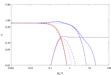
Refer to caption
(a) {M2,M1,K2,K1,K21,β}={108GeV,104GeV,0.8,0.4,4102,50GeV}subscript𝑀2subscript𝑀1subscript𝐾2subscript𝐾1subscript𝐾21𝛽superscript108GeVsuperscript104GeV0.80.44superscript10250GeV\{M_{2},M_{1},K_{2},K_{1},K_{21},\beta\}=\newline \{10^{8}{\rm\,Ge\kern-1.0ptV},10^{4}{\rm\,Ge\kern-1.0ptV},0.8,0.4,4\cdot 10^{2},50{\rm\,Ge\kern-1.0ptV}\}
Refer to caption
(b) {M2,M1,K2,K1,K21,β}={2103GeV,200GeV,0.8,0.04,400,500GeV}subscript𝑀2subscript𝑀1subscript𝐾2subscript𝐾1subscript𝐾21𝛽2superscript103GeV200GeV0.80.04400500GeV\{M_{2},M_{1},K_{2},K_{1},K_{21},\beta\}=\newline \{2\cdot 10^{3}{\rm\,Ge\kern-1.0ptV},200{\rm\,Ge\kern-1.0ptV},0.8,0.04,400,500{\rm\,Ge\kern-1.0ptV}\}
Figure 14: Plots showing the impact of ΔL=1Δ𝐿1\Delta L=1 and ΔN=2Δ𝑁2\Delta N=2 processes on the dynamics for high scales {M2,M1}={108,104}subscript𝑀2subscript𝑀1superscript108superscript104\{M_{2},M_{1}\}=\{10^{8},10^{4}\}GeV (on the left) and low scales {M2,M1}={2,0.2}subscript𝑀2subscript𝑀120.2\{M_{2},M_{1}\}=\{2,0.2\}TeV (on the right). The color coding, blue, red, purple and black, is the same as in Fig. 11(a) 12(a),  13(a). The dotted pattern is for decays only, dashed for decays plus ΔL=1Δ𝐿1\Delta L=1 scattering, and plain for decays plus ΔL=1Δ𝐿1\Delta L=1 and ΔN=2Δ𝑁2\Delta N=2 scattering.
Refer to caption
(a) K2={0.1,5,10}subscript𝐾20.1510K_{2}=\{0.1,5,10\} (plain, dashed, dotted)
Refer to caption
(b) K1={0.1,5,10}subscript𝐾10.1510K_{1}=\{0.1,5,10\} (plain, dashed, dotted)
Refer to caption
(c) K2={0.1,5,10}subscript𝐾20.1510K_{2}=\{0.1,5,10\} (plain, dashed, dotted)
Refer to caption
(d) K1={0.1,5,10}subscript𝐾10.1510K_{1}=\{0.1,5,10\} (plain, dashed, dotted)
Refer to caption
(e) K21={10,500,1000}subscript𝐾21105001000K_{21}=\{10,500,1000\} (plain, dashed, dotted)
Refer to caption
(f) β={10,500,1000}𝛽105001000\beta=\{10,500,1000\}GeV (plain, dashed, dotted)
Figure 15: The effect of {K2,K1,K21,β}subscript𝐾2subscript𝐾1subscript𝐾21𝛽\{K_{2},K_{1},K_{21},\beta\} on the dynamics for high {M2,M1}={108,104}subscript𝑀2subscript𝑀1superscript108superscript104\{M_{2},M_{1}\}=\{10^{8},10^{4}\}GeV (top two plots), and low {M2,M1}={2,0.2}subscript𝑀2subscript𝑀120.2\{M_{2},M_{1}\}=\{2,0.2\}TeV (bottom four plots) mass regimes. The color coding, blue, red, purple and black, is the same as Fig. 11(a) 12(a),  13(a), while the dotted, dashed and plain lines represent the variation of each parameter.

In this subsection, we relax some of the constraints required for physical scenarios and focus on the various dynamical components that come into play: the decays and scattering processes on one hand, and the various parameters on the other.

Decays and inverse decays versus scattering

The impact of the decays, inverse decays and scattering is summarized in Fig. 14. We overlay three solutions: (i) just decays and inverse decays (dotted lines), (ii) decays, inverse decays and ΔL=1Δ𝐿1\Delta L=1 scattering (dashed lines), and finally (iii) decays, inverse decays and ΔL=1Δ𝐿1\Delta L=1 and ΔN=2Δ𝑁2\Delta N=2 scattering (plain lines).

Starting with the high mass regime, the hidden sector scattering processes, e.g. NiHLSsubscript𝑁𝑖𝐻𝐿𝑆N_{i}H\rightarrow LS, NiNiHHsubscript𝑁𝑖subscript𝑁𝑖𝐻𝐻N_{i}N_{i}\rightarrow HH, are subdominant compared to the Yukawa-mediated processes since β/Mimt/vmuch-less-than𝛽subscript𝑀𝑖subscript𝑚𝑡𝑣\beta/M_{i}\ll m_{t}/v. This can be seen from Fig. 14(a), where ΔL=1Δ𝐿1\Delta L=1 scattering has a significant effect relative to decays, whereas the ΔN=2Δ𝑁2\Delta N=2 scatterings have no visible effect. In practice, the decays and inverse decays remain the dominant effect, and the results from section 3.2 can be reasonably well applied.

The low mass regime is marked instead by the significant, if not dominant, effect of hidden sector scattering processes, given β/Mimt/vsimilar-to𝛽subscript𝑀𝑖subscript𝑚𝑡𝑣\beta/M_{i}\sim m_{t}/v. Looking at the plot in Fig. 14(b), the effect of adding ΔL=1Δ𝐿1\Delta L=1 scattering is similar to that in the high mass regime, however the impact of ΔN=2Δ𝑁2\Delta N=2 processes is greatly enhanced. Although these processes do not violate lepton number, ΔL=0Δ𝐿0\Delta L=0, they act to maintain the neutrino abundance closer to equilibrium. As a consequence, both the ΔL=1Δ𝐿1\Delta L=1 processes (e.g. decays) and the inverse processes (e.g. inverse decays) remain in equilibrium for longer, leading to an enhanced lepton washout in that regime.

Parameter Dependence

The dependence of the dynamics on the parameters is displayed in Fig. 15. The subsection above considered examples of viable models that satisfy the basic constraints, and focused on constraining the relevant parameters accordingly. We now ignore those constraints, and instead vary the parameters {K2,K1,K21,β}subscript𝐾2subscript𝐾1subscript𝐾21𝛽\{K_{2},K_{1},K_{21},\beta\} to study their impact in both high and low mass regimes.

  • {K2,K1}subscript𝐾2subscript𝐾1\{K_{2},K_{1}\}:- Figs. 15(a) and 15(b) exhibit the effects of K2subscript𝐾2K_{2} and K1subscript𝐾1K_{1} in the large mass regime. When the N1subscript𝑁1N_{1} and N2subscript𝑁2N_{2} phases can be hierarchically separated, they both act as independent one flavor systems according to the respective efficiency factors κ1,2subscript𝜅12\kappa_{1,2}. Consequently, we expect little deviation from the toy model that was studied previously.

    Figs. 15(c) and 15(d) exhibit the effects of K2subscript𝐾2K_{2} and K1subscript𝐾1K_{1} in the low mass regime. This regime requires a smaller mass ratio to achieve sufficient CP𝐶𝑃CP-asymmetry, therefore the overlap of the N2subscript𝑁2N_{2} and N1subscript𝑁1N_{1} phases induces more intricate dynamics, though we observe that the impact of K2subscript𝐾2K_{2} and K1subscript𝐾1K_{1} can still be separated.

  • {K21,β}subscript𝐾21𝛽\{K_{21},\beta\}:- Figs. 15(e) and 15(f) exhibit the effects of varying K21subscript𝐾21K_{21} and β𝛽\beta in the low mass scale regime. The primary effect is on the magnitude of the lepton asymmetry, via the impact on the CP𝐶𝑃CP-asymmetry of N2subscript𝑁2N_{2}. However, there are also effects due to scattering. Indeed, in both cases the maximal lepton asymmetry is achieved for mid-range values, K21=500subscript𝐾21500K_{21}=500 and β=500𝛽500\beta=500GeV respectively. This illustrates the fact that beyond a given threshold, increasing these parameters increases the scattering washout more significantly which more than compensates for the increase in the CP𝐶𝑃CP-asymmetry.

5 Concluding Remarks

This paper has considered a minimal extension of leptogenesis that arises by opening up the Higgs portal with a new singlet scalar. This scalar can also couple at the renormalizable level to the RH neutrinos which introduces a new (hidden sector) source of CP𝐶𝑃CP violation into the theory. The new RHN decay channels that are opened allow Higgs portal leptogenesis to avoid the stringent constraints of the Davidson-Ibarra bound, with viable low scale scenarios that we have considered in detail. The new decay channels are only available for the next-to-lightest RH neutrinos, which has a number of interesting implications for phenomenology. We conclude in this section by mentioning a number of these as directions for future work.

  • First-order leptogenesis: The new decay channels, e.g. N2N1+Ssubscript𝑁2subscript𝑁1𝑆N_{2}\rightarrow N_{1}+S do not violate lepton number. Thus, this model falls into a general category in which the next-to-lightest RH neutrinos have both L𝐿L-violating and L𝐿L-conserving decays. As has recently been emphasized Bhattacharya et al. (2014), such models allow the original Weinberg-Nanopoulos theorem Nanopoulos and Weinberg (1979) to be evaded in that the loop-level amplitude can be of first-order in the L𝐿L-violating vertex. This is clear from the analysis in Section 2, and thus the HPL model is a simple example illustrating this general feature.

  • Light (CP𝐶𝑃CP violating) sterile neutrinos: Since the new sources of the CP𝐶𝑃CP-asymmetry arise from decays of the next-to-lightest RH neutrino states, it is possible to effectively decouple N1subscript𝑁1N_{1} from leptogenesis. Indeed, since the normal heirarchy still allows one parametrically light (or massless) active neutrino, we can consider taking N1subscript𝑁1N_{1} to be, for example, in the keV mass range for sterile neutrino dark matter. It would be interesting to explore whether the washout constraints on the interactions allow for viable thermal production modes in the early universe. It is notable that, since αijsubscript𝛼𝑖𝑗\alpha_{ij} contains multiple CP𝐶𝑃CP-odd phases, this model would generically imply some new low energy contributions (albeit suppressed) to CP𝐶𝑃CP-violating observables.

  • Dynamical seesaw scale: We assumed throughout that the scalar S𝑆S was in a stable vacuum throughout the range of cosmological evolution relevant for leptogenesis. This needn’t be the case, and the full scalar potential V(H,S)𝑉𝐻𝑆V(H,S) could allow for some evolution in Sdelimited-⟨⟩𝑆\langle S\rangle, which would in turn affect the RH neutrino mass scale. Some of these issues were recently considered in Aristizabal Sierra et al. (2014), and it would be interesting to explore the implications of having an early epoch where, for example, the RH neutrino mass scale were to pass through zero due to a phase transition in the scalar potential.555We thank Maxim Pospelov for suggesting this possibility, and related discussions.

Acknowledgements

We would like to thank M. Pospelov for many helpful discussions. The work of M.L. and A.R. is supported in part by NSERC, Canada.


Appendix A Parametrization of the CP-asymmetry

The focus of this paper is on the dynamics of the Boltzmann evolution for HPL and the dependence on the masses and mass ratios. Therefore, rather than working with the full CP𝐶𝑃CP-asymmetries computed in Section 2, in this Appendix we will derive an order-of-magnitude estimate that will be more convenient to use in exploring the full evolution. To this end, we replace the coupling constants by their magnitudes, enabling components from the different chirality chains to be combined. Doing so effectively gives us an absolute upper bound on the asymmetries.

Hidden sector CP𝐶𝑃CP asymmetry

Starting with the hidden sector, and using the forms (19) and (23) for the vertex and wave function corrections, we write

|ϵiv|j|(λλ)ji|(λλ)ii|αij|8πβMi(jLLv+jRLv),|ϵiw|l,j|(λλ)ji|(λλ)ii|αljαil|8π(jlLLw+jlRLw+jlLRw+jlRRw).formulae-sequencesimilar-tosuperscriptsubscriptitalic-ϵ𝑖𝑣subscript𝑗subscriptsuperscript𝜆𝜆𝑗𝑖subscriptsuperscript𝜆𝜆𝑖𝑖subscript𝛼𝑖𝑗8𝜋𝛽subscript𝑀𝑖subscriptsuperscript𝑣𝑗𝐿𝐿subscriptsuperscript𝑣𝑗𝑅𝐿similar-tosuperscriptsubscriptitalic-ϵ𝑖𝑤subscript𝑙𝑗subscriptsuperscript𝜆𝜆𝑗𝑖subscriptsuperscript𝜆𝜆𝑖𝑖subscript𝛼𝑙𝑗subscript𝛼𝑖𝑙8𝜋subscriptsuperscript𝑤𝑗𝑙𝐿𝐿subscriptsuperscript𝑤𝑗𝑙𝑅𝐿subscriptsuperscript𝑤𝑗𝑙𝐿𝑅subscriptsuperscript𝑤𝑗𝑙𝑅𝑅\begin{split}&|\epsilon_{i}^{v}|\sim\sum_{j}\frac{|(\lambda^{\dagger}\lambda)_{ji}|}{(\lambda^{\dagger}\lambda)_{ii}}\frac{|\alpha_{ij}|}{8\pi}\frac{\beta}{M_{i}}\left(\mathcal{F}^{v}_{jLL}+\mathcal{F}^{v}_{jRL}\right),\\ &|\epsilon_{i}^{w}|\sim\sum_{l,j}\frac{|(\lambda^{\dagger}\lambda)_{ji}|}{(\lambda^{\dagger}\lambda)_{ii}}\frac{|\alpha_{lj}\alpha_{il}|}{8\pi}\left(\mathcal{F}^{w}_{jlLL}+\mathcal{F}^{w}_{jlRL}+\mathcal{F}^{w}_{jlLR}+\mathcal{F}^{w}_{jlRR}\right).\end{split} (75)

Assuming the standard see-saw mechanism, we can replace the Yukawa couplings by the light active neutrino masses through the following relations Casas and Ibarra (2001),

mν=v2λM1λ,λ=1vUDmRDM,formulae-sequencesubscript𝑚𝜈superscript𝑣2superscript𝜆superscript𝑀1superscript𝜆𝜆1𝑣𝑈subscript𝐷𝑚superscript𝑅subscript𝐷𝑀m_{\nu}=v^{2}\lambda^{*}M^{-1}\lambda^{\dagger},\qquad\lambda=\frac{1}{v}UD_{\sqrt{m}}R^{\dagger}D_{\sqrt{M}}, (76)

where the Higgs vacuum expectation value is v=174𝑣174v=174\,GeV, and R𝑅R is a (complex) orthogonal matrix, and the diagonal Majorana and active neutrino mass matrices are respectively DM=diag(M1,M2,M3)subscript𝐷𝑀diagsubscript𝑀1subscript𝑀2subscript𝑀3D_{M}=\text{diag}(M_{1},M_{2},M_{3}), and Dm=diag(m1,m2,m3)subscript𝐷𝑚diagsubscript𝑚1subscript𝑚2subscript𝑚3D_{m}=\text{diag}(m_{1},m_{2},m_{3}). The matrix U𝑈U is the so-called unitary PMNS matrix. Using this notation, we can write

(λλ)ji=MiMjv2bmbRjbRib,(λλ)ii=Miv2bmb|Rib|2.formulae-sequencesubscriptsuperscript𝜆𝜆𝑗𝑖subscript𝑀𝑖subscript𝑀𝑗superscript𝑣2subscript𝑏subscript𝑚𝑏subscript𝑅𝑗𝑏superscriptsubscript𝑅𝑖𝑏subscriptsuperscript𝜆𝜆𝑖𝑖subscript𝑀𝑖superscript𝑣2subscript𝑏subscript𝑚𝑏superscriptsubscript𝑅𝑖𝑏2(\lambda^{\dagger}\lambda)_{ji}=\frac{\sqrt{M_{i}M_{j}}}{v^{2}}\sum_{b}m_{b}R_{jb}R_{ib}^{*},\qquad(\lambda^{\dagger}\lambda)_{ii}=\frac{M_{i}}{v^{2}}\sum_{b}m_{b}|R_{ib}|^{2}. (77)

The Schwartz inequality |bmbRjbRib|2αmα|Rjα|2βmβ|Riβ|2superscriptsubscript𝑏subscript𝑚𝑏subscript𝑅𝑗𝑏subscriptsuperscript𝑅𝑖𝑏2subscript𝛼subscript𝑚𝛼superscriptsubscript𝑅𝑗𝛼2subscript𝛽subscript𝑚𝛽superscriptsubscript𝑅𝑖𝛽2|\sum_{b}m_{b}R_{jb}R^{*}_{ib}|^{2}\leq\sum_{\alpha}m_{\alpha}|R_{j\alpha}|^{2}\sum_{\beta}m_{\beta}|R_{i\beta}|^{2}, then allows the couplings to be bounded from above

|(λλ)ji|(λλ)iiMjbmb|Rjb|2Mibmb|Rib|2MjMi.less-than-or-similar-tosubscriptsuperscript𝜆𝜆𝑗𝑖subscriptsuperscript𝜆𝜆𝑖𝑖subscript𝑀𝑗subscript𝑏subscript𝑚𝑏superscriptsubscript𝑅𝑗𝑏2subscript𝑀𝑖subscript𝑏subscript𝑚𝑏superscriptsubscript𝑅𝑖𝑏2similar-tosubscript𝑀𝑗subscript𝑀𝑖\frac{|(\lambda^{\dagger}\lambda)_{ji}|}{(\lambda^{\dagger}\lambda)_{ii}}\lesssim\sqrt{\frac{M_{j}\sum_{b}m_{b}|R_{jb}|^{2}}{M_{i}\sum_{b}m_{b}|R_{ib}|^{2}}}\sim\sqrt{\frac{M_{j}}{M_{i}}}. (78)

The final approximation assumes all the entries of the orthogonal matrix R𝑅R are similar in magnitude. When R𝑅R is real, the orthogonality condition RTR=1superscript𝑅𝑇𝑅1R^{T}R=\textbf{1} ensures that its elements satisfy Rij1subscript𝑅𝑖𝑗1R_{ij}\leqslant 1. When R𝑅R is complex, we have fewer constraints but bounding |Rij|subscript𝑅𝑖𝑗|R_{ij}| by unity is a sufficient condition for orthogonality, and to obtain a characteristic estimate below we will simply assume |Rij|1similar-tosubscript𝑅𝑖𝑗1|R_{ij}|\sim 1.

Because of kinematic constraints, we have ϵ1=0subscriptitalic-ϵ10\epsilon_{1}=0. For i=2𝑖2i=2, the neutrino sum runs over j=1,3𝑗13j=1,3. However, the asymmetry vanishes when j=3𝑗3j=3, since M3>M2subscript𝑀3subscript𝑀2M_{3}>M_{2} is kinematically forbidden for the cut loop. The sum thus reduces to j=1𝑗1j=1 only. For the wave-function corrections, we have two sums over j,l=1,3formulae-sequence𝑗𝑙13j,l=1,3. The index j𝑗j denotes the neutrino inside the loop, and is therefore constrained to j=1𝑗1j=1 by the cut kinematics, but l=3𝑙3l=3 is not forbidden. However by assumption r321much-greater-thansubscript𝑟321r_{32}\gg 1, and in that limit the resulting CP-asymmetry is negligible. The sums therefore collapse to j=l=1𝑗𝑙1j=l=1. Hence, we arrive at the parametric estimate,

ϵ2v|α21|8πβM2M1M2(jLLv+jRLv),ϵ2w|α11α21|8πM1M2(jlLLw+jlRLw+jlLRw+jlRRw),formulae-sequencesimilar-tosuperscriptsubscriptitalic-ϵ2𝑣subscript𝛼218𝜋𝛽subscript𝑀2subscript𝑀1subscript𝑀2subscriptsuperscript𝑣𝑗𝐿𝐿subscriptsuperscript𝑣𝑗𝑅𝐿similar-tosuperscriptsubscriptitalic-ϵ2𝑤subscript𝛼11subscript𝛼218𝜋subscript𝑀1subscript𝑀2subscriptsuperscript𝑤𝑗𝑙𝐿𝐿subscriptsuperscript𝑤𝑗𝑙𝑅𝐿subscriptsuperscript𝑤𝑗𝑙𝐿𝑅subscriptsuperscript𝑤𝑗𝑙𝑅𝑅\begin{split}&\epsilon_{2}^{v}\sim\frac{|\alpha_{21}|}{8\pi}\frac{\beta}{M_{2}}\sqrt{\frac{M_{1}}{M_{2}}}\left(\mathcal{F}^{v}_{jLL}+\mathcal{F}^{v}_{jRL}\right),\\ &\epsilon_{2}^{w}\sim\frac{|\alpha_{11}\alpha_{21}|}{8\pi}\sqrt{\frac{M_{1}}{M_{2}}}\left(\mathcal{F}^{w}_{jlLL}+\mathcal{F}^{w}_{jlRL}+\mathcal{F}^{w}_{jlLR}+\mathcal{F}^{w}_{jlRR}\right),\end{split} (79)

The functions \mathcal{F} depend upon the variable 1/r211subscript𝑟211/r_{21}, which tends to zero in the hierarchical regime, r211much-greater-thansubscript𝑟211r_{21}\gg 1. In that limit, we find the asymptotic behaviour

ϵ2v|α21|8πβM2M1M2(1σ2),ϵ2w|α11α21|16πM1M2(1σ2)2.formulae-sequencesimilar-tosuperscriptsubscriptitalic-ϵ2𝑣subscript𝛼218𝜋𝛽subscript𝑀2subscript𝑀1subscript𝑀21subscript𝜎2similar-tosuperscriptsubscriptitalic-ϵ2𝑤subscript𝛼11subscript𝛼2116𝜋subscript𝑀1subscript𝑀2superscript1subscript𝜎22\begin{split}&\epsilon_{2}^{v}\sim\frac{|\alpha_{21}|}{8\pi}\frac{\beta}{M_{2}}\sqrt{\frac{M_{1}}{M_{2}}}(1-\sigma_{2}),\\ &\epsilon_{2}^{w}\sim\frac{|\alpha_{11}\alpha_{21}|}{16\pi}\sqrt{\frac{M_{1}}{M_{2}}}(1-\sigma_{2})^{2}.\end{split} (80)

In Fig. 16, we compare the above approximate functions with the exact functions calculated in the main text, cf. Eqs. (19), (23). The approximations are excellent for large M2/M1subscript𝑀2subscript𝑀1M_{2}/M_{1}, but only deviate from the exact answer by a factor of 2 for M2/M110greater-than-or-equivalent-tosubscript𝑀2subscript𝑀110M_{2}/M_{1}\gtrsim 10.

Refer to caption
Refer to caption
Figure 16: Plots of the full loop functions {\cal F} (solid), and the approximations (dashed) discussed in this section, as a function of the RHN mass hierarchy.
Refer to caption
Figure 17: The differing contributions to the total CP𝐶𝑃CP-asymmetry ϵ2subscriptitalic-ϵ2\epsilon_{2} for various mass ratios M2/M1subscript𝑀2subscript𝑀1M_{2}/M_{1}. The high mass ratio is dominated by the Yukawa-sourced CP𝐶𝑃CP-asymmetry, ϵ0αmαM2/v2proportional-tosubscriptitalic-ϵ0subscript𝛼subscript𝑚𝛼subscript𝑀2superscript𝑣2\epsilon_{0}\propto\sum_{\alpha}m_{\alpha}M_{2}/v^{2} (black, dot-dashed line). The low mass CP𝐶𝑃CP-asymmetry is proportional to the β𝛽\beta coupling via the vertex correction, ϵ(β)M1/M2|αβ|/M2similar-tosubscriptitalic-ϵ𝛽subscript𝑀1subscript𝑀2𝛼𝛽subscript𝑀2\epsilon_{(\beta)}\sim\sqrt{M_{1}/M_{2}}|\alpha\beta|/M_{2} (dotted lines). In the intermediate mass range, the CP𝐶𝑃CP-asymmetry is dominantly generated by the wave function correction ϵ(α)|α|2M1/M2similar-tosubscriptitalic-ϵ𝛼superscript𝛼2subscript𝑀1subscript𝑀2\epsilon_{(\alpha)}\sim|\alpha|^{2}\sqrt{M_{1}/M_{2}} (dashed lines).

Standard Yukawa CP𝐶𝑃CP asymmetry

We also recall the conventional contribution to the CP𝐶𝑃CP-asymmetry, ϵ0subscriptitalic-ϵ0\epsilon_{0} Covi et al. (1996); Roulet et al. (1998); Buchmuller and Plumacher (1998); Pilaftsis (1997). In general, the loop-induced vertex and wave-function contributions from Nisubscript𝑁𝑖N_{i} decays are,

ϵ0iv=jiIm{(λλ)ji2}8π(λλ)ii0v(rji),ϵ0iw=jiIm{(λλ)ji2}8π(λλ)ii0w(rji),formulae-sequencesubscriptsuperscriptitalic-ϵ𝑣0𝑖subscript𝑗𝑖Imsuperscriptsubscriptsuperscript𝜆𝜆𝑗𝑖28𝜋subscriptsuperscript𝜆𝜆𝑖𝑖subscriptsuperscript𝑣0subscript𝑟𝑗𝑖subscriptsuperscriptitalic-ϵ𝑤0𝑖subscript𝑗𝑖Imsuperscriptsubscriptsuperscript𝜆𝜆𝑗𝑖28𝜋subscriptsuperscript𝜆𝜆𝑖𝑖subscriptsuperscript𝑤0subscript𝑟𝑗𝑖\epsilon^{v}_{0i}=\sum_{j\neq i}\frac{\text{Im}\{(\lambda^{\dagger}\lambda)_{ji}^{2}\}}{8\pi(\lambda^{\dagger}\lambda)_{ii}}\mathcal{F}^{v}_{0}(r_{ji}),\qquad\epsilon^{w}_{0i}=\sum_{j\neq i}\frac{\text{Im}\{(\lambda^{\dagger}\lambda)_{ji}^{2}\}}{8\pi(\lambda^{\dagger}\lambda)_{ii}}\mathcal{F}^{w}_{0}(r_{ji}), (81)

with

0v(rji)=rji[1(1+rji)log(1+rjirji)],0w(rji)=rji(1rji).formulae-sequencesubscriptsuperscript𝑣0subscript𝑟𝑗𝑖subscript𝑟𝑗𝑖delimited-[]11subscript𝑟𝑗𝑖1subscript𝑟𝑗𝑖subscript𝑟𝑗𝑖subscriptsuperscript𝑤0subscript𝑟𝑗𝑖subscript𝑟𝑗𝑖1subscript𝑟𝑗𝑖\mathcal{F}^{v}_{0}(r_{ji})=\sqrt{r_{ji}}\left[1-(1+r_{ji})\log\left(\frac{1+r_{ji}}{r_{ji}}\right)\right],\qquad\mathcal{F}^{w}_{0}(r_{ji})=\frac{\sqrt{r_{ji}}}{(1-r_{ji})}. (82)

Using Eq. (77) and the Schwartz inequality, we can again relate the Yukawa coupling to the light neutrino masses, and bound from above the magnitude of the CP𝐶𝑃CP-asymmetry. Taking |Rij|1similar-tosubscript𝑅𝑖𝑗1|R_{ij}|\sim 1, we find

|ϵ0i|αmα8πv2jiMj|0v(rji)+0w(rji)|.similar-tosubscriptitalic-ϵ0𝑖subscript𝛼subscript𝑚𝛼8𝜋superscript𝑣2subscript𝑗𝑖subscript𝑀𝑗subscriptsuperscript𝑣0subscript𝑟𝑗𝑖subscriptsuperscript𝑤0subscript𝑟𝑗𝑖|\epsilon_{0i}|\sim\frac{\sum_{\alpha}m_{\alpha}}{8\pi v^{2}}\sum_{j\neq i}M_{j}\left|\mathcal{F}^{v}_{0}(r_{ji})+\mathcal{F}^{w}_{0}(r_{ji})\right|. (83)

The sum over the active neutrino masses is constrained by cosmological data, with bounds in the range αmα<0.21subscript𝛼subscript𝑚𝛼0.21\sum_{\alpha}m_{\alpha}<0.2-1eV Ade et al. (2013); Moresco et al. (2012); *Xia:2012na; *Giusarma:2013pmn. The additional assumption of a normal hierarchy leads to a stronger constraint αmαm3Δm3120.040.05greater-than-or-equivalent-tosubscript𝛼subscript𝑚𝛼subscript𝑚3similar-to-or-equalsΔsuperscriptsubscript𝑚312similar-to-or-equals0.040.05\sum_{\alpha}m_{\alpha}\gtrsim m_{3}\simeq\sqrt{\Delta m_{31}^{2}}\simeq 0.04-0.05eV at the 3σ𝜎\sigma level Capozzi et al. (2014); *Fogli:2012ua; *GonzalezGarcia:2012sz; *Tortola:2012te. Throughout this paper, we assume a normal hierarchy for the light neutrinos, taking αmαm30.05similar-tosubscript𝛼subscript𝑚𝛼subscript𝑚3similar-to0.05\sum_{\alpha}m_{\alpha}\sim m_{3}\sim 0.05eV. When the internal RHN is much heavier than the external neutrino, so that rji1much-greater-thansubscript𝑟𝑗𝑖1r_{ji}\gg 1, the loop function has the limit |0v+0w|3/(2rji)similar-tosubscriptsuperscript𝑣0subscriptsuperscript𝑤032subscript𝑟𝑗𝑖|\mathcal{F}^{v}_{0}+\mathcal{F}^{w}_{0}|\sim 3/(2\sqrt{r_{ji}}). At the other end of the spectrum, when the internal RHN is much lighter, rji1much-less-thansubscript𝑟𝑗𝑖1r_{ji}\ll 1, we find |0v+0w|rji|2+log(rji)|similar-tosubscriptsuperscript𝑣0subscriptsuperscript𝑤0subscript𝑟𝑗𝑖2subscript𝑟𝑗𝑖|\mathcal{F}^{v}_{0}+\mathcal{F}^{w}_{0}|\sim\sqrt{r_{ji}}|2+\log(r_{ji})|, as shown in Fig. 16. The CP𝐶𝑃CP-asymmetry from N1subscript𝑁1N_{1} decays receives contributions from internal j=2,3𝑗23j=2,3 heavy neutrinos, which imply j=2,3Mj|0v(rj1)+0w(rj1)|3M1similar-tosubscript𝑗23subscript𝑀𝑗subscriptsuperscript𝑣0subscript𝑟𝑗1subscriptsuperscript𝑤0subscript𝑟𝑗13subscript𝑀1\sum_{j=2,3}M_{j}\left|\mathcal{F}^{v}_{0}(r_{j1})+\mathcal{F}^{w}_{0}(r_{j1})\right|\sim 3M_{1}. The CP𝐶𝑃CP-asymmetry from N2subscript𝑁2N_{2} decays receives a contribution from j=3𝑗3j=3 giving 3M2/23subscript𝑀223M_{2}/2, and a contribution from j=1𝑗1j=1 giving M2(M12/M22)|log(M22/M12)|M2much-less-thansubscript𝑀2superscriptsubscript𝑀12superscriptsubscript𝑀22subscriptsuperscript𝑀22subscriptsuperscript𝑀21subscript𝑀2M_{2}(M_{1}^{2}/M_{2}^{2})|\log(M^{2}_{2}/M^{2}_{1})|\ll M_{2}, which is neglected. In total, we obtain the standard parametric scaling of the CP𝐶𝑃CP-asymmetry,

|ϵ01|3M1αmα8πv2,|ϵ02|3M2αmα16πv2.formulae-sequencesimilar-tosubscriptitalic-ϵ013subscript𝑀1subscript𝛼subscript𝑚𝛼8𝜋superscript𝑣2similar-tosubscriptitalic-ϵ023subscript𝑀2subscript𝛼subscript𝑚𝛼16𝜋superscript𝑣2|\epsilon_{01}|\sim\frac{3M_{1}\sum_{\alpha}m_{\alpha}}{8\pi v^{2}},\qquad|\epsilon_{02}|\sim\frac{3M_{2}\sum_{\alpha}m_{\alpha}}{16\pi v^{2}}. (84)

This is analogous to the Davidson-Ibarra bound Davidson and Ibarra (2002), though somewhat less strict as it depends on αmαsubscript𝛼subscript𝑚𝛼\sum_{\alpha}m_{\alpha} rather than m3m1subscript𝑚3subscript𝑚1m_{3}-m_{1}, which is a consequence of taking |Rij|1similar-tosubscript𝑅𝑖𝑗1|R_{ij}|\sim 1. In the standard case one can go further as the CP𝐶𝑃CP-asymmetry is sensitive to the (λλ)ij2subscriptsuperscriptsuperscript𝜆𝜆2𝑖𝑗(\lambda^{\dagger}\lambda)^{2}_{ij} elements which depend on Rij2superscriptsubscript𝑅𝑖𝑗2R_{ij}^{2}, as can seen from the representation in (77). Thus, the orthogonality condition kRki2=1subscript𝑘superscriptsubscript𝑅𝑘𝑖21\sum_{k}R_{ki}^{2}=1 can be used directly, leading to the conventional Davidson-Ibarra bound. The hidden sector CP𝐶𝑃CP-asymmetry on the other hand, only depends on (λλ)ijsubscriptsuperscript𝜆𝜆𝑖𝑗(\lambda^{\dagger}\lambda)_{ij}, in which case the orthogonality condition is less constraining, and we have taken |Rij|1similar-tosubscript𝑅𝑖𝑗1|R_{ij}|\sim 1 to obtain a characteristic magnitude. For consistency, we have also used this approach to obtain the above magnitudes for the standard CP𝐶𝑃CP-asymmetries. In practice, the scaling is very similar for the normal hierarchy, where m3m1m3αmαsimilar-tosubscript𝑚3subscript𝑚1subscript𝑚3similar-tosubscript𝛼subscript𝑚𝛼m_{3}-m_{1}\sim m_{3}\sim\sum_{\alpha}m_{\alpha}.

Combining both the standard and hidden sector contributions gives the total ϵ1,2subscriptitalic-ϵ12\epsilon_{1,2} CP-asymmetries,

|ϵ1|3M1αmα8πv2,|ϵ2|3M2αmα16πv2+(βM2+|α11|2(1σ2))|α21|8πM1M2(1σ2).formulae-sequencesimilar-tosubscriptitalic-ϵ13subscript𝑀1subscript𝛼subscript𝑚𝛼8𝜋superscript𝑣2similar-tosubscriptitalic-ϵ23subscript𝑀2subscript𝛼subscript𝑚𝛼16𝜋superscript𝑣2𝛽subscript𝑀2subscript𝛼1121subscript𝜎2subscript𝛼218𝜋subscript𝑀1subscript𝑀21subscript𝜎2\begin{split}&|\epsilon_{1}|\sim\frac{3M_{1}\sum_{\alpha}m_{\alpha}}{8\pi v^{2}},\\ &|\epsilon_{2}|\sim\frac{3M_{2}\sum_{\alpha}m_{\alpha}}{16\pi v^{2}}+\left(\frac{\beta}{M_{2}}+\frac{|\alpha_{11}|}{2}(1-\sigma_{2})\right)\frac{|\alpha_{21}|}{8\pi}\sqrt{\frac{M_{1}}{M_{2}}}(1-\sigma_{2}).\end{split} (85)

The ϵ2subscriptitalic-ϵ2\epsilon_{2} function is exhibited for a given set of parameters {β,α}𝛽𝛼\{\beta,\alpha\} and various mass ratios in Fig. 17.


Appendix B Boltzmann Equations and Equilibria

General considerations

For completeness, in this Appendix we review the relativistic formulation of the classical Boltzmann equations for the evolution of ensemble phase space densities in curved spacetime, and specifically for the FRW metric. Recall that in a thermal quantum field theoretic context, the classical Boltzmann evolution implicitly assumes that the effects of quantum coherence are negligible. In that case, the Boltzmann equation for the number densities nisubscript𝑛𝑖n_{i} for a particle species ‘i𝑖i’ takes the form Buchmuller and Plumacher (2000),

1a3t(a3ni)=nit+3Hni=γi,ni=gid3p(2π)3fi,formulae-sequence1superscript𝑎3𝑡superscript𝑎3subscript𝑛𝑖subscript𝑛𝑖𝑡3𝐻subscript𝑛𝑖subscript𝛾𝑖subscript𝑛𝑖subscript𝑔𝑖superscript𝑑3𝑝superscript2𝜋3subscript𝑓𝑖\frac{1}{a^{3}}\frac{\partial}{\partial t}(a^{3}n_{i})=\frac{\partial n_{i}}{\partial t}+3Hn_{i}=\gamma_{i},\qquad n_{i}=g_{i}\int\frac{d^{3}p}{(2\pi)^{3}}f_{i}, (86)

and

nieq=gimi32π2TmiK2(miT),nγeq(zi)=gγπ2T3,H(T)=T28π3g90Mp21.66gT2Mp.formulae-sequencesuperscriptsubscript𝑛𝑖𝑒𝑞subscript𝑔𝑖superscriptsubscript𝑚𝑖32superscript𝜋2𝑇subscript𝑚𝑖subscript𝐾2subscript𝑚𝑖𝑇formulae-sequencesubscriptsuperscript𝑛𝑒𝑞𝛾subscript𝑧𝑖subscript𝑔𝛾superscript𝜋2superscript𝑇3𝐻𝑇superscript𝑇28superscript𝜋3subscript𝑔90superscriptsubscript𝑀𝑝2similar-to1.66subscript𝑔superscript𝑇2subscript𝑀𝑝n_{i}^{eq}=\frac{g_{i}m_{i}^{3}}{2\pi^{2}}\frac{T}{m_{i}}K_{2}\left(\frac{m_{i}}{T}\right),\qquad n^{eq}_{\gamma}(z_{i})=\frac{g_{\gamma}}{\pi^{2}}T^{3},\qquad H(T)=T^{2}\sqrt{\frac{8\pi^{3}g_{*}}{90M_{p}^{2}}}\sim 1.66\sqrt{g_{*}}\frac{T^{2}}{M_{p}}. (87)

In these exressions H𝐻H is the Hubble parameters, while the parameter gisubscript𝑔𝑖g_{i} counts the number of degrees of freedom of the particle ‘i𝑖i’: gN=2subscript𝑔𝑁2g_{N}=2 for the RHN, gL=2subscript𝑔𝐿2g_{L}=2 for components of the SU(2) doublets, geR=1subscript𝑔subscript𝑒𝑅1g_{e_{R}}=1 for the SU(2) singlets, and gH=2subscript𝑔𝐻2g_{H}=2 for the SU(2) Higgs doublet. The parameter gsubscript𝑔g_{*} counts the effective number of degrees of freedom in the theory, and typically, within the extension of the SM one considers for Standard Leptogenesis, g100similar-tosubscript𝑔100g_{*}\sim 100. The left-hand side of (86) incorporates information about the cosmology, while the right-hand side is the collision term, and dictates how the interactions affect the number densities. Boltzmann expressed the collistion term via the Stosszahlansatz (collision number hypothesis),

γi=m,n(γimnγmni)am,n(γiamnγmnia)+subscript𝛾𝑖subscript𝑚𝑛subscript𝛾𝑖𝑚𝑛subscript𝛾𝑚𝑛𝑖subscript𝑎subscript𝑚𝑛subscript𝛾𝑖𝑎𝑚𝑛subscript𝛾𝑚𝑛𝑖𝑎\gamma_{i}=-\sum_{m,n}\left(\gamma_{i\rightarrow mn}-\gamma_{mn\rightarrow i}\right)-\sum_{a}\sum_{m,n}\left(\gamma_{ia\rightarrow mn}-\gamma_{mn\rightarrow ia}\right)+\cdots (88)

For one particular interaction iamn𝑖𝑎𝑚𝑛ia\rightarrow mn..., the collision term is written as

γiamn=𝑑Πia𝑑Π~mn|iiamn|2fifa(1±fm)(1±fn)subscript𝛾𝑖𝑎𝑚𝑛differential-dsubscriptΠ𝑖𝑎differential-dsubscript~Π𝑚𝑛superscript𝑖subscript𝑖𝑎𝑚𝑛2subscript𝑓𝑖subscript𝑓𝑎plus-or-minus1subscript𝑓𝑚plus-or-minus1subscript𝑓𝑛\gamma_{ia\rightarrow mn\cdots}=\int d\Pi_{ia}d\tilde{\Pi}_{mn\cdots}|i\mathcal{M}_{ia\rightarrow mn\cdots}|^{2}f_{i}f_{a}(1\pm f_{m})(1\pm f_{n})\cdots (89)

where iiamn𝑖subscript𝑖𝑎𝑚𝑛i\mathcal{M}_{ia\rightarrow mn\cdots} is an S-matrix element, and the phase space integrals are

𝑑Πiagigad3pi(2π)32Eid3pa(2π)32Ea,𝑑Π~mnd3pm(2π)32Emd3pn(2π)32En(2π)4δ(pi+papmpn).formulae-sequencedifferential-dsubscriptΠ𝑖𝑎subscript𝑔𝑖subscript𝑔𝑎superscript𝑑3subscript𝑝𝑖superscript2𝜋32subscript𝐸𝑖superscript𝑑3subscript𝑝𝑎superscript2𝜋32subscript𝐸𝑎differential-dsubscript~Π𝑚𝑛superscript𝑑3subscript𝑝𝑚superscript2𝜋32subscript𝐸𝑚superscript𝑑3subscript𝑝𝑛superscript2𝜋32subscript𝐸𝑛superscript2𝜋4𝛿subscript𝑝𝑖subscript𝑝𝑎subscript𝑝𝑚subscript𝑝𝑛\begin{split}&\int d\Pi_{ia}\equiv g_{i}g_{a}\int\frac{d^{3}p_{i}}{(2\pi)^{3}2E_{i}}\frac{d^{3}p_{a}}{(2\pi)^{3}2E_{a}},\\ &\int d\tilde{\Pi}_{mn\cdots}\equiv\int\frac{d^{3}p_{m}}{(2\pi)^{3}2E_{m}}\frac{d^{3}p_{n}}{(2\pi)^{3}2E_{n}}\cdots(2\pi)^{4}\delta(p_{i}+p_{a}-p_{m}-p_{n}-\cdots).\end{split} (90)

The ‘+’ sign in (1±f)plus-or-minus1𝑓(1\pm f) is for bosons, and the ‘-’ for fermions. These are the induced emission and Pauli blocking factors respectively Hahn-Woernle et al. (2009). However, we will assume that the gas of particles is dilute enough to use the classical Maxwell-Boltzmann approximation, 1±f1plus-or-minus1𝑓11\pm f\approx 1. Also, under the assumption that the scattering processes are fast enough to maintain kinetic equilibrium, the phase space densities and number densities are related by n/neq=f/feq𝑛superscript𝑛𝑒𝑞𝑓superscript𝑓𝑒𝑞n/n^{eq}=f/f^{eq} Buchmuller and Plumacher (2000),

γiamn=ninieqnanaeqγijmneq,subscript𝛾𝑖𝑎𝑚𝑛subscript𝑛𝑖subscriptsuperscript𝑛𝑒𝑞𝑖subscript𝑛𝑎subscriptsuperscript𝑛𝑒𝑞𝑎subscriptsuperscript𝛾𝑒𝑞𝑖𝑗𝑚𝑛\gamma_{ia\rightarrow mn}=\frac{n_{i}}{n^{eq}_{i}}\frac{n_{a}}{n^{eq}_{a}}\gamma^{eq}_{ij\rightarrow mn}, (91)

where γeqsuperscript𝛾𝑒𝑞\gamma^{eq} is given for fi=fieqsubscript𝑓𝑖subscriptsuperscript𝑓𝑒𝑞𝑖f_{i}=f^{eq}_{i}. The thermal cross sections γeqsuperscript𝛾𝑒𝑞\gamma^{eq} are given specifically for 2-to-2 scatterings iamn𝑖𝑎𝑚𝑛ia\rightarrow mn, and decays imn𝑖𝑚𝑛i\rightarrow mn by

γimneq(T)=nieqΓimnMiE=nieqK1(zi)K2(zi)Γimn,zi=miT,γiamneq(T)=nieqnaeqvσiamn=gigaT432π4wmin𝑑wwK1(w)σ^ijmn(wmi2zi2),\begin{split}&\gamma^{eq}_{i\rightarrow mn}(T)=n^{eq}_{i}\Gamma_{i\rightarrow mn}\left\langle\frac{M_{i}}{E}\right\rangle=n_{i}^{eq}\frac{K_{1}(z_{i})}{K_{2}(z_{i})}\Gamma_{i\rightarrow mn},\qquad z_{i}=\frac{m_{i}}{T},\\ &\gamma^{eq}_{ia\rightarrow mn}(T)=n^{eq}_{i}n^{eq}_{a}\langle v\sigma_{ia\rightarrow mn\cdots}\rangle=g_{i}g_{a}\frac{T^{4}}{32\pi^{4}}\int_{w_{min}}^{\infty}dw\sqrt{w}K_{1}\left(\sqrt{w}\right)\hat{\sigma}_{ij\rightarrow mn}\left(w\frac{m_{i}^{2}}{z_{i}^{2}}\right),\end{split} (92)

where w=s/T2𝑤𝑠superscript𝑇2w=s/T^{2}, and K1,2(z)subscript𝐾12𝑧K_{1,2}(z) are the modified Bessel functions of the second kind. The decay rate ΓimnsubscriptΓ𝑖𝑚𝑛\Gamma_{i\rightarrow mn} in the above equations is calculated in the center of mass frame of particle ‘i𝑖i’, while the ratio mi/Ei=K1(zi)/K2(zi)delimited-⟨⟩subscript𝑚𝑖subscript𝐸𝑖subscript𝐾1subscript𝑧𝑖subscript𝐾2subscript𝑧𝑖\langle m_{i}/E_{i}\rangle=K_{1}(z_{i})/K_{2}(z_{i}) is the thermal average of the Lorentz factor between the center of mass frame and any other frame Buchmuller et al. (2005a); Buchmuller and Plumacher (2000); Buchmuller et al. (2005b). We have also used above the reduced cross section, defined as

σ^iamn(s)=1sδ(s,mi2,ma2)σiamn(s),δ(a,b,c)=(abc)24bc.formulae-sequencesubscript^𝜎𝑖𝑎𝑚𝑛𝑠1𝑠𝛿𝑠superscriptsubscript𝑚𝑖2superscriptsubscript𝑚𝑎2subscript𝜎𝑖𝑎𝑚𝑛𝑠𝛿𝑎𝑏𝑐superscript𝑎𝑏𝑐24𝑏𝑐\hat{\sigma}_{ia\rightarrow mn}(s)=\frac{1}{s}\delta\left(s,m_{i}^{2},m_{a}^{2}\right)\sigma_{ia\rightarrow mn}(s),\qquad\delta(a,b,c)=(a-b-c)^{2}-4bc. (93)

It is convenient to switch to the comoving system of variables,

zi=miT,Yi=ninγeq,Yieq=nieqnγeq=38zi2K2(zi).formulae-sequencesubscript𝑧𝑖subscript𝑚𝑖𝑇formulae-sequencesubscript𝑌𝑖subscript𝑛𝑖subscriptsuperscript𝑛𝑒𝑞𝛾subscriptsuperscript𝑌𝑒𝑞𝑖superscriptsubscript𝑛𝑖𝑒𝑞subscriptsuperscript𝑛𝑒𝑞𝛾38superscriptsubscript𝑧𝑖2subscript𝐾2subscript𝑧𝑖z_{i}=\frac{m_{i}}{T},\qquad Y_{i}=\frac{n_{i}}{n^{eq}_{\gamma}},\qquad Y^{eq}_{i}=\frac{n_{i}^{eq}}{n^{eq}_{\gamma}}=\frac{3}{8}z_{i}^{2}K_{2}(z_{i}). (94)

With these variables, the left-hand side of the Boltzmann equation transforms into ni/t+3Hni=nγeqziHYi/zisubscript𝑛𝑖𝑡3𝐻subscript𝑛𝑖subscriptsuperscript𝑛𝑒𝑞𝛾subscript𝑧𝑖𝐻subscript𝑌𝑖subscript𝑧𝑖\partial n_{i}/\partial t+3Hn_{i}=n^{eq}_{\gamma}z_{i}H\partial Y_{i}/\partial z_{i}, and the full equation now reads

nγeqziHYizi=m,n(YiYieqγimneqYmYmeqYnYneqγmnieq)am,n(YiYieqYaYaeqγiamneqYmYmeqYnYneqγmniaeq),subscriptsuperscript𝑛𝑒𝑞𝛾subscript𝑧𝑖𝐻subscript𝑌𝑖subscript𝑧𝑖subscript𝑚𝑛subscript𝑌𝑖subscriptsuperscript𝑌𝑒𝑞𝑖subscriptsuperscript𝛾𝑒𝑞𝑖𝑚𝑛subscript𝑌𝑚subscriptsuperscript𝑌𝑒𝑞𝑚subscript𝑌𝑛subscriptsuperscript𝑌𝑒𝑞𝑛subscriptsuperscript𝛾𝑒𝑞𝑚𝑛𝑖subscript𝑎subscript𝑚𝑛subscript𝑌𝑖subscriptsuperscript𝑌𝑒𝑞𝑖subscript𝑌𝑎subscriptsuperscript𝑌𝑒𝑞𝑎subscriptsuperscript𝛾𝑒𝑞𝑖𝑎𝑚𝑛subscript𝑌𝑚subscriptsuperscript𝑌𝑒𝑞𝑚subscript𝑌𝑛subscriptsuperscript𝑌𝑒𝑞𝑛subscriptsuperscript𝛾𝑒𝑞𝑚𝑛𝑖𝑎n^{eq}_{\gamma}z_{i}H\frac{\partial Y_{i}}{\partial z_{i}}=-\sum_{m,n}\left(\frac{Y_{i}}{Y^{eq}_{i}}\gamma^{eq}_{i\rightarrow mn}-\frac{Y_{m}}{Y^{eq}_{m}}\frac{Y_{n}}{Y^{eq}_{n}}\gamma^{eq}_{mn\rightarrow i}\right)-\sum_{a}\sum_{m,n}\left(\frac{Y_{i}}{Y^{eq}_{i}}\frac{Y_{a}}{Y^{eq}_{a}}\gamma^{eq}_{ia\rightarrow mn}-\frac{Y_{m}}{Y^{eq}_{m}}\frac{Y_{n}}{Y^{eq}_{n}}\gamma^{eq}_{mn\rightarrow ia}\right), (95)

In addition, we can define the Decay and Scattering functions in the following way,

DimnγimneqnγeqH=zi2YieqK1(zi)K2(zi)Kimn,KimnΓimnHi,SiamnγiamneqnγeqH=gigagγmiHi132π2ziwmin𝑑wwK1(w)σ^ijmn(wmi2zi2).\begin{split}&D_{i\rightarrow mn}\equiv\frac{\gamma^{eq}_{i\rightarrow mn}}{n_{\gamma}^{eq}H}=z_{i}^{2}Y^{eq}_{i}\frac{K_{1}(z_{i})}{K_{2}(z_{i})}K_{i\rightarrow mn},\qquad K_{i\rightarrow mn}\equiv\frac{\Gamma_{i\rightarrow mn}}{H_{i}},\\ &S_{ia\rightarrow mn}\equiv\frac{\gamma^{eq}_{ia\rightarrow mn}}{n_{\gamma}^{eq}H}=\frac{g_{i}g_{a}}{g_{\gamma}}\frac{m_{i}}{H_{i}}\frac{1}{32\pi^{2}}z_{i}\int_{w_{min}}^{\infty}dw\sqrt{w}K_{1}\left(\sqrt{w}\right)\hat{\sigma}_{ij\rightarrow mn}\left(w\frac{m_{i}^{2}}{z_{i}^{2}}\right).\end{split} (96)

The Hubble rate Hi=H(T=mi)subscript𝐻𝑖𝐻𝑇subscript𝑚𝑖H_{i}=H(T=m_{i}). Through the Hubble time ti=1/Hisubscript𝑡𝑖1subscript𝐻𝑖t_{i}=1/H_{i}, we have a notion of the time scale before the equilibrium density of the massive particle ‘i𝑖i’ is Boltzmann suppressed. This is to be compared with the natural time scale set by the particle lifetime τi=1/Γimnsubscript𝜏𝑖1subscriptΓ𝑖𝑚𝑛\tau_{i}=1/\Gamma_{i\rightarrow mn}. If the lifetime is larger than the Hubble time, τi>tisubscript𝜏𝑖subscript𝑡𝑖\tau_{i}>t_{i}, we anticipate a number density excess relative to equilibrium. Thus the equilibrium parameter KimnΓimn/Hisubscript𝐾𝑖𝑚𝑛subscriptΓ𝑖𝑚𝑛subscript𝐻𝑖K_{i\rightarrow mn}\equiv\Gamma_{i\rightarrow mn}/H_{i}, as defined above, characterizes Sakharov’s non-equilibrium condition. As noted in the main text, we follow the literature in using the notation K𝐾K for the equilibrium parameters, to be distinguished from the modified Bessel function Ki(z)subscript𝐾𝑖𝑧K_{i}(z) by the presence in the latter of the argument z𝑧z.

The above definition of the equilibrium parameter is not fully consistent since the decay rate is calculated at zero temperature. More precisely, we define thermal equilibrium parameters, 𝒦imn=Γimn/H(T)subscript𝒦𝑖𝑚𝑛delimited-⟨⟩subscriptΓ𝑖𝑚𝑛𝐻𝑇\mathcal{K}_{i\rightarrow mn}=\langle\Gamma_{i\rightarrow mn}\rangle/H(T) for the decay rate, and similarly 𝒦iamn=nieqvσiamn/H(T)subscript𝒦𝑖𝑎𝑚𝑛subscriptsuperscript𝑛𝑒𝑞𝑖delimited-⟨⟩𝑣subscript𝜎𝑖𝑎𝑚𝑛𝐻𝑇\mathcal{K}_{ia\rightarrow mn}=n^{eq}_{i}\langle v\sigma_{ia\rightarrow mn}\rangle/H(T) for the scattering processes. It turns out that the thermal equilibrium parameters are related to the decay and scattering functions D,S𝐷𝑆D,S, defined earlier,

𝒦imn=ΓimnH=γimneqnieqH=DimnYieq,𝒦iamn=nieqvσiamnH=γiamneqnaeqH=SiamnYaeq.formulae-sequencesubscript𝒦𝑖𝑚𝑛delimited-⟨⟩subscriptΓ𝑖𝑚𝑛𝐻subscriptsuperscript𝛾𝑒𝑞𝑖𝑚𝑛subscriptsuperscript𝑛𝑒𝑞𝑖𝐻subscript𝐷𝑖𝑚𝑛subscriptsuperscript𝑌𝑒𝑞𝑖subscript𝒦𝑖𝑎𝑚𝑛subscriptsuperscript𝑛𝑒𝑞𝑖delimited-⟨⟩𝑣subscript𝜎𝑖𝑎𝑚𝑛𝐻subscriptsuperscript𝛾𝑒𝑞𝑖𝑎𝑚𝑛subscriptsuperscript𝑛𝑒𝑞𝑎𝐻subscript𝑆𝑖𝑎𝑚𝑛subscriptsuperscript𝑌𝑒𝑞𝑎\begin{split}&\mathcal{K}_{i\rightarrow mn}=\frac{\langle\Gamma_{i\rightarrow mn}\rangle}{H}=\frac{\gamma^{eq}_{i\rightarrow mn}}{n^{eq}_{i}H}=\frac{D_{i\rightarrow mn}}{Y^{eq}_{i}},\\ &\mathcal{K}_{ia\rightarrow mn}=\frac{n^{eq}_{i}\langle v\sigma_{ia\rightarrow mn}\rangle}{H}=\frac{\gamma^{eq}_{ia\rightarrow mn}}{n^{eq}_{a}H}=\frac{S_{ia\rightarrow mn}}{Y^{eq}_{a}}.\end{split} (97)

Under the assumption of CP𝐶𝑃CP and CPT𝐶𝑃𝑇CPT conservation, energy conservation implies that γiamneq=γmniaeqsubscriptsuperscript𝛾𝑒𝑞𝑖𝑎𝑚𝑛subscriptsuperscript𝛾𝑒𝑞𝑚𝑛𝑖𝑎\gamma^{eq}_{ia\rightarrow mn}=\gamma^{eq}_{mn\rightarrow ia}. It is possible to relate the above equilibrium parameters to the parameters for the inverse processes, as follows

𝒦mni=γmnieqnneqH=YieqYneq𝒦imn=1YneqDimn,𝒦mnia=γmniaeqnneqH=YaeqYneq𝒦iamn=1YneqSiamn.formulae-sequencesubscript𝒦𝑚𝑛𝑖subscriptsuperscript𝛾𝑒𝑞𝑚𝑛𝑖subscriptsuperscript𝑛𝑒𝑞𝑛𝐻subscriptsuperscript𝑌𝑒𝑞𝑖subscriptsuperscript𝑌𝑒𝑞𝑛subscript𝒦𝑖𝑚𝑛1subscriptsuperscript𝑌𝑒𝑞𝑛subscript𝐷𝑖𝑚𝑛subscript𝒦𝑚𝑛𝑖𝑎subscriptsuperscript𝛾𝑒𝑞𝑚𝑛𝑖𝑎subscriptsuperscript𝑛𝑒𝑞𝑛𝐻subscriptsuperscript𝑌𝑒𝑞𝑎subscriptsuperscript𝑌𝑒𝑞𝑛subscript𝒦𝑖𝑎𝑚𝑛1subscriptsuperscript𝑌𝑒𝑞𝑛subscript𝑆𝑖𝑎𝑚𝑛\begin{split}&\mathcal{K}_{mn\rightarrow i}=\frac{\gamma^{eq}_{mn\rightarrow i}}{n^{eq}_{n}H}=\frac{Y^{eq}_{i}}{Y^{eq}_{n}}\mathcal{K}_{i\rightarrow mn}=\frac{1}{Y^{eq}_{n}}D_{i\rightarrow mn},\\ &\mathcal{K}_{mn\rightarrow ia}=\frac{\gamma^{eq}_{mn\rightarrow ia}}{n^{eq}_{n}H}=\frac{Y^{eq}_{a}}{Y^{eq}_{n}}\mathcal{K}_{ia\rightarrow mn}=\frac{1}{Y^{eq}_{n}}S_{ia\rightarrow mn}.\end{split} (98)

Note that alternative definitions appear in the literature. For example, the decay function D𝐷D in Buchmuller et al. (2005a) corresponds here to Dimn/ziYieqsubscript𝐷𝑖𝑚𝑛subscript𝑧𝑖subscriptsuperscript𝑌𝑒𝑞𝑖D_{i\rightarrow mn}/z_{i}Y^{eq}_{i}. The difference is a consequence of the present need to consider 2-level leptogenesis. In Buchmuller et al. (2005a), only terms of the form 1/Yieq1subscriptsuperscript𝑌𝑒𝑞𝑖1/Y^{eq}_{i} appear in the Boltzmann equations, since only one RHN flavor is accounted for. Instead, we take into account scattering processes with external states mixing several RHN flavors, leading to terms like 1/Y1eqY2eq1subscriptsuperscript𝑌𝑒𝑞1subscriptsuperscript𝑌𝑒𝑞21/Y^{eq}_{1}Y^{eq}_{2} or (1/Yieq)2superscript1subscriptsuperscript𝑌𝑒𝑞𝑖2(1/Y^{eq}_{i})^{2}. In addition, the definition zi=mi/Tsubscript𝑧𝑖subscript𝑚𝑖𝑇z_{i}=m_{i}/T explicitly brings in an arbitrary choice of reference mass scale, misubscript𝑚𝑖m_{i}. Therefore, we choose to keep the left-hand side of the Boltzmann equations in the form ziYi/zisubscript𝑧𝑖subscript𝑌𝑖subscript𝑧𝑖z_{i}\partial Y_{i}/\partial z_{i} in order for it to be independent of that choice. Therefore, removing the ziYieqsubscript𝑧𝑖subscriptsuperscript𝑌𝑒𝑞𝑖z_{i}Y^{eq}_{i} from the definition of the decay functions seems more appropriate to the present case.

Example with leptonic RHN decay
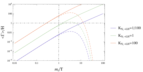
Refer to caption
Refer to caption
Figure 18: The left plot shows the thermal equilibrium parameter 𝒦NiLHsubscript𝒦subscript𝑁𝑖𝐿𝐻\mathcal{K}_{N_{i}\leftrightarrow LH} for both decays (plain) and inverse decays (dashed), for several equilibrium parameters KNiLHsubscript𝐾subscript𝑁𝑖𝐿𝐻K_{N_{i}\leftrightarrow LH}. The right plot shows the solution zdsubscript𝑧𝑑z_{d} and zid±superscriptsubscript𝑧𝑖𝑑plus-or-minusz_{id}^{\pm} to the equilibrium condition for decays and inverse decays respectively. Decays and inverse decays are both in equilibrium in the gray area, which only happens if K0.6𝐾0.6K\geq 0.6.

In order to be specific, we will consider how these formulae apply to the case of leptonic RHN decays and inverse decays, NiLHsubscript𝑁𝑖𝐿𝐻N_{i}\leftrightarrow LH, directly relevant for leptogenesis. In equilibrium, we have

Yieq=nieqnγeq=38zi2K2(zi),YLeq=34.formulae-sequencesubscriptsuperscript𝑌𝑒𝑞𝑖superscriptsubscript𝑛𝑖𝑒𝑞subscriptsuperscript𝑛𝑒𝑞𝛾38superscriptsubscript𝑧𝑖2subscript𝐾2subscript𝑧𝑖subscriptsuperscript𝑌𝑒𝑞𝐿34Y^{eq}_{i}=\frac{n_{i}^{eq}}{n^{eq}_{\gamma}}=\frac{3}{8}z_{i}^{2}K_{2}(z_{i}),\quad Y^{eq}_{L}=\frac{3}{4}. (99)

Note that the derivation of the Boltzmann equations in the form (95) assumed Maxwell-Boltzmann statistics for all the particles. This assumption should technically lead to Yieq=zi2K2(zi)/2subscriptsuperscript𝑌𝑒𝑞𝑖superscriptsubscript𝑧𝑖2subscript𝐾2subscript𝑧𝑖2Y^{eq}_{i}=z_{i}^{2}K_{2}(z_{i})/2. However, we know that relativistic fermions have an abundance YLeq=3/4subscriptsuperscript𝑌𝑒𝑞𝐿34Y^{eq}_{L}=3/4. In order to reproduce the relativistic RHN abundance at TMimuch-greater-than𝑇subscript𝑀𝑖T\gg M_{i}, we multiply by an overall 3/4343/4, so that Yieq(zi0)=3/4subscriptsuperscript𝑌𝑒𝑞𝑖subscript𝑧𝑖034Y^{eq}_{i}(z_{i}\rightarrow 0)=3/4 Hahn-Woernle et al. (2009); Davidson et al. (2008). The thermal equilibrium parameters take the form

𝒦NiLH=KNiLHzi2K1(zi)K2(zi),𝒦LHNi=KNiLHzi2K1(zi)K2(zi)YieqYLeq.formulae-sequencesubscript𝒦subscript𝑁𝑖𝐿𝐻subscript𝐾subscript𝑁𝑖𝐿𝐻superscriptsubscript𝑧𝑖2subscript𝐾1subscript𝑧𝑖subscript𝐾2subscript𝑧𝑖subscript𝒦𝐿𝐻subscript𝑁𝑖subscript𝐾subscript𝑁𝑖𝐿𝐻superscriptsubscript𝑧𝑖2subscript𝐾1subscript𝑧𝑖subscript𝐾2subscript𝑧𝑖subscriptsuperscript𝑌𝑒𝑞𝑖subscriptsuperscript𝑌𝑒𝑞𝐿\begin{split}&\mathcal{K}_{N_{i}\rightarrow LH}=K_{N_{i}\rightarrow LH}z_{i}^{2}\frac{K_{1}(z_{i})}{K_{2}(z_{i})},\\ &\mathcal{K}_{LH\rightarrow N_{i}}=K_{N_{i}\rightarrow LH}z_{i}^{2}\frac{K_{1}(z_{i})}{K_{2}(z_{i})}\frac{Y^{eq}_{i}}{Y^{eq}_{L}}.\end{split} (100)

Of course, it is a matter of convention to use 1/YLeq1subscriptsuperscript𝑌𝑒𝑞𝐿1/Y^{eq}_{L} rather than 1/YHeq1subscriptsuperscript𝑌𝑒𝑞𝐻1/Y^{eq}_{H} in the definition of the thermal equilibrium parameter for inverse decays. These two functions have been plotted in figure 18 for various parameters KNiLHsubscript𝐾subscript𝑁𝑖𝐿𝐻K_{N_{i}\rightarrow LH}. The equilibrium conditions for the decays and inverse decays are given as 𝒦NiLH>1subscript𝒦subscript𝑁𝑖𝐿𝐻1\mathcal{K}_{N_{i}\rightarrow LH}>1 and 𝒦LHNi>1subscript𝒦𝐿𝐻subscript𝑁𝑖1\mathcal{K}_{LH\rightarrow N_{i}}>1 respectively. The first condition translates to a restriction on zi>zdsubscript𝑧𝑖subscript𝑧𝑑z_{i}>z_{d}, while the second translates to the condition zid+>zi>zidsubscriptsuperscript𝑧𝑖𝑑subscript𝑧𝑖subscriptsuperscript𝑧𝑖𝑑z^{+}_{id}>z_{i}>z^{-}_{id}. The solutions zdsubscript𝑧𝑑z_{d}, and zid±subscriptsuperscript𝑧plus-or-minus𝑖𝑑z^{\pm}_{id} have been numerically solved and plotted in Fig. 18.


Appendix C Decay rates and scattering cross sections

This appendix compiles the relevant decay rates and scattering cross sections used in the HPL Boltzmann equations. We summarize the relevant scattering processes in Fig. 19.
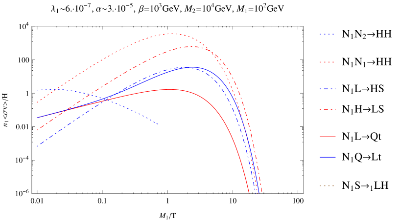
Refer to caption

Figure 19: This plot is a summary of the important scattering processes to account for, in order to properly manage the effect of N1subscript𝑁1N_{1} on the lepton asymmetry. The corresponding Feynman diagrams are shown in the main text, in Fig. 7.

Decays and inverse decays

At tree level, one has the RHN decay rates to leptons,

Γ(NiLH)=Γ(NiLH¯)=k,α,βΓ(NiLkαHβ)=(λλ)ii16πMi,Γi=Γ(NiLH)+Γ(NiLH¯)=(λλ)ii8πMi.formulae-sequenceΓsubscript𝑁𝑖𝐿𝐻Γsubscript𝑁𝑖¯𝐿𝐻subscript𝑘𝛼𝛽Γsubscript𝑁𝑖superscriptsubscript𝐿𝑘𝛼superscript𝐻𝛽subscriptsuperscript𝜆𝜆𝑖𝑖16𝜋subscript𝑀𝑖subscriptΓ𝑖Γsubscript𝑁𝑖𝐿𝐻Γsubscript𝑁𝑖¯𝐿𝐻subscriptsuperscript𝜆𝜆𝑖𝑖8𝜋subscript𝑀𝑖\begin{split}&\Gamma(N_{i}\rightarrow LH)=\Gamma(N_{i}\rightarrow\overline{LH})=\sum_{k,\alpha,\beta}\Gamma(N_{i}\rightarrow L_{k}^{\alpha}H^{\beta})=\frac{(\lambda^{\dagger}\lambda)_{ii}}{16\pi}M_{i},\\ &\Gamma_{i}=\Gamma(N_{i}\rightarrow LH)+\Gamma(N_{i}\rightarrow\overline{LH})=\frac{(\lambda^{\dagger}\lambda)_{ii}}{8\pi}M_{i}.\end{split} (101)

The indices α,β=1,2formulae-sequence𝛼𝛽12\alpha,\beta=1,2 refer to the SU(2) doublets, and enumerate the electron-type and the neutrino-type leptons. The index k=1,2,3𝑘123k=1,2,3 runs through the three families, electron, muon, and tau. One of the hidden sector decays we encounter is N2N1Ssubscript𝑁2subscript𝑁1𝑆N_{2}\rightarrow N_{1}S,

Γ(N2N1S)=|α12|2M216π[(1+M1M2)2mS2M22](1M12M22mS2M22)24M12M22mS2M22,Γsubscript𝑁2subscript𝑁1𝑆superscriptsubscript𝛼122subscript𝑀216𝜋delimited-[]superscript1subscript𝑀1subscript𝑀22superscriptsubscript𝑚𝑆2superscriptsubscript𝑀22superscript1superscriptsubscript𝑀12superscriptsubscript𝑀22superscriptsubscript𝑚𝑆2superscriptsubscript𝑀2224superscriptsubscript𝑀12superscriptsubscript𝑀22superscriptsubscript𝑚𝑆2superscriptsubscript𝑀22\Gamma(N_{2}\rightarrow N_{1}S)=\frac{|\alpha_{12}|^{2}M_{2}}{16\pi}\left[\left(1+\frac{M_{1}}{M_{2}}\right)^{2}-\frac{m_{S}^{2}}{M_{2}^{2}}\right]\sqrt{\left(1-\frac{M_{1}^{2}}{M_{2}^{2}}-\frac{m_{S}^{2}}{M_{2}^{2}}\right)^{2}-4\frac{M_{1}^{2}}{M_{2}^{2}}\frac{m_{S}^{2}}{M_{2}^{2}}}, (102)

where we used the approximation that αij=Re{αij}subscript𝛼𝑖𝑗Resubscript𝛼𝑖𝑗\alpha_{ij}=\text{Re}\{\alpha_{ij}\}, which is not generally true because of the complex phases contained in α𝛼\alpha, but the CP𝐶𝑃CP-odd contributions are not relevant here as the decay is L𝐿L-conserving.

Visible sector scattering

These processes involve the SM quarks and leptons in external states.

  • s𝑠s-channel: the NiLQtsubscript𝑁𝑖𝐿𝑄𝑡N_{i}L\leftrightarrow Qt cross section and reduced cross section read

    σ(NiLQt¯)=α,kσ(NiLkαQt¯)=(λλ)ii8πmt2v21s,σ^(NiLQt¯)=(λλ)ii8πmt2v2(sMi2)2s2.formulae-sequence𝜎subscript𝑁𝑖𝐿𝑄¯𝑡subscript𝛼𝑘𝜎subscript𝑁𝑖superscriptsubscript𝐿𝑘𝛼𝑄¯𝑡subscriptsuperscript𝜆𝜆𝑖𝑖8𝜋superscriptsubscript𝑚𝑡2superscript𝑣21𝑠^𝜎subscript𝑁𝑖𝐿𝑄¯𝑡subscriptsuperscript𝜆𝜆𝑖𝑖8𝜋superscriptsubscript𝑚𝑡2superscript𝑣2superscript𝑠superscriptsubscript𝑀𝑖22superscript𝑠2\begin{split}&\sigma(N_{i}L\rightarrow Q\overline{t})=\sum_{\alpha,k}\sigma(N_{i}L_{k}^{\alpha}\rightarrow Q\overline{t})=\frac{(\lambda^{\dagger}\lambda)_{ii}}{8\pi}\frac{m_{t}^{2}}{v^{2}}\frac{1}{s},\\ &\hat{\sigma}(N_{i}L\rightarrow Q\overline{t})=\frac{(\lambda^{\dagger}\lambda)_{ii}}{8\pi}\frac{m_{t}^{2}}{v^{2}}\frac{(s-M_{i}^{2})^{2}}{s^{2}}.\end{split} (103)
  • t𝑡t-channel: We consider NiQLtsubscript𝑁𝑖𝑄𝐿𝑡N_{i}Q\leftrightarrow Lt and NitLQsubscript𝑁𝑖𝑡𝐿𝑄N_{i}t\leftrightarrow LQ. Because the leptons and quarks are assumed massless, these two channels are in fact equal. We have the cross section and reduced cross sections

    σ(NiQLt)=(λλ)ii8πmt2v21s[s2Mi2+2mh2sMi2+mh2+2Mi2mh2sMi2ln(sMi2+mh2mh2)],σ^(NiQLt)=(λλ)ii8πmt2v2sMi2s[s2Mi2+2mh2sMi2+mh2+2Mi2mh2sMi2ln(sMi2+mh2mh2)].formulae-sequence𝜎subscript𝑁𝑖𝑄𝐿𝑡subscriptsuperscript𝜆𝜆𝑖𝑖8𝜋superscriptsubscript𝑚𝑡2superscript𝑣21𝑠delimited-[]𝑠2superscriptsubscript𝑀𝑖22superscriptsubscript𝑚2𝑠superscriptsubscript𝑀𝑖2superscriptsubscript𝑚22superscriptsubscript𝑀𝑖2superscriptsubscript𝑚2𝑠superscriptsubscript𝑀𝑖2𝑠superscriptsubscript𝑀𝑖2superscriptsubscript𝑚2superscriptsubscript𝑚2^𝜎subscript𝑁𝑖𝑄𝐿𝑡subscriptsuperscript𝜆𝜆𝑖𝑖8𝜋superscriptsubscript𝑚𝑡2superscript𝑣2𝑠superscriptsubscript𝑀𝑖2𝑠delimited-[]𝑠2superscriptsubscript𝑀𝑖22superscriptsubscript𝑚2𝑠superscriptsubscript𝑀𝑖2superscriptsubscript𝑚22superscriptsubscript𝑀𝑖2superscriptsubscript𝑚2𝑠superscriptsubscript𝑀𝑖2𝑠superscriptsubscript𝑀𝑖2superscriptsubscript𝑚2superscriptsubscript𝑚2\begin{split}&\sigma(N_{i}Q\rightarrow Lt)=\frac{(\lambda^{\dagger}\lambda)_{ii}}{8\pi}\frac{m_{t}^{2}}{v^{2}}\frac{1}{s}\left[\frac{s-2M_{i}^{2}+2m_{h}^{2}}{s-M_{i}^{2}+m_{h}^{2}}+2\frac{M_{i}^{2}-m_{h}^{2}}{s-M_{i}^{2}}\ln\left(\frac{s-M_{i}^{2}+m_{h}^{2}}{m_{h}^{2}}\right)\right],\\ &\hat{\sigma}(N_{i}Q\rightarrow Lt)=\frac{(\lambda^{\dagger}\lambda)_{ii}}{8\pi}\frac{m_{t}^{2}}{v^{2}}\frac{s-M_{i}^{2}}{s}\left[\frac{s-2M_{i}^{2}+2m_{h}^{2}}{s-M_{i}^{2}+m_{h}^{2}}+2\frac{M_{i}^{2}-m_{h}^{2}}{s-M_{i}^{2}}\ln\left(\frac{s-M_{i}^{2}+m_{h}^{2}}{m_{h}^{2}}\right)\right].\end{split} (104)

    Throughout this paper, we take the approximation that the zero-temperature Higgs mass mh=0subscript𝑚0m_{h}=0, but in this limit, these cross sections are infrared divergent. The regulator to use, however, is the thermal mass which can potentially be quite large at leptogenesis temperatures. In practice, the cross section is only logarithmically sensitive to the regulator, and we therefore make the conventional choice mh/Mi=105subscript𝑚subscript𝑀𝑖superscript105m_{h}/M_{i}=10^{-5}.

Hidden sector scattering

  • s𝑠s-channel: NiLHSsubscript𝑁𝑖𝐿𝐻𝑆N_{i}L\leftrightarrow HS through the βHHS𝛽𝐻𝐻𝑆\beta HHS vertex. The cross section and reduced cross section are

    σ(NiLHS)=α,kσ(NiLkαHS)=(λλ)iiβ28πsmS2s3,σ^(NiLHS)=(λλ)iiβ28π(smS2)(sMi2)2s4.formulae-sequence𝜎subscript𝑁𝑖𝐿𝐻𝑆subscript𝛼𝑘𝜎subscript𝑁𝑖superscriptsubscript𝐿𝑘𝛼𝐻𝑆subscriptsuperscript𝜆𝜆𝑖𝑖superscript𝛽28𝜋𝑠superscriptsubscript𝑚𝑆2superscript𝑠3^𝜎subscript𝑁𝑖𝐿𝐻𝑆subscriptsuperscript𝜆𝜆𝑖𝑖superscript𝛽28𝜋𝑠superscriptsubscript𝑚𝑆2superscript𝑠superscriptsubscript𝑀𝑖22superscript𝑠4\begin{split}&\sigma(N_{i}L\rightarrow HS)=\sum_{\alpha,k}\sigma(N_{i}L_{k}^{\alpha}\rightarrow HS)=\frac{(\lambda^{\dagger}\lambda)_{ii}\beta^{2}}{8\pi}\frac{s-m_{S}^{2}}{s^{3}},\\ &\hat{\sigma}(N_{i}L\rightarrow HS)=\frac{(\lambda^{\dagger}\lambda)_{ii}\beta^{2}}{8\pi}\frac{(s-m_{S}^{2})(s-M_{i}^{2})^{2}}{s^{4}}.\end{split} (105)
  • s𝑠s-channel: NiSLHsubscript𝑁𝑖𝑆𝐿𝐻N_{i}S\leftrightarrow LH, through the hidden sector vertex αijNiNjSsubscript𝛼𝑖𝑗subscript𝑁𝑖subscript𝑁𝑗𝑆\alpha_{ij}N_{i}N_{j}S. This process is mediated by Njsubscript𝑁𝑗N_{j}, and the amplitude should thus be summed over all flavors. However, we shall simplify the discussion by considering only one internal flavor. In the the limit of massless S𝑆S, the cross section takes the form

    σ(NiSLH)=jα,kσ(NiSLkαH)=j(λλ)jj|αij|216π(s+Mi2)(s+Mj2)4sMiMjδ(s,Mi2,ms2)((sMj2)2+j2),σ^(NiSLH)=j(λλ)jj|αij|216π(sMi2)s(s+Mi2)(s+Mj2)4sMiMj(sMj2)2+j2,j=MjΓj.\begin{split}&\sigma(N_{i}S\rightarrow LH)=\sum_{j}\sum_{\alpha,k}\sigma(N_{i}S\rightarrow L_{k}^{\alpha}H)=\sum_{j}\frac{(\lambda^{\dagger}\lambda)_{jj}|\alpha_{ij}|^{2}}{16\pi}\frac{(s+M_{i}^{2})(s+M_{j}^{2})-4sM_{i}M_{j}}{\sqrt{\delta(s,M_{i}^{2},m_{s}^{2})}((s-M_{j}^{2})^{2}+{\cal E}_{j}^{2})},\\ &\hat{\sigma}(N_{i}S\rightarrow LH)=\sum_{j}\frac{(\lambda^{\dagger}\lambda)_{jj}|\alpha_{ij}|^{2}}{16\pi}\frac{(s-M_{i}^{2})}{s}\frac{(s+M_{i}^{2})(s+M_{j}^{2})-4sM_{i}M_{j}}{(s-M_{j}^{2})^{2}+{\cal E}_{j}^{2}},\qquad{\cal E}_{j}=M_{j}\Gamma_{j}.\end{split} (106)
  • s𝑠s-channel: NiNjHHsubscript𝑁𝑖subscript𝑁𝑗𝐻𝐻N_{i}N_{j}\leftrightarrow HH mediated by S𝑆S. Taking the notation, δ(s,Mi,Mj)=(sMi2Mj2)24Mi2Mj2𝛿𝑠subscript𝑀𝑖subscript𝑀𝑗superscript𝑠superscriptsubscript𝑀𝑖2superscriptsubscript𝑀𝑗224superscriptsubscript𝑀𝑖2superscriptsubscript𝑀𝑗2\delta(s,M_{i},M_{j})=(s-M_{i}^{2}-M_{j}^{2})^{2}-4M_{i}^{2}M_{j}^{2}, the cross section and reduced cross section are given by

    σ(NiNjHH)=|αij|2β232πs(Mi+Mj)2δ(s,Mi,Mj)(smS2)2,σ^(NiNjHH)=|αij|2β232πδ(s,Mi,Mj)s(Mi+Mj)2s(smS2)2.formulae-sequence𝜎subscript𝑁𝑖subscript𝑁𝑗𝐻𝐻superscriptsubscript𝛼𝑖𝑗2superscript𝛽232𝜋𝑠superscriptsubscript𝑀𝑖subscript𝑀𝑗2𝛿𝑠subscript𝑀𝑖subscript𝑀𝑗superscript𝑠superscriptsubscript𝑚𝑆22^𝜎subscript𝑁𝑖subscript𝑁𝑗𝐻𝐻superscriptsubscript𝛼𝑖𝑗2superscript𝛽232𝜋𝛿𝑠subscript𝑀𝑖subscript𝑀𝑗𝑠superscriptsubscript𝑀𝑖subscript𝑀𝑗2𝑠superscript𝑠superscriptsubscript𝑚𝑆22\begin{split}&\sigma(N_{i}N_{j}\rightarrow HH)=\frac{|\alpha_{ij}|^{2}\beta^{2}}{32\pi}\frac{s-(M_{i}+M_{j})^{2}}{\sqrt{\delta(s,M_{i},M_{j})}(s-m_{S}^{2})^{2}},\\ &\hat{\sigma}(N_{i}N_{j}\rightarrow HH)=\frac{|\alpha_{ij}|^{2}\beta^{2}}{32\pi}\sqrt{\delta(s,M_{i},M_{j})}\frac{s-(M_{i}+M_{j})^{2}}{s(s-m_{S}^{2})^{2}}.\end{split} (107)
  • t𝑡t-channel: NiHLSsubscript𝑁𝑖𝐻𝐿𝑆N_{i}H\leftrightarrow LS and NiSLHsubscript𝑁𝑖𝑆𝐿𝐻N_{i}S\leftrightarrow LH, both mediated by a Higgs. Care is needed in computing these cross sections, because the Higgs mediator can be produced on-shell. This is true even if the Higgs has a small but finite mass. Thus, these processes will almost always be divergent, as they include the kinematic regime where the RH neutrino decays on-shell to LH𝐿𝐻LH. It is therefore important to note that the cross section is regulated by the external neutrino decay width. This subtlety has been noted previously in a different context Ginzburg (1995); *Melnikov:1996iu. Starting with NiHLSsubscript𝑁𝑖𝐻𝐿𝑆N_{i}H\rightarrow LS, the amplitude squared takes the form

    α,β,kspins|i(NiHβLkαS)|2=2β2[(λλ)iiMi2t2+i2(λλ)iitt2+i2].subscript𝛼𝛽𝑘subscript𝑠𝑝𝑖𝑛𝑠superscript𝑖subscript𝑁𝑖superscript𝐻𝛽subscriptsuperscript𝐿𝛼𝑘𝑆22superscript𝛽2delimited-[]subscriptsuperscript𝜆𝜆𝑖𝑖superscriptsubscript𝑀𝑖2superscript𝑡2superscriptsubscript𝑖2subscriptsuperscript𝜆𝜆𝑖𝑖𝑡superscript𝑡2superscriptsubscript𝑖2\sum_{\alpha,\beta,k}\sum_{spins}|i\mathcal{M}(N_{i}H^{\beta}\rightarrow L^{\alpha}_{k}S)|^{2}=2\beta^{2}\left[\frac{(\lambda^{\dagger}\lambda)_{ii}M_{i}^{2}}{t^{2}+{\cal E}_{i}^{2}}-(\lambda^{\dagger}\lambda)_{ii}\frac{t}{t^{2}+{\cal E}_{i}^{2}}\right]. (108)

    Upon integration over the transfer momentum, the second term leads to a logarithmic divergence. The first term is naively more problematic because it leads to a linear divergence, 1/i1subscript𝑖1/{\cal E}_{i}. However, in the narrow width limit, upon integration this term gives the delta function δ(t)𝛿𝑡\delta(t). This is the signature of an on-shell mediator, which splits the scattering into the two on-shell subprocesses NLH𝑁𝐿𝐻N\rightarrow LH followed by HHS𝐻𝐻𝑆HH\rightarrow S. The first part is already accounted for in the Boltzmann equations, and should be subtracted in order to avoid double-counting Giudice et al. (2004). In effect, this is a t𝑡t-channel RIS. The subtracted scattering cross section we use is then

    σ(NiHLS)=(λλ)iiβ216π(sMi2)2log(s2(sMi2mS2)2+s2i2Mi4mS4+s2i2),σ^(NiHLS)=(λλ)iiβ216πslog(s2(sMi2mS2)2+s2i2mS4+s2i2),i=MiΓi.\begin{split}&\sigma(N_{i}H\rightarrow LS)=\frac{(\lambda^{\dagger}\lambda)_{ii}\beta^{2}}{16\pi(s-M_{i}^{2})^{2}}\log\left(\frac{s^{2}(s-M_{i}^{2}-m_{S}^{2})^{2}+s^{2}{\cal E}_{i}^{2}}{M_{i}^{4}m_{S}^{4}+s^{2}{\cal E}_{i}^{2}}\right),\\ &\hat{\sigma}(N_{i}H\rightarrow LS)=\frac{(\lambda^{\dagger}\lambda)_{ii}\beta^{2}}{16\pi s}\log\left(\frac{s^{2}(s-M_{i}^{2}-m_{S}^{2})^{2}+s^{2}{\cal E}_{i}^{2}}{m_{S}^{4}+s^{2}{\cal E}_{i}^{2}}\right),\quad{\cal E}_{i}=M_{i}\Gamma_{i}.\end{split} (109)

    The decay rate to account for in isubscript𝑖{\cal E}_{i} is the total rate, that is 1=MiΓ1subscript1subscript𝑀𝑖subscriptΓ1{\cal E}_{1}=M_{i}\Gamma_{1} for N1subscript𝑁1N_{1} but 2=M2(Γ2+Γ21)subscript2subscript𝑀2subscriptΓ2subscriptΓ21{\cal E}_{2}=M_{2}\left(\Gamma_{2}+\Gamma_{21}\right) for N2subscript𝑁2N_{2}. This is model dependent, though we can safely assume that λ2,α2105superscript𝜆2superscript𝛼2superscript105\lambda^{2},\alpha^{2}\leqslant 10^{-5}, which inspires our choice i/Mi2=105subscript𝑖superscriptsubscript𝑀𝑖2superscript105{\cal E}_{i}/M_{i}^{2}=10^{-5}. The cross section is only weakly dependent on the prescription, as the residual divergence is logarithmic.

References