A penalization method for calculating the flow beneath travelling water waves of large amplitude

Abstract

A penalization method for a suitable reformulation of the governing equations as a constrained optimization problem provides accurate numerical simulations for large-amplitude travelling water waves in irrotational flows and in flows with constant vorticity.

1 Introduction

Water flows with a uniform underlying current (possibly absent) are termed irrotational flows, while rotational waves describe the interaction of surface water waves with non-uniform currents. The study of the flow beneath an irrotational two-dimensional surface wave in water with a flat bed is quite well-understood: see [3, 7] for theoretical studies, [2, 12] for numerical simulations and [1, 14] for experimental data. For rotational two-dimensional travelling water waves an existence theory for waves of large amplitude is available [6] and some numerical simulations were performed in the case of constant vorticity flows without stagnation points [10, 11] and in the presence of stagnation points [13]. Constant non-zero vorticity is the hallmark of tidal currents, cf. the discussion in [4], and the absence of stagnation points excludes the possibility of a flow-reversal. These flows represent significant examples of rotational waves and our purpose is to pursue their in-depth study. We present a penalization method that selects from the family of solutions to a reformulation of the governing equations genuine waves. This permits us to provide accurate simulations of the surface water wave but also of the main flow characteristics (fluid velocity components, pressure) beneath it.

2 Preliminaries

In this section we present the governing equations for periodic travelling water waves in a flow of constant vorticity over a flat bed. We briefly discuss the reformulation from [6] that leads, by means of bifurcation theory, to the existence of waves of small and large amplitude.

2.1 Steady two-dimensional water waves

Let us first discuss the governing equations for two-dimensional waves travelling at constant speed and without change of shape at the surface of a layer of water above a flat bed, in a flow of constant vorticity. Two-dimensionality means that the waves propagate in a fixed horizontal direction, say $X$, and the flow presents no variation in the horizontal direction orthogonal to the direction of wave propagation. For this reason, it suffices to analyse a vertical cross-section of the flow, parallel to the direction of wave propagation. To model sea waves of large amplitude the assumptions of inviscid flow in a fluid of constant density are appropriate and the effects of surface tension are negligible – see the discussion in [4]. The assumption of a flat bed $Y=-d$ is also reasonable for a considerable proportion of the Earth’s sea floor. Consequently, the cross-section of the fluid domain is of the form

$$\mathcal{D}(t)=\{(X,Y):X\in\mathbb{R}\text{ and }-d<y<\xi(X-ct)\}\;,$$

where $c>0$ is the wave speed, $d>0$ is the average depth and $\xi$ is the free surface. Setting the density of the water $\rho\equiv 1$, the incompressible Euler equations for the velocity field $(U(X-ct,Y),\,V(X-ct,Y))$ and the pressure $P(X-ct,Y)$ are

$$\left\{\begin{array}[]{l}U_{X}+V_{Y}=0\,,\\ (U-c)U_{X}+VU_{Y}=-P_{X}\,,\\ (U-c)V_{X}+VV_{Y}=-P_{Y}-g\,,\end{array}\right.\quad\text{ in }\mathcal{D}(t)\,,$$ (2.1)

where $g$ is the gravitational constant of acceleration. Since the flow is periodic in the $X$-variable, we may assume that the period is $2\pi$, after performing the rescaling $X\mapsto\frac{L}{2\pi}\,X$ in terms of the actual wavelength $L$. In a frame moving at the (constant) wave speed, obtained by means of the change of variables

$$x=X-ct,\quad Y=y\,,$$

we can restrict our attention to the two-dimensional bounded domain

$$\mathcal{D}=\{(x,y):-\pi<x<\pi\text{ and }-d<y<\eta(x)\}\,,$$

bounded above by the free surface profile

$$S=\{(x,y):-\pi<x<\pi\text{ and }y=\eta(x)\}\,,$$

and below by the flat bed

$$B=\{(x,y):-\pi<x<\pi\text{ and }y=-d\}\,.$$

Since $d$ represents the average depth, the waves oscillate around the flat free surface $y=0$, that is

$$\int_{-\pi}^{\pi}\eta(x)\,dx=0,$$

where $\eta(x)=\xi(X-ct)$. Setting

$$u(x,y)=U(X-ct,y),\quad v(x,y)=V(X-ct,Y),\quad{\mathfrak{p}}(x,y)=P(X-ct,Y),$$

(2.1) can be written as

$$\left\{\begin{array}[]{l}u_{x}+v_{y}=0,\\ (u-c)u_{x}+vu_{y}=-{\mathfrak{p}}_{x},\\ (u-c)v_{x}+vv_{y}=-{\mathfrak{p}}_{y}-g\,,\end{array}\right.\quad\text{ in }\mathcal{D}\,.$$ (2.2)

The boundary conditions that select from the solutions to (2.2) those that represent water waves read as follows

$$\left\{\begin{array}[]{l}{\mathfrak{p}}=P_{atm}\text{ on }S,\\ v=(u-c)\eta_{x}\text{ on }S,\\ v=0\text{ on }B\,,\end{array}\right.$$ (2.3)

where $P_{atm}$ is the constant atmospheric pressure. The first condition reflects the fact that surface tension effects are negligible and permits the decoupling of the water motion from the air flow above it, while the second and third condition express the fact that the free surface and the flat bed are interfaces, with no flow possible across them – see the discussion in [4].

An essential flow characteristic is the vorticity $\gamma=v_{x}-u_{y}$, which is indicative of underlying currents. Vanishing vorticity is the hallmark of uniform currents and a constant vorticity characterizes the linearly sheared tidal currents. With respect to the flow beneath the waves, we restrict our attention to flows for which

$$u<c\quad\hbox{throughout the fluid}.$$ (2.4)

This condition prevents the appearance of stagnation points in the flow and the occurrence of flow-reversals.

2.2 Stream function formulation

Structural properties of the governing equations (2.2)-(2.3) enable us to reduce the number of unknowns. We first introduce the relative mass flux

$$p_{0}=\int_{-d}^{\eta(x)}\big{(}u(x,y)-c\big{)}\,dy<0,$$ (2.5)

since the first equation in (2.2) and the last two equations in (2.3) show that $\int\limits_{-d}^{\eta(x)}\big{(}u(x,y)-c\big{)}\,dy$ is independent of $x$, while (2.4) determines the sign. The first equation in (2.2) permits us to introduce the stream function $\psi(x,y)$ as the unique solution of the differential equations

$$\psi_{x}=-v,\qquad\psi_{y}=u-c\text{ in }\ \overline{\mathcal{D}}\,,$$ (2.6)

subject to

$$\psi(x,-d)=-p_{0}\;.$$ (2.7)

Note that $\psi(x,y)$ is periodic in the $x$-variable, and that the third equation in (2.3) is consistent with the constraint (2.7). Moreover, (2.6) and the definition of vorticity yield

$$\Delta\psi=-\omega\ \text{in }\ \mathcal{D}\;.$$ (2.8)

The first equation in (2.3) is equivalent to $\psi$ being constant on $S$, while (2.5) together with (2.7) ensure that this constant must vanish, that is,

$$\psi=0\ \text{ on }\ \mathcal{S}\;.$$ (2.9)

On the other hand, due to (2.6), we see that we can re-express the Euler equation in (2.2) by the fact that the expression $\frac{(u-c)^{2}+v^{2}}{2}+gy+{\mathfrak{p}}+\gamma\psi$ equals a constant $E$ throughout $\mathcal{D}$. The constant $Q=E-P_{atm}$ is called the hydraulic head.

The previous considerations show that the governing equations (2.2)-(2.3) can be reformulated in terms of the stream function as the free-boundary problem

$$\left\{\begin{array}[]{l}\Delta\psi=-\omega\quad\text{in}\quad{\mathcal{D}}\,,\\ \psi=0\quad\hbox{on}\quad S\,,\\ \psi=p_{0}\quad\hbox{on}\quad B\,,\\ \frac{|\nabla\psi|^{2}}{2}+gy=Q\quad\hbox{on}\quad S\,.\end{array}\right.$$ (2.10)

Given $p_{0}$, we seek values of $d$ and $Q$ for which (2.10) admits a smooth solution $\psi(x,y)$, even and of period $2\pi$ in the $x$-variable. Evenness reflects the requirement that $u$ and $\eta$ are symmetric while $v$ is antisymmetric about the crest line $x=0$; here, we shift the moving frame to ensure that the wave crest is located at $x=0$. Symmetric waves present these features and it is known that a solution with a free surface $S$ that is monotone between crest and trough has to be symmetric, cf. [5].

2.3 Hodograph transform

Under the assumption (2.4), a partial hodograph transform leads to a reformulation of the free-boundary problem (2.10) as a quasilinear elliptic system in a known strip. In this process, the wavelength is normalized to $2\pi$ and the gravitational constant $g$, the relative mass flux $p_{0}$ and the constant vorticity $\gamma$ are considered to be known, while the average depth $d$ and the hydraulic head $Q$ are allowed to vary to accommodate the existence of a flow.

The assumption (2.4) and the definition of the stream function (2.6) yield that $\psi(x,y)$ is a strictly decreasing function of $y$ throughout the fluid domain ${\mathcal{D}}$, being periodic in the $x$-variable. Moreover, due to (2.7) and (2.9), $\psi$ is constant both on the bottom $B$ and on the free surface $S$. The Dubreil-Jacotin transformation [9]

$$q=x,\qquad p=-\psi,$$

transforms the unknown domain $\mathcal{D}$ to the rectangle

$$R=\{(q,p):\ -\pi<q<\pi\,,\ p_{0}<p<0\}\;,$$ (2.11)

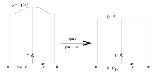
Figure 1: Dubreil-Jacotin transformation

(see Figure 1). Let

$$h(q,p)=y+d$$ (2.12)

define the height above the flat bottom $B$. Since $\psi$ is a strictly decreasing function of $y$, for every fixed $x$ the height $h$ above the flat bottom is a single valued function of $\psi$ (or, equivalently, $p$), with

$$\left\{\begin{array}[]{ccccc}h_{q}&=&\dfrac{v}{u-c},\quad h_{p}&=&\dfrac{1}{c-u}\,,\\[9.38945pt] v&=&-\dfrac{h_{q}}{h_{p}},\quad u&=&c-\dfrac{1}{h_{p}}\,,\end{array}\right.$$

and, more generally,

$$\left\{\begin{array}[]{ccccc}\partial_{x}&=&\partial_{q}-\dfrac{h_{q}}{h_{p}}\,\partial_{p}\,,\quad\partial_{y}&=&\dfrac{1}{h_{p}}\,\partial_{p}\,,\\[5.69046pt] \partial_{p}&=&\dfrac{1}{c-u}\partial_{y}\,,\quad\partial_{q}&=&\partial_{x}-\dfrac{v}{c-u}\partial_{y}\;.\end{array}\right.$$ (2.13)

Using the change of variables relations (2.13), we get that

$$\gamma =\partial_{x}v-\partial_{y}u=\left(\partial_{q}-\frac{h_{q}}{h_{p}}\partial_{p}\right)\left(-\frac{h_{q}}{h_{p}}\right)-\frac{1}{h_{p}}\partial_{p}\left(c-\frac{1}{h_{p}}\right)$$

$$=\dfrac{-h_{p}h_{qq}+h_{q}h_{pq}}{h_{p}^{2}}-\dfrac{-h_{p}h_{q}h_{pq}+h_{q}^{2}h_{pp}}{h_{p}^{3}}-\dfrac{h_{pp}}{h_{p}^{3}},$$

while

$$|\nabla\psi|^{2}=v^{2}+(u-c)^{2}=\dfrac{1+h_{q}^{2}}{h_{p}^{2}}\,.$$

These considerations show that the constitutive equations for the height function $h(q,p)$, which is even and $2\pi$-periodic in $q$, are

$$\left\{\begin{array}[]{l}\mathcal{H}[h]:=(1+h_{q}^{2})h_{pp}-2h_{p}h_{q}h_{pq}+h_{p}^{2}h_{qq}+\gamma h_{p}^{3}=0\ \text{ on }\ R\,,\\ \mathcal{B}_{0}[h]:=1+h_{q}^{2}(q,0)+(2gh-Q)h_{p}^{2}(q,0)=0\,,\\ \mathcal{B}_{1}[h]:=h(q,p_{0})=0\,.\end{array}\right.$$ (2.14)

In the new formulation (2.14), the wave profile $\eta(x)$ is given by $h(q,0)$, the wave height being the difference

$$\max_{q\in[-\pi,\pi]}h(q,0)-\min_{q\in[-\pi,\pi]}h(q,0).$$ (2.15)

while half of (2.15) represents the wave amplitude.

3 Laminar Flow and Linearised Equations

The simplest solutions are the laminar flows with a flat free surface. Near such flows a linearization procedure permits us to obtain the first-order approximations of genuine water waves. These linear waves capture well the characteristics of waves of small amplitude.

3.1 Laminar flows

Let us discuss the solutions describing parallel shear flows, with $\eta\equiv 0$. In this case the solution $h$ of (2.14) is independent of $q$: $h(q,p)=H(p)$ with

$$\left\{\begin{array}[]{l}\mathcal{H}_{L}[H]:=H_{pp}+\gamma H_{p}^{3}=0\text{ in }R\,,\\ \mathcal{B}_{L,0}[H]:=1+(2gH(0)-Q)H_{p}^{2}(0)=0\,,\\ \mathcal{B}_{L,1}[H]:=H(p_{0})=0\;.\end{array}\right.$$ (3.1)

The explicit solution of (3.1) is given by

$$H(p;\lambda)=\frac{2(p-p_{0})}{\sqrt{\lambda+2\gamma p}+\sqrt{\lambda+2\gamma p_{0}}}\,,\quad p_{0}\leq p\leq 0\,,$$ (3.2)

provided that the parameter $\lambda>0$ satisfies the equation

$$Q=\lambda+\frac{4g|p_{0}|}{\sqrt{\lambda}+\sqrt{\lambda+2\gamma p_{0}}}\,.$$ (3.3)

3.2 Linearised Solutions

We now present the outcome of the linearization of the system (2.14) near the laminar flow $H$.

We consider a parametrized family of functions of the form

$$\hat{h}(q,p)=H(p)+bm(q,p)\,,$$ (3.4)

where $b\in\mathbb{R}$ and the function $m$ is even and $2\pi$-periodic in $q$, such that

$$\mathcal{H}[\hat{h}](p,q)=\mathcal{O}(b^{2})\,,\;\mathcal{B}_{0}[\hat{h}](q)=\mathcal{O}(b^{2})\text{ and }\mathcal{B}_{1}[\hat{h}](q)=0\;.$$ (3.5)

Taking the definition of $\mathcal{H},\mathcal{B}_{0},\mathcal{B}_{1}$ from (2.14) into account, we find that $\mathcal{H}[\hat{h}](p,q)$ is given by

$$(1+H_{q}^{2}(p)+2bH_{q}(p)m_{q}(q,p)+b^{2}m_{q}(q,p))(H_{pp}(p)+bm_{pp}(p,q))$$

$$-2(H_{p}(p)+bm_{p}(q,p))(H_{q}(p)+bm_{q}(q,p))(H_{pq}(p)+bm_{pq}(q,p))$$

$$+(H_{p}^{2}(p)+2bH_{p}(p)m_{p}(p,q)+b^{2}m_{p}^{2}(p,q))(H_{qq}(p)+bm_{qq}(p,q))$$

$$+\gamma(H_{p}^{3}(p)+3bm_{p}(p,q)H_{p}(p)+\mathcal{O}(b^{2}))\;.$$

Using the fact that $H_{q}=0$, the expression for $\mathcal{H}[\hat{h}](p,q)$ simplifies to

$$(1+b^{2}m_{q}(q,p))(H_{pp}(p)+bm_{pp}(p,q))$$

$$-2b^{2}(H_{p}(p)+bm_{p}(q,p)m_{q}(q,p)m_{pq}(q,p)$$

$$+b(H_{p}^{2}(p)+2bH_{p}(p)m_{p}(p,q)+b^{2}m_{p}^{2}(p,q))m_{qq}(p,q)$$

$$+\gamma(H_{p}^{3}(p)+3bm_{p}(p,q)H_{p}^{2}(p)+\mathcal{O}(b^{2}))$$

$$=H_{pp}(p)+\gamma H_{p}^{3}(p)$$

$$+b(m_{pp}(p,q)+H_{p}^{2}(p)m_{qq}(p,q)+3\gamma m_{p}(p,q)H_{p}^{2}(p))+\mathcal{O}(b^{2})\;.$$

Similarly,

$$\mathcal{B}_{0}[\hat{h}](q)=1+(2gH(0)-Q)H_{p}^{2}(0)$$

$$+b2H_{p}(0)\left((2gH(0)-Q)m_{p}(q,0)+gH_{p}(0)m(q,0)\right)+\mathcal{O}(b^{2})\;.$$

Using the fact that (3.1) and (3.2) yield $H_{p}(0)=\frac{1}{\sqrt{\lambda}}$ and $2gH(0)-Q=-\lambda$, we infer that

$$\mathcal{B}_{0}[\hat{h}](q)=1+(2gH(0)-Q)H_{p}^{2}(0)$$

$$+b\frac{2}{\lambda}\left(-\lambda^{3/2}m_{p}(q,0)+gm(q,0)\right)+\mathcal{O}(b^{2})\;.$$

$H$ being a solution to (3.1) shows that $\hat{h}$ solves (3.5) if and only if $m$ satisfies the linearised system

$$\left\{\begin{array}[]{l}m_{pp}+H_{p}^{2}m_{qq}=-3\gamma H_{p}^{2}m_{p}\text{ in }R\,,\\ gm(q,0)=\lambda^{3/2}m_{p}(q,0)\text{ for }-\pi<q<\pi\,,\\ m(q,p_{0})=0\text{ for }-\pi<q<\pi\;.\end{array}\right.$$ (3.6)

For a general value of $\lambda>0$, the problem (3.6) will admit only the trivial solution $m\equiv 0$. However, specific values of $\lambda$ produce non-trivial solutions:

• In the irrotational case $\gamma\equiv 0$ we have that the solution to (3.1) is

  $$H(p;\lambda)=\dfrac{p-p_{0}}{\sqrt{\lambda}}\,,$$ (3.7)

  and the non-trivial solution of the linearized equations (3.6) is given by $m(q,p)=M(p)\,\cos(q)$ with

  $$M(p)=\sinh\left(\dfrac{p-p_{0}}{\sqrt{\lambda^{*}}}\right),$$ (3.8)

  where $\lambda^{*}>0$ satisfies the dispersion relation

  $$\lambda+g\tanh\left(\dfrac{p_{0}}{\sqrt{\lambda}}\right)=0\,,$$ (3.9)

  the corresponding value of $Q$ being

  $$Q^{*}=\lambda^{*}-\dfrac{2gp_{0}}{\sqrt{\lambda^{*}}}\;.$$

  We obtain the linear solution

  $$h^{*}(q,p;b)=\dfrac{p-p_{0}}{\sqrt{\lambda^{*}}}+b\cos q\ \sinh\left(\dfrac{p-p_{0}}{\sqrt{\lambda^{*}}}\right),$$ (3.10)

  with $b$ constant. This is the first-order approximation to the solution of the problem (2.14), up to order $\mathcal{O}(b^{2})$, for small enough $b$.

• Similarly, in the case of constant non-zero vorticity $\gamma$, for

  $$Q^{*}=\lambda^{*}-\dfrac{4gp_{0}}{\sqrt{\lambda^{*}}+\sqrt{\lambda^{*}+2p_{0}\gamma}}$$

  we get the linear solution

  $$h^{*}(q,p;b)=H^{*}(p)+b\cos q\ M(p),$$ (3.11)

  with

  $$H^{*}(p)=\frac{2(p-p_{0})}{\sqrt{\lambda^{*}+2\gamma p}+\sqrt{\lambda^{*}+2\gamma p_{0}}}$$ (3.12)

  and

  $$M(p)=\dfrac{1}{\sqrt{\lambda^{*}+2p\gamma}}\sinh\left(\frac{2(p-p_{0})}{\sqrt{\lambda^{*}+2\gamma p}+\sqrt{\lambda^{*}+2\gamma p_{0}}}\right),$$ (3.13)

  where $\lambda^{*}>0$ is the solution of the dispersion relation

  $$\dfrac{\lambda}{g+\gamma\sqrt{\lambda}}+\tanh\left(\dfrac{2p_{0}}{\sqrt{\lambda}+\sqrt{\lambda+2p_{0}\gamma}}\right)=0.$$ (3.14)

3.3 Bifurcation

The interpretation of the previous results in the space of solutions is provided by means of bifurcation theory: near the laminar flows (3.2), as the parameter $\lambda$ varies, there are generally no genuine waves, except at critical values $\lambda=\lambda^{\ast}$ determined by the dispersion relation (3.14). Note that by (3.2) and (2.13), we have that $\sqrt{\lambda}=\frac{1}{H_{p}(0;\lambda)}=c-u(0,0)$, so that this result means that only critical values of the horizontal fluid velocity of the laminar flows at their flat free surface may trigger the appearance of waves. Near this bifurcating laminar flow $H^{\ast}$, we have two solution curves: one laminar solution curve $\lambda\mapsto H(p;\lambda)$, where $\lambda$ and $Q$ are related by (3.3), and one non-laminar solution curve $Q\mapsto h(q,p;Q)$ such that $h_{q}\not\equiv 0$ unless $h=H^{\ast}$. In [6] it was shown that non-laminar solution curve can be extended to a global continuum $\mathcal{C}$ that contains solutions of (2.14) with $\frac{1}{h_{p}(q_{0},p_{0})}\to 0$ at some $(q_{0},p_{0})$. This condition is characteristic of flows such that their horizontal velocity $u$ is arbitrarily close to the speed $c$ of the reference frame, at some point in the fluid, the limiting configuration being a flow with stagnation points.

4 Optimization

In the following, we consider the numerical solution of the free boundary value problem for water waves with constant vorticity.

We propose a Penalization Method (PM) for solving the constraint optimization problem, to minimize

$$\mathcal{E}[h]:=-\int_{R}h_{q}^{2}\,,$$ (4.1)

subject to the PDE constraint that $h$ satisfies (2.14).

The energy function $\mathcal{E}$ is chosen in such a way that it vanishes for laminar flows (in which $h_{q}\equiv 0$), thus selecting genuine waves.

We propose the following implementation the PM method:

1. Initialize $k=0$: Choose a constant $\nu_{0}>0$ (typically small). Find an initial guess $h^{(0)}$ of the solution of (2.14). For initializing $h^{(0)}$ we select $h^{(0)}(q,p)=h^{*}(q,p;b)$ which gets the particular forms (3.10) and (3.11), for $\gamma=0$ and $\gamma\neq 0$, respectively. These forms guarantee that (3.5) holds.

   In order to calculate waves of large amplitude (one branch of the bifurcation is the laminar flow, and the other branch is the one with high amplitude), the particular choice of $b$ is important for initialization: On the one hand the closer $b$ is to $0$, the smaller the residual is (cf. (3.5) ). On the other hand for $b=0$, $h^{*}(q,p;0)$ is a laminar flow, and the PM algorithm is attracted to the laminar flow solution.

2. $k\to k+1$: Given $h^{(k)}$ we solve the following linear equation for $h$, obtained by freezing the coefficients of lower order from the previous iteration step

   $$0= \mathcal{H}_{l}[h^{(k)}](h)$$ (4.2)

   $$= (1+(h_{q}^{(k)})^{2})h_{pp}-2h_{p}^{(k)}h_{q}^{(k)}h_{pq}+(h_{p}^{(k)})^{2}h_{qq}+\gamma\ (h_{p}^{(k)})^{3}$$

   $$\qquad\text{ in }R,$$

   $$0= \mathcal{B}_{l,1}[h^{(k)}](h)$$

   $$= 1+(h_{q}^{(k)})^{2}+(2gh-Q)(h_{p}^{(k)})^{2}\text{ for }p=0,$$

   $$0= \mathcal{B}_{l,2}[h^{(k)}](h)=h\text{ for }p=p_{0}\;.$$

   The solution is denoted by $h^{(k+1)}$.

3. Compute $h_{p}^{(k+1)}$. Because we work with a semi implicit scheme we have to use a relative small step-size, which is determined here.

   • If $h_{p}^{(k+1)}>0$ then put $\nu_{k+1}=\nu_{k}$ and update $h^{(k+2)}(q,p)=h^{(k+1)}(q,p)+\nu_{k+1}h^{(k+1)}_{qq}(q,p).$ We emphasize that $h^{(k+1)}_{qq}$ is the steepest descent energy of the quadratic functional $\mathcal{E}$. From this perspective we might call this algorithm a steepest descent algorithm.

   • else put $\nu_{k+1}=0$ and update

     $$h^{(k+2)}(q,p)=F(p)-h^{(k)}(q,p).$$

     The function $F$ is given by $F(p)\simeq 2\frac{d}{d^{*}}H^{*}(p)$ with $d^{*}$ and $d$ being the depths of $H^{*}(p)$ and $h^{(k)}(q,p)$, respectively. Using (2.12) we see that the depth $d$ of a flow $h(q,p)$ can be computed by

     $$d=\int_{-\pi}^{\pi}h(q,0)dq.$$

4. Stopping criteria: The algorithm is terminated when the system of equations (2.14) is satisfied up to small error, i.e.,

   • $||\mathcal{H}_{l}[h^{(k)}](h^{(k)})||<\epsilon_{1}$ and $||\mathcal{B}_{l,1}[h^{(k)}](h^{(k)})||<\epsilon_{2}$

   and

   • $||h^{(k)}-h^{(k-1)}||<\epsilon_{3}$, or

   • $0<1/h^{(k)}_{p}<\epsilon_{4}$, which means that we are close to a stagnation point, i.e. $c-u=1/h_{p}$ is positive and close to zero.

   If the algorithm is not terminated then move to the second step.

The different branches of the third step guarantee that the residuals of the boundary conditions and the differential equations are decreasing. We have illustrated this for one example in Figure 2, where the necessity of changing the iteration becomes evident. More precisely, for the above algorithm, there is an iteration $m$ that the condition $h_{p}^{(m+1)}>0$ fails and we make the update $h^{(m+2)}(q,p)=F(p)-h^{(m)}(q,p)$.

The simulations show that for all $k=1,\ldots,m$

$$||\mathcal{H}_{l}[h^{(k)}](h^{(k)})||<||\mathcal{H}_{l}[h^{(k-1)}](h^{(k-1)})||$$

and

$$||\mathcal{B}_{l,1}[h^{(k)}](h^{(k)})||>||\mathcal{B}_{l,1}[h^{(k-1)}](h^{(k-1)})||,$$

as this is also depicted in Figure 2. For $k\geq m+2$ we find that

$$||\mathcal{H}_{l}[h^{(k+1)}](h^{(k+1)})||<||\mathcal{H}_{l}[h^{(k)}](h^{(k)})||$$

and

$$||\mathcal{B}_{l,1}[h^{(k+1)}](h^{(k+1)})||<||\mathcal{B}_{l,1}[h^{(k)}](h^{(k)})||,$$

as depicted in Figure 2.

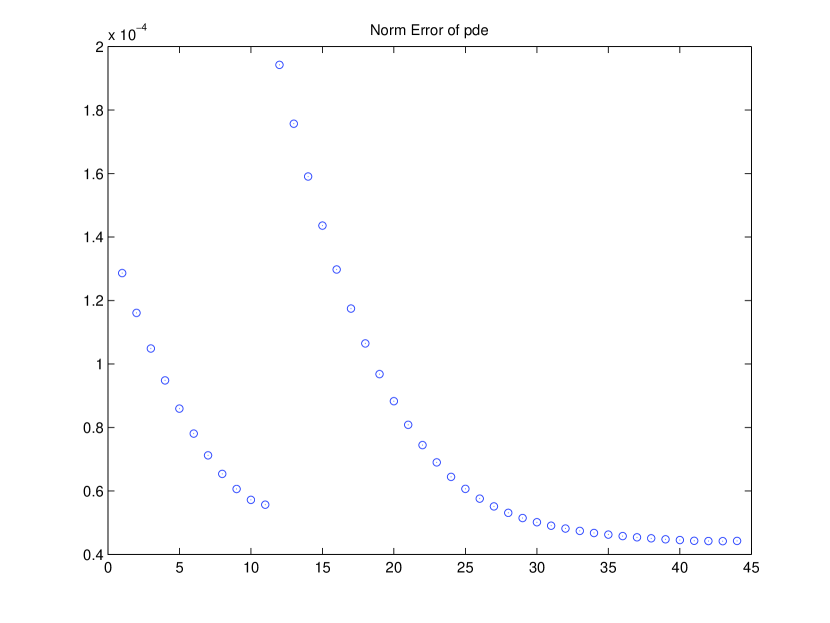
(a) The error of the PDE.

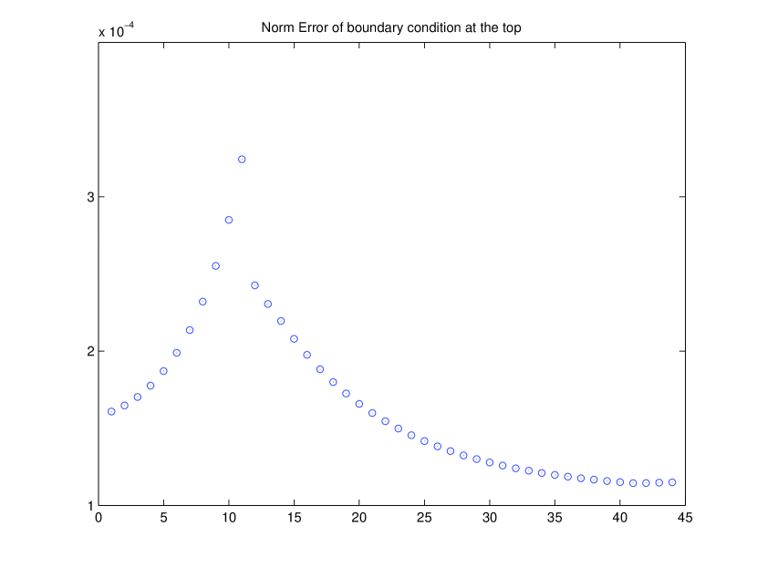
(b) The error of the Boundary condition.

Figure 2: The $L_{2}$ norms of the errors for each iteration.

5 Results

We use that the gravitational constant $g=9.8$ and we fix the relative mass flux $p_{0}=-2$. We present the results of the numerical simulations for three different cases:

• the irrotational case, $\gamma=0$,

• the case of positive vorticity $\gamma=2.95$,

• the case of negative vorticity $\gamma=-1$.

For all the cases we present the figures of

• the profile of the water wave, that is the free boundary $S$,

• the streamline pattern beneath the wave, that is the height $h(q,p)$ along the streamlines $p=-\psi$.

• the distribution of the vertical velocity $v$ in the whole fluid.

• the horizontal velocity $c-u$ on the vertical line below the crest, that is on the straight line segment $\{(q,p):\ q=0,\ p\in[p_{0},0]\}$.

• the distribution of the pressure beneath the wave.

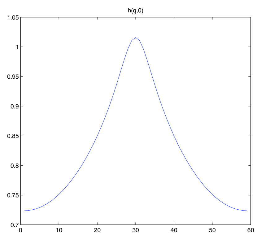
(a) $\gamma=0$

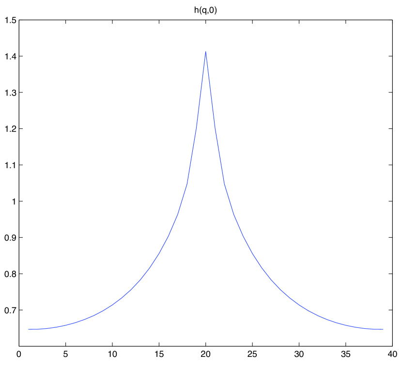
(b) $\gamma=2.95$

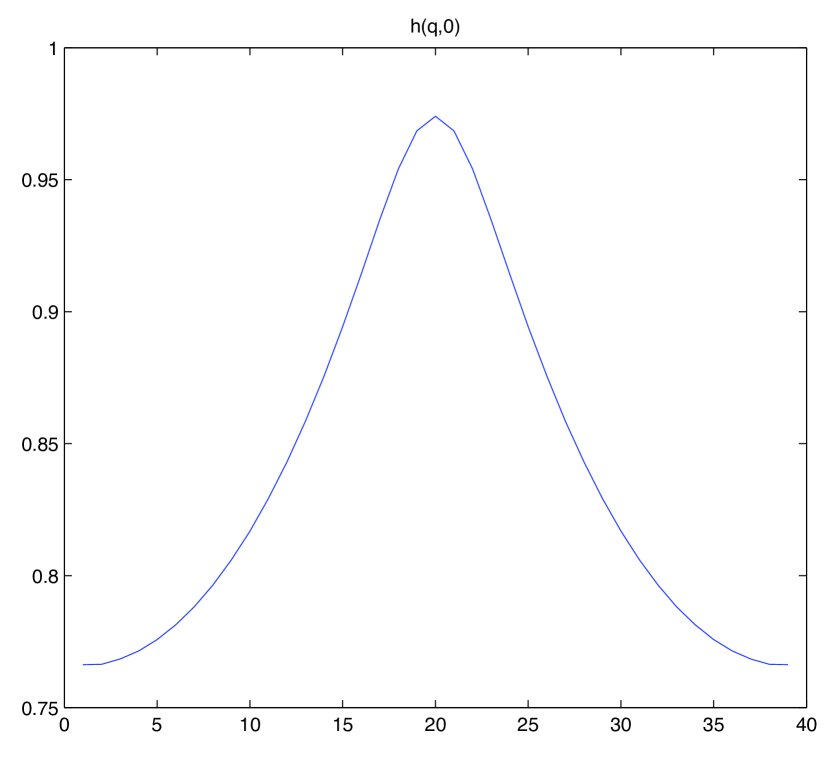
(c) $\gamma=-1$

Figure 3: The periodic wave profile $S$.

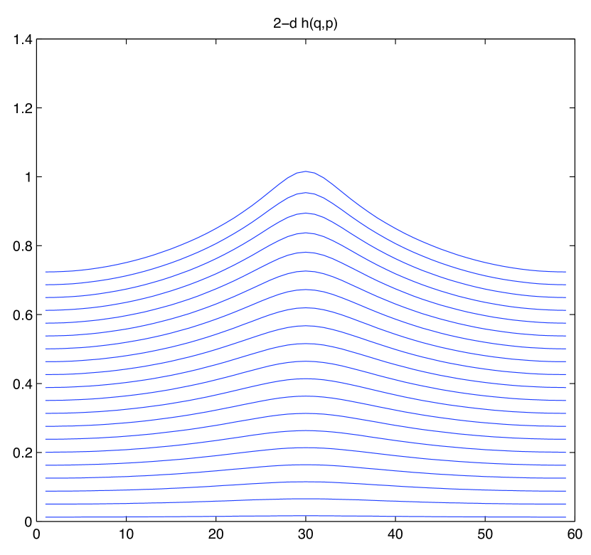
(a) $h(q,p)$

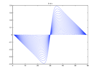
(b) $v(q,p)$

Figure 4: The height $h(q,p)$ of the streamlines and the vertical fluid velocity $v(q,p)$ along streamlines, depicted for the irrotational case $\gamma=0$.

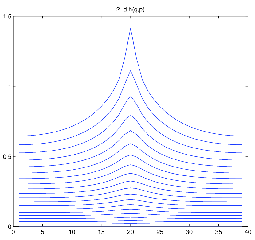
(a) $h(q,p)$

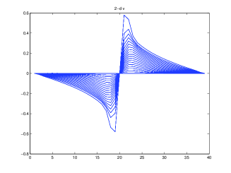
(b) $v(q,p)$

Figure 5: The height $h(q,p)$ of the streamlines and the vertical fluid velocity $v(q,p)$ along streamlines, depicted for the case $\gamma=2.95$.

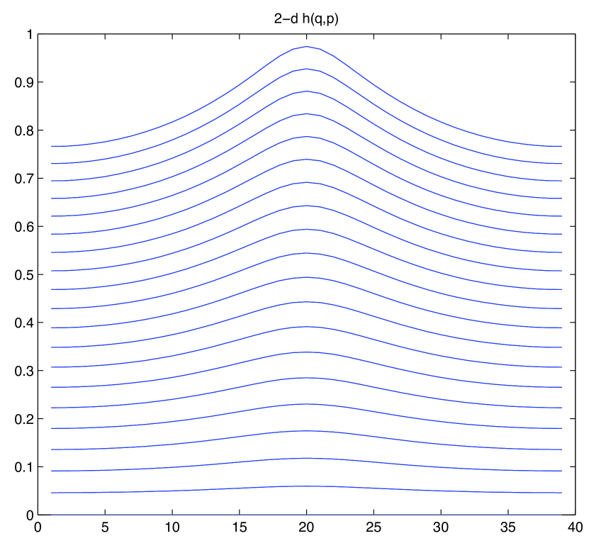
(a) $h(q,p)$

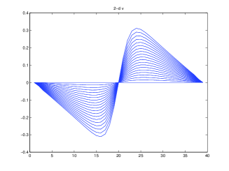
(b) $v(q,p)$

Figure 6: The height $h(q,p)$ of the streamlines and the vertical fluid velocity $v(q,p)$ along streamlines, depicted for the case $\gamma=-1$.

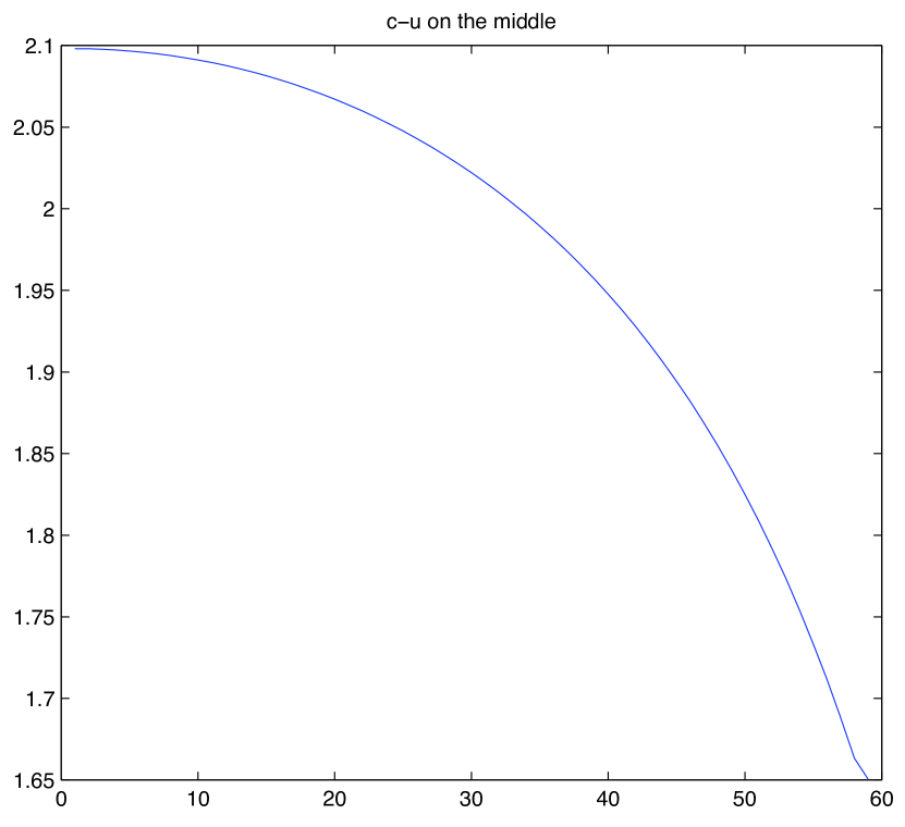
(a) $\gamma=0$

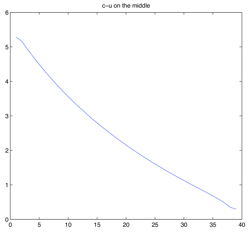
(b) $\gamma=2.95$

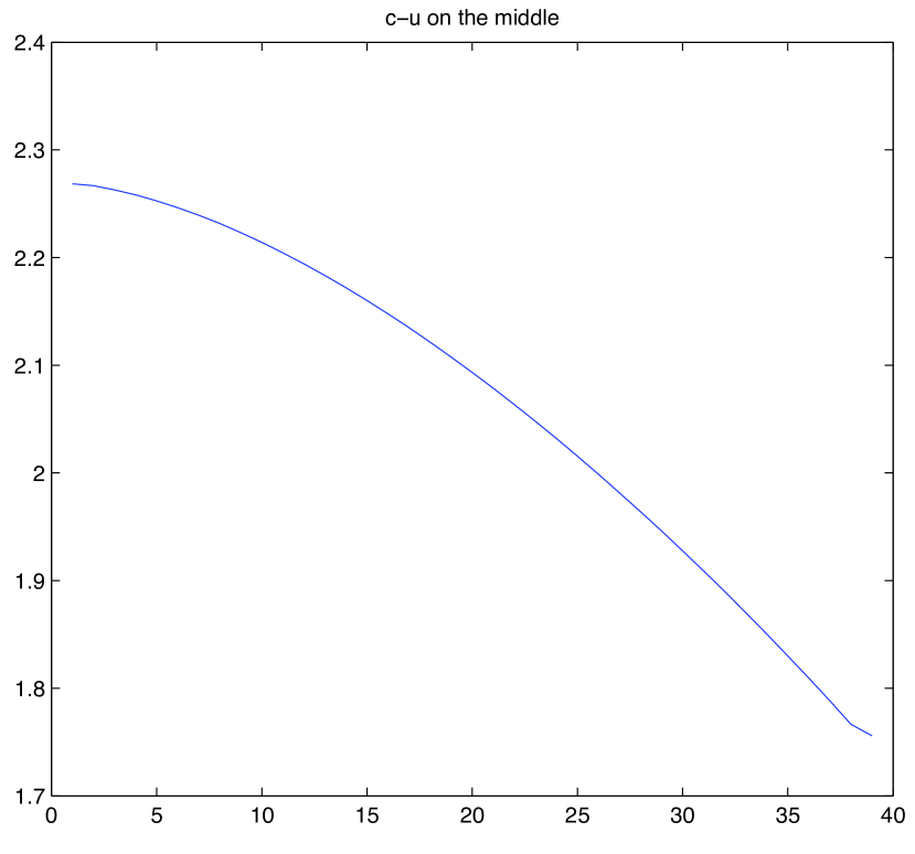
(c) $\gamma=-1$

Figure 7: The horizontal fluid velocity $c-u$ beneath the wave crest, on the line segment $q=0$.

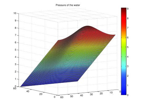
Figure 8: The pressure beneath the wave for $\gamma=0$. The figure depicts the deviation of the pressure from the (constant) atmospheric pressure, ${\mathfrak{p}}-P_{atm}$: vanishing at the free surface $p=0$, it increases as we descend towards the flat bed $p=p_{0}$, the maximum being attained on the bed just below the wave crest (located in the middle of the horizontal segment for the discretization we have made).

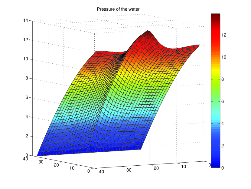
(a) $\gamma=2.95$

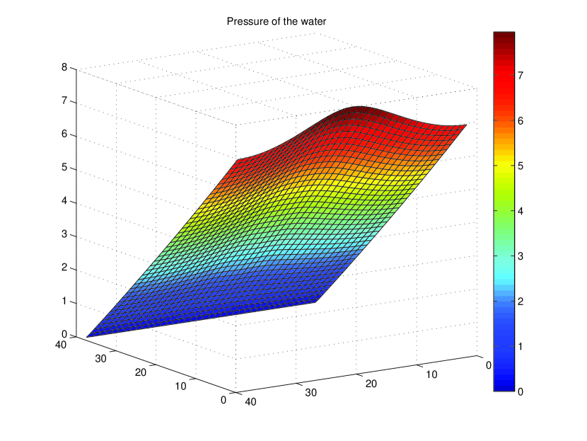
(b) $\gamma=-1$

Figure 9: The pressure beneath rotational water waves.

6 Conclusion

In the present paper we analysed a penalization method for computing two-dimensional travelling water waves. We provided an iterative algorithm that starts with an approximation of a solution of the system (2.14) and converges to a solution which correspond to a water wave of large amplitude. The formula of the initial approximation is given by (3.11) for the non-zero vorticity case; the irrotational case is given as a special case by simply substituting $\gamma=0$.

Moreover, our pursuit for a better approximation of a non-laminar solution (which would serve the initial step of our iterative algorithm) has lead to novel analytical results. In particular, explicit formulas that approximate non-laminar (large amplitude) travelling water waves with constant vorticity are obtained. The relevant analysis and formulas are to be presented in upcoming work.

References

- [1] Y.-Y. Chen, H.-C. Hsu and G.-Y. Chen, Lagrangian experiment and solution for irrotational finite-amplitude progressive gravity waves at uniform depth, Fluid Dyn. Res. 42 (2010), Art. 045511 (34pp.).
- [2] D. Clamond, Note on the velocity and related fields of steady irrotational two-dimensional surface gravity waves, Philos. Trans. Roy. Soc. London A 370 (2012), 1572–-1586.
- [3] A. Constantin, The trajectories of particles in Stokes waves, Invent. Math. 166 (2006), 523–535.
- [4] A. Constantin, Nonlinear water waves with applications to wave-current interactions and tsunamis, CBMS-NSF Conf. Ser. Appl. Math., Vol. 81, SIAM, Philadelphia, 2011.
- [5] A. Constantin, M. Ehrnström and E. Wahlén, Symmetry of steady periodic gravity water waves with vorticity, Duke Math. J. 140 (2007), 591–603.
- [6] A. Constantin and W. Strauss, Exact steady periodic water waves with vorticity, Comm. Pure Appl. Math. 57 (2004), 481–-527.
- [7] A. Constantin and W. Strauss, Pressure beneath a Stokes wave, Comm. Pure Appl. Math. 53 (2010), 533–557.
- [8] A. F. T. da Silva and D. H. Peregrine, Steep, steady surface waves on water of finite depth with constant vorticity, J. Fluid Mech. 195 (1988), 281–302.
- [9] M.-L. Dubreil-Jacotin, Sur la détermination rigoureuse des ondes permanentes périodiques d’ampleur finie, J. Math. Pures Appl. 13 (1934), 217–291.
- [10] J. Ko and W. Strauss, Effect of vorticity on steady water waves, J. Fluid Mech. 608 (2008), 197–215.
- [11] J. Ko and W. Strauss, Large-amplitude steady rotational water waves, Eur. J. Mech. B Fluids 27 (2008), 96–109.
- [12] A. Nachbin and R. Ribeiro-Junior, A boundary integral formulation for particle trajectories in Stokes waves, Discrete Contin. Dyn. Syst. 34 (2014), 3135–-3153.
- [13] V. Vasan and K. Oliveras, Pressure beneath a traveling wave with constant vorticity, Discrete Contin. Dyn. Syst. 34 (2014), 3219–-3239.
- [14] M. Umeyama, Eulerian-Lagrangian analysis for particle velocities and trajectories in a pure wave motion using particle image velocimetry, Philos. Trans. Roy. Soc. London A 370 (2012), 1687–1702.