Matrix Completion under Interval Uncertainty
Abstract
Matrix completion under interval uncertainty can be cast as matrix completion with element-wise box constraints. We present an efficient alternating-direction parallel coordinate-descent method for the problem. We show that the method outperforms any other known method on a benchmark in image in-painting in terms of signal-to-noise ratio, and that it provides high-quality solutions for an instance of collaborative filtering with 100,198,805 recommendations within 5 minutes.
1 Motivation
Matrix completion is a well-known problem, with applications ranging from image processing to recommender systems. When dimensions of a matrix and some of its elements are known, the goal is to find the unknown elements. Without imposing any further requirements on , there are infinitely many solutions. In many applications, however, the matrix completion that minimizes the rank:
| (1) |
provides the simplest explanation for the data. There is a long history of work on the problem, c.f. [9, 36, 47, 21], with thousands of papers published annually since 2010. We hence cannot provide a complete overview.
Let us note that Fazel [10] suggested to replace the rank, which is the sum of non-zero elements of the spectrum, with the nuclear norm, which is the sum of the spectrum. The minimisation of the nuclear norm can be cast as a semidefinite programming (SDP) problem and approaches based on the nuclear-norm have proven very successful in theory [6] and very popular in practice. [36, 3] study the Singular Value Thresholding (SVT) algorithm. This, however, required the computation of a singular value decomposition (SVD) in each iteration. A number of other approaches, e.g., augmented Lagrangian methods [44], appeared, but those would require a truncated SVD or a number of iterations [15, 22, 37, 45] of the power method. Even considering the recent progress in randomized methods for approximating SVD, [13], the approximation becomes very time-consuming as the dimensions of matrices grow.
A major computational break-through came in the form of the alternating least squares (ALS) algorithms [40, 31]. Initially, the algorithm has been used as a heuristic for finding stationary points of the non-convex problem [40, 31, 27, 2, 12], where a single iteration had complexity , for observations and rank , c.f., p. 60 in [20]. Keshavan et al. [19, 20], however, proved its exponential rate of convergence to the global optimum with high probability, under probabilistic assumptions common in the compressed sensing community. Further, more technical analyses of the convergence to the global optimum have been performed by Jain et al. [17].
Many studies of matrix completion consider the uncertainty, in some form. A number of analyses [19, 20, 17] consider the use of the standard rank-minimisation for the reconstruction of low-rank matrix from , where , , with elements of being bounded i.i.d. random variables, which are sub-Gaussian and have bounded expectation. A number of further analyses [46, 4] considered the use of the standard rank-minimisation for the reconstruction of low-rank matrix from , where are as above and has a small number of non-zero entries. [7] consider some columns being corrupted. Although we are not aware of any studies of matrix completion under interval uncertainty, interval-based uncertainty has been considered in related problems. Alaiz et al. [1] consider the min-max variant of the problem of finding the nearest correlation matrix, i.e., the problem of finding the closest matrix within the set of symmetric positive definite matrices with the unit diagonal to an uncertainty set, with respect to the Frobenius norm. [23] studied interval uncertainty in certain semidefinite programming problems, which can be used to encode the nuclear-norm minimisation.
In contrast, we present an extension of matrix completion toward interval uncertainty, which has applications in image in-painting, collaborative filtering, and beyond. The algorithm we present for solving the problem can be seen as a coordinate-wise version of the ALS algorithm, which does not require the approximation of the spectrum of the matrix. This makes it possible solve complete matrices matrix within minutes on a standard laptop. First, we provide an overview of the possible applications.
1.1 Collaborative Filtering under Uncertainty
Collaborative filtering is a well-established application of matrix completion problems [39], largely thanks to the success of the Netflix Prize. There is a matrix, where each row corresponds to one user and each column corresponds to a product or service. Considering that every user rates only a modest number of products or services, there are only a small number of entries of the matrix known. Our extension is motivated by the fact, that one user may provide two different ratings for one and the same product at two different times, depending on the current mood and other circumstances at the two times. One may hence want to consider an interval instead of a fixed value of the rating, e.g., . Further, when one knows the scale the rating is chosen from, one can consider . Hence, if intervals are known for elements of a matrix indexed by , one may want to solve:
| (2) | ||||
| subject to |
Although numerous extensions of matrix completion problems have been studied, e.g. [26], the use of robustness to interval uncertainty is novel. It can be seen as an extension of robust optimisation [38] to matrix completion.
1.2 Image In-Painting
Further applications can be found in image processing. In in-painting problems, a subset of pixels from an image are given and the goal is to fill in the missing pixels. Rank-constrained matrix completion with equalities, where is the index set of all known pixels, has been used numerous times [6, 16, 25, 11, 22, 15, 45, 45] in this setting. If the image comes from real sensors, it the corresponding matrix may have full (numerical) rank, but have quickly decreasing singular values in its spectrum. In such a case, instead of solving the equality-constrained problem (1), one should like to find a low-rank approximation of , such that the known entry of is not far away from , i.e., we have . Let us illustrate this with a small matrix
which has rank 3 and its singular values . It is easy to verify that
is the best rank 2 approximation of in Frobenius norm. Observe that no single element of is identical to , but that . It is an easy exercise to show that for any with singular values , and as its best rank- approximation, we have for all . Therefore, one should not require equality constrains in (1), but rather inequalities . Notice that this approach is not the same as minimizing over all rank matrices, because we do not penalize the elements of , which are already close to . It is also different from the usual treatment of noise in the observations [5]. One could rather formulate this as the minimization of over all rank matrices. Further, one knows the range of values allowed, e.g., for common encoding of gray-scale images. This can hence be seen as “side information” which, as we will show in numerical section, improves recovery of a low-rank approximation considerably. Further still, one could assume that the intensity should be at least 0.8, if pixels are missing within a light region of the image, or similar domain-specific heuristics.
A number of other applications, e.g., in the recovery of structured matrices [8], forecasting with side information, and in sparse principal component analysis with priors on the principal components, can be envisioned.
2 The Problem
Formally, let be an matrix to be reconstructed. Assume that elements of we wish to fix, for elements we have lower bounds and for elements we have upper bounds. We employ the following natural formulation for the equality and inequality constrained matrix completion problem:
| (3) | ||||
We shall enforce the following natural assumption:
Assumption 1.
and whenever .
The first condition says that if some element is already fixed by an equality constraint, it does not (unnecessarily) appear any of the inequality constraints. The second condition says the upper and lower bounds should be consistent.
Problem (3) is NP-hard, even with [28, 14]. A number of special cases of (3) have been studied in the literature, e.g., in [36, 30, 18]. A popular heuristic enforces low rank in a synthetic way by writing as a product of two matrices, , where and . Hence, is of rank at most [41]. Let and be the -th row and -th column of and , respectively. Instead of (3), we consider the smooth, non-convex problem
| (4) |
where
| (5) |
Above we have
where .
The parameter helps to prevent scaling issues111Let , then also as well, but we see that for or we have . . We could optionally set to zero and instead, from time to time, rescale matrices and , so that their product is not changed [41]. The term (resp. , ) encourages the equality (resp. inequality) constraints to hold.
3 The Method
Coordinate descent algorithms (CDA) are effective in solving large-scale problems, due to their low per-iteration computational cost. Although each iteration of CDA is cheap, many more iterations are required for convergence, compared to second-order algorithms or similar. Recently, the stochastic CDA has received much attention [29, 32] not least due to the parallelizability [35, 33, 42, 43] with almost linear speed-up in regimes with sparse data, when the number of parallel updates is much smaller that the dimension of the optimization problem [30]. Distributed variants have also been studied [24, 34].
In Algorithm 1, we present our alternating parallel coordinate descent method for MAtrix COmpletion, henceforth simply “MACO”. In Steps 3–8 of our algorithm, we fix , choose random and a random set of rows of , and update, in parallel for : . In Steps 9–14, we fix , choose random and a random set of columns of , and update, in parallel for : .
Let us now comment on the computation of the updates, and . First, note that while is not convex jointly in , it is convex in for fixed and in for fixed .
3.1 Row Update
If we now fix row and , and view as a function of only, it has a Lipschitz continuous derivative with constant
| (6) |
That is, for all , and , we have
| (7) |
where is the matrix with in the entry and zeros elsewhere. The minimizer of the right hand side of (7) in is given by
| (8) |
where
Note that
| (9) |
Let be the value of the Lipschitz constant at iteration .
3.2 Column Update
Likewise, if we now fix and column , and view as a function of only, it has a Lipschitz continuous derivative with constant
That is, for all , and ,
| (10) |
where is the matrix with in the entry and zeros elsewhere. The minimizer of the right hand side of (10) in is given by
| (11) |
where
Note that
| (12) |
Let be the value of the Lipschitz constant at iteration .
3.3 Row and Column Sampling
The random set (“sampling”) defined in Step 3 (resp sampling in Step 10) can have an arbitrary distribution as long as it contains every row (resp column) of matrix (resp ) with positive probability. We shall now formalize this.
Assumption 2.
The samplings and are proper, i.e.,
and
In particular, we can chose the random sets (resp ) so that every row (resp column) has equal probability of being chosen. Samplings with this property are called uniform, and we use this choice in our experiments. However, our theory also allows for nonuniform samplings. If we have a multicore machine available with cores, then a reasonable sampling should have cardinality , or some integral multiple of , so that every core has a reasonable (not too small to be underutilized, but not too large either, so as to avoid long processing time) load at every iteration.
3.4 The Final Step
Formulae (8) and (11) suggest that the computation of the final step is very computationally demanding. This can, however, be avoided if we define matrices and such that and . After each update of the solution, we can also update those matrices. Similarly, one can store sparse residuals matrices , , , where
and , are defined in similar way. Subsequently, the computation of or is reduced to just a few multiplications and additions.
3.5 Convergence Analysis
Due to the non-convex nature of (4), one has to be satisfied with convergence to a stationary point, in general.
Theorem 1.
Let and and let be the (random) matrices produced by Algorithm 1 after iterations, assuming that and are proper. Then for all ,
| (13) |
That is, the method is monotonic. Moreover, with probability 1,
and
Proof.
From (9) and (12) we see that for all we have
where the last inequality follows from the fact that all parts of defined in (5) are non-negative.
Monotonicity (13) together with the fact that imply that the level set
is bounded. Now, for all , and any iteration counter we have
| (14) |
In the second inequality we have used Assumption 1, and in the last inequality we have used monotonicity. The same lower and upper bounds can be established for .
We shall now establish that with probability 1 (the claim can be proved in an analogous way). Since
it is enough to show that for we have with probability 1 for all and . Fix any and . Since is proper, and since is chosen uniformly at random in each iteration, there is an infinite sequence of iterations, indexed by , in which the pair is sampled.
In view of (9) and (14), for all we have
where . Since is nonnegative, it must be the case that is finite. This means that, with probability 1, , as desired.
∎
4 Computational Results and a Discussion
We have conducted a variety of experiments. First, we present the performance in collaborative filtering, next we compare the performance in image in-painting with classical matrix completion techniques with . We conclude with remarks on the run-time and hardware used.
4.1 Collaborative Filtering
In our computational testing of collaborative filtering, we start with smallnetflix_mm,
where the training dataset contains integers out of ,
which describe how users rate movies.
Second, we use a well-known data-set, which contains ratings on the same scale,
obtained from users considering products,
as available from CMU222 http://www.select.cs.cmu.edu/code/graphlab/datasets/
.
Third, we use
Yelp’s Academic Dataset333 https://www.yelp.co.uk/academic_dataset,
from which we have extracted a matrix with 1,125,458 non-zeros,
again on the 1–5 scale.
Although we know some ratings exactly on smallnetflix_mm, we consider (4)
of (3) with interval uncertainty sets of width 2:
| (15) |
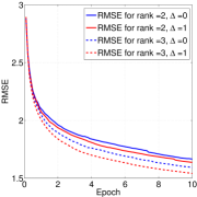
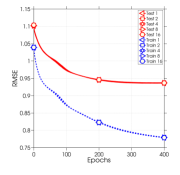
In particular, we complete a matrix of rank 2 or 3, possibly using width-2 interval uncertainty set and scale of 1 to 5 stars in the ratings. To illustrate the impact of the this change, we present the evolution of Root-Mean-Square Error (RMSE) in Figure 2 (left). Notice that an “epoch”, which is the unit on the horizontal axis, consists of element updates of matrix and element updates of matrix .
Let us remark that RMSE is sensitive to the choice of and the rank of the matrix we are looking for. If the underlying matrix has a higher rank than expected, can lead to smaller values of RMSE. We should also note that for some fixed and , RMSE can be better with for a few epochs, but then get worse when compared with . Hence, in practice, cross validation should be used to determine suitable value of parameter .
On the Yelp data set, we have performed 10-fold cross-validation on the training set, using varying rank. As we increased the rank from 1 to 2, 4, 8, 16, 32, and 50, the average error decreased from 1.7958 to 1.8284, 1.6464, 1.4590, 1.3395, 1.2702, and 1.2454, respectively. This seems to be comparable to the best results from the 2013 Recommender Systems Challenge444 https://www.kaggle.com/c/yelp-recsys-2013 , where a smaller dataset was used.
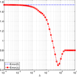
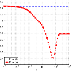
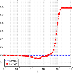
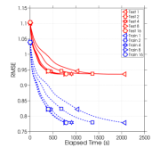
Further, one can illustrate the effects in a matrix-recovery experiment. We use random matrices of rank . We sample of entries of the matrix and store their indices in . We solve (4) with just the inequality constrains, i.e., , and , where is a matrix with all elements equals to . Let us denote by the solution of that optimization problem after serial iterations () and with . Figure 1 shows the dependence of error defined as follows where is the best rank approximation of obtain using SVD decomposition of the whole matrix. Figure 1 clearly suggest that, e.g., if of elements are observed then by allowing each entry of reconstructed matrix to lie in neighborhood of observed values, we can decrease the relative error of reconstruction from approximately to for . In this case, the value of was and .
 |
 |
 |
4.2 Image In-Painting
Further, we provide a comparison on the in-painting benchmark of [45]. Table 1 details the performance of SVT [6], SVP [16], SoftImpute [25], LMaFit [11], ADMiRA, [22], JS [15], OR1MP [45], and EOR1MP [45] on 10 well-known gray-scale images (Barbara, Cameraman, Clown, Couple, Crowd, Girl, Goldhill, Lenna, Man, Peppers) of pixels each. of pixels were removed uniformly at random, and the image was reconstructed using rank 50. The performance was measured in terms of PSNR, which is for mean squared error . Our approach with inequalities dominates all other approaches on 7 out of the 10 images. On the remaining 3 images, one would have to use the extrema of the observed elements, e.g., a subinterval of 12–246 for Barbara.
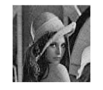
To illustrate the aggregate results further, we undertook the following experiment. We took a gray scale image (Lenna) and chose of the pixels randomly, indexed as . Then, we ran Algorithm 1 for serial iterations (). We obtained solutions and , where was obtained when we used only equality constrains () and was obtained when we used also inequality constrains (, , , and is a set of all elements of except those in ). Figure 3 shows for different the best rank approximation obtained by SVD () and solutions and . The benefit of obvious inequality constrains is nicely visible, e.g., at , where the relative error of reconstruction is more than twice smaller. Further, the image is more smooth, upon visual inspection.
| rank | |||
|---|---|---|---|
| 30 |  |
 |
 |
| 50 |  |
 |
 |
| 100 |  |
 |
 |
| Instance / Algo. | SVT | SVP | SoftImpute | LMaFit | ADMiRA | JS | OR1MP | EOR1MP | MACO |
|---|---|---|---|---|---|---|---|---|---|
| Barbara | 26.9635 | 25.2598 | 25.6073 | 25.9589 | 23.3528 | 23.5322 | 26.5314 | 26.4413 | 23.8015 |
| Cameraman | 25.6273 | 25.9444 | 26.7183 | 24.8956 | 26.7645 | 24.6238 | 27.8565 | 27.8283 | 28.9670 |
| Clown | 28.5644 | 19.0919 | 26.9788 | 27.2748 | 25.7019 | 25.2690 | 28.1963 | 28.2052 | 29.0057 |
| Couple | 23.1765 | 23.7974 | 26.1033 | 25.8252 | 25.6260 | 24.4100 | 27.0707 | 27.0310 | 27.1824 |
| Crowd | 26.9644 | 22.2959 | 25.4135 | 26.0662 | 24.0555 | 18.6562 | 26.0535 | 26.0510 | 26.1705 |
| Girl | 29.4688 | 27.5461 | 27.7180 | 27.4164 | 27.3640 | 26.1557 | 30.0878 | 30.0565 | 30.4110 |
| Goldhill | 28.3097 | 16.1256 | 27.1516 | 22.4485 | 26.5647 | 25.9706 | 28.5646 | 28.5101 | 28.6265 |
| Lenna | 28.1832 | 25.4586 | 26.7022 | 23.2003 | 26.2371 | 24.5056 | 28.0115 | 27.9643 | 28.3581 |
| Man | 27.0223 | 25.3246 | 25.7912 | 25.7417 | 24.5223 | 23.3060 | 26.5829 | 26.5049 | 26.5990 |
| Peppers | 25.7202 | 26.0223 | 26.8475 | 27.3663 | 25.8934 | 24.0979 | 28.0781 | 28.0723 | 28.8469 |
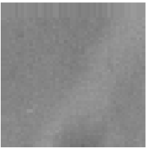
Further, we took a image and sampled randomly 50% of pixels. (The image is the top-left corner of the Lenna image.) Figure 4 shows the original image and the best rank 10 approximation . The solutions , , and were obtained by running Algorithm 1 for serial iterations (), where contains the observed pixels and and contains all other pixels. We have used and . The result again suggest that adding simple and obvious constrains leads to better low rank reconstruction and helps to keep reconstructed elements of matrix in expected bounds.
 |
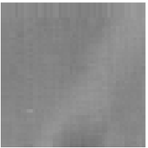 |
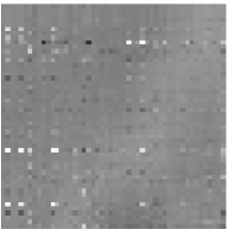 |
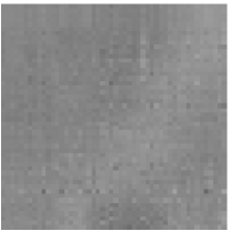 |
 |
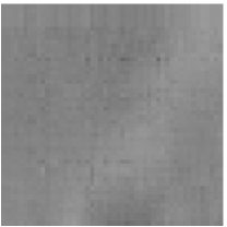 |
4.3 The Run-Time
Finally, in order to illustrate the run-time and efficiency of parallelization of Algorithm 1, Figure 2 (right) presents the evolution of RMSE over time on the well-known matrix of rank 20. There is an almost linear speed-up visible from 1 to 4 cores and marginally worse speed-up between 4 and 8 cores. Considering that most other algorithms proposed in the literature cannot cope with instances of this size, we cannot compare the performance directly to SVT [6], SVP [16], SoftImpute [25], LMaFit [11], ADMiRA, [22], JS [15], OR1MP [45], EOR1MP [45], and similar. We can, however, compare the run-time on the instances, detailed in Table 1.
5 Conclusions
We have studied the matrix completion problem under interval uncertainty and an efficient algorithm, which converges to stationary points of the NP-Hard, non-convex optimisation problem, without ever trying to approximate the spectrum of the matrix. In our computational experiments, we have shown that even the seemingly most trivial inequality constraints are useful in a number of applications. This opens numerous avenues for further research:
-
•
Forecasting with Side Information: A related application comes from the forecasting of seasonal data, e.g. sales. Let us assume that in process , one knows such that for the cumulative distribution function of the joint distribution of at times . One can then formulate the forecasting into the future as a matrix completion problem, where there the historical datum at time is at row , column specified by an equality or a pair of inequalities, and where inequalities represent side information. For example in sales forecasts, one often has bookings for many months in advance and knows that the sales for the respective months will not be less than the bookings taken.
-
•
Non-negative matrix factorization: The coordinate descent algorithm for the problem (4) is easy to extend, e.g., toward non-negative factorization. It is sufficient to modify lines 7 and 13 in Algorithm 1 as follows: , . One could consider extensions beyond box constraints on the individual elements as well.
-
•
Auto-tuning : If we have some a priori bound on the largest eigenvalue of the matrix to reconstruct, let us denote it , then we can modify lines 7 and 13 in Algorithm 1 as follows , .
We would be delighted to share our code with other researchers interested in these and related problems. Currently, the code is available from http://optml.github.io/ac-dc/. Should it become unavailable, for any reason, we encourage researchers to contact us.
References
- [1] Carlos M. Alaíz, Francesco Dinuzzo, and Suvrit Sra. Correlation matrix nearness and completion under observation uncertainty. IMA J. Numer. Anal., 35(1):325–340, 2013.
- [2] R.M. Bell and Y. Koren. Scalable collaborative filtering with jointly derived neighborhood interpolation weights. In ICDM, pages 43–52, Oct 2007.
- [3] Jian-Feng Cai, Emmanuel J Candès, and Zuowei Shen. A singular value thresholding algorithm for matrix completion. SIAM J. Optim., 20(4):1956–1982, 2010.
- [4] Emmanuel J Candès, Xiaodong Li, Yi Ma, and John Wright. Robust principal component analysis? J. Assoc. Comput. Mach., 58(3):11, 2011.
- [5] Emmanuel J Candès and Yaniv Plan. Matrix completion with noise. Proc. IEEE, 98(6):925–936, 2010.
- [6] Emmanuel J Candès and Benjamin Recht. Exact matrix completion via convex optimization. FoCM, 9(6):717–772, 2009.
- [7] Yudong Chen, Huan Xu, Constantine Caramanis, and Sujay Sanghavi. Robust matrix completion with corrupted columns. pages 873–880, 2011.
- [8] Yuxin Chen and Yuejie Chi. Spectral compressed sensing via structured matrix completion. In ICML, pages 414–422, 2013.
- [9] Alexander L Chistov and D Yu Grigor’ev. Complexity of quantifier elimination in the theory of algebraically closed fields. In MFCS, pages 17–31. Springer, 1984.
- [10] Maryam Fazel. Efficient Algorithms for Collaborative Filtering. PhD thesis, Stanford University, 2002.
- [11] Donald Goldfarb, Shiqian Ma, and Zaiwen Wen. Solving low-rank matrix completion problems efficiently. In Allerton, pages 1013–1020. IEEE, 2009.
- [12] J.P. Haldar and D. Hernando. Rank-constrained solutions to linear matrix equations using powerfactorization. IEEE Signal Proc. Let., 16(7):584–587, July 2009.
- [13] Nathan Halko, Per-Gunnar Martinsson, and Joel A Tropp. Finding structure with randomness: Probabilistic algorithms for constructing approximate matrix decompositions. SIAM Rev., 53(2):217–288, 2011.
- [14] Nicholas JA Harvey, David R Karger, and Sergey Yekhanin. The complexity of matrix completion. In SODA, pages 1103–1111, 2006.
- [15] Martin Jaggi and Marek Sulovský. A simple algorithm for nuclear norm regularized problems. In ICML, pages 471–478, 2010.
- [16] Prateek Jain, Raghu Meka, and Inderjit S Dhillon. Guaranteed rank minimization via singular value projection. In NIPS, pages 937–945, 2010.
- [17] Prateek Jain, Praneeth Netrapalli, and Sujay Sanghavi. Low-rank matrix completion using alternating minimization. In STOC, pages 665–674, 2013.
- [18] R. Kannan, M. Ishteva, and Haesun Park. Bounded matrix low rank approximation. In ICDM, pages 319–328, Dec 2012.
- [19] Raghunandan H Keshavan, Andrea Montanari, and Sewoong Oh. Matrix completion from a few entries. IEEE T. Inf. Theory, 56(6):2980–2998, 2010.
- [20] Raghunandan Hulikal Keshavan. Efficient Algorithms for Collaborative Filtering. PhD thesis, Stanford University, 2012.
- [21] Y. Koren, R. Bell, and C. Volinsky. Matrix factorization techniques for recommender systems. Computer, 42(8):30–37, Aug 2009.
- [22] Kiryung Lee and Y. Bresler. Admira: Atomic decomposition for minimum rank approximation. IEEE T. Inf. Theory, 56(9):4402–4416, Sept 2010.
- [23] Guoyin Li, Alfred Ka Chun Ma, and Ting Kei Pong. Robust least square semidefinite programming with applications. Comput. Optim. App., 58(2):347–379, 2014.
- [24] Jakub Mareček, Peter Richtárik, and Martin Takáč. Distributed block coordinate descent for minimizing partially separable functions. In Numerical Analysis and Optimization, pages 261–288, 2015. Springer Proceedings in Math. and Statistics, Vol. 134.
- [25] Rahul Mazumder, Trevor Hastie, and Robert Tibshirani. Spectral regularization algorithms for learning large incomplete matrices. J. Mach. Learn. Res., 11:2287–2322, 2010.
- [26] Bhaskar Mehta, Thomas Hofmann, and Wolfgang Nejdl. Robust collaborative filtering. In RecSys, pages 49–56, New York, NY, USA, 2007. ACM.
- [27] Andriy Mnih and Ruslan Salakhutdinov. Probabilistic matrix factorization. In NIPS, pages 1257–1264, 2007.
- [28] Balas Kausik Natarajan. Sparse approximate solutions to linear systems. SIAM J. Comput., 24(2):227–234, 1995.
- [29] Yurii Nesterov. Efficiency of coordinate descent methods on huge-scale optimization problems. SIAM J. Optim., 22(2):341–362, 2012.
- [30] Benjamin Recht, Christopher Ré, Stephen J. Wright, and Feng Niu. Hogwild: A lock-free approach to parallelizing stochastic gradient descent. In NIPS, pages 693–701, 2011.
- [31] Jasson D. M. Rennie and Nathan Srebro. Fast maximum margin matrix factorization for collaborative prediction. In ICML, ICML ’05, pages 713–719, New York, NY, USA, 2005. ACM.
- [32] Peter Richtárik and Martin Takáč. Iteration complexity of randomized block-coordinate descent methods for minimizing a composite function. Math. Program., 144(2):1–38, 2014.
- [33] Peter Richtárik and Martin Takáč. On optimal probabilities in stochastic coordinate descent methods. Optim. Lett., pages 1–11, 2015.
- [34] Peter Richtárik and Martin Takáč. Distributed coordinate descent method for learning with big data. J. Mach. Learn. Res., to appear, 2016.
- [35] Peter Richtárik and Martin Takáč. Parallel coordinate descent methods for big data optimization. Math. Program., 156(1):433–484, 2016.
- [36] Badrul Sarwar, George Karypis, Joseph Konstan, and John Riedl. Application of dimensionality reduction in recommender system-a case study. In WebKDD, 2000.
- [37] Shai Shalev-Shwartz, Alon Gonen, and Ohad Shamir. Large-scale convex minimization with a low-rank constraint. In ICML, pages 329–336, 2011.
- [38] Allen L. Soyster. Convex programming with set-inclusive constraints and applications to inexact linear programming. Oper. Res., 21(5):pp. 1154–1157, 1973.
- [39] Nathan Srebro. Learning with matrix factorizations. PhD thesis, MIT, 2004.
- [40] Nathan Srebro, Jason Rennie, and Tommi S Jaakkola. Maximum-margin matrix factorization. In NIPS, pages 1329–1336, 2004.
- [41] Jared Tanner and Ke Wei. Normalized iterative hard thresholding for matrix completion. SIAM J Sci. Comput., 35(5), 2013.
- [42] Rachael Tappenden, Peter Richtárik, and Burak Büke. Separable approximations and decomposition methods for the augmented lagrangian. Optim. Methods Softw., 30(3):463–668, 2015.
- [43] Rachael Tappenden, Martin Takáč, and Peter Richtárik. On the complexity of parallel coordinate descent. arXiv preprint arXiv:1503.03033, 2015.
- [44] Ryota Tomioka, Taiji Suzuki, Masashi Sugiyama, and Hisashi Kashima. A fast augmented lagrangian algorithm for learning low-rank matrices. In ICML, pages 1087–1094, 2010.
- [45] Zheng Wang, Ming-Jun Lai, Zhaosong Lu, Wei Fan, Hasan Davulcu, and Jieping Ye. Rank-one matrix pursuit for matrix completion. In ICML, pages 91–99, 2014.
- [46] John Wright, Arvind Ganesh, Shankar Rao, Yigang Peng, and Yi Ma. Robust principal component analysis: Exact recovery of corrupted low-rank matrices via convex optimization. In Y. Bengio, D. Schuurmans, J.D. Lafferty, C.K.I. Williams, and A. Culotta, editors, NIPS, pages 2080–2088. Curran Associates, Inc., 2009.
- [47] Jieping Ye. Generalized low rank approximations of matrices. Mach. Learn., 61(1-3):167–191, 2005.
Acknowledgements
The authors are grateful for the reviews, which have helped them to improve both the presentation and contents of the paper. In addition, the first author acknowledges funding from the European Union Horizon 2020 Programme (Horizon2020/2014-2020), under grant agreement number 688380. The second author would like to acknowledge support from the EPSRC Grant EP/K02325X/1, Accelerated Coordinate Descent Methods for Big Data Optimization.