Cell-type-specific neuroanatomy of brain-wide expression of autism-related genes
  Pascal Grange Department of mathematical sciences Xi’An Jiaotong-Liverpool University, Suzhou 215123, Jiangsu, China pascal.grange@xjtlu.edu.cn
Idan Menashe Department of Public Health, Faculty of Health Sciences Ben-Gurion University of the Negev, P.O.Box 653, Beer-Sheva 84105, Israel Michael Hawrylycz Allen Institute for Brain Science, Seattle, WA 98103, United States

Abstract

Two cliques of genes identified computationally for their high co-expression in the mouse brain according to the Allen Brain Atlas, and for their enrichment in genes related to autism spectrum disorder, have recently been shown to be highly co-expressed in the cerebellar cortex, compared to what could be expected by chance. Moreover, the expression of these cliques of genes is not homogeneous across the cerebellum, and it has been noted that their gene expression pattern seems to highlight the granular layer. However, this observation was only made by eye, and recent advances in computational neuroanatomy allow to rank cell types in the mouse brain (characterized by their transcriptome profiles) according to the similarity between their density profiles and the expression profiles of the cliques. We establish by Monte Carlo simulation that with probability at least 99%, the expression profiles of the two cliques are more similar to the density profile of granule cells than 99% of the expression of cliques containing the same number of genes (Purkinje cells also score above 99% in one of the cliques). Thresholding the expression profiles shows that the signal is more intense in the granular layer.

Keywords. Computational neuroanatomy, gene expression, cerebellum, cell types, ASD.

Acronyms. ASD: autism spectrum disorder; ABA: Allen Brain Atlas; ISH: in situ hybridization; ARA: Allen Reference Atlas; CDF: cumulative distribution function.

1 Introduction

The neuroanatomical structures underlying autism spectrum disorder (ASD) traits are the subject of intense research efforts, as ASD is one of the most prevalent and highly heritable neurodevelopmental disorders in humans [1, 2, 3, 4]. A good source of data for such studies is the Allen Brain Atlas (ABA) of the adult mouse [5, 6, 7, 8, 9, 10, 11, 12, 13, 14], which consists of thousands of brain-wide in situ hybridization (ISH) gene-expression profiles, co-registered to the Allen Reference Atlas (ARA) [15]. Recently, we used the ABA to examine the spatial co-expression characteristics of genes associated with autism susceptibility [16]. We identified two networks of co-expressed genes that are enriched with autism genes and which are significantly overexpressed in the cerebellar cortex.

These results added to the mounting evidence of the involvement of the cerebellum in autism [17, 18]. However, the rich internal structure of cerebellum requires a further investigation of the specific cerebellar regions or cell types associated with ASD.

In our paper [16] we indicated that the two cliques of co-expressed autism genes appear to be overexpressed in the granular layer of the cerebellum. However, this observation was based on visual comparison of the expression patterns of the genes in these two cliques to sections of the estimated density patterns of cell types, which at the time were available as preprint from [19]. This approach by mere visual inspection is far from satisfactory since it does not make use of the full computational power of the ABA [20, 21, 22, 23]. Moreover, post-mortem studies of brains of autistic patients [24] have shown alterations in the Purkinje layer of the cerebellum, rather than in the granule cells.

In the present study we re-examine the two cliques discovered in [16] using recent developments of computational neuroanatomy relating cell-type-specificity of gene expression to neuroanatomy based on the ABA. For example, in [25, 19, 26], the region-specificity of 64 cell types (collated from [27, 28, 29, 30, 31, 32, 33, 34, 35]) was estimated using a linear mathematical model, which amounts to decomposing the gene expression in the ABA over a set of measured cell-type-specific transcriptomes (see also [36, 37] for cell-type-specific analyses of the ABA, and [38] for a similar mathematical approach in the context of blood cells). We extend the Monte Carlo methods (developed in [16] to estimate the probability of co-expression among a set of genes) to the comparison between the expression of a set of genes and the spatial density profile of a cell type. This allows to estimate not only the probability of the similarity between a gene clique and the granular layer, but also the probabilities of similarity to the spatial distributions of all cell types considered in [25].

2 Methods

Cliques of genes. We re-examine the brain-wide expression profiles of the two cliques $\mathcal{C}_{1}$ and $\mathcal{C}_{2}$ of genes identified in [16] based on their exceptional co-expression profiles, which consist of 33 and 6 genes respectively:

$$\begin{array}[]{ll}\mathcal{C}_{1}&=\{Astn2,Dpp6,Galnt13,Ptchd1,Trim3,Slc12a3,\\ &Pltp,Mpp3,Darc,B230317C12Rik,Pla2g7,Syt2,\\ &Edg1,Cnr1,0610007P14Rik,Socs5,Atp1a1,Chgb,\\ &Car4,Pcbp4,Syne1,Camk2d,Slc6a1,C230009H10Rik,\\ &LOC434631,Prpf38b,D530033C11Rik,Coro2b,Tmem109,Daam2,\\ &Gpr37l1,BC060632,Grm4\},\end{array}$$ (1)

$$\begin{array}[]{ll}\mathcal{C}_{2}=\{Rims3,Astn2,B230308C24Rik\ast,LOC434631,4933417O08Rik,Car10\}.\end{array}$$ (2)

They both contain genes from the AutRefDB database ([39, 40]) of ASD-related genes(Ptchd1, Galnt13, Dpp6 and Astn2 for the first clique, Astn2 and Rims3 for the second).

Gene expression energies from the Allen Brain Atlas. The adult mouse brain is partitioned into $V=49,742$ cubic voxels of side 200 microns, to which ISH data are registered [15, 8] for thousands of genes. For computational purposes, these gene-expression data can be arranged into a voxel-by-gene matrix. For a cubic voxel labeled $v$, the expression energy of the gene $g$ is a weighted sum of the greyscale-value intensities evaluated at the pixels intersecting the voxel:

$$E(v,g)={\mathrm{expression\;energy\;of\;gene\;labeled\;}}g\;{\mathrm{in\;voxel\;labeled\;}}v,$$ (3)

The present analysis is restricted to the coronal atlas, as in [21, 23, 16], for which the entire mouse brain was processed in the ABA pipeline (whereas only the left hemisphere was processed for the sagittal atlas)

Cell-type-specific microarray data and estimated cell-type-specific density profiles . The cell-type-specific microarray reads collated in [35] from the studies [27, 28, 29, 30, 31, 32, 33, 34] (for $T=64$ different cell-type-specific samples) are arranged in a type-by-gene matrix denoted by $C$, such that

$$C(t,g)={\mathrm{expression\;of\;gene\;labeled\;}}g\;{\mathrm{in\;cell\;type\;labeled\;}}t,$$ (4)

and the columns are arranged in the same order as in the matrix $E$ of expression energies defined in Eq. 3. In [25], we proposed a simple linear model for a voxel-based gene-expression atlas in terms of the transcriptome profiles of individual cell types and their spatial densities:

$$E(v,g)=\sum_{t}\rho_{t}(v)C(t,g)+{\mathrm{Residual}}(v,g),$$ (5)

where the index $t$ denotes the $t$-th cell type, with density profile $\rho_{t}(v)$ at voxel labeled $v$. The values of the cell-type-specific density profiles were computed in [25] by minimizing the value of the residual term over all the (positive) density profiles, which amounts to solving a quadratic optimization problem at each voxel.

Measure of similarity between gene-expression patterns and cell-type-specific density patterns. The quantitative study of spatial co-expression of genes conducted in [16] combines the columns of the matrix of gene-expression energies (Eq. 3) by computing the cosine similarities of all pairs of genes in the cliques $\mathcal{C}_{1}$ and $\mathcal{C}_{2}$. These cosine similarities are then compared to those obtained from random sets of genes containing the same numbers of elements as $\mathcal{C}_{1}$ and $\mathcal{C}_{2}$ respectively. This technique can be adapted to compare brain-wide gene-expression profiles to the spatial density of cell types, simply by considering cosine similarities between gene-expression profiles and cell-type-specific density profiles.
Given a set $\mathcal{G}$ of genes from the coronal ABA (selected either computationally based on their co-expression properties, or based on curation of the biomedical literature, which in the present case means $\mathcal{G}=\mathcal{C}_{1}$ or $\mathcal{G}=\mathcal{C}_{2}$), we can compute the sum of their expression profiles:

$$E^{\mathcal{G}}(v)=\sum_{i=1}^{|\mathcal{G}|}E(v,g_{i}),$$ (6)

where $g_{i}$ is the column index in the matrix of expression energies (Eq. 3) corresponding to the $i$-th gene in the set $\mathcal{G}$. The quantity $E^{\mathcal{G}}$ is an element of $\mathbf{R}_{+}^{V}$, just as the estimated brain-wide density profile of a cell type. We can therefore estimate the similarity between $E^{\mathcal{G}}$ and the density of cell type labeled $t$ by computing the cosine similarity

$$\psi(\mathcal{G},t)=\frac{\sum_{v=1}^{V}E^{\mathcal{G}}(v)\rho_{t}(v)}{\sqrt{\sum_{u=1}^{V}E^{\mathcal{G}}(u)^{2}}\sqrt{\sum_{w=1}^{V}\rho_{t}(w)^{2}}},$$ (7)

which is between 0 and 1 by construction.

Statistical significance of the similarity between expression patterns and density patterns of cell types. Furthermore, for a fixed cell type, we can estimate how exceptional the similarity $\psi(\mathcal{G},t)$ is, compared to what would be expected from random sets of $|\mathcal{G}|$ genes drawn from the coronal ABA. This is a finite problem, but it becomes hugely complex in a regime where $|\mathcal{G}|$ is relatively large but still small compared to the size of the entire atlas (which is the case for both cliques in the present study). We can take a Monte Carlo approach, draw $R$ random sets of $|\mathcal{G}|$ genes and simulate the cumulative distribution function (CDF) of the cosine similarity between a random set of $|\mathcal{G}|$ genes and the density profile of cell-type labeled $t$ (this function depends only on the cell type and on the number of genes $|\mathcal{G}|$, we can denote it by ${\sc{\mathrm{CDF}}}_{t,|\mathcal{G}|}$). If we denote by $\mathcal{G}_{1}$, $\mathcal{G}_{2}$,… $\mathcal{G}_{R}$ random subsets of $[1..G]$ (drawn without repetition), we obtain an estimate an estimate of the CDF that reads as:

$${\sc{\mathrm{CDF}}}_{t,|\mathcal{G}|,R}(x):=\frac{1}{R}\sum_{r=1}^{R}\mathbf{1}\left(\psi(\mathcal{G}_{r},t)\geq x\right)\;\longrightarrow_{R\infty}{\sc{\mathrm{CDF}}_{t,|\mathcal{G}|}(x)}.$$ (8)

Moreover, the probability of obtaining a similarity to $\rho_{t}$ larger than a threshold $\psi(\mathcal{G},t)$ is estimated by:

$$\mathcal{P}_{R}(\mathcal{G},t):={\sc{\mathrm{CDF}}}_{t,|\mathcal{G}|,R}(\psi(\mathcal{G},t))=\frac{1}{R}\sum_{r=1}^{R}\mathbf{1}\left(\psi(\mathcal{G}_{r},t)\geq\psi(\mathcal{G},t)\right).$$ (9)

The precision of our estimates depends on the value of $R$. We can use Hoeffding’s inequality to compute a lower bound on the number $R$ of random draws required to estimate the probability of being within a known error from the true CDF. As we are estimating the probability of having larger cosine similarity than expected by chance by summing $R$ Bernoulli variables (Eq. 9), Hoeffding’s inequality (see [41] for instance) states that for any $\tau$, the probability of missing the true value of the probability $\mathcal{P}(\mathcal{G},t)$ by $\tau$ is bounded in terms of $\tau$ and the number of random draws $R$ as follows:

$$P(|\mathcal{P}_{R}(\mathcal{G},t)-\mathcal{P}(\mathcal{G},t)|\geq\tau)\leq\exp(-2R\tau^{2}).$$ (10)

For instance, taking $\tau=0.01$ and $R=26,500$ leads to a value of $0.01$ for the bound on the r.h.s. of the inequality 10, so it is enough to draw this number of random sets of genes to obtain an estimator within 1 percent of the true probabilities, with probability at least 99 percent.

Having conducted the simulation of the distribution of cosine similarities for a choice of $R$ based on Hoeffding’s inequality, we can rank cell types for a fixed clique $\mathcal{G}$ by decreasing values of statistical significance:

$${\mathcal{P}}_{R}(\mathcal{G},t_{\mathcal{G}}(1))\geq{\mathcal{P}}(\mathcal{G},t_{\mathcal{G}}(2))\geq...\geq{\mathcal{P}}_{R}(\mathcal{G},t_{\mathcal{G}}(T)).$$ (11)

Similarity between thresholded gene-expression energies and cell-type-specific densities. Given that the expression profiles of the cliques is much less sparse than any of the densities of cell types estimated in [25], the genes in the cliques must be expressed in several different cell types, but there are large differences in expression between cortical voxels and cerebellar voxels for instance, and also within the cerebellar cortex (see Fig. 1a,b). We propose to threshold brain-wide expression profile of each clique, and to recompute the cosine similarities with density profiles, in order to discover which neuroanatomical cell-type-specific patterns are highlighted with more intensity. If the profile of a given cell type is highlighted by a given clique, when the threshold grows from zero to low values of the threshold, the cosine similarity is expected to grow, since many voxels with low values of expression energy, that penalize the cosine similarity to the cell type, are put to zero by the threshold. Let us denote by $\tau$ the value of the threshold. We can compute the thresholded expression energies of the cliques and cosine similarities as follows:

$$E^{\mathcal{G}}_{\tau}(v)=E^{\mathcal{G}}(v)\mathbf{1}\left(E^{\mathcal{G}}(v)\geq\tau\right),$$ (12)

$$\psi_{\tau}(\mathcal{G},t)=\frac{\sum_{v=1}^{V}E^{\mathcal{G}}_{\tau}(v)\rho_{t}(v)}{\sqrt{\sum_{u=1}^{V}E_{\tau}^{\mathcal{G}}(u)^{2}}\sqrt{\sum_{w=1}^{V}\rho_{t}(w)^{2}}},$$ (13)

At very large values of the threshold, expression energies are going to be put to zero everywhere, and the cosine similarities decrease to zero. So the cosine similarity between the expression of the two gene cliques and the cell types they highlight are expected to exhibit peaks when plotted as a function of the threshold. The higher the peak, and the higher the corresponding value of the threshold, the more intensely the cell type is highlighted.

3 Results

We computed the cosine similarities between the expression profiles of the two cliques ${\mathcal{C}}_{1}$ and ${\mathcal{C}}_{2}$ and the density profiles of the $T=64$ cell types estimated in [25], using Eq. 7. For each cell type, we computed the probabilities $\mathcal{P}_{R}({\mathcal{C}}_{1},t)$ and $\mathcal{P}_{R}({\mathcal{C}}_{2},t)$ for $R=27,000$. Tables 1b show the cell types for which the cosine similarity is larger than 10%, ordered by decreasing values of statistical significance. For both cliques, granule cells (labeled $t=20$) and Purkinje cells (labeled $t=1$), have the highest value of $P_{R}$ (more than 99% for both cliques in the case of granule cells). For each of the two cliques, one more cell type has a value of $P_{R}$ larger than 80% (mature oligodendrocytes, labeled $t=21$, in the case of ${\mathcal{C}}_{1}$, pyramidal neurons, labeled $t=46$, in the case of ${\mathcal{C}}_{2}$). The statistical significance (i.e. the value of ${\mathcal{P}}_{R}$) drops sharply after the third rank for both cliques. Our computational analysis therefore returns a list of four cell types to which at least one of the two cliques in this study are more similar than at least 80% of the sets of genes of the same cardinality as the cliques.

Figure 1 shows heat maps of the expression profiles of the two cliques and of the density profiles of these four cell types. The expression profiles of both cliques highlight the cerebellum, but they are non-zero in many more voxels than any of the densities of cell types illustrated in Fig. 1c1–c4. These densities are highly concentrated in the cerebellum (indeed the corresponding cell-type-specific samples were extracted from the cerebellum, see [30] for Purkinje cells, see[33] for granule cells labeled and mature oligodendrocytes), with the exception of the pyramidal neurons (labeled $t=46$) which are highly localized in the cerebral cortex (the corresponding cell-type-specific samples were extracted from the layer 5 of the cerebral cortex, see [27]).

Table 1: Tables of cell types ordered by decreasing values of statistical significance (see Eq. 11), measured by the probability $\mathcal{P}_{R}(\mathcal{G},t)$, for $R=27,000$. Only cell types for which the cosine similarity is larger than 10% are shown. (a) For clique 1, $\mathcal{G}=\mathcal{C}_{1}$. (b) For clique 2 $\mathcal{G}=\mathcal{C}_{2}$. The top three cell types for each of the cliques have a value of $\mathcal{P}_{R}(\mathcal{G},t)$ higher than $80\%$, and together they consist of four distinct cell types, whose density profiles are illustrated in Fig. 1c(1–4).

Cell type	Rank by significance, $t_{\mathcal{C}_{1}}^{-1}(t)$	Index $t$	$\mathcal{P}_{R}(\mathcal{C}_{1},t)$, (%)	$\psi(\mathcal{C}_{1},t)$, (%)
Purkinje Cells	1	1	100	45.9
Granule Cells	2	20	100	42.4
Mature Oligodendrocytes	3	21	99.5	12.7
GABAergic Interneurons, PV+	4	64	38.4	35.3
GABAergic Interneurons, PV+	5	59	37.6	11.3
GABAergic Interneurons, SST+	6	57	36.1	22.1
GABAergic Interneurons, SST+	7	56	34.8	16

(a)

Cell type	Rank by significance, $t_{\mathcal{C}_{2}}^{-1}(t)$	Index $t$	$\mathcal{P}_{R}(\mathcal{C}_{2},t)$, (%)	$\psi(\mathcal{C}_{2},t)$, (%)
Granule Cells	1	20	99.4	46.1
Purkinje Cells	2	1	97.8	42.5
Pyramidal Neurons	3	46	81.7	47.1
Mature Oligodendrocytes	4	21	72.6	10.2
GABAergic Interneurons, PV+	5	59	67.2	12.2

(b)

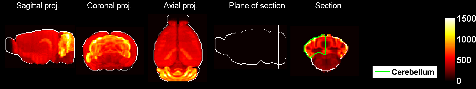
(a)

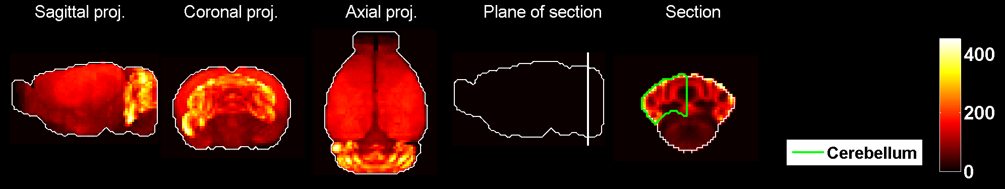
(b)

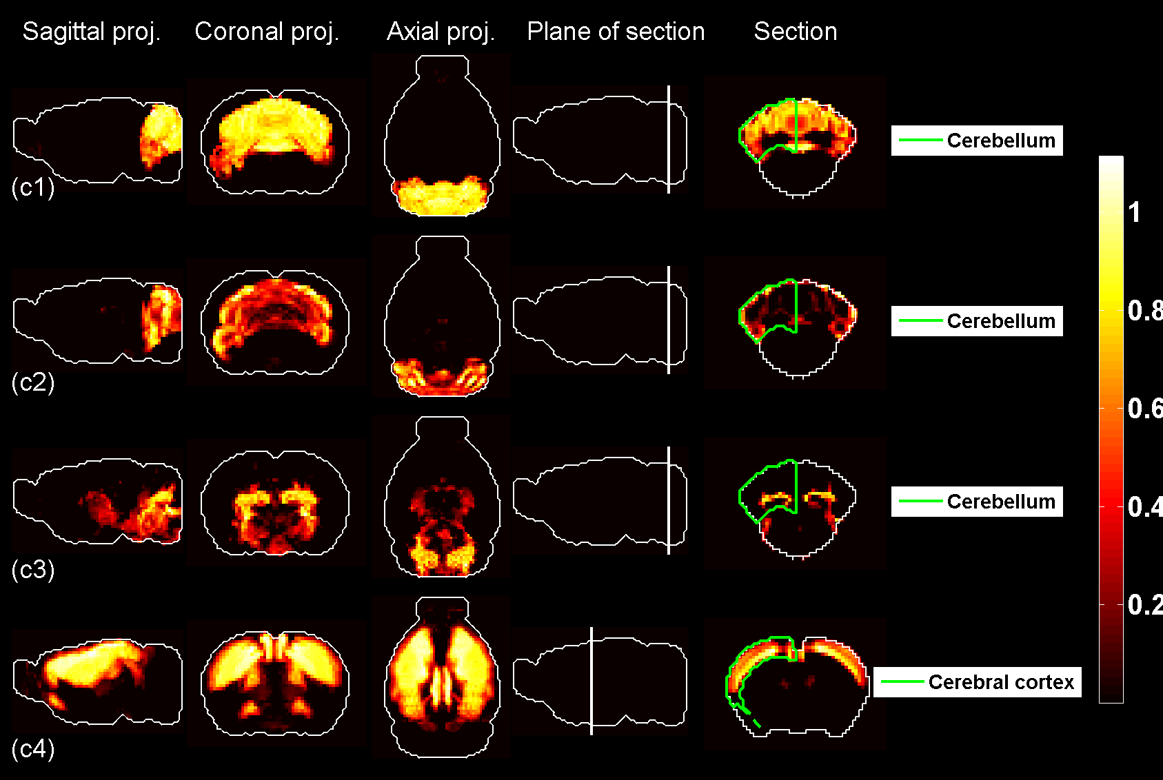
(c)

Figure 1: Heat maps of gene-expression of gene cliques, and of density profiles of cell types. (a) Heat map of the sum of expression energies of the 33 genes in the clique ${\mathcal{C}}_{1}$. (b) Heat map of the sum of expression energies of the 33 genes in the clique ${\mathcal{C}}_{2}$. (c) Heat maps of brain-wide densities (denoted by $\rho_{t}$ for cell type labeled $t$) of cell types estimated based on the model of Eq. 5, for Purkinje cells (c1, labeled $t=1$), granule cells (c2, labeled $t=20$), cerebellar mature oligodendrocytes (c3, labeled $t=21$), and cortical pyramidal neurons extracted from layer 5 (c4, labeled $t=46$). These four cell types are the ones that are ranked the most highly by statistical significance of similarity to either of the cliques $\mathcal{C}_{1}$ and $\mathcal{C}_{2}$.

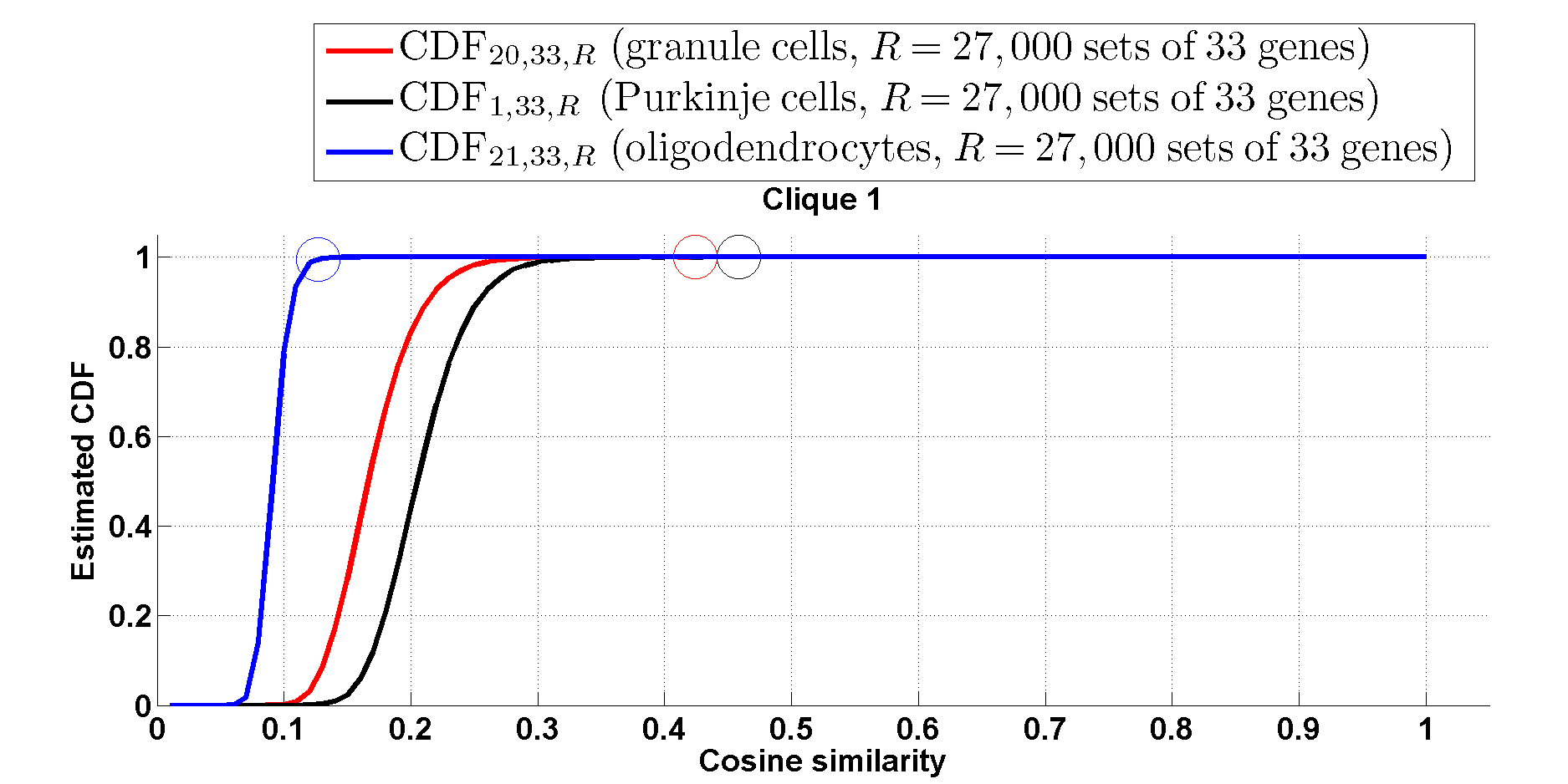
(a)

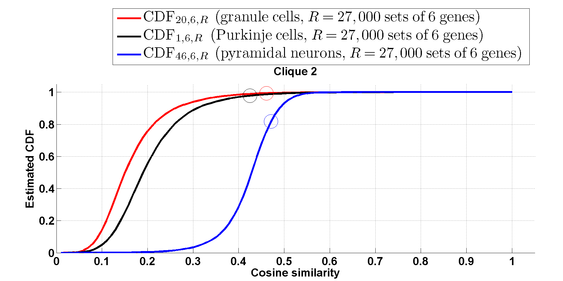
(b)

Figure 2: Simulated cumulative distribution functions (CDFs) of cosine similarities between gene-expression of cliques and the estimated density profile of the cell types whose density most resembles one or two of the two cliques (granule cells and Purkinje cells for both cliques, along with mature oligodendrocytes for $\mathcal{C}_{1}$ and pyramidal neurons for $\mathcal{C}_{2}$ . The values of the CDFs at the cosine similarities $\psi(\mathcal{G},t)$, for clique labeled $\mathcal{G}$ and cell type labeled $t$, are plotted as colored circles. The values of the probability $\mathcal{P}_{R}(\mathcal{G},t)$ are found in the third column of Table 1a,b (see Eq. 9). The plots show that granule cells and Purkinje cells both sit extremely comfortably at the top of the distribution of cosine similarities to the expresion of the clique.

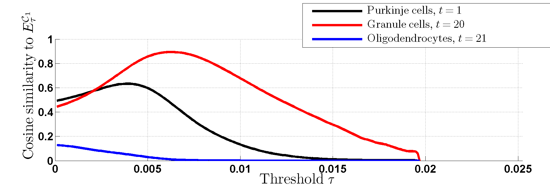
(a)

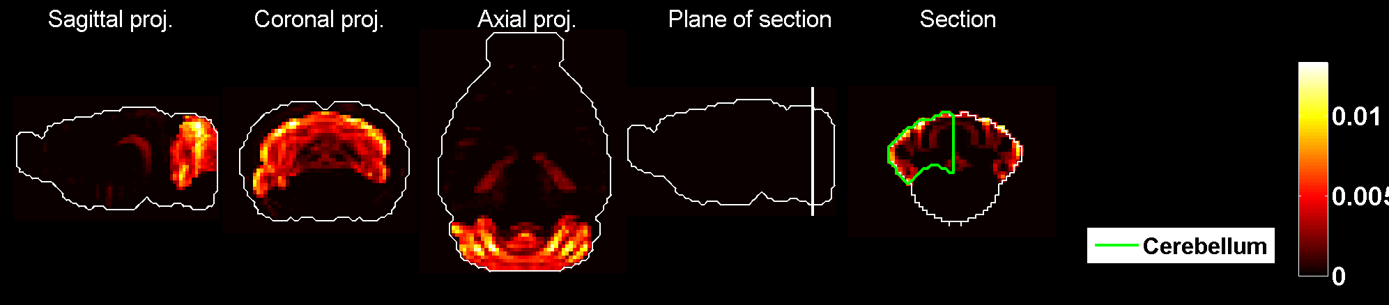
(b)

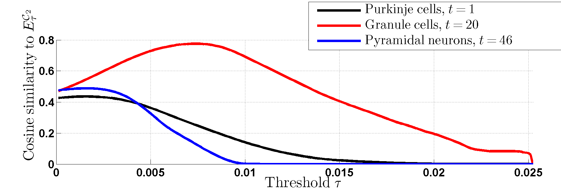
(c)

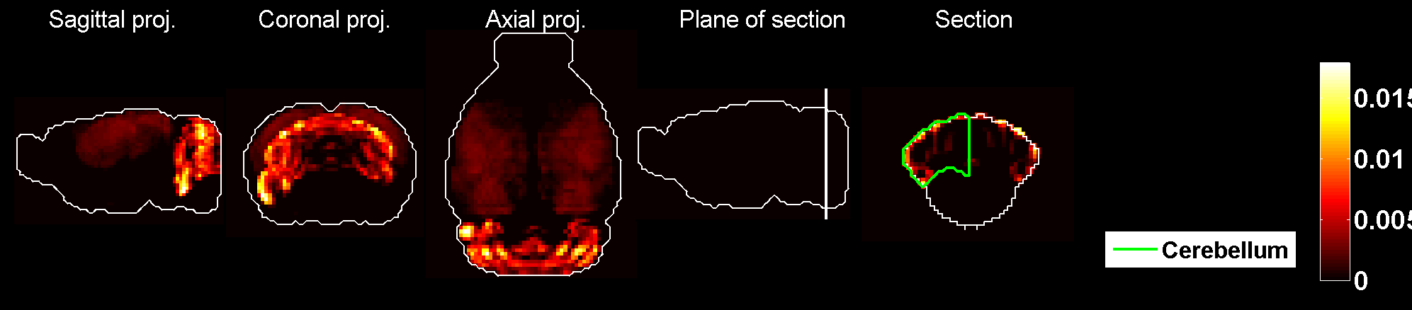
(d)

Figure 3: Cosine similarities of thresolded gene expression energies of cliques, as a function of the threshold (the expression profiles of the cliques are $L^{2}$-normalized so that threshold parameter $\tau$ interpolates between the minimum and maximal value of each of them, and stays in the same range). (a) Plot of $\psi_{\tau}(\mathcal{C}_{1},t)$ as a function of $\tau$ for the top three cell types in Table 1a. (c) Plot of $\psi_{\tau}(\mathcal{C}_{1},t)$ as a function of $\tau$ for the top three cell types in Table 1b. (b) Heat map of the expression energy of clique $\mathcal{C}_{1}$ at the value of the threshold $\tau$ for which $\psi_{\tau}(\mathcal{C}_{1},20)$ is maximum. (d) Heat map of the expression energy of clique $\mathcal{C}_{2}$ at the value of the threshold $\tau$ for which $\psi_{\tau}(\mathcal{C}_{2},20)$ is maximum.

The cell-type-specific sample of granule cells, (labeled $t=20$) is the only cell type that has a score higher than $99\%$ in both cliques. Figure 2 shows plots of the simulated CDFs of the cosine similarities between the top three cell types by significance and sets of genes of the same size as ${\mathcal{C}}_{1}$ (Fig. 2a) and ${\mathcal{C}}_{2}$ (Fig. 2b). One can observe that both granule cells and Purkinje cells sit more comfortably at the top of the distribution than the cell type ranked third by statistical significance, especially for clique $\mathcal{C}_{2}$.

We therefore need to vary the contrast in the presentation of the expression patterns, in order to decide in which sense, if any, the density profiles of granule cells and Purkinje cells are highlighted differently by the cliques $\mathcal{C}_{1}$ and $\mathcal{C}_{2}$. We computed the cosine similarities between cell types and thresholded expression profiles of the two cliques, as defined by Eq. 13. The values are plotted as a function of the threshold in Fig. 3a,c. Granule cells present a peak for both cliques (Purkinje cells do only for the clique $\mathcal{C}_{1}$, but at a lower value of the threshold and the top of the peak is lower, even though Purkinje cells start from a larger similarity to the clique $\mathcal{C}_{1}$ than granule cells before any threshold is applied). On the other hand, the thresholding procedure lowers the similarity between both cliques and the third cell type returned by the statistical analysis (oligodendrocytes for $\mathcal{C}_{1}$ and pyramidal neurons for $\mathcal{C}_{2}$. Moreover, Figure 3b,d) shows heat maps of the expression profiles of both cliques, at the values corresponding to the peak of cosine similarity to granule cells. Indeed the coronal sections through the cerebellum exhibit the characteristic layered, hollow profile of the density of granule cells observed in Fig. 1c2, which confirms that the granular layer is highlighted with more intensity by the cliques than the Purkinje layer. Maximal-intensity projections of the thresholded expression profiles exhibit residual expression in the cortex for clique $\mathcal{C}_{2}$, and to a lesser extent in the hippocampus for clique $\mathcal{C}_{1}$ (but it should be noted that genes are more highly expressed in the hippocampus than in any other region of the brain on average in the coronal ABA).

We therefore conclude that the gene expression profiles of the two cliques of genes in this study highlight the cerebellum with more intensity in the granular layer than in the Purkinje layer, but these two neuroanatomical structures are by far the most exceptionally similar to the expression profiles of the cliques.

4 Discussion

Our computational analysis shows that among the cell types analyzed in [25], the similarity of the expression of both cliques to granule cells and Purkinje cells is larger than the similarity of more than 97% of the cliques of the same size, and these two cell types are the only cell types in the panel to have this property. The statistical significance of the similarity to the spatial density of granule cells is larger than the one of Purkinje cells for the clique ${\mathcal{C}}_{2}$, but still Purkinje cells stand out together with granule cells (which makes sense with the involvement of Purkinje cells in autism discovered in post-mortem studies [24]). This completes our previous conclusion, reached in [16] by visual inspection of the Purkinje and granular layers of the cerebellar cortex. Granule cells (and not Purkinje cells) may be present in some superficial voxels in which both cliques are highly expressed (see the coronal sections in 1), but as brain-wide neuroanatomical patterns, granule cells and Purkinje cells are both exceptionally similar to the expression profiles of the two cliques in this study.

The values of the cosine similarities are not ranked in the same order as the statistical significances, because their values are not decreasing in the fourth columns of Tables 1a,b. This is related to the fact that the cosine similarity is biased in favor of cell types with a large support (and for example pyramidal neurons, $t=46$, have a larger support, at 8980 voxels, than granule cells, at 3351 voxels). So, if a clique of genes has a large support (which is the case of both cliques in this study, which have non-zero expression at more than $49,000$ voxels), it can have a larger cosine similarity to pyramidal neurons than to granule cells, but its similarity to granule cells may be more statistically significant. This is the case for clique $\mathcal{C}_{2}$, and the fact is illustrated in more detail on Fig. 2b, where it is clear that the similarity between pyramidal neurons (labeled $t=46$) and clique $\mathcal{C}_{2}$, albeit larger than the value for granule cells and Purkinje cells, sits lower in the distribution of the similarities. Our probabilistic approach is therefore a useful complement to the computation of cosine similarities.

Our analysis shows that the gene-based approach of the ABA and the cell-based approach of the transcriptional classification of cell types in the brain can be combined in order to quantify the similarity between expression patterns of condition-related genes. Our results are limited by the paucity of the cell-type-specific data, since the number of transcriptionally disctinct neuronal cell types is presumably much higher than $64$. However, the classification of cell types is a hierarchical problem, and it is plausible that granule cells and Purkinje cells branch early from each other (and from cortical pyramidal neurons and oligodendrocytes) in the classification, which makes the available data set reasonably effective as a first draft in the context of this study. The computational methods we devised can be easily reapplied when more cell-type-specific microarray data become available. Moreover, alternative measures of similarity can easily be substituted to the cosine similarity, without modifying the analysis of statistical significance and contrast, or the number of random draws dictated by Hoeffding’s inequality.

The spatial resolution of the voxelized ISH data of the mouse ABA (200 microns) complicates the separation between granule cells and Purkinje cells, which we attempted here by our thresholding procedure, due to the extreme difference in size between the two cell types. Granule cells and Purkinje cells may be present in the same voxel, and registration errors are therefore much larger in scale of a granule cell than in scale of a Purkinje cell. An interesting analysis for such analysis can be found in [37, 42], where image series rather than voxelized data are used.

The translation of results from the mouse model to humans is technically challenging, even though the ABA of the human brain has been released [43], because the human atlas cannot be voxelized, due to the size and paucity of the specimens. A first step in this direction of research involves the study of variability of gene expression between the mouse and human atlas in well-charted regions of the brain.

References

- [1] Levy, S. E. (2009). Schultz RT. Autism. Lancet, 374, 1627–1638.
- [2] Lord, C. (2011). Epidemiology: How common is autism?. Nature, 474(7350), 166–168.
- [3] Newschaffer CJ, Croen LA, Daniels J, Giarelli E, Grether JK, et al. (2007) The epidemiology of autism spectrum disorders. Annu Rev Public Health 28: 235–258.
- [4] Amaral DG, Schumann CM, Nordahl CW (2008) Neuroanatomy of autism. Trends Neurosci 31: 137–145.
- [5] Ng, L. et al. (2009), An anatomic gene expression atlas of the adult mouse brain, Nature Neuroscience 12, 356–362.
- [6] Jones AR, Overly CC, Sunkin SM (2009) The Allen Brain Atlas: 5 years and beyond. Nature Reviews (Neuroscience), Volume 10 (November 2009), 1.
- [7] Hawrylycz M, et al. (2011) Multi-scale correlation structure of gene expression in the brain. Neural Networks 24 (2011) 933–942.
- [8] Lein ES, et al. (2007) Genome-wide atlas of gene expression in the adult mouse brain, Nature 445, 168–176.
- [9] Ng L, Hawrylycz M, Haynor D (2005) Automated high-throughput registration for localizing 3D mouse brain gene expression using ITK. Insight-Journal (2005).
- [10] Sunkin SM, Hohmann JG (2007), Insights from spatially mapped gene expression in the mouse brain. Human Molecular Genetics, Vol. 16, Review Issue 2.
- [11] Hawrylycz M, et al. (2011), Digital Atlasing and Standardization in the Mouse Brain. PLoS Computational Biology 7 (2) (2011).
- [12] Ng L, et al. (2007) NeuroBlast: a 3D spatial homology search tool for gene expression. BMC Neuroscience, 8(Suppl 2):P11.
- [13] Ng L, et al. (2007) Neuroinformatics for genome-wide 3D gene expression mapping in the mouse brain. IEEE/ACM Trans. Comput. Biol. Bioinform., Jul-Sep 4(3) 382–93.
- [14] Lee CK, et al. (2008) Quantitative methods for genome-scale analysis of in situ hybridization and correlation with microarray data. Genome Biol. (2008); 9(1): R23.
- [15] Dong HW (2007), The Allen reference atlas: a digital brain atlas of the C57BL/6J male mouse, Wiley.
- [16] Menashe, I., Grange, P., Larsen, E. C., Banerjee-Basu, S., Mitra, P. P. (2013). Co-expression profiling of autism genes in the mouse brain. PLoS computational biology, 9(7), e1003128.
- [17] Reith, R. M., McKenna, J., Wu, H., Hashmi, S. S., Cho, S. H., Dash, P. K., Gambello, M. J. (2013). Loss of Tsc2 in Purkinje cells is associated with autistic-like behavior in a mouse model of tuberous sclerosis complex. Neurobiology of disease, 51, 93-103.
- [18] Lotta, L. T., Conrad, K., Cory-Slechta, D., Schor, N. F. (2014). Cerebellar Purkinje cell p75 neurotrophin receptor and autistic behavior. Translational psychiatry, 4(7), e416
- [19] Grange, P., Hawrylycz, M., Mitra, P. P. (2013). Cell-type-specific microarray data and the Allen atlas: quantitative analysis of brain-wide patterns of correlation and density. arXiv preprint arXiv:1303.0013.
- [20] Bohland JW et al. (2010) Clustering of spatial gene expression patterns in the mouse brain and comparison with classical neuroanatomy, Methods, 50(2), 105–112.
- [21] Grange P, Hawrylycz M, Mitra PP (2013), Computational neuroanatomy and co-expression of genes in the adult mouse brain, analysis tools for the Allen Brain Atlas. Quantitative Biology, 1(1): 91–100. (DOI) 10.1007/s40484-013-0011-5.
- [22] Grange P, Mitra PP (2012) Computational neuroanatomy and gene expression: optimal sets of marker genes for brain regions. IEEE, in CISS 2012, 46th annual conference on Information Science and Systems (Princeton).
- [23] Grange, P., Bohland, J. W., Hawrylycz, M., Mitra, P. P. (2012). Brain Gene Expression Analysis: a MATLAB toolbox for the analysis of brain-wide gene-expression data. arXiv preprint arXiv:1211.6177.
- [24] Skefos, J., Cummings, C., Enzer, K., Holiday, J., Weed, K., Levy, E., Bauman, M. (2014). Regional Alterations in Purkinje Cell Density in Patients with Autism. PloS one, 9(2), e81255.
- [25] Grange P, Bohland JW, Okaty BW, Sugino K, Bokil H, Nelson SB, Ng L, Hawrylycz M, Mitra PP, Cell-type–based model explaining coexpression patterns of genes in the brain, PNAS 2014 111 (14) 5397–5402.
- [26] Grange P, Bohland JW, Okaty BW, Sugino K, Bokil H, Nelson SB, Ng L, Hawrylycz M, Mitra PP (2014). Cell-type-specific transcriptomes and the Allen Atlas (II): discussion of the linear model of brain-wide densities of cell types. arXiv preprint arXiv:1402.2820.
- [27] Sugino K et al. (2005), Molecular taxonomy of major neuronal classes in the adult mouse forebrain. Nature Neuroscience 9, 99–107.
- [28] Chung CY et al. (2005), Cell-type-specific gene expression of midbrain dopaminergic neurons reveals molecules involved in their vulnerability and protection. Hum. Mol. Genet. 14: 1709–1725.
- [29] Arlotta P, et al. (2005), Neuronal subtype-specific genes that control corticospinal motor neuron development in vivo. Neuron 45: 207–221.
- [30] Rossner MJ, et al. (2006), Global transcriptome analysis of genetically identified neurons in the adult cortex. J. Neurosci. 26(39) 9956–66.
- [31] Heiman M, et al. (2008) A translational profiling approach for the molecular characterization of of CNS cell types. Cell 135: 738–748.
- [32] Cahoy JD, et al. (2008), A transcriptome database for astrocytes, neurons, and oligodendrocytes: a new resource for understanding brain development and function. J. Neurosci., 28(1) 264–78.
- [33] Doyle JP et al. (2008), Application of a translational profiling approach for the comparative analysis of CNS cell types. Cell 135(4) 749–62.
- [34] Okaty BW, et al. (2009), Transcriptional and electrophysiological maturation of neocortical fast-spiking GABAergic interneurons. J. Neurosci. (2009) 29(21) 7040–52.
- [35] Okaty BW, Sugino K, Nelson SB (2011) A Quantitative Comparison of Cell-Type-Specific Microarray Gene Expression Profiling Methods in the Mouse Brain. PLoS One 6(1).
- [36] Tan PPC, French L, Pavlidis P (2013) Neuron-enriched gene expression patterns are regionally anti-correlated with oligodendrocyte-enriched patterns in the adult mouse and human brain. Frontiers in Neuroscience, 7.
- [37] Ko Y, Ament SA, Eddy JA, Caballero J, Earls JC, Hood L, Price ND (2013) Cell-type-specific genes show striking and distinct patterns of spatial expression in the mouse brain. Proceedings of the National Academy of Sciences, 110(8), 3095–3100.
- [38] Abbas AR, Wolslegel K, Seshasayee D, Modrusan Z, Clark HF (2009) Deconvolution of blood microarray data identifies cellular activation patterns in systemic lupus erythematosus. PloS one 4(7), e6098.
- [39] Basu, S. N., Kollu, R., Banerjee-Basu, S. (2009). AutDB: a gene reference resource for autism research. Nucleic acids research, 37(suppl 1), D832-D836.
- [40] Kumar, A., Wadhawan, R., Swanwick, C. C., Kollu, R., Basu, S. N., Banerjee-Basu, S. (2011). Animal model integration to AutDB, a genetic database for autism. BMC medical genomics, 4(1), 15.
- [41] Hastie, T., Friedman, J., Tibshirani, R. (2009). The elements of statistical learning (Vol. 2, No. 1). New York: Springer
- [42] Li, R., Zhang, W., Ji, S. (2014). Automated identification of cell-type-specific genes in the mouse brain by image computing of expression patterns. BMC bioinformatics, 15(1), 209.
- [43] Hawrylycz M, (2012). An anatomically comprehensive atlas of the adult human brain transcriptome. Nature, 489(7416), 391–399.