Construction of Arbitrary Robust One-Qubit Operations Using Planar Geometry

Abstract

We show how to construct an arbitrary robust one-qubit unitary operation with a control Hamiltonian of $A_{x}(t)\sigma_{x}+A_{y}(t)\sigma_{y}$, where $\sigma_{i}$ is a Pauli matrix and $A_{i}(t)$ is piecewise constant. Our method, based on planar geometry, admits a simple and intuitive interpretation. Furthermore, the total execution time and the number of elementary gates of the obtained sequence are comparable to those of the shortest known concatenated composite pulses.

I Introduction

Precise control of quantum systems has been indispensable in many research fields in physics. In particular, the nuclear magnetic resonance (NMR) community developed the so-called composite pulses Levitt86 , which are pulse sequences designed to implement operations robust against some types of systematic errors. Two relevant examples are the amplitude and off-resonance errors. The first one occurs when the amplitude of the driving field deviates from its nominal value. The off-resonance error happens when the control field is not perfectly resonant with the qubit transition.

Composite pulses are also useful in quantum information processing NC00 ; SS08 ; NO08 ; Jones11 ; Merrill12 , since they can be used as robust quantum gates whose performance suffers less from the systematic errors under consideration Jones12 . Recently, new sequences have been constructed in the context of double quantum dot systems Wang12 ; Kestner13 and for qubit addressing in ion traps and optical lattices address .

In recent works Ichikawa11 ; Ichikawa13 ; Bando13 ; Brown04 ; Odedra12 ; Jones13 ; Cummins03 ; Knillpulse , several composite pulses were proposed and their properties investigated. For example, it was shown that any sequence robust against amplitude errors is a geometric quantum gate using Aharonov-Anandan phase Ichikawa12 ; kondo . Controlled-NOT and SWAP gates robust against coupling strength error were designed for Ising-type interactions Ichikawa13 . Furthermore, propagators with simultaneous robustness to two types of systematic errors have been obtained Ichikawa11 ; Bando13 ; Brown04 ; Odedra12 ; Jones13 ; Cummins03 ; Knillpulse .

Although such accurate operations have been introduced, they are intricate in their construction Low14 or the target unitary gates are restricted within those rotations with the axes in the $xy$-plane Jones13 ; Uhrig07 ; Jones13a .

In this paper, we construct composite pulse sequences that implement arbitrary SU(2) operations. Our approach is simple enough to be derived with elementary planar geometry, and can be employed to improve the robustness of two sequential gate operations collectively.

This paper is organized as follows. In section II, a brief review on the subject is presented. The third section contains the main result of this paper: the analytical formula of the composite pulse to implement general single qubit rotations. This formula is applied to the phase and Hadamard gates in section IV to demonstrate that our schemes achieves robust gates with high fidelity in both cases. In section V, we compare the sequences derived here with existing composite pulses. The last section is devoted to conclusion and discussions.

II Gates, Errors and Composite Pulses

Consider a qubit whose dynamics is generated by a control Hamiltonian

$${\mathcal{H}}=A_{x}(t)\sigma_{x}+A_{y}(t)\sigma_{y},$$ (1)

where $A_{x}(t)$ and $A_{y}(t)$ are assumed to be piecewise constant and $\sigma_{i}$ is a Pauli matrix. Such Hamiltonian is found, for example, in Josephson-junction systems Makhlin01 and electrons floating on liquid helium e_on_He , where a dipolar qubit with controllable level spacing is considered. This is quite a general Hamiltonian, which offers universal control of a qubit. Furthermore, the Jaynes-Cummings Hamiltonian with a classical field can be reduced to Eq. (1) JC ; e_on_He .

To consider a general robust rotation, we introduce two assumptions: i) the absolute calibrations of $A_{x}$ and $A_{y}$ are not very accurate, and ii) the relative calibration between the two control fields is precise. Usually, it is easier to calibrate relatively than absolutely, which makes these assumptions reasonable. With these assumptions, it is good to rewrite the control Hamiltonian as

$${\cal H}=A\bm{n}(\phi)\cdot\bm{\sigma}/2,$$ (2)

where $\bm{n}(\phi)=(\cos\phi,\sin\phi,0)$ and $\bm{\sigma}=(\sigma_{x},\sigma_{y},\sigma_{z})$. The control parameters $A=(A_{x}^{2}+A_{y}^{2})^{1/2}>0$ and $\phi=\tan^{-1}A_{y}/A_{x}$ are the amplitude and phase of the applied control field, respectively. Due to the accuracy in the relative calibration between $A_{x}$ and $A_{y}$, only $A$ may have a systematic error. This is the case for systems controlled by resonant pulses with controllable phases, such as radiofrequency, microwave and laser pulses.

If the parameters $A$ and $\phi$ are time-independent, the Hamiltonian (2) leads to the one-qubit unitary gate

$$(\theta)_{\phi}=e^{-i{\cal H}t}=\cos(\theta/2)\openone-i\sin(\theta/2)\bm{n}(\phi)\cdot\bm{\sigma},$$ (3)

where $\theta=At>0$ and $t$ is the pulse duration. The Planck constant $\hbar$ has been set to unity and $\openone$ is the identity operator. An unitary gate is trivial if it can be reduced to the identity operator, i.e., $(\theta)_{\phi}=\pm\openone$.

As already mentioned, the Hamiltonian (2) can be affected by systematic errors, due to imperfections in the control fields. Now let us introduce the two systematic errors we are concerned with. One is the amplitude error, which replaces

$$\theta\rightarrow\theta^{\prime}=(1+\epsilon)\theta,$$ (4)

where $|\epsilon|\ll 1$ is the magnitude of amplitude error. The other one is the off-resonance error, an undesired non-zero $\sigma_{z}$-term in addition to the Hamiltonian (2):

$${\cal H}\rightarrow A(\bm{n}(\phi)\cdot\bm{\sigma}+f\sigma_{z})/2,$$ (5)

where $|f|\ll 1$ denotes the off-resonance error.

Due to these systematic errors, the gate $(\theta)_{\phi}$ changes into

$$(\theta)_{\phi} \rightarrow (\theta)_{\phi}^{\prime}$$ (6)

$$= \cos(\theta^{\prime}/2)\openone-i\sin(\theta^{\prime}/2)(\bm{n}(\phi)\cdot\bm{\sigma}+f\sigma_{z})$$

$$\approx (1-i\epsilon\theta/2)(\theta)_{\phi}-if\sin(\theta/2)\sigma_{z}$$

to the first order in $\epsilon$ and $f$. The gate $(\theta)_{\phi}$ is robust against amplitude (off-resonance) errors if $(\theta)_{\phi}^{\prime}$ has no first order term in $\epsilon$ ($f$). A direct consequence of the above equation is the robustness of $(2\pi)_{\phi}$ against off-resonance errors for any $\phi$.

Given a target propagator $(\theta)_{\phi}$ to be implemented, the composite pulses are defined as arrays of unitary gates which satisfy

$$(\theta_{N})_{\phi_{N}}^{\prime}\cdots(\theta_{1})_{\phi_{1}}^{\prime}=(\theta)_{\phi}+{\cal O}(\epsilon^{2},\epsilon f,f^{2})$$ (7)

so that the first order error terms are eliminated.

We first consider a composite pulse robust against amplitude errors. An arbitrary SU(2) gate can be decomposed into three rotations with their axes in the $xy$-plane, and whose rotation angles are equivalent to the Euler angles. One possible strategy to make this sequence robust against amplitude errors is to replace each elementary gate by a composite pulse insensitive to such errors. Since available nontrivial composite pulses consist of at least three pulses Bando13 , the resulting robust rotation consists of a sequence of nine elementary pulses. However, in principle, just three elementary operations are necessary to define a robust arbitrary unitary: the number of free parameters in three gates is six, whereas the zeroth and first order perturbation terms with respect to $\epsilon$ must satisfy three constraints each. Since such a construction is intricate, we design an alternative and simple composite pulse for general single-qubit gates.

III Robust Arbitrary Rotations

As discussed in the last section, the majority of composite pulses are designed on the assumption that the target has its rotation axis in the $xy$-plane. This restriction is lifted in this section and we show that general rotations can be made robust against amplitude and off-resonance errors. The construction of these robust gates relies on the fact that any SU(2) transformation $U$ can be decomposed into the form

$$U=(\theta_{2})_{\phi_{1}}Z_{\phi_{2}}(\theta_{1})_{\phi_{1}},$$ (8)

with

$$Z_{\phi}=e^{-i\phi\sigma_{z}/2}.$$ (9)

Using the identity $Z_{\psi}(\theta)_{\phi}=(\theta)_{\phi+\psi}Z_{\psi}$ in the right-hand side of Eq. (8), we obtain

$$U=\Theta Z_{\phi_{2}},$$ (10)

where

$$\Theta=(\theta_{2})_{\phi_{1}}(\theta_{1})_{\phi_{1}+\phi_{2}}.$$ (11)

$Z_{\phi_{2}}$ also takes the form of $\Theta$, since it can be implemented by two $\pi$ pulses in the $xy$-plane (see Eq. (22)). Thus, it is sufficient to design composite pulses for $\Theta$ in order to make the target gate $U$ robust.

To design a robust $\Theta$ gate, two trivial gates are added, defining the sequence Brown04

$$V=(\theta_{2})_{\phi_{1}}(2\pi)_{\phi_{4}}(2\pi)_{\phi_{3}}(\theta_{1})_{\phi_{1}+\phi_{2}}.$$ (12)

The robustness of this sequence against amplitude errors is achieved by fixing $\phi_{3}$ and $\phi_{4}$ as functions of the other parameters. Setting $f=0$, we obtain

$$V^{\prime} = (\theta_{2})_{\phi_{1}}(\epsilon\theta_{2})_{\phi_{1}}(2\pi)_{\phi_{4}}(2\pi\epsilon)_{\phi_{4}}$$ (13)

$$\times (2\pi)_{\phi_{3}}(2\pi\epsilon)_{\phi_{3}}(\epsilon\theta_{1})_{\phi_{1}+\phi_{2}}(\theta_{1})_{\phi_{1}+\phi_{2}}.$$

Since $(2\pi)_{\phi}$ is the identity operator, this relation reduces to

$$V^{\prime}=(\theta_{2})_{\phi_{1}}W(\theta_{1})_{\phi_{1}+\phi_{2}},$$ (14)

where

$$W=(\epsilon\theta_{2})_{\phi_{1}}(2\pi\epsilon)_{\phi_{4}}(2\pi\epsilon)_{\phi_{3}}(\epsilon\theta_{1})_{\phi_{1}+\phi_{2}},$$ (15)

is the total error term for $V$. To first order in $\epsilon$, $W$ is given by

$$W=\openone-i\epsilon\bm{m}\cdot\bm{\sigma}+{\cal O}(\epsilon^{2}),$$ (16)

and the error vector $\bm{m}$ is

$$\bm{m}=\theta_{1}\bm{n}(\phi_{1}+\phi_{2})+2\pi\bm{n}(\phi_{3})+2\pi\bm{n}(\phi_{4})+\theta_{2}\bm{n}(\phi_{1}).$$

(17)

Thus, $\bm{m}=0$ implies $W=\openone+{\cal O}(\epsilon^{2})$, showing the error cancellation. This condition implies that the four vectors on the right hand side of Eq. (17) form a quadrilateral (See Fig. 1).

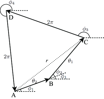
Figure 1: Planar geometric interpretation of ${\bm{m}}=0$. The vectors $\overrightarrow{\rm AB}=\theta_{2}\bm{n}(\phi_{1})$, $\overrightarrow{\rm BC}=\theta_{1}\bm{n}(\phi_{1}+\phi_{2})$, $\overrightarrow{\rm CD}=2\pi\bm{n}(\phi_{3})$ and $\overrightarrow{\rm DA}=2\pi\bm{n}(\phi_{4})$ are the summands in Eq. (17). $\theta_{1},\theta_{2}$, and $2\pi$ are the lengths of these vectors, while $\bm{n}(\phi_{i})$ indicates their directions.

Given a target $U$, the solution of $\bm{m}$ $=$ $0$ can be obtained from planar geometry (see Appendix) as

$$\phi_{3} = \pi+\phi_{1}+\phi_{2}-\arcsin\left(\frac{\theta_{2}\sin\phi_{2}}{r}\right)-\arccos\left(\frac{r}{4\pi}\right),$$

$$\phi_{4} = \pi+\phi_{3}-\arccos\left(1-\frac{r^{2}}{8\pi^{2}}\right),$$ (18)

where

$$r={\rm AC}=\sqrt{\theta_{1}^{2}+\theta_{2}^{2}+2\theta_{1}\theta_{2}\cos\phi_{2}}.$$ (19)

This is a generalization of the graphical method proposed in Odedra12 ; Jones13 .

Once a composite pulse robust against amplitude errors has been designed, simultaneous robustness to amplitude and off-resonance errors can be achieved if each of the elementary gates is replaced by a CORPSE pulseIchikawa11 ; Bando13 ; Cummins03 . This procedure is called nesting. The CORPSE pulse for the target $(\theta)_{\phi}$ is the sequence $(\theta_{3})_{\phi_{3}}(\theta_{2})_{\phi_{2}}(\theta_{1})_{\phi_{1}}$ with

$$\theta_{1} = 2n_{1}\pi+\theta/2-k,\qquad\phi_{1}=\phi,$$

$$\theta_{2} = 2n_{2}\pi-2k,\qquad\phi_{2}=\pi-\phi,$$

$$\theta_{3} = 2n_{3}\pi+\theta/2-k,\qquad\phi_{3}=\phi,$$ (20)

where $k=\arcsin[\sin(\theta/2)/2]$ and $n_{i}\in\mathbb{Z}$ $(i=1,2,3)$ satisfy a constraint $n_{1}-n_{2}+n_{3}=0$. The nesting is performed only for the constituent elementary gates that are not robust against off-resonance errors: $(2\pi)$ pulses need not to be replaced, since they already have such robustness. Thus, the sequence (12) is nested if $(\theta_{1})_{\phi_{1}+\phi_{2}}$ and $(\theta_{2})_{\phi_{1}}$ are replaced by CORPSE pulses. The resultant nested composite pulse for $\Theta$ consists of eight elementary gates.

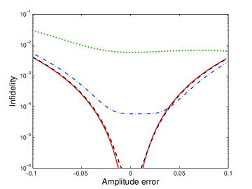
Figure 2: (Color online) Infidelity for the composite $Z_{\pi}$ gate, robust against amplitude errors, as a function of the amplitude error $\epsilon$, for a fixed off-resonance error $f$. The different fixed off-resonant errors are given by $f=0$ (solid, red), $f=0.001$ (dashed, black), $f=0.01$ (dash-dot, blue) and $f=0.1$ (dotted, green).

IV Examples

In this section, we present two examples of the composite pulse (12): the $Z_{\phi}$ and the Hadamard gates. In the subsections A and B we consider only amplitude errors. The obtained propagators are nested in subsection C to obtain simultaneous robustness against both amplitude and off-resonance errors. The robustness against both types of errors is numerically demonstrated for all examples. The robust $\Theta$ and $Z_{\phi}$ gates can implement any general robust rotation according to Eq. (10).

The robustness is calculated in terms of the infidelity between the target operation $\Theta$ and the implemented composite pulse $V^{\prime}$:

$${\cal I}=1-\frac{1}{2}|\mathrm{Tr}(\Theta^{\dagger}V^{\prime})|.$$ (21)

The robustness of the composite pulses will be shown below, observed through a small gate infidelity up to first order in amplitude and off-resonant errors.

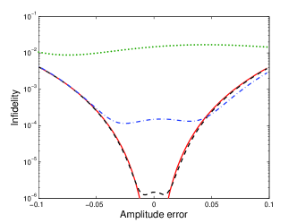
(a) (b)

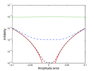
Figure 3: (Color online) Infidelity for composite Hadamard gates as a function of the amplitude error $\epsilon$, for a fixed off-resonance error $f$. (a) $\Theta=U_{H}$ based on the decomposition (25). (b) $U_{\rm H}$ based on the decomposition (26). The different fixed off-resonant errors are given by $f=0$ (solid, red), $f=0.001$ (dashed, black), $f=0.01$ (dash-dot, blue) and $f=0.1$ (dotted, green). Note that these Hadamard gates are robust only against amplitude errors.

IV.1 $Z_{\phi}$ gate

First, a robust $Z_{\phi}$ gate is constructed, employing the decomposition

$$Z_{\phi}=(\pi)_{0}(\pi)_{-\phi/2},$$ (22)

where the unphysical global phase has been ignored. Comparing the above expression with Eq. (11), $\Theta$ reads

$$\theta_{1}=\theta_{2}=\pi,\qquad\phi_{1}=0,\qquad\phi_{2}=-\phi/2.$$ (23)

Substituting them into (18) and (19), we obtain

$$\phi_{3} = \pi-\frac{\phi}{2}-\arcsin\left(\frac{-\sin(\phi/2)}{2|\cos(\phi/4)|}\right)-\arccos\frac{|\cos(\phi/4)|}{2},$$

$$\phi_{4} = \pi+\phi_{3}-\arccos\left(1-\frac{\cos^{2}(\phi/4)}{2}\right).$$ (24)

Figure 2 shows the infidelity between the target gate $\Theta=Z_{\phi}$ and the corresponding composite pulse $V^{\prime}$ with imperfect pulses.

IV.2 Hadamard gate

The composite pulses for the Hadamard gate are obtained for two different decompositions:

$$U_{\rm H} = (\pi/2)_{3\pi/2}(\pi)_{0}$$ (25)

$$= (\pi/4)_{3\pi/2}(\pi)_{0}(\pi/4)_{-3\pi/2}.$$ (26)

The latter decomposition (26) admits a symmetry with respect to the amplitude of the elementary pulse. Again, global phases are ignored.

The first decomposition (25) is directly related to $\Theta$ up to a global phase:

$$\theta_{1}=\pi,\quad\theta_{2}=\pi/2,\quad\phi_{1}=3\pi/2,\quad\phi_{2}=-3\pi/2,$$ (27)

which leads to

$$\phi_{3} = \pi-\arcsin(1/\sqrt{5})-\arccos(\sqrt{5}/8)\approx 1.39,$$

$$\phi_{4} = \pi+\phi_{3}-\arccos(27/32)\approx 3.97.$$ (28)

The infidelity is plotted in Fig. 3 (b).

To make a composite pulse with the decomposition (26), we set

$$V=(\pi/4)_{3\pi/2}(2\pi)_{\phi_{2}}(\pi)_{0}(2\pi)_{\phi_{1}}(\pi/4)_{-3\pi/2}$$ (29)

and evaluate the error vector $\bm{m}$. Since $(\theta)_{\phi}(\pi)_{0}=(\pi)_{0}(\theta)_{-\phi}$, we obtain

$$V^{\prime}=(\pi/4)_{3\pi/2}(\pi)_{0}W(\pi/4)_{-3\pi/2}$$ (30)

with

$$W=(\epsilon\pi/4)_{-3\pi/2}(2\epsilon\pi)_{-\phi_{2}}(\epsilon\pi)_{0}(2\epsilon\pi)_{\phi_{1}}(\epsilon\pi/4)_{-3\pi/2}.$$

Expanding $W$ with respect to $\epsilon$, we find

$${\bm{m}}=\pi\begin{pmatrix}2\cos\phi_{1}+2\cos\phi_{2}+1\\ 2\sin\phi_{1}-2\sin\phi_{2}+1/2\\ 0\end{pmatrix}.$$ (32)

The solution of ${\bm{m}}=0$ is

$$(\phi_{1},\phi_{2})=(\alpha,\beta),$$ (33)

where

$$\alpha = \arccos((-10-\sqrt{295})/40)\approx 2.32,$$

$$\beta = \arccos((-10+\sqrt{295})/40)\approx 1.39.$$ (34)

The infidelity is given in Fig. 3 (b). The infidelity profiles (a) and (b) are similar to those of the SK1 sequence and the symmetric-BB1 sequence, respectively Ichikawa11 . These similarities can be understood by the common feature of these composite pulses: they are constructed by inserting several $\pi$ or $2\pi$ rotations whose phases are chosen so that the resulting gate is robust against amplitude errors.

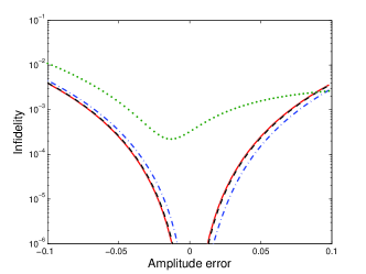
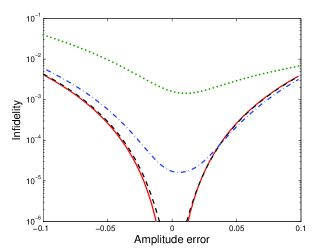
(a) (b) (c)

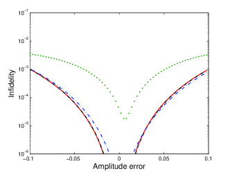
Figure 4: (Color online) Infidelity for the nested composite pulses, which have simultaneous robustness against amplitude and off-resonance errors, as a function of the amplitude error ($\epsilon$), for a fixed ORE ($f$). (a) $Z_{\pi}$ gate. (b) $\Theta=U_{H}$ based on the decomposition (25). (c) $U_{H}$ based on the decomposition (26). The different fixed off-resonant errors are given by $f=0$ (solid, red), $f=0.001$ (dashed, black), $f=0.01$ (dash-dot, blue) and $f=0.1$ (dotted, green).

IV.3 Nesting and Simultaneous Robustness

Now, the obtained composite pulses are nested so that the resulting gate is simultaneously robust against amplitude and off-resonance errors. According to the prescription in Sec. III, it is sufficient to replace the pulses in Eqs. (22), (25), and (26) with CORPSE pulses. For example, a $(\pi)_{0}$ pulse is replaced by

$$(2n_{3}\pi+\pi/3)_{0}(2n_{2}\pi-\pi/3)_{\pi}(2n_{1}\pi+\pi/3)_{0}.$$ (35)

Figure 4 shows the infidelity plots of the nested sequences. The infidelity is clearly reduced, even when $\epsilon$ and $f$ are both nonzero. The same feature has been observed for other nested pulses designed Ichikawa11 ; Bando13 .

IV.4 Comparison with other composite pulses

In order to compare different composite pulses, two important criteria are the number of elementary gates and the operation time cost of the sequence. The latter is defined by the equation

$$T=\sum_{i}\frac{|\theta_{i}|}{\pi},$$ (36)

where $\theta_{i}$ is the flip angle of the $i$-th elementary pulse. The composite pulse given in Eq. (12) has an operation time cost of $T_{\rm AE}=4+(\theta_{1}+\theta_{2})/\pi$. When nested with CORPSE pulses for simultaneous robustness, it is given by $T_{\rm nes}=12+\left[\theta_{1}+\theta_{2}-4(k_{1}+k_{2})\right]/\pi$, where $k_{i}=\arcsin[\sin(\theta_{i}/2)/2]$.

Table 1: Number of pulses, $N$, operation time cost $T$ and robustness of Hadamard and $Z_{\phi}$ gates, for different composite pulses. The last column indicates to which error type the sequence is robust, amplitude errors (AE) or off-resonance errors (ORE).

Composite pulse	Hadamard		$Z_{\phi}$		robustness
	$N$	$T$	$N$	$T$
Eq. (12)	$4$	$5.5$	$4$	$6$	AE
Eq. (29)	$5$	$5.5$	–	–	AE
SCROFULOUS	$6$	$5.3$	$6$	$6$	AE
SK1	$6$	$9.5$	$6$	$10$	AE
BB1	$8$	$9.5$	$8$	$10$	AE
nested Eq. (12)	$8$	$12.4$	$8$	$12.7$	AE, ORE
nested Eq. (29)	$11$	$16.3$	–	–	AE, ORE
reduced CinSK	$10$	$16.4$	$10$	$16.7$	AE, ORE
reduced CinBB	$12$	$16.4$	$12$	$16.7$	AE, ORE
reduced SKinsC	$12$	$12.4$	$12$	$12.7$	AE, ORE

The time cost to make a rotation robust depends on its particular decomposition and on which composite pulse is employed Bando13 . To make a comparison to the sequence of Eq. (12), $Z_{\phi}$ and Hadamard gates are decomposed as in Eqs. (22) and (25), and each rotation is replaced by a composite pulse. As it can be seen in Table 1, both gates can be implemented in a shorter time and/or smaller number of pulses if Eq. (12) is used, in comparison to other existing composite pulses. To design gates robust against amplitude errors, SK1 and BB1 sequences Brown04 ; Winperis lead to a longer execution time, while SCROFULOUS pulses Cummins03 offer a shorter one. When nested, the composite pulse of Eq. (12) has a shorter time cost in comparison to reduced CinBB and CinSK sequences, and fewer pulses than all three reduced CCCP (ConCatenated Composite Pulses Ichikawa11 ). The nested symmetric Hadamard gate of Eq. (29) also offers a slightly shorter time cost than those of CinSK and CinBB sequences.

For a general rotation, according to Eq. (10), we need to apply both $\Theta$ and $Z_{\phi}$ gates. It implies a time cost $T=24+\left[\theta_{1}+\theta_{2}-4(k_{1}+k_{2})+4\pi/3\right]/\pi$ when nested. For suppression of amplitude errors, $T=10+(\theta_{1}+\theta_{2})/\pi$. When applying other sequences, a decomposition $U=R_{x}(\alpha_{1})R_{y}(\alpha_{2})R_{x}(\alpha_{3})$ leads to a shorter time cost with all reduced CCCP, specially with reduced SKinC. For this case, $T_{\rm SKinC}=18+\left[\alpha_{1}+\alpha_{2}+\alpha_{3}-4(k_{1}+k_{2}+k_{3})\right]/\pi$. For reduced CinBB and CinSK, the execution time is of the same order as our composite pulse, $T=24+\left[\alpha_{1}+\alpha_{2}+\alpha_{3}-4(k_{1}+k_{2}+k_{3})\right]/\pi$. However, for robustness just to amplitude errors, the BB1 and SK1 pulses imply longer execution times, while SCROFULOUS attains a shorter one.

V Conclusion

In this paper, we obtained composite pulses robust against amplitude errors, which implement general one-qubit gates. Simultaneous robustness against amplitude errors and off-resonance error can be achieved using the nesting procedure. Our approach is especially useful for systems where the virtual $z$-rotation or the phase modulation techniques cannot be performed efficiently. Furthermore, the proposed sequences can improve the tolerance to these errors of any pair of sequential rotations in the $xy$-plane.

Two examples were given to illustrate our method, the phase $Z_{\phi}$ and Hadamard gates. In both cases, an expansion of the high fidelity area has been shown numerically as in Figs. 3 and 4, demonstrating the robustness of our composite pulses. A sequence symmetric in the amplitudes achieves the better performance at the cost of longer execution time. This enhancement is due to the fact that symmetries increase the robustness of pulse sequences in general Haeberlen ; JonesJMR . Moreover, using our method these two gates can be implemented with shorter execution times and smaller number of elementary pulses.

*

Appendix A Derivation of Formula (18)

Here it is shown how to solve the condition $\bm{m}=0$ to obtain Eq. (18) with the help of Fig. 1. The following relation holds at the points C and D;

$$\phi_{3}+\angle{\rm ACB}+\angle{\rm ACD}+(\pi-\phi_{1}-\phi_{2})=2\pi$$ (37)

and

$$\phi_{4}+(\pi-\phi_{3})+\angle{\rm CDA}=2\pi,$$ (38)

respectively. Thus, the problem boils down to evaluating $\angle{\rm ACB}$, $\angle{\rm ACD}$ and $\angle{\rm CDA}$. Using Eq. (19) and $\triangle$ABC in Fig. 1, we obtain

$$\angle{\rm ACB}=\arcsin\left(\frac{\theta_{2}\sin\phi_{2}}{r}\right).$$ (39)

We also find from $\triangle{\rm ACD}$ that

$$\angle{\rm ACD} = \arccos\left(\frac{r}{4\pi}\right),$$

$$\angle{\rm CDA} = \arccos\left(1-\frac{r^{2}}{8\pi^{2}}\right).$$ (40)

Substituting them into Eqs. (37) and (38), Eq. (18) is proved.

This graphical proof implies that in general two $2\pi$ pulses are necessary to make $\Theta$ robust against amplitude errors. The reason is that adding one $2\pi$ pulse cannot close the triangle when $r>2\pi$, and the error vector $\bm{m}$ does not vanish.

References

- (1) M. H. Levitt, Prog. NMR Spectrosc. 18, 61 (1986).
- (2) M. A. Nielsen and I. C. Chuang, Quantum Information and Quantum Computation, (Cambridge University Press, Cambridge, 2000).
- (3) J. Stolze and D. Suter, Quantum Computing, (Wiley-VCH, Weinheim, 2008).
- (4) M. Nakahara and T. Ohmi, Quantum Computing: From Linear Algebra to Physical Realizations (Taylor and Francis, Boca Raton, 2008).
- (5) J. A. Jones, Prog. NMR Spectrosc. 59, 91 (2011).
- (6) J. T. Merrill and K. R. Brown, arXiv:1203.6392.
- (7) N. C. Jones, R. Van Meter, A. G. Fowler, P. L. McMahon, J. Kim, T. D. Ladd and Y. Yamamoto, Phys. Rev. X 2, 031007 (2012).
- (8) X. Wang et al., Nature Comm. 3, 997 (2012).
- (9) J. P. Kestner et al., Phys. Rev. Lett. 110, 140502 (2013).
- (10) J. T. Merrill, S. C. Doret, G. D. Vittorini, J. P. Addision, K. R. Brown, arXiv:1401.1121v2 [quant-ph] (2014).
- (11) T. Ichikawa, M. Bando, Y. Kondo and M. Nakahara, Phys. Rev. A 84, 062311 (2011).
- (12) T. Ichikawa, U. Güngördü, M. Bando, Y. Kondo and M. Nakahara, Phys. Rev. A 87, 022323 (2013).
- (13) M. Bando, T. Ichikawa, Y. Kondo and M. Nakahara, J. Phys. Soc. Jpn. 82, 014004 (2013).
- (14) K. R. Brown, A. W. Harrow and I. L. Chuang, Phys. Rev. A 70, 052318 (2004).
- (15) S. Odedra, M. J. Thrippleton and S. Wimperis, J. Mag. Reson. 225, 81 (2012).
- (16) J. A. Jones, Phys. Rev. A 87, 052317 (2013).
- (17) H. K. Cummins, G. Llewellyn and J. A. Jones, Phys. Rev. A 67, 022332 (2003).
- (18) C. A. Ryan, J. S. Hodges, and D. G. Cory, Phys. Rev. Lett. 105, 200402 (2010).
- (19) Y. Kondo and M. Bando, J. Phys. Soc. Jpn. 80, 054002 (2011).
- (20) T. Ichikawa, M. Bando, Y. Kondo and M. Nakahara, Phil. Trans. R. Soc. A 370, 4671 (2012).
- (21) G. H. Low, T. J. Yoder and I. L. Chuang, Phys. Rev. A 89, 022341 (2014).
- (22) G. S. Uhrig, Phys. Rev. Lett. 98, 100504 (2007).
- (23) J. A. Jones, Phys. Lett. A 377, 2860 (2013).
- (24) Y. Makhlin, G. Schön and A. Shnirman. Rev. Mod. Phys. 73, 357 (2001).
- (25) M. I. Dykman and P. M. Platzman, Fortschr. Phys. 9-11, 1095 (2000).
- (26) See, the papers in the special issus on Jaynes-Cummings Physics of J. Phys. B: At. Mol. Opt. Phys. 46 (2013).
- (27) S. Wimperis, J. Magn. Reson. A 109, 221 (1994).
- (28) U. Haeberlen, High Resolution NMR in Solids: Selective Averaging. Advances in Magnetic Resonance. Academic Press, 1976.
- (29) S. Husain, M. Kawamura and J. A. Jones, J. Mag. Res. 230, 145 (2013).