Statistical Analysis of the Horizontal Divergent Flow in Emerging Solar Active Regions

Abstract

Solar active regions (ARs) are thought to be formed by magnetic fields from the convection zone. Our flux emergence simulations revealed that a strong horizontal divergent flow (HDF) of unmagnetized plasma appears at the photosphere before the flux begins to emerge. In our earlier study, we analyzed HMI data for a single AR and confirmed presence of this precursor plasma flow in the actual Sun. In this paper, as an extension of our earlier study, we conducted a statistical analysis of the HDFs to further investigate their characteristics and better determine the properties. From SDO/HMI data, we picked up 23 flux emergence events over a period of 14 months, the total flux of which ranges from $10^{20}$ to $10^{22}\ {\rm Mx}$. Out of 23 selected events, 6 clear HDFs were detected by the method we developed in our earlier study, and 7 HDFs detected by visual inspection were added to this statistic analysis. We found that the duration of the HDF is on average 61 minutes and the maximum HDF speed is on average $3.1\ {\rm km\ s}^{-1}$. We also estimated the rising speed of the subsurface magnetic flux to be $0.6$–$1.4\ {\rm km\ s}^{-1}$. These values are highly consistent with our previous one-event analysis as well as our simulation results. The observation results lead us to the conclusion that the HDF is rather a common feature in the earliest phase of AR emergence. Moreover, our HDF analysis has capability of determining the subsurface properties of emerging fields that cannot be directly measured.

1 Introduction

Active regions (ARs) including sunspots are one of the most prominent features in the Sun. These regions are highly magnetized and, through magnetic reconnection and instability, they may produce catastrophic eruptions known as flares and CMEs. Parker (1955) suggested that ARs are created by rising magnetic fields from the deep convection zone (flux emergence).

In the last decades, numerical simulations applying a number of different approximations have widely been carried out and they successfully explained many observational characteristics found in ARs. For instance, simulations using the thin-flux-tube approximation revealed that Coriolis force acting on the rising field is responsible for the production of AR tilts and asymmetries (D’Silva & Choudhuri, 1993; Fan et al., 1993). Emerging flux in a turbulent convective envelope was addressed employing the anelastic approximation (e.g., Jouve & Brun, 2009). However, these assumptions become inappropriate in the upper convection zone around $-20\ {\rm Mm}$ due to the drastic changes in physical parameters (Fan, 2009).

On the other hand, emergence simulations from the surface layer have elucidated the dynamical features of newly emerging flux regions. Two-dimensional magnetohydrodynamic (2D MHD) simulations by Shibata et al. (1989) reproduced the rising motion of arch filament system (AFS: Bruzek, 1969) and the supersonic downflows along the magnetic fields. Magara (2001) calculated the 2D cross-sectional evolutions of twisted flux tubes, while Fan (2001) compared her 3D simulation results with AR observation by Strous et al. (1996). 3D MHD simulations of rising, twisted flux tubes by Abbett et al. (2000) show a large, diverging horizontal flow field near the apex of the tube as it approaches the upper boundary (see, e.g., Figure 14 of that paper).

Recently, in Toriumi & Yokoyama (2012), we conducted a 3D MHD simulation of a rising magnetic flux tube in a larger scale from a depth of $-20\ {\rm Mm}$ in the convection zone, where the approximations break down, to the solar corona through the photosphere. We found that the flux tube decelerates temporarily beneath the surface of the Sun before it restarts emergence into the upper atmosphere (“two-step emergence” model). In this simulation, the flux tube goes up the solar interior at a rate of $\sim 1\ {\rm km\ s}^{-1}$ and, due to the external density and pressure stratification, it begins to expand. Moreover, because of the expansion, the tube starts to push up unmagnetized plasma on its apex. The plasma becomes trapped between the rising tube and the isothermally-stratified (i.e., convectively-stable) photosphere and, finally, it escapes horizontally around the surface layer just before the start of the flux emergence in the photosphere, which we call the horizontal divergent flow (HDF).

In Toriumi & Yokoyama (2013), we extended the above simulation and carried out a parametric survey, finding that the driving force of the HDF is the horizontal pressure gradient. We also found that the duration of the HDF (the time gap between the start of the HDF and that of the flux emergence) ranges 30–45 minutes, while the horizontal velocity is typically several km s^-1, a fraction of the photospheric sound speed ($\sim 10\ {\rm km\ s}^{-1}$). In the convective emergence simulations that solve radiative MHD, similar outflows are also observed in the earliest moments of flux emergence (Cheung et al., 2010). Rempel & Cheung (2014) reported that the flow speed reaches up to $2\ {\rm km\ s}^{-1}$.

The HDF is detected in the actual Sun. In Toriumi et al. (2012), we investigated NOAA AR 11081, which emerged closer to the northwestern limb on 2010 June 11, and found that the HDF precedes the appearance of magnetic flux. The HDF continued for 103 minutes, while its speed was $0.6$–$1.5\ {\rm km\ s}^{-1}$, up to $2.3\ {\rm km\ s}^{-1}$. These values are comparable to the simulation results, which supports the “two-step emergence” model based on the numerical experiments.

Although the previous detection is a promising result, we observed the HDF only in a single emergence event. Therefore, we need to repeat our analysis in many more events to further support the theoretical model. Also, the parameters of the HDF, such as the duration and the maximum velocity, may depend on the properties of the subsurface magnetic field that pushes up the plasma. By conducting numerical simulations of flux tube emergence, we found that these parameters actually depend on the field strength and the twist intensity of the initial flux tube (Toriumi & Yokoyama, 2013). Therefore, by analyzing HDFs in a larger ensemble of emergence events, we may be able to investigate the physical aspects of the subsurface flux such as the rising speed.

In this paper, we report on the statistical analysis of the HDFs in 23 flux emergence events. The purpose of this study is to detect HDFs in a larger ensemble of AR data and investigate their characteristics. Moreover, based on the HDF analysis, we further aim to derive any physical properties of rising magnetic fields in the solar interior. The rest of the paper is organized as follows. In the next section, we provide the data selection and reduction. In Section 3, we analyze the HDFs and show the results. Section 4 is dedicated to discussing the results and deriving the physical properties of rising flux tubes in the convection zone. Finally, in Section 5, we summarize this paper.

2 Data Selection and Reduction

2.1 Data Selection

In this study, we used observational data taken by the Helioseismic and Magnetic Imager (HMI: Scherrer et al., 2012; Schou et al., 2012) on board the Solar Dynamics Observatory (SDO). Thanks to its continual, full-disk observation, we are able to follow the AR evolution from its earliest stage. We searched for flux emergence events that occurred during the period from May 2010 to June 2011 (14 months), which is the solar minimum between Solar Cycles 23 and 24 after the launch of the SDO spacecraft in February 2010. The reason of choosing this period is to obtain “clear” events, that is, a flux emergence into quiet Sun with less preexisting magnetic fields. As the Sun steps into the active phase, it may become difficult to distinguish magnetic flux of the newly emerged fields from that of the preexisting fields, which may be the remnant of previously emerged fields. During this period, we selected emergence events in the area with a heliocentric angle $\theta\leq 60^{\circ}$ to keep the quality of HMI data. Also, we picked up only ARs that emerged in the eastern hemisphere of the solar disk in order to monitor the AR evolution as long as possible from their births. Through these criteria, we obtained 23 emergence events in 21 ARs including 2 ephemeral ARs (Harvey & Martin, 1973).

2.2 Data Reduction

For each target AR, we made tracked data cubes of the Doppler velocity and the line-of-sight (LoS) magnetogram, both having a pixel size of 0.03 heliographic degree ($\simeq 0.5\ {\rm arcsec}\simeq 360\ {\rm km}$) with a $512\times 512$ pixel field-of-view (FoV), and a 12 minute cadence with a 7 day duration. Also, for each emergence event, we made tracked data cubes of Dopplergram and LoS magnetogram with the same resolution and FoV but with a cadence of $45\ {\rm s}$ and a duration of 36 hr. For each data cube, we applied Postel projection.

In order to eliminate the effects of the rotation of the Sun and the orbital motion of the SDO spacecraft, and to reduce the east-west trend (due to the spherical geometry of the Sun) from the Dopplergram, we constructed additional background data and subtracted the background from each Doppler frame. The reduction procedure is as follows (based on the method by Grigor’ev et al. 2007).

1. To estimate the background level at the top of the FoV, we first averaged the topmost ten-pixel rows to obtain a strip of data running in the east-west direction. The strip was then linearly smoothed. We repeated the same for the bottom, to have background data with only the top and the bottom rows filled in.

2. We performed a linear interpolation between the upper and lower pixels of the columns to produce full background data.

3. By subtracting this background data from each frame, we obtained trend-free Doppler data.

In addition, a 10-minute running average was applied to the 36 hr Dopplergrams and magnetograms to smooth out rapid fluctuations that may not be related to the HDF (5-minute oscillation, surface gravity wave, etc.).

3 Analysis

3.1 Properties of ARs

In this subsection, we analyze the properties of 21 ARs. For each 7-day magnetogram of the target AR, we measured the maximum total unsigned flux, the maximum unsigned flux growth rate, and the maximum footpoint separation. In the magnetogram, we first set a box surrounding the emerging region, and measured the total unsigned flux $\Phi=\int_{S}|B|\,dS$ inside the box and its time derivative $d\Phi/dt$, where $B$ is the LoS magnetic field strength of each pixel, $S$ is the box size, $dS$ is the area of a pixel element, and $t$ is the time. We applied 120 and 240 minute smoothings for $\Phi$ and $d\Phi/dt$, respectively, and recorded their maximum values, $\max{(\Phi)}$ and $\max{(d\Phi/dt)}$. Also, within the box in each frame, we measured the flux-weighted center of each polarity

$$(x_{\pm},y_{\pm})=\left(\frac{\sum xB_{\pm}}{\sum B_{\pm}},\frac{\sum yB_{\pm}}{\sum B_{\pm}}\right),$$ (1)

where $B_{\pm}$ is the field strength of each pixel and $+$ ($-$) is for positive (negative) polarity, and evaluated the footpoint separation between both centers,

$$d_{\rm foot}=\sqrt{(x_{-}-x_{+})^{2}+(y_{-}-y_{+})^{2}}.$$ (2)

Here, for the evaluation of the flux-weighted centers, we only used the pixels with $|B|\geq 200\ {\rm G}$ to keep the data quality. Then, we recorded the maximum separation, $\max{(d_{\rm foot})}$.

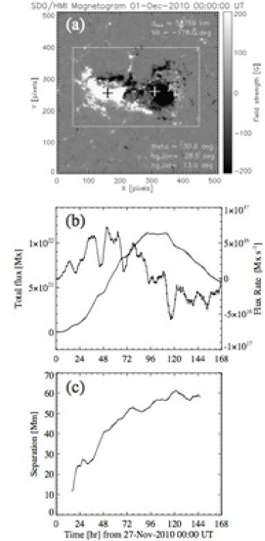
Figure 1: An example of AR data from the list in Appendix A. (a) HMI magnetogram of NOAA AR 11130 (event #7). Black and white crosses are the flux-weighted centers of positive and negative polarities, respectively, which are calculated inside the rectangular box. (b) Temporal evolutions of the total unsigned flux ($\Phi$: thick) and its time derivative ($d\phi/dt$: thin). (c) Temporal evolution of the footpoint separation ($d_{\rm foot}$).

Figure 1 is an example of AR data. In panel (a), the HMI magnetogram of NOAA AR 11130 (event #7) is shown and the flux-weighted center of each polarity is indicated with a cross sign. Panel (b) is for the temporal evolutions of the total unsigned flux ($\Phi$) and the flux growth rate ($d\Phi/dt$). One interesting characteristic of this figure is the several peaks in the flux rate curve, which may indicate that the emerging flux is bifurcated and consists of separate flux bundles (Zwaan, 1985). Panel (c) shows the footpoint separation ($d_{\rm foot}$). The maximum total flux, the maximum flux rate, and the maximum separation of this AR are $1.1\times 10^{22}\ {\rm Mx}$, $7.3\times 10^{16}\ {\rm Mx\ s}^{-1}$, and $61.1\ {\rm Mm}$, respectively. The corresponding figures of all the analyzed ARs are listed in Appendix A.

The obtained properties of the target regions are summarized in Table 1. As can be seen in this table, the total flux ranges from $5.6\times 10^{20}$ to $2.3\times 10^{22}\ {\rm Mx}$, while the flux growth rate ranges from $1.3\times 10^{16}$ to $1.7\times 10^{17}\ {\rm Mx\ s}^{-1}$ and the footpoint separation ranges from $20.5$ to $89.3\ {\rm Mm}$. Note that, in order to keep the data quality, the physical values of each AR in this table are measured under the condition that the heliocentric angle is $\theta\leq 60^{\circ}$. We should also take care of the fact that, because of the diffusion of the sunspots, footpoint separations of some ARs may become larger even after the ARs complete their growths. Regarding quadrupolar regions such as NOAA AR 11158 (event #16), we measure the separation not between the most distant footpoints but between the two representative flux-weighted centers simply calculated from the entire AR.

3.2 Detection of the HDF

First, for each 36 hr data of the 23 emergence events, we measured the start of the HDF in the Dopplergram (HDF start: $t_{\rm HDF}$) and the start of the flux emergence in the LoS magnetogram (emergence start: $t_{\rm FE}$). Here, we used the method developed in Toriumi et al. (2012): We plotted the histograms of the Doppler velocity and the absolute LoS magnetic field strength inside the square that surrounds the emergent area. By focusing on the residuals of the histograms from their reference quiet-Sun profiles, i.e., the histograms before the emergence, we investigated the temporal evolutions of the Doppler and magnetic fields. The HDF start (emergence start) was determined as the time when the high-speed component of the Doppler residual (strongly-magnetized component of the magnetic residual) exceeded the one standard deviation ($1\sigma$) level of the reference profile. For the details of the method, see Section 3.2 of Toriumi et al. (2012). In the present study, we used the square of the size of $64\times 64$ pixels ($\sim 23\ {\rm Mm}\times 23\ {\rm Mm}$). The ranges for the high-speed and strongly-magnetized components depend on the emergence event, typically being [$-1.5\ {\rm km\ s}^{-1}$, $-1\ {\rm km\ s}^{-1}$] and [$1\ {\rm km\ s}^{-1}$, $1.5\ {\rm km\ s}^{-1}$] for the Dopplergram and [$200\ {\rm G}$, $300\ {\rm G}$] for the magnetogram.

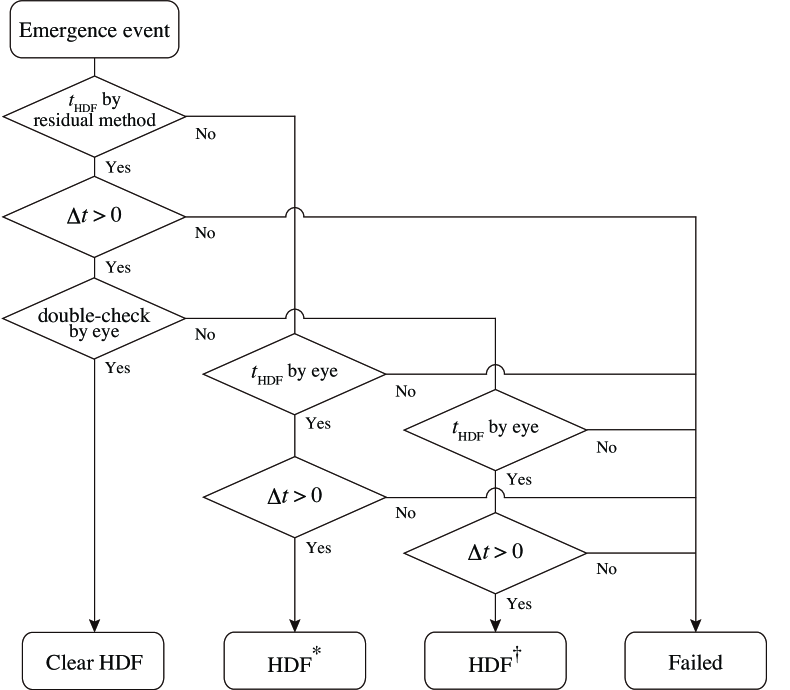
Figure 2: Flowchart of the HDF detection. Here, $t_{\rm HDF}$ and $t_{\rm FE}$ denote the HDF start and the emergence start, respectively, while $\Delta t=t_{\rm FE}-t_{\rm HDF}$. In every event, $t_{\rm FE}$ is determined and thus this process is not shown in the chart.

The analysis procedure of the HDF detection is shown as a flowchart in Figure 2. Since in every emergence event we were able to determine $t_{\rm FE}$ using the above residual method, we skipped this process in the chart. In this procedure, if $t_{\rm HDF}$ was once defined by the residual method, we then calculated the time gap between these two times (HDF duration: $\Delta t=t_{\rm FE}-t_{\rm HDF}$). If $\Delta t>0$, we double-checked the Doppler images by visual inspection and determined if the HDF was clear (clear HDF) or not. If $\Delta t\leq 0$, we defined that the HDF detection was failed. If $t_{\rm HDF}$ was not defined by the residual method, we determined $t_{\rm HDF}$ by visual inspection and, again, if $\Delta t>0$, we defined that the HDF was detected (HDF by eye: indicated with asterisk). If the result of the double-check was negative, we also determined $t_{\rm HDF}$ by eye and checked if $\Delta t>0$ (HDF by eye: indicated with dagger).

The results of the detection are shown in Table 2. In 6 emergence events out of the entire 23 events, we observed clear HDFs, that is, $t_{\rm HDF}$ was detected by the residual method, satisfied $\Delta t>0$, and passed the double-check process. The temporal evolutions of the Dopplergram and magnetogram for the 6 clear events, along with the corresponding continuum images, are shown in Figure 8 in Appendix B. In another 7 events, we detected HDFs by visual inspection instead of the residual method. Thus, in total, HDFs were found in 13 events, or, 56.5% of all the analyzed events.

In the 6 clear events, the HDF duration $\Delta t$ ranges from 5 to 106 minutes (the average $61.0$ minutes and the median $56.0$ minutes). For these events, we also evaluated the maximum horizontal speed from the Doppler velocity, $V_{\rm D}$. During $\Delta t$, we applied a slit with a thickness of 5 pixels to the Dopplergrams and averaged over 5 pixels, and measured the largest absolute Doppler velocity. Here, the slit is parallel to the separation of both magnetic polarities, centered at the middle of the emergent region. Using the heliocentric angle $\theta$, the maximum horizontal velocity can be obtained by

$$\max{(|V_{\rm h}|)}=\frac{\max{(|V_{\rm D}|)}}{\sin{\theta}}.$$ (3)

Table 3 shows the results of this analysis. The maximum HDF speed ranges from $1.8$ to $4.4\ {\rm km\ s}^{-1}$ (the average $3.1\ {\rm km\ s}^{-1}$ and the median $3.4\ {\rm km\ s}^{-1}$). The obtained durations and the horizontal speeds will be discussed in Section 4.2.

4 Discussion

4.1 HDF Detection

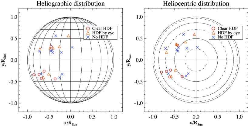
Figure 3: Distribution of the flux emergence events. (Left) Heliographic coordinates, where the Sun’s rotation axis is fixed onto the $x$–$y$ plane. (Right) Heliocentric coordinates, where the LoS is perpendicular to the $x$–$y$ plane, i.e., $z$-axis is toward the Earth.

In the previous section, we analyzed 23 flux emergence events and detected 6 clear HDFs. Also, we found 7 more HDFs by visual inspection. Figure 3 shows the distribution of the events in heliographic and heliocentric coordinates. From the heliographic map, one may find that newly emerging ARs are distributed in the mid-latitude bands of both hemispheres (latitude ranging approximately from $\pm 15^{\circ}$ to $\pm 30^{\circ}$). Also, from the heliocentric map, one can see that all clear HDFs are detected in the range of $\theta>30^{\circ}$.

In the remaining 10 events, we did not find HDFs. The possible reasons for the failed detections are as follows.

• If the flux emergence occurs at the location too close to the disk center, the HDF may not appear in the Dopplergrams because of the projection. In fact, all 6 clear events are located away from the disk center ($\theta>30^{\circ}$), while 7 out of 10 failed events are closer to the center ($\theta\leq 30^{\circ}$).

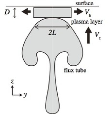
Figure 4: 2D cross-sectional model of a rising flux tube and a plasma layer ahead of the tube. Figure reproduced from Toriumi & Yokoyama (2013).

• The HDF may be stronger in the direction of the separation of the positive and negative polarities (see, e.g., Figure 4 of Toriumi & Yokoyama, 2012). When the footpoint separation on the solar disk is perpendicular to the axis from the disk center to the target AR, the HDF may not be seen, since it has less Doppler component. This effect seems to be responsible for the failed detection in event #11.

• The smaller ARs may not have coherency or energy enough to push up the sufficient amount of plasma that can be observed as HDF. In the two ephemeral ARs (events #8 and #21), we did not observe HDFs in both cases.

• If the flux emerges into a preexisting field, it is difficult to separate the HDF from the Doppler component caused by the preexisting field (event #23).

4.2 Comparison with Numerical Models

For the 6 clear HDF events, we observed that the HDF duration is on average 61 minutes. This value is comparable to the duration of 103 minutes previously measured in Toriumi et al. (2012). This value is also consistent with 30–45 minutes obtained from a parameter survey of the flux emergence simulations in Toriumi & Yokoyama (2013). According to the simulations, the HDF duration is comparable to the elapse time from the deceleration of the rising flux at the top convection zone to the start of further emergence into the upper atmosphere. In other words, the time gap of 61 minutes indicates the waiting time for the secondary emergence in the “two-step emergence” model (Section 1). Note that, in the actual Sun, thermal convection is continuously excited around the surface layer and thus the situation may be more complex.

The maximum HDF speed of the 6 clear events is on average $3.1\ {\rm km\ s}^{-1}$, which is again comparable to $2.3\ {\rm km\ s}^{-1}$ obtained in the previous observation (Toriumi et al., 2012). According to our simulation (Toriumi & Yokoyama, 2013), the HDF is driven by the pressure gradient and the maximum velocity is several km s^-1, which agrees with the present observation results. In the convective emergence simulation, such a horizontally-diverging flow is also seen in the earliest phase of the flux emergence (Cheung et al., 2010). According to the simulation by Rempel & Cheung (2014), the flow speed is up to $2\ {\rm km\ s}^{-1}$, which is comparable to our observation of $3.1\ {\rm km\ s}^{-1}$.

4.3 Investigation of the Subsurface Magnetic Fields

In this section, we investigate the subsurface rising magnetic fields that push up the unmagnetized plasma, which is observed as an HDF.

First, we consider a simple 2D model of the emerging magnetic flux as illustrated in Figure 4. Here, we assume that the rising speed of the magnetic flux $V_{z}$ is of the order of Alfvén speed $V_{\rm A}$ (Parker, 1975), namely,

$$V_{z}=\alpha V_{\rm A}=\alpha\frac{B}{\sqrt{4\pi\rho}},$$ (4)

where $B$ and $\rho$ are the field strength and the plasma density. For simplicity, we here assume the factor $\alpha$ to be unity. From the mass conservation of the HDF, we obtain

$$V_{\rm h}=\frac{L}{D}V_{z}=\frac{L}{D}\frac{B}{\sqrt{4\pi\rho}},$$ (5)

where $V_{\rm h}$, $L$, and $D$, are the horizontal speed, the lateral extension, and the thickness of the HDF, respectively. Also, the flux growth rate when the flux appears at the surface can be written as:

$$\frac{d\Phi}{dt}=2LV_{z}B=2L\frac{B^{2}}{\sqrt{4\pi\rho}},$$ (6)

where $\Phi$ is the magnetic flux. Combining Equations (5) and (6), we get

$$V_{\rm h}=\frac{(L/2)^{1/2}}{D(4\pi\rho)^{1/4}}\left[\frac{d\Phi}{dt}\right]^{1/2}.$$ (7)

In this equation, the horizontal speed $V_{\rm h}$ and the flux growth rate $d\Phi/dt$ can be measured from the observational data, which are summarized in Table 3.

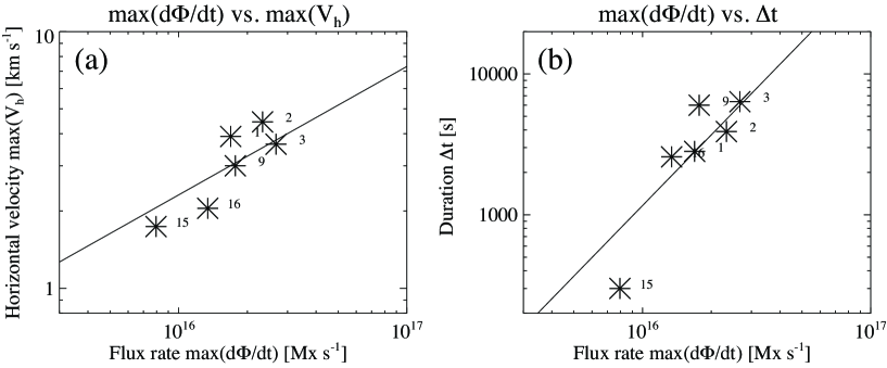
Figure 5: (a) Maximum flux growth rate, $\max{(d\Phi/dt)}$, and maximum horizontal speed, $\max{(V_{\rm h})}$, for the 6 clear HDF events. The solid line is the fitted function $\max{(V_{\rm h})}=C_{1}\times[\max{(d\Phi/dt)}]^{1/2}$. (b) Maximum flux growth rate, $\max{(d\Phi/dt)}$, and HDF duration, $\Delta t$, for the 6 clear HDF events. The solid line is the fitted function $\Delta t=C_{2}\times[\max(d\Phi/dt)]^{C_{3}}$. In both panels, the number right to each asterisk represents the event number.

In Figure 5(a), we plot $\max{(d\Phi/dt)}$ and $\max{(V_{\rm h})}$, measured during $\Delta t$, for the 6 clear HDF events. Here, we fit a function $\max{(V_{\rm h})}=C_{1}\times[\max{(d\Phi/dt)}]^{1/2}$ in the diagram. The obtained constant $C_{1}$ is comparable to the coefficient in Equation (7). The result of the fitting is

$$C_{1}=\frac{(L/2)^{1/2}}{D(4\pi\rho)^{1/4}}=2.3\times 10^{-3}.$$ (8)

In the fitting process, $V_{\rm h}$ is measured in the unit of ${\rm cm\ s}^{-1}$. From Equation (8), by assuming $L=5\ {\rm Mm}$ and $\rho=2.5\times 10^{-7}\ {\rm g\ cm}^{-3}$, we obtain the thickness of the HDF, $D=1.6\ {\rm Mm}$.

Finally, by inserting $D=1.6\ {\rm Mm}$ into Equation (5), the rising speed of the magnetic flux, $V_{z}$, is evaluated for each HDF event, which is summarized in the rightmost column of Table 3. The rising speed of the magnetic flux ranges from $0.6$ to $1.4\ {\rm km\ s}^{-1}$. This value is comparable to our simulation results of $\sim 1\ {\rm km\ s}^{-1}$ in Toriumi & Yokoyama (2013) and other simulations of the flux emergence within the convection zone (see Fan, 2009). This obtained speed is also comparable to the helioseismic detections of rising magnetic fields (e.g., Ilonidis et al., 2011; Toriumi et al., 2013).

Figure 5(b) shows the relation between the maximum flux growth rate, $\max{(d\Phi/dt)}$, and the HDF duration, $\Delta t$. According to Equation (6), $d\Phi/dt$ is proportional to the square of $B$. The linear trend in Figure 5(b) is the fitted function $\Delta t=C_{2}\times[\max(d\Phi/dt)]^{C_{3}}$ and the best fitting parameters are $C_{2}=2.7\times 10^{-24}$ and $C_{3}=1.7$. Thus, the observation indicates $\Delta t\propto B^{3.4}$. In the parameter survey of the flux emergence simulations (see Figure 4 of Toriumi & Yokoyama, 2013), we found that, when the initial tube is stronger (field strength $\gtrsim 30\ {\rm kG}$), the HDF duration $\Delta t$ is inversely proportional to the field strength of the initial flux tube at a depth of $-20\ {\rm Mm}$. On the other hand, when the tube is weaker (field strength $\lesssim 30\ {\rm kG}$), it deviates from the inverse variation and has a positive correlation with the field strength. Therefore, the observed positive correlation of $\Delta t\propto B^{3.4}$ hints that the field strength of the rising flux in the deeper convection zone ($\sim-20\ {\rm Mm}$) has a field strength of $\lesssim 30\ {\rm kG}$.

4.4 Correlation with AR Parameters

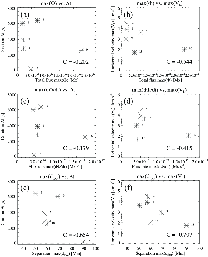
Figure 6: Correlations between HDF parameters (HDF duration, $\Delta t$, and maximum HDF speed, $\max{(V_{\rm h})}$) and AR parameters (maximum total unsigned flux, $\max{(\Phi)}$, maximum flux rate, $\max{(d\Phi/dt)}$, and maximum footpoint separation, $\max{(d_{\rm foot})}$). Correlation coefficient $C$ is indicated in the bottom right of each panel. Note that these parameters are measured from the 7-day magnetograms, under the condition of $\theta\leq 60^{\circ}$.

Figure 6 summarizes the correlations between HDF parameters (HDF duration, $\Delta t$, and maximum HDF speed, $\max{(V_{\rm h})}$) and AR parameters (maximum total unsigned flux, $\max{(\Phi)}$, maximum flux rate, $\max{(d\Phi/dt)}$, and maximum footpoint separation, $\max{(d_{\rm foot})}$) for 6 clear HDF events. Note that the AR parameters including $\max{(d\Phi/dt)}$ were measured not during the HDF duration (i.e., $\Delta t$) but during the entire AR evolution using 7-day magnetogram. The measurement is limited by the condition that the heliocentric angle, $\theta$, is $\leq 60^{\circ}$ (see Section 3.1).

In this figure, the best correlation is $-0.7$ of panel (f), the correlation between the maximum footpoint separation, and the maximum HDF speed. According to the simulation results of Toriumi & Yokoyama (2013), the maximum HDF speed is proportional to the initial field strength (see Figure 4(c) of that paper). On the other hand, when the field is stronger, the total flux is expected to be larger, and thus the AR size, or, the footpoint separation may also become larger. Therefore, the maximum separation and the maximum horizontal speed are expected to have a positive correlation. However, the observational result of Figure 6(f) is totally opposite from this expectation. The absolute correlation coefficients of other panels are at most, or less than $0.6$. The AR parameters here represent the global structure of emerging magnetic flux that eventually forms the AR, and, since the HDF appears only in the very initial phase of the flux emergence, the correlation with the HDF parameters may not be so high.

4.5 HDF and Elongated Granules

In continuum, the granulation pattern in an emerging flux region is known to appear different from that in quiet Sun. In the early phase of flux emergence, the transient dark alignments, or the darkened intergranular lanes, appear in the center of the emerging region, aligned roughly in parallel with the axis connecting the two main polarities (Brants & Steenbeek, 1985; Zwaan, 1985; Strous & Zwaan, 1999). It is thought that the dark lanes are created by the horizontal magnetic fields at the apex of the rising flux tube from the convection zone (Zwaan, 1985). Numerical simulations also support this scenario (e.g., Cheung et al., 2007)

In event #1 in Figure 8, for example, the granulation pattern in the continuum image looks mostly circular at first at 07:15 UT and also at 07:30 UT, namely, after the HDF start ($t_{\rm HDF}=$ 07:24 UT). However, at 08:00 UT, the pattern in the central region shows a slight elongation to the direction of the red and blue Doppler pair. Although the flux emergence is not detected yet by the residual method at this moment ($t_{\rm FE}=$ 08:11 UT), the magnetogram shows a faint positive (white) pattern, which may be the horizontal magnetic fields reflected because of the projection (this emerging AR is located 46.5^∘ away from the disk center). However, at 08:15 UT, namely, after the significant LoS flux is detected at 08:11 UT, the elongated pattern is not seen in the continuum. This transient elongation reminds us of the concept that the HDF is pushed up by the horizontal magnetic fields at the apex of the large-scale rising flux transported from the deep convection zone, which agrees well with the “two-step emergence” scenario.

5 Summary

In this paper, we have shown a statistical analysis of newly emerging ARs. In the numerical simulations of the “two-step emergence” model (e.g., Toriumi & Yokoyama, 2012), when the flux approaches the solar surface, unmagnetized plasma becomes trapped between the rising flux and the photosphere and eventually escapes horizontally around the surface layer. This HDF was previously detected in a single emergence event in Toriumi et al. (2012) and, in the present study, we extended the detection in many more events, aiming to investigate the characteristics of the HDF.

Under the conditions of (1) the solar minimum, (2) $\theta\leq 60^{\circ}$, and (3) the eastern hemisphere, we picked up 23 flux emergence events in 21 ARs, total unsigned flux ranging from $5.6\times 10^{20}$ to $2.3\times 10^{22}\ {\rm Mx}$. Using the method developed in Toriumi et al. (2012), we detected 6 clear HDFs. In another 7 emergence events, we found HDFs by visual inspection. In total, the HDFs were observed in 56.6% of all events. If we exclude the emergence events closer to the disk center ($\theta\leq 30^{\circ}$), which are supposed to have less Doppler components, the detection rate increases up to more than 80%.

In the 6 clear events, the HDF duration from the HDF appearance to the flux emergence was on average 61 minutes, which is consistent with 103 minutes observed in the previous detection (Toriumi et al., 2012) and 30–45 minutes obtained in the numerical experiments (Toriumi & Yokoyama, 2013). According to the simulations, this time gap is comparable to the waiting time after the rising magnetic flux slows down in the top convection zone before it restarts emergence into the upper atmosphere. The maximum horizontal speed of the HDF in the present study is on average $3.1\ {\rm km\ s}^{-1}$, which is also consistent with $2.3\ {\rm km\ s}^{-1}$ observed in the previous detection (Toriumi et al., 2012) and several ${\rm km\ s}^{-1}$ in the simulations (Toriumi & Yokoyama, 2013).

Assuming a simple 2D model, we estimated the rising speed of the subsurface magnetic flux that pushes up and drives the HDF. The estimated rising speed was $0.6$–$1.4\ {\rm km\ s}^{-1}$, which is again consistent with the simulations (Toriumi & Yokoyama, 2013), previous calculations of the emergence in the solar interior (e.g., Fan, 2009), and other seismic studies (e.g., Toriumi et al., 2013). By comparing with the simulation results in Toriumi & Yokoyama (2013), we also speculated that the rising flux tubes have a field strength of less than $30\ {\rm kG}$ in the deeper convection zone at around $-20\ {\rm Mm}$.

On the other hand, it was found that the correlations between HDF parameters (the duration and the flow speed) and AR parameters (the total flux, its time derivative, and the footpoint separation) are not so high. This may be because, while the AR parameters represent the global structure of the rising magnetic fields, the HDF parameters are more focused on the initial phase of the flux emergence, or the apex of the rising fields. We also observed the transient elongation of granular cells after the HDF was detected in the emerging region. Since the elongated structure reflects the horizontal field around the surface layer, this observation is also in good agreement with the “two-step emergence” scenario.

In this analysis, by comparing the temporal evolutions of the magnetic and velocity distributions with their reference quiet-Sun profiles, we succeeded in detecting the HDF signatures. By visual inspection, the HDF is easy to distinguish from other convections such as granulation and supergranulation (as in Doppler images in Figure 8). It is because, although the typical size of the HDF is about the same as that of supergranulation ($\sim 10$–$20\ {\rm Mm}$), the horizontal speed is larger than that of the supergranulation (HDF $\sim 1.5\ {\rm km\ s}^{-1}$; supergranulation $\sim$ a few $100\ {\rm m\ s}^{-1}$). Moreover, although the HDF velocity is comparable to the granulation speed ($0.5$–$1.5\ {\rm km\ s}^{-1}$), the size scale is by far different (granulation $\sim 0.5$–$2\ {\rm Mm}$). Given the above characteristics of the HDF signatures, together with our method that compares with the reference quiet-Sun profiles, one can see that the strong flows detected in this study are not occurring by chance. For obtaining better statistical significance of the HDF detection and its quantification, we can utilize the full-disk Dopplergrams in our future study to expand the analyzed region so as not to miss, if any, HDF events without being associated with magnetic field emergence in the quiet-Sun regions.

In this paper, we statistically analyzed the HDFs in a larger ensemble of emerging AR data. We conclude here that the HDF is a rather common feature in the earliest phase of AR-scale flux emergence. We also found that the obtained HDF parameters are highly consistent with the numerical results and the previous detection. Moreover, the HDF observation provides us with a tool to investigate the physical states of the subsurface magnetic fields.

Appendix A List of Target ARs

Figure 7 is a list of target ARs analyzed in this study. Here, we show the HMI magnetogram, the temporal evolutions of the total unsigned flux $\Phi$ and its time derivative (flux growth rate) $d\Phi/dt$, and the footpoint separation $d_{\rm foot}$ between the two polarities. The definition of each value is shown in Section 3.1. In the magnetogram, we also show the flux-weighted centers of positive and negative polarities with cross signs. The flux and the centroids are measured within the overlaid box. Note that the physical values of events #22 and #23 are not measured because of the overlapping with each other.

Appendix B Clear HDF Events

Figure 8 shows the temporal evolution of 6 clear HDF events (events #1, #2, #3, #9, #15, and #16) observed by SDO/HMI. Each column shows the HMI continuum image, Dopplergram, and magnetogram. The overlaid square indicates the area in which we plot the histogram for the determination of the HDF start $t_{\rm HDF}$ and the emergence start $t_{\rm FE}$.

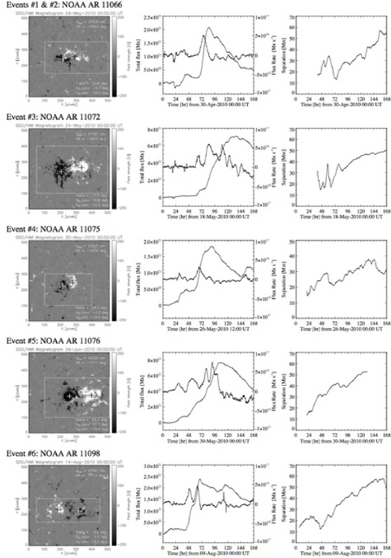
Figure 7: ARs analyzed in this study. (Left) SDO/HMI magnetogram. Footpoint separation ($d_{\rm foot}$), tilt angle, heliocentric angle ($\theta$), heliographic latitude and longitude at the shown time are indicated. Black and white crosses denote the flux-weighted centers of the positive and negative polarities, respectively, which are measured within the box. (Middle) Temporal evolution of the total unsigned flux ($\Phi$: thick) and its time derivative ($d\Phi/dt$: thin). (Right) Footpoint separation ($d_{\rm foot}$).

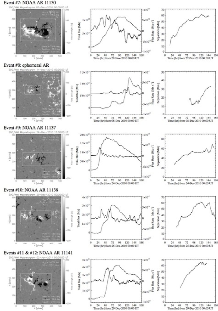
Figure 7: Continued.

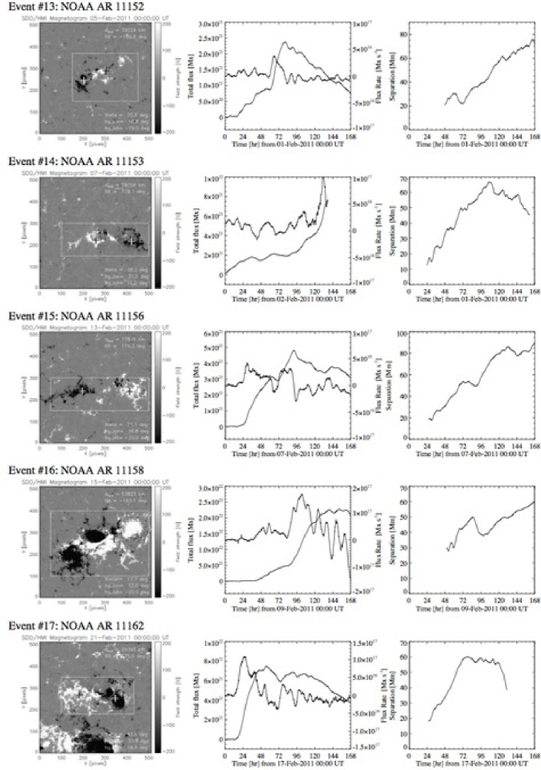
Figure 7: Continued.

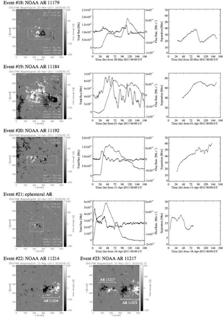
Figure 7: Continued.

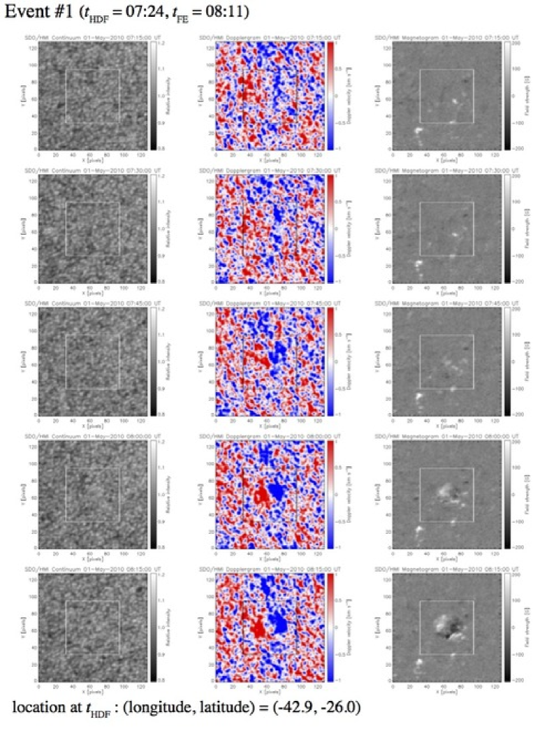
Figure 8: Clear HDF events. Left, middle, and right columns show the evolutions of the continuum image, Dopplergram, and magnetogram, respectively. The square indicates the area in which we plot the histogram for the determination of the HDF start and the emergence start.

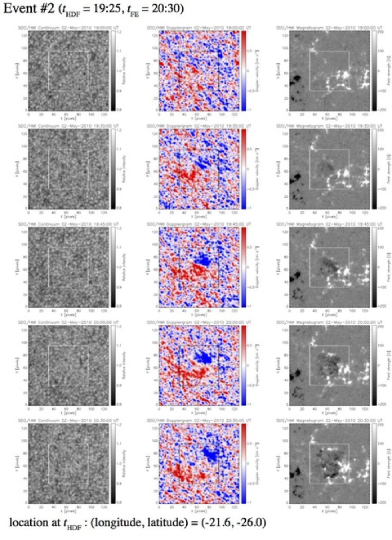
Figure 8: Continued.

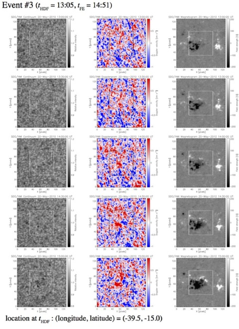
Figure 8: Continued.

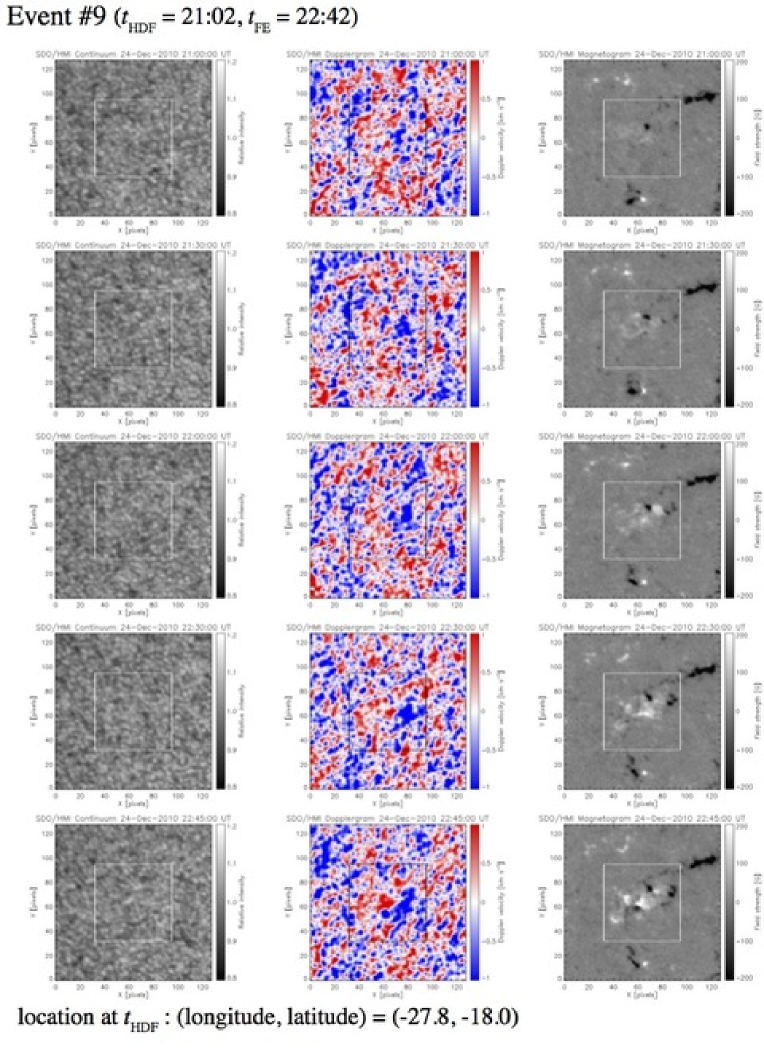
Figure 8: Continued.

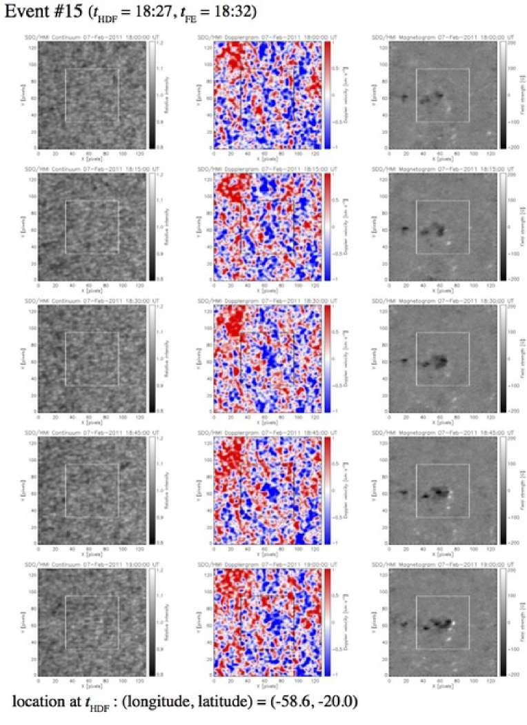
Figure 8: Continued.

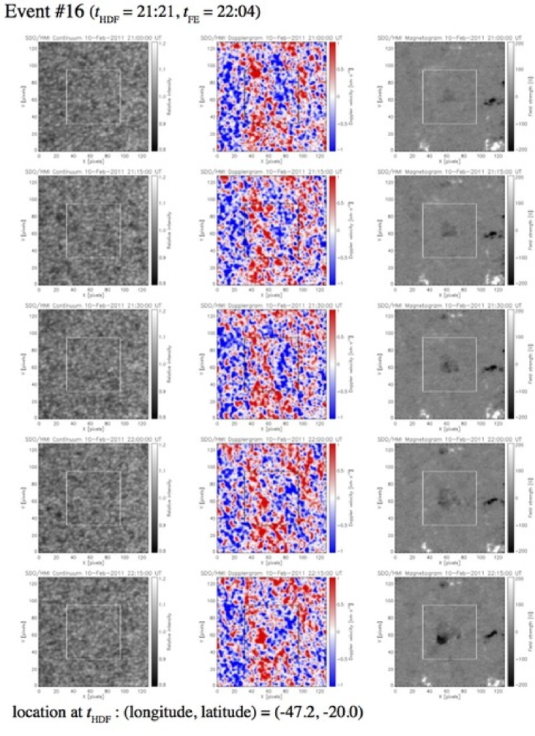
Figure 8: Continued.

Table 1: Newly emerging ARs analyzed in this study.

Event #	NOAA AR #	Year	Date	$\max{(\Phi)}$	$\max{(d\Phi/dt)}$	$\max{(d_{\rm foot})}$
				(Mx)	(Mx s-1)	(Mm)
1	11066	2010	May 1	$2.1\times 10^{21}$	$5.1\times 10^{16}$	$57.1$
2	”		May 2	”	”	”
3	11072		May 20	$7.1\times 10^{21}$	$6.0\times 10^{16}$	$50.1$
4	11075		May 27	$1.8\times 10^{21}$	$3.3\times 10^{16}$	$38.0$
5	11076		May 30	$7.7\times 10^{21}$	$7.5\times 10^{16}$	$52.9$
6	11098		Aug 10	$2.4\times 10^{21}$	$4.7\times 10^{16}$	$57.9$
7	11130		Nov 27	$1.1\times 10^{22}$	$7.3\times 10^{16}$	$61.1$
8	ephemeral		Dec 10	$1.2\times 10^{21}$	$2.6\times 10^{16}$	$32.6$
9	11137		Dec 24	$1.8\times 10^{21}$	$3.9\times 10^{16}$	$68.3$
10	11138		Dec 26	$3.1\times 10^{21}$	$4.4\times 10^{16}$	$61.4$
11	11141		Dec 29	$4.3\times 10^{21}$	$6.1\times 10^{16}$	$64.8$
12	”		Dec 30	”	”	”
13	11152	2011	Feb 1	$2.4\times 10^{21}$	$3.8\times 10^{16}$	$75.7$
14	11153		Feb 2	$7.7\times 10^{21}$	$1.1\times 10^{17}$	$66.8$
15	11156		Feb 7	$4.8\times 10^{21}$	$4.2\times 10^{16}$	$89.3$
16	11158		Feb 10	$2.3\times 10^{22}$	$1.7\times 10^{17}$	$59.6$
17	11162		Feb 17	$7.5\times 10^{21}$	$1.1\times 10^{17}$	$60.1$
18	11179		Mar 20	$1.9\times 10^{21}$	$3.1\times 10^{16}$	$38.2$
19	11184		Apr  2	$8.2\times 10^{21}$	$8.7\times 10^{16}$	$72.8$
20	11192		Apr 12	$1.6\times 10^{21}$	$3.6\times 10^{16}$	$59.8$
21	ephemeral		Apr 18	$5.6\times 10^{20}$	$1.3\times 10^{16}$	$20.5$
22	11214		May 13	–	–	–
23	11217		May 15	–	–	–

Table 2: Results of the HDF detection.

Event #	NOAA AR #	Year	Date	$t_{\rm HDF}$	$t_{\rm FE}$	$\Delta t$	HDF	$\theta$
						(min)		(∘)
1	11066	2010	May  1	07:24	08:11	47	Y	46.5
2	”		May  2	19:25	20:30	65	Y	30.1
3	11072		May 20	13:05	14:51	106	Y	40.6
4	11075		May 27	–	05:59	–	N	45.7
5	11076		May 30	17:08	16:31	$-37$	N	35.7
6	11098		Aug 10	(18:40)	19:36	56	Y∗	45.4
7	11130		Nov 27	–	06:54	–	N	28.0
8	ephemeral		Dec 10	–	11:00	–	N	17.2
9	11137		Dec 24	21:02	22:42	100	Y	33.6
10	11138		Dec 26	10:21	07:49	$-152$	N	29.7
11	11141		Dec 29	–	13:44	–	N	41.3
12	”		Dec 30	(19:15)	20:08	53	Y∗	36.7
13	11152	2011	Feb  1	(16:41)	16:58	52	Y†	32.7
14	11153		Feb  2	(21:38)	21:36	33	Y†	35.7
15	11156		Feb  7	18:27	18:32	5	Y	58.2
16	11158		Feb 10	21:21	22:04	43	Y	47.4
17	11162		Feb 17	(14:15)	15:04	49	Y∗	29.2
18	11179		Mar 20	–	22:02	–	N	29.6
19	11184		Apr  2	(00:40)	02:21	101	Y∗	36.7
20	11192		Apr 12	02:48	01:19	$-89$	N	19.9
21	ephemeral		Apr 18	–	02:13	–	N	49.0
22	11214		May 13	(13:00)	14:26	77	Y†	43.6
23	11217		May 15	–	07:29	–	N	25.7

Table 3: Clear HDF events.

Event #	$\Delta t$	$\theta$	$\max(|V_{\rm D}|)$	$\max(|V_{\rm h}|)$	$\max(d\Phi/dt)$	$V_{z}$
	(min)	(∘)	(km s-1)	(km s-1)	(Mx s-1)	(km s-1)
1	47	46.5	2.8	3.9	$1.4\times 10^{16}$	1.3
2	65	30.1	2.2	4.4	$2.1\times 10^{16}$	1.4
3	106	40.6	2.4	3.7	$1.1\times 10^{16}$	1.2
9	100	33.6	1.7	3.1	$9.4\times 10^{15}$	1.0
15	5	58.2	1.5	1.8	$1.2\times 10^{16}$	0.6
16	43	47.4	1.5	2.0	$3.0\times 10^{15}$	0.7

References

- Abbett et al. (2000) Abbett, W. P., Fisher, G. H., & Fan, Y. 2000, ApJ, 540, 548
- Brants & Steenbeek (1985) Brants, J. J., & Steenbeek, J. C. M. 1985, Sol. Phys., 96, 229
- Bruzek (1969) Bruzek, A. 1969, Sol. Phys., 8, 29
- Cheung et al. (2010) Cheung, M. C. M., Rempel, M., Title, A. M., & Schüssler, M. 2010, ApJ, 720, 233
- Cheung et al. (2007) Cheung, M. C. M., Schüssler, M., & Moreno-Insertis, F. 2007, A&A, 467, 703
- D’Silva & Choudhuri (1993) D’Silva, S., & Choudhuri, A. R. 1993, A&A, 272, 621
- Fan (2001) Fan, Y. 2001, ApJ, 554, L111.
- Fan et al. (1993) Fan, Y., Fisher, G. H., & DeLuca, E. E. 1993, ApJ, 405, 390
- Fan (2009) Fan, Y. 2009, Living Reviews in Solar Physics, 6, 4
- Frazier (1972) Frazier, E. N. 1972, 26, 130
- Grigor’ev et al. (2007) Grigor’ev, V. M., Ermakova, L. V., & Khlystova, A. I. 2007, Astronomy Letters, 33, 766
- Harvey & Martin (1973) Harvey, K. L., & Martin, S. F. 1973, Sol. Phys., 32, 389
- Ilonidis et al. (2011) Ilonidis, S., Zhao, J., & Kosovichev, A. 2011, Science, 333, 993
- Jouve & Brun (2009) Jouve, L., & Brun, A. S. 2009, ApJ, 701, 1300
- Magara (2001) Magara, T. 2001, ApJ, 549, 608
- Parker (1955) Parker, E. N. 1955, ApJ, 121, 491
- Parker (1975) Parker, E. N. 1975, ApJ, 198, 205
- Rempel & Cheung (2014) Rempel, M., & Cheung, M. C. M. 2014, ApJ, 785, 90
- Scherrer et al. (2012) Scherrer, P. H. et al. 2012, Sol. Phys., 275, 207
- Schou et al. (2012) Schou, J. et al. 2012, Sol. Phys., 275, 229
- Shibata et al. (1989) Shibata, K., Tajima, T., Steinolfson, R. S., & Matsumoto, R. 1989, ApJ, 345, 584
- Strous et al. (1996) Strous, L. H., Scharmer, G., Tarbell, T. D., Title, A. M., & Zwaan, C. 1996, A&A, 306, 947
- Strous & Zwaan (1999) Strous, L. H., & Zwaan, C. 1999, ApJ, 527, 435
- Toriumi (2014) Toriumi, S. 2014, PhD thesis, The University of Tokyo
- Toriumi et al. (2013) Toriumi, S., Ilonidis, S., Sekii, T., & Yokoyama, T. 2013, ApJ, 770, L11
- Toriumi et al. (2012) Toriumi, S., Hayashi, K., & Yokoyama, T. 2012, ApJ, 751, 154
- Toriumi & Yokoyama (2012) Toriumi, S., & Yokoyama, T. 2012, A&A, 539, A22
- Toriumi & Yokoyama (2013) Toriumi, S., & Yokoyama, T. 2013, A&A, 553, A55
- Zwaan (1985) Zwaan, C. 1985, Sol. Phys., 100, 397