On the Role of Pseudodisk Warping and Reconnection in Protostellar Disk Formation in Turbulent Magnetized Cores

Abstract

The formation of rotationally supported protostellar disks is suppressed in ideal MHD in non-turbulent cores with aligned magnetic field and rotation axis. A promising way to resolve this so-called “magnetic braking catastrophe” is through turbulence. The reason for the turbulence-enabled disk formation is usually attributed to the turbulence-induced magnetic reconnection, which is thought to reduce the magnetic flux accumulated in the disk-forming region. We advance an alternative interpretation, based on magnetic decoupling-triggered reconnection of severely pinched field lines close to the central protostar and turbulence-induced warping of the pseudodisk of Galli and Shu. Such reconnection weakens the central split magnetic monopole that lies at the heart of the magnetic braking catastrophe under flux freezing. We show, through idealized numerical experiments, that the pseudodisk can be strongly warped, but not completely destroyed, by a subsonic or sonic turbulence. The warping decreases the rates of angular momentum removal from the pseudodisk by both magnetic torque and outflow, making it easier to form a rotationally supported disk. More importantly, the warping of the pseudodisk out of the disk-forming, equatorial plane greatly reduces the amount of magnetic flux threading the circumstellar, disk-forming region, further promoting disk formation. The beneficial effects of pseudodisk warping can also be achieved by a misalignment between the magnetic field and rotation axis. These two mechanisms of disk formation, enabled by turbulence and field-rotation misalignment respectively, are thus unified. We find that the disks formed in turbulent magnetized cores are rather thick and significantly magnetized. Implications of these findings, particularly for the thick young disk inferred in L1527, are briefly discussed.

1 Introduction

How disks form is a longstanding, unsolved problem in star formation (Bodenheimer 1995). Observationally, it has been difficult to determine when and how the disks first come into existence during the star formation process. Although disks are routinely observed around evolved Class II young stellar objects (see Williams & Cieza 2011 for a review) and increasingly around younger Class I sources (e.g., Brinch et al. 2007; Jørgensen et al. 2009; Lee 2011; Takakuwa et al. 2012; Harsono et al. 2014; Lindberg et al. 2014), observations of the youngest disks have been hampered by the emission from their massive envelope. Nevertheless, rotationally supported disks are beginning to be detected around deeply embedded, Class 0 protostars (Tobin et al. 2012; Murillo et al. 2013; N. Ohashi, priv. comm.). This impressive observational progress is expected to accelerate in the near future, as ALMA becomes fully operational.

Theoretically, disk formation is complicated by magnetic fields, which are observed in dense, star-forming, cores of molecular clouds (see Crutcher 2012 for a review). In the simplest case of a non-turbulent core with the magnetic field aligned with the rotation axis, both analytic considerations and numerical simulations have shown that the formation of a rotationally supported disk (RSD hereafter) is suppressed, in the ideal MHD limit, by a realistic magnetic field (corresponding to a dimensionless mass-to-flux ratio of $\lambda\sim$ a few; Troland & Crutcher 2008) during the protostellar mass accretion phase through magnetic braking (Allen et al. 2003; Galli et al. 2006; Price & Bate 2007; Mellon & Li 2008; Hennebelle & Fromang 2008; Dapp & Basu 2010; Seifried et al. 2011; Santos-Lima et al. 2012). This suppression of RSDs is termed the “magnetic braking catastrophe.”

There are a number of mechanisms proposed in the literature to overcome the catastrophic braking, including (1) non-ideal MHD effects (ambipolar diffusion, the Hall effect and Ohmic dissipation), (2) misalignment between the magnetic and rotation axes, and (3) turbulence (see Li et al. 2014 for a critical review of the proposed mechanisms). Ambipolar diffusion does not appear to weaken the braking enough to enable large-scale RSD formation under realistic conditions (Krasnopolsky & Königl 2002; Mellon & Li 2009; Duffin & Pudritz 2009; Li et al. 2011). Ohmic dissipation can produce small, AU-scale, RSDs in the early protostellar accretion phase (Machida et al. 2011; Dapp & Basu 2010; Dapp et al. 2012; Tomida et al. 2013). How such disks grow in time remain to be fully quantified. Larger, $10^{2}{\rm\,{\rm AU}}$-scale RSDs can be produced if the resistivity or the Hall coefficient of the dense core is much larger than the classical (microscopic) value (Krasnopolsky et al. 2010; Krasnopolsky et al. 2011; Santos-Lima et al. 2012; Braiding & Wardle 2012a; Braiding & Wardle 2012b). Large RSDs can also form if the magnetic field is misaligned with the rotation axis by a large angle (see Hull et al. 2013 for observational evidence for misalignment but Davidson et al. 2011 and Chapman et al. 2013 for evidence to the contrary), provided that the dense core is not too strongly magnetized (Joos et al. 2012; Li et al. 2013; Krumholz et al. 2013).

The effects of turbulence on magnetized disk formation were first explored by Santos-Lima et al. (2012), who demonstrated that a strong enough turbulence can enable the formation of a $10^{2}{\rm\,{\rm AU}}$-scale RSD. The beneficial effects of turbulence on disk formation were confirmed numerically by a number of authors, including Seifried et al. (2012, 2013), Santos-Lima et al. (2013), Myers et al. (2013), and Joos et al. (2013). However, why the turbulence is conducive to disk formation remains hotly debated. Santos-Lima et al. (2012, 2013) attributed the disk formation to the turbulence induced or enhanced magnetic reconnection (Lazarian & Vishniac 1999; Kowal et al. 2009), which reduces the strength of the magnetic field in the inner, disk-forming, part of the accretion flow. Seifried et al. (2012, 2013) proposed instead that the turbulence-induced tangling of field lines and strong local shear are mainly responsible for the disk formation: the disordered magnetic field weakens the braking and the shear enhances rotation. Joos et al. (2013) found that the turbulence produced an effective magnetic diffusivity that enabled the magnetic flux to diffuse outward, broadly consistent with the picture envisioned in Santos-Lima et al. (2012, 2013). It also generated a substantial misalignment between the rotation axis and magnetic field direction (an effect also seen in Seifried et al. 2012 and Myers et al. 2013), which is known to promote disk formation. The lack of consensus on why turbulence helps disk formation in magnetized cloud cores motivated us to examine this important issue more closely.

We carry out numerical experiments of disk formation in magnetized dense cores with different levels of initial turbulence. We find that the magnetic flux threading the circumstellar, disk-forming region on the equatorial plane is indeed reduced by turbulence. We show that this reduction can be explained by a combination of magnetic decoupling-triggered reconnection of severely pinched field lines close to the central object and a simple geometry effect — warping of the well-known magnetic pseudodisk (Galli & Shu 1993) out of the disk-forming, equatorial plane by turbulence — without having to rely on turbulence-induced magnetic reconnection. We find that the turbulence-induced pseudodisk warping also reduces the rates of angular momentum removal by both magnetic torque and outflow, which is conducive to disk formation. We describe the problem setup in § 2. The numerical results are presented and analyzed in § 3. We compare our results to previous work and discuss their implications in § 4 and conclude with a summary in § 5.

2 Problem Setup

We will adopt the basic setup of Santos-Lima et al. (2012; see also Krasnopolsky et al. 2010), where a rotating, magnetized, turbulent but non-self-gravitating dense core accretes onto a central object of fixed mass. This setup is idealized, but has an important advantage for our purpose of understanding why turbulence helps disk formation in a magnetized core. It enables us to repeat the type of calculations by Santos-Lima et al. (2012), but at a better spatial resolution in the disk-forming region (and a lower numerical diffusivity for the magnetic field). The higher resolution is achieved using the ZeusTW code (Krasnopolsky et al. 2010), which can follow the core collapse and disk formation on a non-uniform grid in a spherical polar coordinate system. This coordinate system is more natural than the Cartesian coordinate system for disk formation simulations, especially for implementing clean boundary conditions near the accreting protostar for both the matter and magnetic field (see § 2.2 of Mellon & Li 2008 and discussion below). Our goal is to develop a qualitative understanding based on simple numerical experiments. Quantitative results may be modified when self-gravity is included (see discussion in § 4.4).

Following Li et al. (2011) and Krasnopolsky et al. (2012), we start our simulations from a uniform, spherical core of $1{\rm\,{\rm M_{\odot}}}$ and radius $R_{0}=10^{17}{\rm\,{\rm cm}}$ in a spherical coordinate system $(r,\theta,\phi)$. The initial density $\rho_{0}=4.77\times 10^{-19}{\rm\,{{\rm g}{\rm\,{\rm cm}}^{-3}}}$ corresponds to a molecular hydrogen number density of $10^{5}{\rm\,{\rm cm}}^{-3}$. We adopt an isothermal equation of state with a sound speed $a=0.2{\rm\,{{\rm km}{\rm\,{\rm s}}^{-1}}}$ below a critical density $\rho_{c}=10^{-13}{\rm\,{{\rm g}{\rm\,{\rm cm}}^{-3}}}$, and a polytropic equation of state $p\propto\rho^{5/3}$ above it. Following Krasnopolsky et al. (2010), we adopt the following prescription for the initial rotation speed:

$$v_{\phi}=v_{\phi,0}\tanh(\varpi/\varpi_{c}),$$ (1)

which implies that the equatorial plane is the plane of disk formation. We adopt $v_{\phi,0}=2\times 10^{4}{\rm\,{{\rm cm}{\rm\,{\rm s}}^{-1}}}$ and $\varpi_{c}=3\times 10^{15}{\rm\,{\rm cm}}$ to ensure that a large, well resolved, rotationally supported disk is formed at a relatively early time in the absence of any magnetic braking (see Fig. 1 of Krasnopolsky et al. 2010 and Fig. 19 below). The goal of our numerical experiments is to determine whether such a disk is suppressed by a realistic level of magnetic field in the absence of turbulence and, if yes, whether turbulence can weaken the magnetic braking enough to allow the disk to reappear.

Since the focus of our investigation is on the effects of turbulence, we will consider only one value, $B_{0}=35.4{\rm\,{\mu\rm G}}$, for the strength of the magnetic field, which is assumed to be uniform initially and aligned with the rotation axis (i.e., with a misalignment angle $\theta_{0}=0^{\circ}$; a misaligned case of $\theta_{0}=90^{\circ}$ will be discussed in § 4). It corresponds to a dimensionless mass-to-flux ratio $\lambda=2.92$, in units of the critical value $(2\pi G^{1/2})^{-1}$, for the core as a whole, which is not far from the median value of $\lambda\sim 2$ inferred by Troland & Crutcher (2008) for a sample of nearby dense cores. The mass-to-flux ratio for the central flux tube $\lambda_{c}$ is higher than the global value $\lambda$ by $50\%$, so that $\lambda_{c}=4.38$. Our chosen magnetic field is therefore not unusually strong; if anything, it may be on the weak side.

We add a turbulent velocity field to the magnetized core at the beginning of the simulation. Although the existence of “turbulence” on the $0.1{\rm\,{\rm pc}}$ core scale has been known for a long time through “non-thermal” linewidth (e.g., Myers 1995), its detailed properties, such as energy spectra, remain poorly constrained observationally. For simplicity, we generate the initial turbulent velocity field as a superposition of 1000 sinusoidal waves of wavelengths logarithmically spaced between a minimum wavelength $l_{\min}=2\times 10^{14}{\rm\,{\rm cm}}$ and a maximum $l_{\max}=5\times 10^{16}{\rm\,{\rm cm}}$. The initial velocity vector of each sinusoidal wave has an amplitude that is proportional to $l^{p}$, a random phase, and a random direction that is perpendicular to an equally random wave propagation vector. We have experimented with different number of waves and random seeds, and found qualitatively similar results. The main parameter that we decide to vary is the level of turbulence, which is characterized by the rms Mach number $M$. In § 3, we will discuss in some depth six models that have the same turbulent velocity field except for the overall normalization, which is given respectively by $M=0$ (non-turbulent, Model A of Table 1), $0.1$ (Model B), $0.3$ (Model C), $0.5$ (Model D), $0.7$ (Model E), and $1$ (Model F). In addition, we will consider the disk formed in a non-magnetic, non-turbulent core (Model H) and a case with the magnetic field orthogonal to the rotation axis ($\theta_{0}=90^{\circ}$, Model P), for comparison with the disks formed in the aligned ($\theta_{0}=0^{\circ}$) case that are enabled by turbulence (see § 4).

Table 1: Models

Model	$\lambda^{\rm a}$	$M$	$p$	$\theta_{0}$	RSDb
A	2.92	0.0	N/A	0∘	No
B	2.92	0.1	1	0∘	No
C	2.92	0.3	1	0∘	No
D	2.92	0.5	1	0∘	Yes/Transient
E	2.92	0.7	1	0∘	Yes/Transient
F	2.92	1.0	1	0∘	Yes/Persistent
H	$\infty$	0.0	N/A	0∘	Yes/Persistent
P	2.92	0.0	N/A	90∘	Yes/Persistent
U	2.92	1.0	0.5	0∘	Yes/Persistent
V	2.92	1.0	2.0	0∘	Yes/Persistent

Note. — (a) The average dimensionless mass-to-flux ratio for the core as a whole. (b) “Persistent” disks are rotationally supported structures that rarely display large deviations from smooth Keplerian motions, whereas “transient” disks are highly active, rotationally dominated structures with large distortions and are often completely disrupted.

We choose a non-uniform grid of $120\times 90\times 90$. In the radial direction, the inner and outer boundaries are located at $r=10^{14}$ and $10^{17}{\rm\,{\rm cm}}$, respectively. The radial cell size is smallest near the inner boundary ($5\times 10^{12}{\rm\,{\rm cm}}$ or $\sim 0.33{\rm\,{\rm AU}}$). It increases outward by a constant factor $\sim 1.06$ between adjacent cells. In the polar direction, we choose a relatively large cell size ($5{{}^{\circ}}$) near the polar axes, to prevent the azimuthal cell size from becoming prohibitively small in the polar region; it decreases smoothly to a minimum of $\sim 0.52{{}^{\circ}}$ near the equator, where rotationally supported disks may form. The grid is uniform in the azimuthal direction. Our finest cell in the disk-forming equatorial region has dimensions of $0.33$, $0.07$, and $0.47{\rm\,{\rm AU}}$ in the $r$-, $\theta$-, and $\phi$-direction, respectively. This is comparable to that of Joos et al. (2013, $0.4{\rm\,{\rm AU}}$), and better than those of Seifried et al. (2012, $1.2{\rm\,{\rm AU}}$), Myers et al. (2013, $10{\rm\,{\rm AU}}$), and Santos-Lima et al. (2012, $15.6{\rm\,{\rm AU}}$). The higher resolution should reduce the level of numerical diffusion of magnetic field and its associated reconnection, especially compared to that in Santos-Lima et al. (2012), whose results we seek to verify and understand physically. Our non-uniform grid is shown in Fig. 1. It was designed to provide good resolution for the disk forming equatorial region. Half of our radial cells lie within a radius of $\sim 200{\rm\,{\rm AU}}$, and half of our polar cells within $\sim 20^{\circ}$ of the equatorial plane. For example, the relatively thick disk shown in Fig. 21 below contains about $2.5\times 10^{5}$ cells.

Figure 1: Computational grid in the meridian plane, showing good resolution in the disk-forming equatorial region.

The boundary conditions in the azimuthal direction are periodic. In the radial direction, we impose the standard outflow boundary conditions for both the hydrodynamic quantities and magnetic field, at both the inner and outer boundaries. The boundary conditions are enforced using ghost zones. For the density and three components of the velocity, we simply copy their values in the active zone closest to the boundary into the ghost zones, except when the radial component of the velocity is pointing into the computation domain (i.e., $v_{r}>0$ near the inner boundary or $v_{r}<0$ near the outer boundary); in such cases, the radial velocity is set to zero in the ghost zones to prevent mass flowing into the computation domain from outside, where there is no self-consistently determined flow information. These boundary conditions allow matter and angular momentum to leave the outer radial boundary, as needed for the magnetic-braking driven outflow, and to accrete through the inner radial boundary. The boundary conditions on the magnetic field are enforced through the electromotive force (EMF), which is used to evolve the field everywhere, including the ghost zones, using the method of constrained transport (CT). The three components of the EMF are copied from the active zone closest to the boundary into the ghost zones. In effect, we are assuming continuity from the computation domain into the ghost zones for both the hydrodynamic quantities and magnetic field, which minimizes the risks of artificial wave reflection at the boundary. The use of CT ensures that the divergence-free condition $\nabla\cdot{\bf B}=0$ is preserved to machine accuracy in both the active computation domain and the ghost zones. In particular, the magnetic field lines dragged by the accretion flow across the inner boundary stay on the boundary, forming essentially a split magnetic monopole, as expected in ideal MHD (Galli et al. 2006), until (numerical) reconnection is triggered by severe pinching of the oppositely directed field lines (see Mellon & Li 2008 and discussion below). The radius of our inner boundary is $10^{14}{\rm\,{\rm cm}}$ (or $6.7{\rm\,{\rm AU}}$). It is larger than the sink accretion radius used by Seifried et al. (2013, $3{\rm\,{\rm AU}}$) but smaller than that of Santos-Lima et al. (2012, $62.5{\rm\,{\rm AU}}$). Since our inner boundary is covered by nearly 10,000 cells, it can resolve the angular distributions of the magnetic field and flow quantities better than the “sink accretion region” of Santos-Lima et al. (2012) and Seifried et al. (2013). We note that there was formally no “sink accretion region” in Joos et al. (2013). They adopted a stiffened equation of state above a mass density of $10^{-13}{\rm\,{{\rm g}{\rm\,{\rm cm}}^{-3}}}$, which produced an artificially thermally supported object of order $10{\rm\,{\rm AU}}$ in size (comparable to that of our inner boundary), which served as an effective “inner boundary” for their simulations. Note that their “inner boundary” is quite different from the “sink accretion region” of Santos-Lima et al. (2012) and Seifried et al. (2013), and both treatments are very different from ours. How these different treatments affect the numerical results remains to be quantified.

On the polar axes, the boundary condition is chosen to be reflective. Although this is not strictly valid, we expect its effect to be limited to a small region near the axis. As in Krasnopolsky et al. (2010) and Santos-Lima et al. (2012), the central point mass is fixed at $0.5{\rm\,{\rm M_{\odot}}}$.

Although it is desirable to carry out the simulations in ideal MHD, so that they can be compared more directly with other works, especially Santos-Lima et al. (2012), we found the ideal MHD simulations difficult to perform in practice, because they tend to produce numerical “hot zones” where the Courant conditions demand such a small timestep that they force the calculation to stop early, a tendency we noted in our previous 2D (Mellon & Li 2008) and 3D simulations (Krasnopolsky et al. 2012 and Li et al. 2013). To lengthen the simulation, we include a small, spatially uniform resistivity $\eta=10^{17}{\rm\,{{\rm cm}^{2}{\rm\,{\rm s}}^{-1}}}$. We have verified that, in Model F with $M=1$ (which turns out to be one of the most interesting cases and will be discussed in greatest detail), this resistivity changes the flow structure little compared to either the ideal MHD limit or a model where the resistivity is reduced by a factor 10, to $10^{16}{\rm\,{{\rm cm}^{2}{\rm\,{\rm s}}^{-1}}}$, at early times (before the non-resistive and low-resistivity runs stop). It is at least two orders of magnitude smaller than the value needed to enable large-scale disk formation by itself (Krasnopolsky et al. 2010).

There was no mention of the need for using explicit resistivity to lengthen simulation of magnetized disk formation by other groups. The exact reason for this difference is unclear, although we suspect that it is related to the relatively low magnetic diffusivity in our code from the use of (1) fixed non-uniform grid, which avoids the numerical diffusion associated with refinement and derefinement, and (2) method of characteristics in constrained transport, which makes the MHD algorithm more accurate (Stone & Norman 1992). The results of the current simulations from different groups appear to depend strongly on the numerical code used in each study. In the future, it will be desirable to benchmark all MHD codes used for disk formation simulations against common test problems such as the collapse of a non-rotating, uniformly magnetized sphere of constant density, especially in the protostellar accretion phase, when the magnetic field is severely pinched and its structure is sensitive to the level of numerical diffusivity (see related discussion in footnote 2 below).

3 Numerical Results and Analysis

3.1 Turbulence-Enabled Disk Formation

To illustrate the effects of turbulence on disk formation in magnetized dense cores, we carried out a set of six simulations with identical initial conditions except for the level of turbulence, which is characterized, respectively, by the rms turbulent Mach number $M=0$, $0.1$, $0.3$, $0.5$, $0.7$, and $1$ (see Models A–F in Table 1). The simulations were run to a common final time $t=1.1\times 10^{12}{\rm\,{\rm s}}$ or about $3.5\times 10^{4}$ years. Fig. 2 shows the density distribution and velocity field on the equatorial plane at a representative time $t=8\times 10^{11}{\rm\,{\rm s}}$ for all six cases. The difference in morphology is striking.

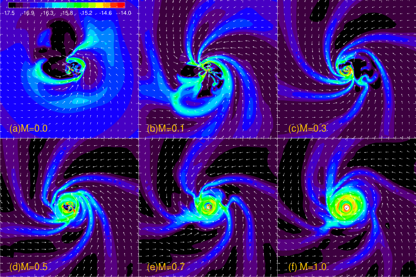
Figure 2: Density distribution and velocity field on the equatorial plane at a representative time ($t=8\times 10^{11}{\rm\,{\rm s}}$) for models with different levels of turbulence (Model A–F). The beneficial effect of turbulence on disk formation is evident. Each panel is $2\times 10^{16}{\rm\,{\rm cm}}$ on the side. The color bar is for the logarithm of the density added to a floor value of $10^{-17.5}{\rm\,{{\rm g}{\rm\,{\rm cm}}^{-3}}}$. Equatorial values taken at a latitude between $0$ and $0.26{{}^{\circ}}$.

In the non-turbulent ($M=0$) model (Model A), there is no hint of any rotationally supported disk (RSD), consistent with previous work. The circumstellar region is dominated by a highly magnetized, low-density expanding region (the so-called “decoupling enabled magnetic structure” or DEMS that has been discussed extensively in Zhao et al. 2011 and Krasnopolsky et al. 2012; see Fig. 7 and § 3.3 below). This behavior is not changed fundamentally by a modest amount of turbulence in the $M=0.1$ (Model B) or $0.3$ (Model C) cases, where the RSD remains suppressed and DEMS remains dynamically important. Here, the turbulence does change the appearance of the density distribution on the equatorial plane drastically. It produces well-ordered dense spirals that are absent in the non-turbulent case. The spirals mark the locations where a thin, warped, pseudodisk (shown in Figs. 9 and 10 below) intercepts the equatorial plane.

The apparent spirals persist as the level of turbulence increases. At the time shown in Fig. 2, they appear to merge into a disk-like structure in Model D ($M=0.5$), although the central region of the structure is still filled with low-density “holes.” This porous disk is highly dynamic. It forms around $\sim 6\times 10^{11}{\rm\,{\rm s}}$, and becomes disrupted by $\sim 9\times 10^{11}{\rm\,{\rm s}}$ (a movie illustrating the transient nature of the disk is available online as auxiliary material). The situation is similar in the slightly stronger turbulence case of $M=0.7$ (Model E), where a transient disk is also formed. Compared to the $M=0.5$ case, the disk in the $M=0.7$ case forms earlier ($\sim 2\times 10^{11}{\rm\,{\rm s}}$), and lasts longer (until $\sim 9.5\times 10^{11}{\rm\,{\rm s}}$). As the level of turbulence increases to $M=1$ (Model F), a well-defined disk forms earlier still ($\sim 10^{11}{\rm\,{\rm s}}$), grows steadily with time, and persists to the end of the simulation. As seen from Fig. 3, the disk is rotationally supported, with an average rotation speed close to the Keplerian speed and a much smaller infall speed inside a radius of $\sim 2\times 10^{15}{\rm\,{\rm cm}}$ at the time shown in Fig. 2 ($t=8\times 10^{11}{\rm\,{\rm s}}$). This is in contrast with the non-turbulent case (Model A) where the rotation on the same $100{\rm\,{\rm AU}}$ scale is highly sub-Keplerian and is dominated by infall. The rotationally supported disk in Model F turns out to be rather thick and significantly magnetized. Its properties will be discussed in more detail in § 4. Here we focus on the unmistakable trend that a stronger turbulence leads to the formation of a more robust disk. The question is: why is the disk formation suppressed in the non-turbulent or weakly turbulent cases but enabled by a stronger turbulence?

Figure 3: Mass-weighted infall (lower two curves) and rotation (upper two) speed as a function of radius for the non-turbulent (Model A, solid curves) and sonic turbulence (Model F, dashed) cases. The averaging is done within $20^{\circ}$ of the equatorial plane. A Keplerian profile (dotted line) is shown for comparison.

One possibility is that a stronger turbulence may increase the initial angular momentum by a larger amount, making it easier to form a RSD. However, even in the most turbulent case of Model F, the increase is modest, by $\sim 10\%$ or less over most of the mass (and volume; see Fig. 4). It is unlikely that such a modest change alone can explain the drastically different outcomes for our non-turbulent and sonic turbulence cases.

Figure 4: The ratio of the initial angular momenta enclosed within a sphere as a function of the mass enclosed within the same sphere for the sonic turbulence (Model F) and non-turbulent (Model A) cases, showing that in these cases the turbulence increases the initial angular momentum by about $10\%$ or less over most of the mass (and volume). The mass is normalized to $1{\rm\,{\rm M_{\odot}}}$.

3.2 Obstacle to Disk Formation: Central Split Magnetic Monopole

Disk suppression in ideal MHD is conceptually tied to another fundamental problem in star formation — the so-called “magnetic flux problem.” If the field lines in a dense core magnetized to the observed level are dragged by collapse into the central stellar object, they would produce a split magnetic monopole near the center that is strong enough to remove essentially all of the angular momentum of the accreted material and prevent the formation of a rotationally supported circumstellar disk (Galli et al. 2006). However, it is well known that if the flux freezing holds strictly during the core collapse, the stellar field strength would be orders of magnitude above the observed values (Shu et al. 1987). This magnetic flux problem must be resolved one way or another, and its resolution is a prerequisite for disk formation.

The stellar magnetic flux problem can be resolved in principle through non-ideal MHD effects (e.g., Li & McKee 1996; Contopoulos et al. 1998; Kunz & Mouschovias 2010; Machida et al. 2011; Dapp & Basu 2010; Dapp et al. 2012; Tomida et al. 2013), which decouple the field lines from the matter at high densities close to the central object. In ideal MHD simulations, the decoupling can be mimicked by numerically induced magnetic flux redistribution. To demonstrate that flux redistribution has indeed occurred in our simulations, we plot in Fig. 5 the magnetic flux $\Phi_{r}$ that leaves the surface of a sphere of radius $r$:

$$\Phi_{r}(r)=\int B_{r}(>0)\ dS$$ (2)

where the integration is over the part of the surface with magnetic field pointing outward, i.e., $B_{r}>0$ (we have verified that the amount of flux entering the sphere is exactly the same as that going out). Near the inner boundary $r_{i}=10^{14}{\rm\,{\rm cm}}$, this flux provides a measure of the strength of the central split magnetic monopole. Its value on any sphere is to be compared with the magnetic flux expected to be dragged into the same sphere by matter under the condition of flux freezing, $\Phi_{r,\rm ff}$. The expected flux depends on the amount of mass that has already accumulated inside the sphere ($M(r)$, including the mass that has passed through the inner boundary), and whether the mass is accumulated along or across the field lines; mass accumulation along field lines would not lead to any flux increase. In the limit that all of the mass along the field lines that initially thread a sphere has accumulated inside the sphere, the expected flux would be

$$\Phi_{r,\rm ff}^{\min}(r)=\pi B_{0}R_{0}^{2}\left\{1-\left[1-\frac{M(r)}{M_{\rm tot}}\right]^{2/3}\right\},$$ (3)

where $B_{0}$, $R_{0}$ and $M_{\rm tot}=\frac{4\pi}{3}\rho_{0}R_{0}^{3}$ are the initial field strength, radius, and total mass of the core. This flux is a (generous) lower limit to $\Phi_{r,\rm ff}$ at relatively small radii, where only a small fraction of the mass along any given field line has collapsed close to the central object at the relatively early times under consideration. It is derived by relating the magnetic flux $\Phi$ enclosed within a cylinder of radius $\varpi$ in the initially constant-density dense core with a uniform magnetic field to the mass enclosed by the same cylinder. An upper limit to $\Phi_{r,\rm ff}$ is obtained by assuming that the mass accumulation is isotropic, which yields

$$\Phi_{r,\rm ff}^{\max}(r)=\pi B_{0}R_{0}^{2}\left[\frac{M(r)}{M_{\rm tot}}\right]^{2/3}.$$ (4)

This is an upper limit because the core collapse proceeds somewhat faster along field lines than across.

Figure 5: Total outgoing magnetic flux $\Phi_{r}$ threading a sphere (defined in equation 2, in units of ${\rm G}{\rm\,{\rm cm}}^{2}$) as a function of the radius of the sphere for the non-turbulent case (Model A, $M=0$, solid line) and sonic turbulence case (Model F, $M=1$, dashed) at time $t=8\times 10^{11}{\rm\,{\rm s}}$ (same as Fig. 2). Also plotted for comparison are an upper (top dotted line) and lower (bottom dotted) limit to the magnetic flux expected under the flux freezing condition, given by equations (4) and (3), respectively, for Model A.

From Fig. 5, it is clear that the actual magnetic flux $\Phi_{r}$ is below the minimum value $\Phi_{r,\rm ff}^{\min}$ expected from flux-freezing at small radii ($r\lesssim 4\times 10^{14}{\rm\,{\rm cm}}$). This is evidence for magnetic flux redistribution, which has reduced the flux near the inner boundary (and hence the strength of the split magnetic monopole) by at least a factor of 4 (more likely an order of magnitude) in the non-turbulent case (Model A, solid line in the figure). The flux redistribution is likely related to a similar behavior that Mellon & Li (2008) observed in their 2D (axisymmetric) self-gravitating simulations. They found episodic reconnection of the oppositely directed field lines above and below the equatorial plane near the inner boundary (see their Fig. 16). We have carried out several 2D (axisymmetric) non-self-gravitating simulations with different spatial resolutions and different values of resistivity $\eta$ (including $\eta=0$), and found episodic reconnection in all cases. Movies of two examples are included as online auxiliary material, and their snapshots at a representative time $t=8\times 10^{11}{\rm\,{\rm s}}$ (or frame 80) are shown in Fig. 6. They have the same initial mass and magnetic field distributions as Models A–F but with $\eta=0$ and without any initial rotation, and have inner radius $r_{i}=10^{14}$ and $1.5\times 10^{13}{\rm\,{\rm cm}}$, respectively.

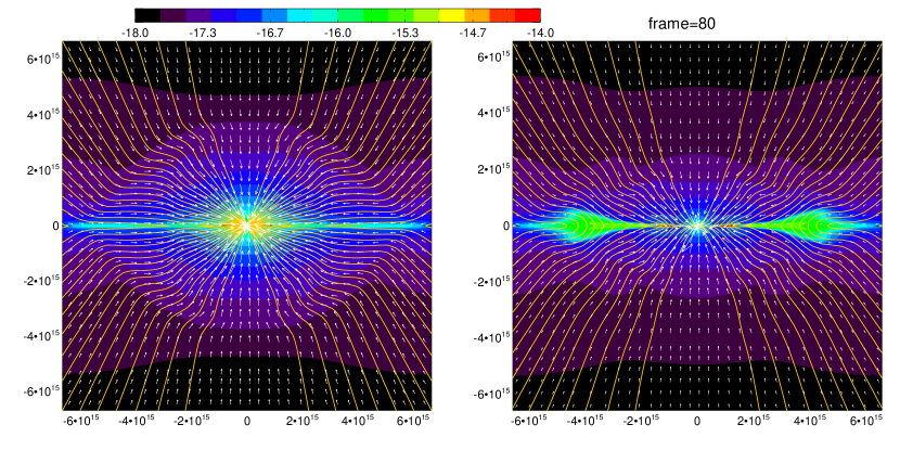
Figure 6: Snapshots of two 2D (axisymmetric) simulations with different inner boundary radii ($r_{i}=10^{14}{\rm\,{\rm cm}}$ for the left panel, and $1.5\times 10^{13}{\rm\,{\rm cm}}$ for the right), showing the magnetic field lines (yellow lines), velocity vectors (white arrows) and the logarithm of density (color map) in the meridian plane. Note the severely pinched field lines before (episodic) reconnection in the left panel, and the two high density equatorial “blobs” created by (episodic) reconnection in the right panel. See movies online.

In any case, the reconnected field lines in the 2D simulations are driven outward by magnetic tension force, leaving behind a strongly magnetized, low density region. This two-step flux redistribution — field line reconnection near the inner boundary followed by outward field advection — is likely operating in our 3D simulations as well. A difference is that, in 3D, mass accretion can continuously drag field lines across the inner boundary along some (azimuthal) directions, with the reconnected field lines escaping outward along other directions. This more continuous reconnection makes individual events less powerful, and thus harder to identify (Zhao et al. 2011; Krasnopolsky et al. 2012), especially in the presence of a turbulence. In the non-turbulent (Model A), and weakly turbulent (Model B and C) cases, the redistributed magnetic flux remains trapped close to the central object, forming a strongly magnetized, low-density region — the DEMS — that is known to be a formidable obstacle to disk formation (Zhao et al. 2011; Krasnopolsky et al. 2012; see Fig. 7). In these cases, the decoupling-triggered reconnection has greatly weakened the central split magnetic monopole, which lies at the heart of the magnetic braking catastrophe in ideal MHD (Galli et al. 2006). However, it created another, perhaps even more severe, problem — the DEMS — which has to be overcome in order for rotationally supported disks to form.

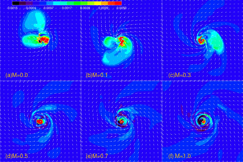
Figure 7: Same as in Fig. 2, except for the color map, which displays the vertical magnetic field strength $B_{z}$ (in units of Gauss) on the equatorial plane. Note the strong anti-correlation between the strongly magnetized region (DEMS, in Models A–C) and rotationally supported disk (in Models D–F). The weakening of DEMS appears to be a prerequisite for disk formation.

3.3 Obstacle to Disk Formation: DEMS

In order for RSDs to form, both the central split magnetic monopole and the DEMS must be weakened. Fig. 5 shows that the amount of magnetic flux $\Phi_{r}$ threading the inner boundary is about the same for the non-turbulent (Model A) and sonic turbulence (Model F) cases, indicating that the weakening of the split magnetic monopole is not controlled by turbulence. As discussed above, it is most likely caused by the decoupling-triggered reconnection observed in the 2D axisymmetric case. The magnetic flux $\Phi_{r}$ is somewhat lower in the turbulent case between $\sim 10^{15}{\rm\,{\rm cm}}$ and $\sim 10^{16}{\rm\,{\rm cm}}$ (see the dashed line in Fig. 5). This could be due to additional, turbulence-enhanced, magnetic reconnection during the core collapse, as advocated by Santos-Lima et al. (2012, see also Santos-Lima et al. 2013 and Joos et al. 2013). Alternatively, it could be related to how the field lines reconnected near the inner boundary escape to large distances, as discussed below in § 4.2. In any case, the difference in $\Phi_{r}$ between these models with and without turbulence is relatively moderate.

A more striking difference lies in the DEMS. Fig. 7, which plots the vertical field strength $B_{z}$ on the equatorial plane, shows that the strongly magnetized DEMS dominates the circumstellar region on the disk-forming, $10^{2}{\rm\,{\rm AU}}$ scale for the non-turbulent and weakly turbulent cases (Models A–C). It becomes much less prominent for the stronger turbulence cases (Models D–F). The turbulence has clearly reduced $B_{z}$ on the equatorial plane (and thus the magnetic flux threading vertically through the plane) near the central object. This reduction may hold the key to understanding the turbulence-enabled disk formation observed in Fig. 2, given the strong anti-correlation between the highly magnetized DEMS and the rotationally supported disk. To quantify the $B_{z}$ reduction, we focus on the net magnetic flux $\Phi_{z}$ that passes vertically through the equatorial plane inside a circle of cylindrical radius $\varpi$:

$$\Phi_{z}(\varpi)=\Phi_{i}+\int_{0}^{2\pi}\int_{\varpi_{i}}^{\varpi}B_{z}(\varpi,\theta=\pi/2,\phi)\varpi\ d\varpi\ d\phi\ ,$$ (5)

where $\Phi_{i}$ is the contribution from the upper hemisphere of the inner (spherical) boundary and $\varpi_{i}=10^{14}{\rm\,{\rm cm}}$.

In Fig. 8, we plot the time evolution of the vertical magnetic flux $\Phi_{z}$ inside a circle of cylindrical radius $\varpi\approx 10^{16}{\rm\,{\rm cm}}$ (left panel) and $3\times 10^{15}{\rm\,{\rm cm}}$ (right panel) for Models A–F. For the larger circle, $\Phi_{z}$ increases more or less monotonically with time in the absence of any turbulence ($M=0$, the upper solid line in the figure). This is to be expected, since more and more field lines are dragged across the circle as the equatorial material collapses. The pause around $t_{k}\sim 5\times 10^{11}{\rm\,{\rm s}}$ is caused by the outer edge of the dense, equatorial pseudodisk (Galli & Shu 1993; see Fig. 14 below for an example) expanding across the circle under consideration; the pseudodisk expansion temporarily lowers the flux $\Phi_{z}$. A similar (although weaker) kink is also visible for the smaller, $\varpi\approx 3\times 10^{15}{\rm\,{\rm cm}}$, circle (see the right panel of Fig. 8). It occurs at an earlier time $t_{k}\sim 10^{11}{\rm\,{\rm s}}$, which is expected since the outer edge of the pseudodisk crosses this smaller circle sooner. The most striking feature for the non-turbulent case is that the magnetic flux inside the smaller circle levels off after $t\sim 5\times 10^{11}{\rm\,{\rm s}}$, and becomes oscillatory. The oscillation is caused by the highly magnetized, low-density structure (DEMS, see Figs. 2 and 7) expanding beyond the circle, advecting back out the magnetic flux dragged across the circle by the collapsing flow in a highly time variable manner.

Figure 8: Time evolution of the magnetic flux $\Phi_{z}$ passing vertically through a circle on the equatorial plane with cylindrical radius $\varpi=1.055\times 10^{16}{\rm\,{\rm cm}}$ (left panel) and $3.055\times 10^{15}{\rm\,{\rm cm}}$ (right panel) for Model A ($M=0$, upper thin solid line), B (dashed), C (dash-dotted), D (long dashed), E (dotted) and F ($M=1$, lower thick solid line). The trend is clear that a stronger turbulence leads to a lower magnetic flux at late times.

In the presence of a turbulence, the time evolution of the magnetic flux $\Phi_{z}$ changes significantly. For the larger circle ($\varpi\approx 10^{16}{\rm\,{\rm cm}}$), as the level of turbulence increases, there is a trend for the kink on the $\Phi_{z}(t)$ curve to start earlier, the turnover to last longer, and the increase after the turnover to become slower. The earlier kink occurs because the outer edge of the pseudodisk is distorted by turbulence, causing it to reach the circle earlier. In the strongest turbulence case (Model F with $M=1$), the magnetic flux stays more or less constant after the kink, at a value well below that of the non-turbulent case at the end of the simulation (by a factor of $\sim 2.4$). Unlike the non-turbulent case discussed in the last paragraph, this leveling off cannot be due to magnetic flux redistribution through the expansion of DEMS, which is apparently absent in Model F (see Fig. 7). For this model, the magnetic flux levels off after the kink for the smaller ($\varpi\approx 3\times 10^{15}{\rm\,{\rm cm}}$) circle as well, at a value lower than that of the non-turbulent case by an even larger factor ($\sim 5$). The leveling off in the increase of magnetic flux is a key to understanding the weakening of the DEMS by turbulence and the appearance of the RSD. Since it starts around the kink when the (perturbed) pseudodisk expands across a circle, it is likely related to the structure of the pseudodisk, a possibility that we will explore next.

3.4 Turbulence-Warped Pseudodisk

In the absence of any turbulence, protostellar accretion in a dynamically significant magnetic field is known to be controlled to a large extent by the pseudodisk (Galli & Shu 1993). To highlight the morphology of the pseudodisk and how it is perturbed by turbulence, we plot in Fig. 9 the density distribution on the surface of a sphere at a representative radius of $r=4.756\times 10^{15}{\rm\,{\rm cm}}$ for Models A–F. It is evident that the mass in the non-turbulent case is highly concentrated near the equatorial plane ($\theta=\pi/2$), in the pseudodisk. The mass concentration is due to matter settling gravitationally along field lines toward the equatorial plane, amplified by the compression by a severely pinched magnetic field (for a pictorial view of the pseudodisk and associated magnetic field in the non-turbulent case, see Fig. 14 below). This pseudodisk is dynamically important because it is where the majority of the core mass accretion occurs. For example, in the non-turbulent case (Model A), if we somewhat arbitrarily assign the region denser than $10^{-17}{\rm\,{{\rm g}{\rm\,{\rm cm}}^{-3}}}$ (bounded by the black solid lines in the figure) to the pseudodisk, then $85\%$ of the mass accretion at the radius shown in Fig. 9 occurs through the pseudodisk, even though it covers only $2.7\%$ of the surface area of the sphere. The concentration of mass accretion in the pseudodisk in the non-turbulent case is an unavoidable consequence of the interplay between the gravity and a dynamically significant, ordered, magnetic field, whose opposition to the gravity is highly anisotropic (Galli & Shu 1993; Allen et al. 2003).

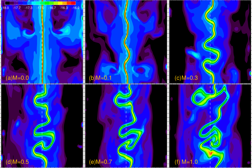
Figure 9: Density distribution on a sphere of representative radius $r=4.756\times 10^{15}{\rm\,{\rm cm}}$ (or about $318{\rm\,{\rm AU}}$) at time $t=5\times 10^{11}{\rm\,{\rm s}}$ for Models A–F. The horizontal axis is the polar angle $\theta$ from $0$ to $\pi$, and vertical axis the azimuthal angle $\phi$ from $0$ to $2\pi$. The equator plane at $\theta=\pi/2$ is marked by a dashed line. The dense, equatorial, pseudodisk in the non-turbulent model becomes increasingly distorted as the level of turbulence increases. The color map shows the logarithm of the density, added to a floor value of $10^{-18}{\rm\,{{\rm g}{\rm\,{\rm cm}}^{-3}}}$. The black solid lines are constant density contours at $10^{-17}{\rm\,{{\rm g}{\rm\,{\rm cm}}^{-3}}}$ used to highlight the pseudodisk.

The presence of a moderate level of turbulence does not change the above picture fundamentally. For example, the $M=0.1$ turbulence in Model B warps the nearly flat pseudodisk in the non-turbulent case only slightly, as seen in panel (b) of Fig. 9. As the level of turbulence increases, the amplitude of pseudodisk warping grows. Nevertheless, the pseudodisk retains its basic integrity even in the strongest turbulence case of $M=1$ (Model F); it is severely distorted, with some portions folding onto themselves (see panel f of the figure), but not completely destroyed.

The turbulence-induced distortion of the pseudodisk can be viewed more vividly in Fig. 10, where we plot two isodensity surfaces at $\rho=10^{-17}$ and $10^{-16}{\rm\,{{\rm g}{\rm\,{\rm cm}}^{-3}}}$ in 3D for the $M=0.3$ and $1$ cases. At the time shown, the corrugation induced by the subsonic, $M=0.3$ turbulence remains relatively moderate. When the turbulent Mach number increases to 1, the pseudodisk, as traced by the red isodensity surfaces, becomes more severely warped and partially folded onto itself, but remains relatively thin. In our simulations, the chaotic turbulent motion is dominated by the fast, ordered, supersonic gravitational collapse in the region where the pseudodisk is formed. This, we believe, is the reason why the pseudodisk is perturbed, rather than completely destroyed, by a subsonic or transonic turbulence. In § 4.2, we will present general arguments for the pseudodisk as a generic feature of magnetized core collapse.

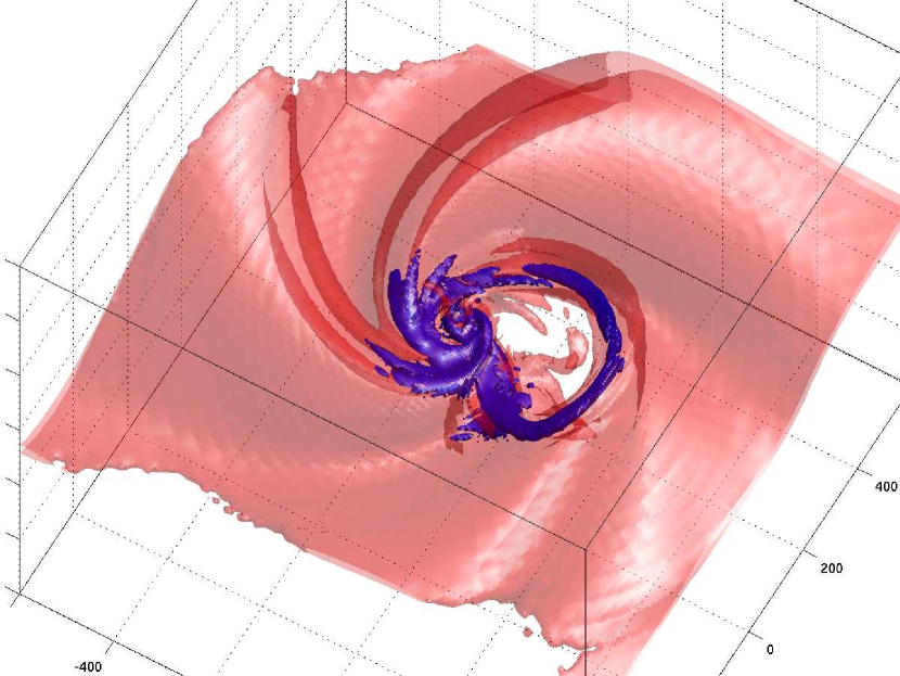
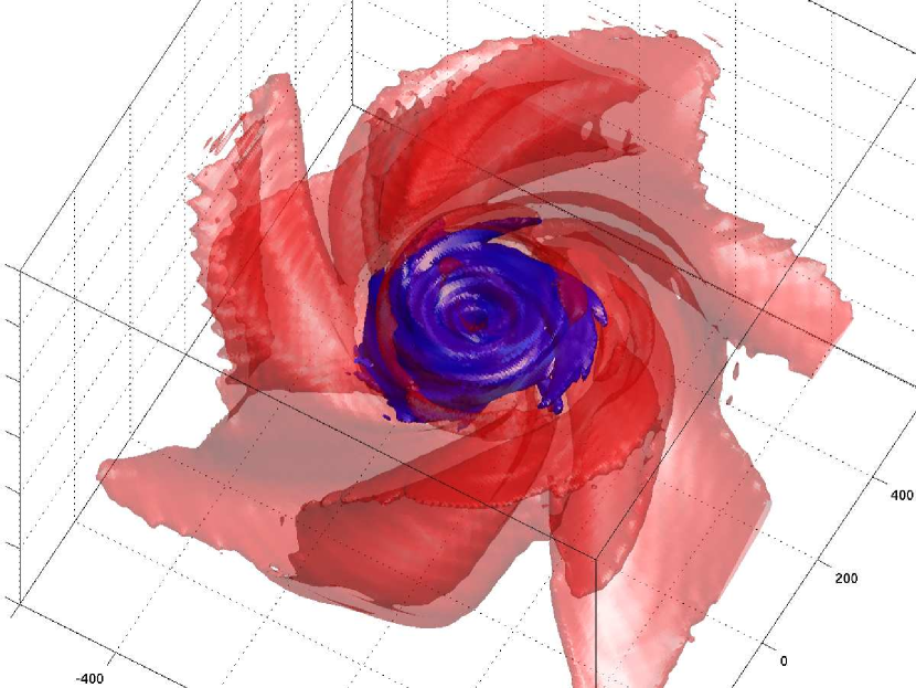
Figure 10: 3D structure of the warped pseudodisk. Plotted are isodensity surfaces at $\rho=10^{-17}$ (red surfaces) and $10^{-16}{\rm\,{{\rm g}{\rm\,{\rm cm}}^{-3}}}$ (blue) for the $M=0.3$ (Model C, left panel) and $1$ (Model F, right panel) case at time $t=8\times 10^{11}{\rm\,{\rm s}}$ (same as in Figs. 2 and 7). Note the corrugation of the pseudodisk (as traced by the red surfaces) induced by turbulence. The blue region roughly corresponds to the rotationally supported disk in the right panel (Model F). The low-density “hole” in the left panel (Model C) corresponds to the strongly magnetized DEMS shown in the upper right panel of Fig. 7. The box size is $1200{\rm\,{\rm AU}}$ on each side.

The warped pseudodisk plays the same fundamental role in the turbulent cases as the flat pseudodisk in the non-turbulent case: it is the main conduit for core mass accretion. For example, on the spherical surface shown in Fig. 9, the warped pseudodisk (bounded by the black density contours) is responsible for $72\%$, $69\%$, $74\%$, $64\%$, and $68\%$ of the mass flux for the $M=0.1$, $0.3$, $0.5$, $0.7$, and $1$ case, respectively, even though it covers only $3.3\%$, $5.9\%$, $7.1\%$, $8.2\%$, and $12.2\%$ of the surface area. Since the collapsing pseudodisk is mainly responsible for the mass accretion that drags the field lines into the circumstellar region close to the central object, it should not be too surprising that its distortion by turbulence affects the magnetic flux accumulation there, as we show next.

3.5 Pseudodisk Warping and Magnetic Flux Reduction

As discussed in § 3.2 and illustrated in Fig. 8, turbulence tends to lower the magnetic flux threading the equatorial plane at small radii at late times. To understand this trend quantitatively, we note that the evolution of the magnetic flux $\Phi_{z}$ enclosed within a circle of fixed cylindrical radius $\varpi$ on the equatorial plane is governed by the induction equation, which can be cast into the following form using the Stokes theorem

$${\partial\Phi_{z}\over\partial t}=\int_{0}^{2\pi}E_{\phi}\ \varpi\ d\phi=-\int_{0}^{2\pi}v_{\varpi}B_{z}\ \varpi\ d\phi+\int_{0}^{2\pi}v_{z}B_{\varpi}\ \varpi\ d\phi,$$ (6)

in a cylindrical coordinate system $(\varpi,\phi,z)$. The quantity $E_{\phi}=-v_{\varpi}B_{z}+v_{z}B_{\varpi}$ is the azimuthal component of the electromotive force (EMF) on the circle. On the equatorial plane, the relevant components of the velocity and magnetic field in cylindrical and spherical coordinates are related through $v_{\varpi}=v_{r}$, $B_{\varpi}=B_{r}$, $v_{z}=-v_{\theta}$ and $B_{z}=-B_{\theta}$. The first term on the right hand side of the above equation, $T_{\phi,r}=\int_{0}^{2\pi}v_{r}B_{\theta}\ \varpi\ d\phi$, has an obvious interpretation: it is simply the rate of flux advection by radial infall, which tends to increase the flux $\Phi_{z}$ (and thus be positive) by dragging vertical field lines into the circle. The meaning of the second term $T_{\phi,z}=-\int_{0}^{2\pi}v_{\theta}B_{r}\ \varpi\ d\phi$ is less obvious; it is the rate of flux advection by vertical motions (along the $z$-axis, perpendicular to the equatorial plane) that can move radial field lines across the circle on the equatorial plane.

It is easy to compute $T_{\phi,r}$ and $T_{\phi,z}$ for any radius $\varpi$. As an example, we plot in Fig. 11 their values at $\varpi=1.055\times 10^{16}{\rm\,{\rm cm}}$ as a function of time for different models. At early times, the radial flux advection term $T_{\phi,r}$ dominates the vertical flux advection term $T_{\phi,z}$ for all cases. This is to be expected, because the field lines near the equator remain predominantly vertical outside the pseudodisk (see Figs. 12 and 14 below). After the outer edge of the pseudodisk passes through the circle, the magnetic fluxes in the non-turbulent and weakly turbulent cases start to increase again (see the left panel of Fig. 8). This is because the vertical flux advection that tends to move field lines out of the circle (i.e., $T_{\phi,z}$ tends to be negative), starts to drop below the radial flux advection that tends to move field lines into the circle. An exception is the strongest turbulence case of $M=1$, where the vertical and radial advection terms stay comparable, so that the magnetic flux changes relatively little at late times. Fig. 11 shows clearly that the more efficient outward transport of magnetic flux by vertical motions is the main reason for the slower flux increase for a stronger turbulence. In order for the outward flux transport to be efficient, both $v_{\theta}$ and $B_{r}$ need to have a relatively large value, which can be achieved when a pseudodisk with a highly pinched magnetic field (i.e., an appreciable $B_{r}$) is strongly perturbed vertically (i.e., an appreciable $v_{\theta}$), by turbulence or some other means.

Figure 11: The rates of magnetic flux change, $T_{\phi,r}$ and $T_{\phi,z}$ (in cgs Gaussian units), across a circle of radius $\varpi=1.055\times 10^{16}{\rm\,{\rm cm}}$ on the equatorial plane due to, respectively, radial advection of vertical field $B_{\theta}$ by infall (with $v_{r}$; upper curves) and vertical advection of radial field $B_{r}$ by vertical motions (with $v_{\theta}$; lower curves), for Model A ($M=0$, thin solid line), B (dashed), C (dash-dotted), D (long dashed), E (dotted) and F ($M=1$, thick solid line). Note that turbulence increases the rate of outward (or negative) magnetic flux advection by vertical motions.

To illustrate how a strongly perturbed pseudodisk can slow down the magnetic flux accumulation inside a circle more pictorially, we plot in Fig. 12 the density distribution and magnetic field (unit) vectors on a representative meridian plane for the $M=1$ case. Note that the turbulence-driven warping moves the pseudodisk above (see the loop to the right of the disk) and below (see the loop to the left) the equatorial plane. The above-the-equatorial-plane loop (on the right side) delivers a substantial amount of matter through the upper hemisphere (marked by the dashed line in the figure) but little net magnetic flux; the sharp kink of field lines across the loop allows most of the field lines dragged into the hemisphere by the accreting loop to return through the same hemisphere, without crossing or touching the circle on the equatorial plane (marked by two red crosses on the figure); a similar case can be made for the lower hemisphere. This is in contrast with the mass accretion through the unperturbed equatorial pseudodisk, which must be accompanied by a flux increase (in the ideal MHD limit). Since the net magnetic flux going through the upper (or lower) hemisphere is the same as that through the equatorial plane that bisects the sphere, the pseudodisk warping provides a natural explanation for the lower magnetic flux accumulated close to the central object on the equatorial plane (and thus a weaker DEMS) that we found for a stronger turbulence.

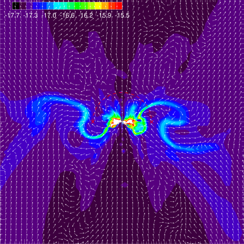
Figure 12: Density map and magnetic field unit vectors of the $M=1$ model on a meridian plane at a representative time $t=8\times 10^{11}{\rm\,{\rm s}}$. It illustrates how an out-of-the-equatorial-plane dense loop (the loop on the right side, part of the warped pseudodisk) can bring matter through the upper hemisphere (dashed line) but little magnetic flux. The two crosses mark where the hemisphere and equatorial plane intersect. The length of the box is $5\times 10^{16}{\rm\,{\rm cm}}$ on each side. The colorbar is as in Fig. 2.

3.6 Torque Analysis

Whether a rotationally supported disk can form or not depends on the amount of angular momentum that is initially available on the core scale and that is removed by magnetic torque and outflow as the rotating core material collapses toward the central object. We follow Li et al. (2013) in evaluating the $z$-components of the dominant magnetic torque due to the magnetic tension force (as opposed to the magnetic pressure gradient) and the advective torque:

$$N_{t,z}=\frac{1}{4\pi}\int\varpi B_{\phi}B_{r}\ dS,$$ (7)

and

$$N_{a,z}=-\int\rho\varpi v_{\phi}v_{r}\ dS,$$ (8)

where $\varpi$ is the cylindrical radius, and the integration is over the surface $S$ of a sphere of radius $r$. They measure, respectively, the rate of angular momentum change in the volume enclosed by the surface $S$ due to magnetic braking and matter crossing the surface $S$. The advective torque consists of two parts: the rates of angular momentum advected into and out of the sphere by infall and outflow respectively:

$$N_{a,z}^{\rm{in}}=-\int\rho\varpi v_{\phi}v_{r}(<0)\ dS,$$ (9)

and

$$N_{a,z}^{\rm{out}}=-\int\rho\varpi v_{\phi}v_{r}(>0)\ dS.$$ (10)

We have examined the radial distributions of the magnetic and advective torques for Models A–F and at different times. The basic features of the distributions are well illustrated in the examples shown in Fig. 13. To avoid crowding, we have shown only two extreme cases (with $M=0$ and $1$). The right panel of the figure, which displays the net torque, shows that, in the non-turbulent case, the magnetic torque is large enough to remove essentially all of the angular momentum advected inward at all radii inside $\sim 10^{16}{\rm\,{\rm cm}}$; indeed, it is so strong as to cause a net decrease in angular momentum between $\sim 3\times 10^{15}$ and $\sim 10^{16}{\rm\,{\rm cm}}$. This latter feature is in striking contrast with the $M=1$ case, where the magnetic torque is not large enough to remove all of the angular momentum brought in by flows. The imbalance leaves a substantial net (positive) torque between $\sim 3\times 10^{15}$ and $\sim 10^{16}{\rm\,{\rm cm}}$, which increases the angular momentum of the material in this region, enabling a rotationally supported disk to form in this case. Since the difference between the two cases appears most prominent near $r\sim 10^{16}{\rm\,{\rm cm}}$, we will first focus on this region in our effort to understand why the magnetic braking is so efficient in the non-turbulent case and why the efficiency is significantly decreased by the $M=1$ turbulence.

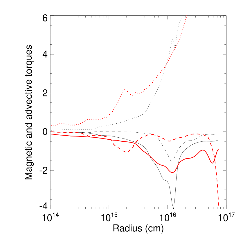
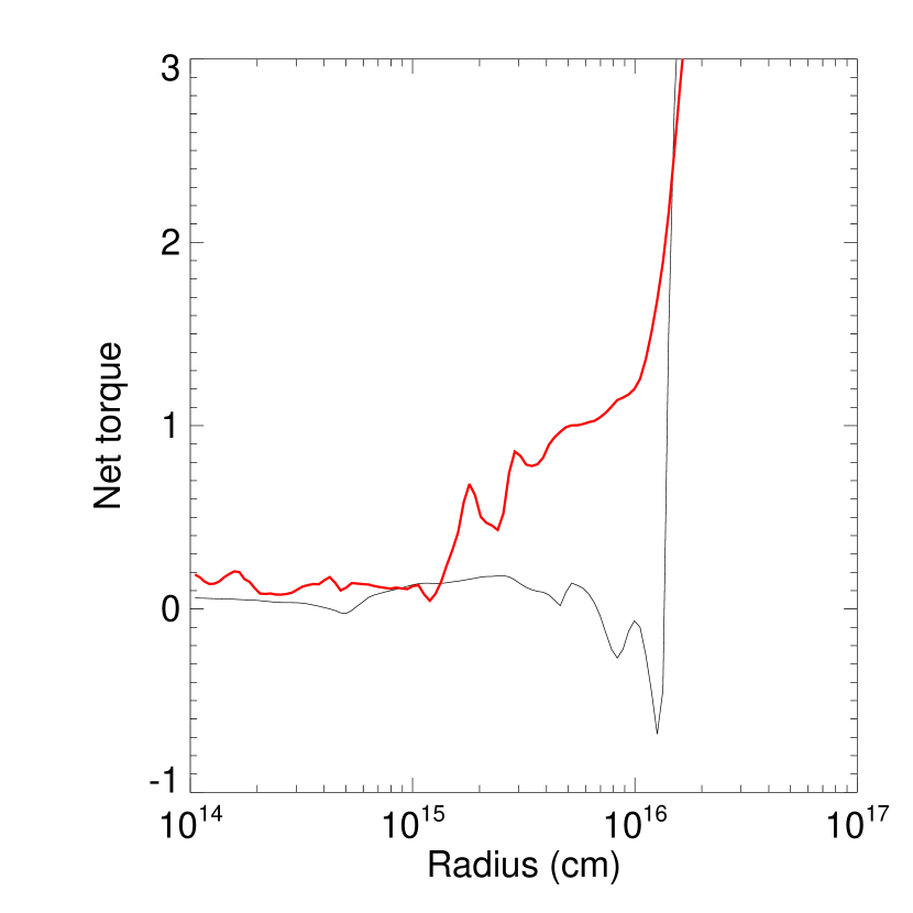
Figure 13: Left panel: Magnetic torques (solid lines, $N_{t,z}$) and advective torques ($N_{a,z}$) by infall ($N_{a,z}^{\rm{in}}$, dotted) and outflow ($N_{a,z}^{\rm{out}}$, dashed) acting on spheres of different radii for models with $M=0$ (thin black lines) and 1 (thick red lines), at a representative time $t=7\times 10^{11}{\rm\,{\rm s}}$ for Model F. Right panel: The net torque ($N_{t,z}+N_{a,z}$) for the same two cases. The torques are in units of $10^{40}{\rm\,{\rm dyn}}{\rm\,{\rm cm}}$.

We first concentrate on the non-turbulent case. It turns out that the $r\sim 10^{16}{\rm\,{\rm cm}}$ region is rather special; it includes the outer part of the pseudodisk. This is illustrated in Fig. 14, where we display the density map on a meridian plane (which shows the pseudodisk clearly) and unit vectors for the magnetic field at the same representative time as in Fig. 13. The two crosses mark the locations where the magnetic torque peaks (at $r\approx 1.3\times 10^{16}{\rm\,{\rm cm}}$). It is clear that, as matter enters the equatorial pseudodisk, it drags the field lines into a highly pinched configuration (note the reversal of the radial field above and below the pseudodisk). Associated with the pinch is a large magnetic tension force in the radial direction, which acts against the gravity and retards the collapse significantly. The retardation can be seen in Fig. 15, which shows that the azimuthally averaged infall speed on the equator is suddenly reduced by about a factor of two right outside $r\sim 10^{16}{\rm\,{\rm cm}}$, precisely where the rate of magnetic braking peaks. This region of sharp deceleration of the magnetized collapsing flow is termed the “magnetic barrier” by Mellon & Li (2008, see their Fig. 4); this barrier is analogous to the well-known “centrifugal barrier” where the infall is quickly slowed down by rotation. The slow-down allows both matter and magnetic field lines to pile up, signaling the formation of a dense, strongly magnetized pseudodisk. The pileup of field lines can be seen in the right panel of Fig. 15, which shows that the vertical component of the magnetic field on the equator, $B_{z}$, increases sharply by a factor of $\sim 3$ at the magnetic barrier. The increased field strength, coupled with severe field pinching (which increases the lever arm for magnetic braking, see Fig. 14), is the reason behind the efficient braking at the magnetic barrier in the non-turbulent case.

Figure 14: Density map and magnetic field unit vectors on a meridian plane for the non-turbulent case at a representative time $t=7\times 10^{11}{\rm\,{\rm s}}$, showing a prominent equatorial pseudodisk and severe field pinching across it (an axial dense spot has been erased for better clarity of the equatorial region). The two crosses mark the locations where the magnetic torque shown in Fig. 13 peaks. The colorbar is as in Fig. 2. The length of the box is $5\times 10^{16}{\rm\,{\rm cm}}$ on each side.

Figure 15: Distributions of the azimuthally averaged infall speed ($v_{r}$, left panel) and vertical field strength ($B_{z}$, right) on the equatorial plane for the non-turbulent case shown in Fig. 14. Note the sharp slow-down of infall and increase in field strength just outside $r=10^{16}{\rm\,{\rm cm}}$, precisely where the magnetic torque peaks.

In the presence of a sonic turbulence ($M=1$), the peak rate of angular momentum removal by magnetic torque is substantially reduced (by a factor of $\sim 2$, see Fig. 13). Our interpretation is that the reduction is due to the distortion of the highly coherent magnetic barrier of the $M=0$ case by turbulence. Fig. 12 shows that the transition from the infall envelope to the pseudodisk is less coherent and more gradual in the $M=1$ case compared to the $M=0$ case (Fig. 14). As a result, the rotation is braked more gently as the matter enters the (highly warped) pseudodisk. The weaker braking at the outer part of the pseudodisk leaves the material inside the pseudodisk with more angular momentum, making it more likely to form a rotationally supported disk.

Another difference between the $M=0$ and $1$ case lies in the outflow. In the non-turbulent case, the outflow is driven mostly by the equatorial (rotating) pseudodisk, which winds up the field lines, building up a magnetic pressure near the equatorial plane that is released by (bipolar) expansion away from the plane. On the scale of the pseudodisk ($\sim 10^{16}{\rm\,{\rm cm}}$) that is crucial for disk formation, the outflow removes angular momentum at a rate that is a substantial fraction (typically $\sim 1/3$ to $1/2$) of that by magnetic torque (see the left panel of Fig. 13 for an example). This is in contrast with the $M=1$ case, where the angular momentum removal by outflow is much less efficient on the same scale (see Fig. 13). The lower efficiency is most likely caused by the severe warping of the pseudodisk, which weakens the ability of the rotating material in the warped pseudodisk to generate a coherent toroidal field for outflow driving (a similar point was also made in Seifried et al. 2012, 2013). Furthermore, the outflow, if driven at all, will consist of strands coming from different parts of the warped pseudodisk, which may have different orientations; strands moving in different directions may lead to cancellation that weakens the net efficiency of the outward angular momentum transport by the outflow. We should note that, at smaller radii (on the $\sim 10^{15}{\rm\,{\rm cm}}$, rotationally supported disk-scale), the outflow in the $M=1$ case removes angular momentum more efficiently than that in the $M=0$ case. This outflow is driven by the RSD, and is thus a consequence of, rather than the cause for, the disk formation. Nevertheless, it removes angular momentum from the RSD, and could threaten its survival; it may have contributed to the destruction of the transient disks in the $M=0.5$ and $0.7$ cases (Models D and E in Table 1).

3.7 Varying Initial Turbulent Velocity Field

We have carried out several shorter duration simulations with different turbulent velocity fields to explore their effects on disk formation. Two examples are shown in Fig. 16. They are identical to Model F (with $M=1$ and an exponent for the turbulent velocity spectrum $p=1$), except for $p=0.5$ (Model U) or $2.0$ (Model V). In both cases, a rotationally supported disk is formed at the time shown ($t=6\times 10^{11}{\rm\,{\rm s}}$), just as in Model F. The disk is somewhat larger and better developed in Model U than in Model V, indicating that the shallower turbulent velocity spectrum (with more power at shorter wavelength) is more conducive to disk formation. However, we refrain from drawing more quantitative conclusions because the turbulent velocity fields are distorted by our non-uniform grid due to the undersampling of the high-frequency part of the velocity spectrum at large radii, where the spatial resolution is relatively coarse.

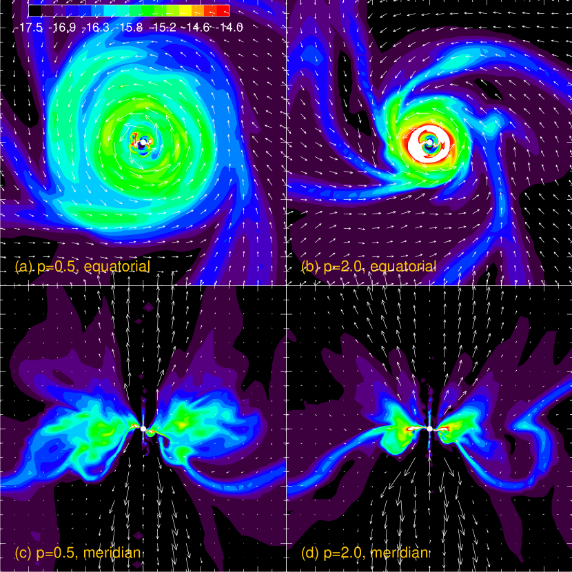
Figure 16: Density map and velocity field for Model U ($p=0.5$, left panels) and V ($p=2.0$, right panels) on the equatorial (top panels) and a meridian (bottom panels) plane at time $t=6\times 10^{11}{\rm\,{\rm s}}$. A well developed disk is apparent in both cases. The colorbar is as in Fig. 2. The length of the box is $10^{16}{\rm\,{\rm cm}}$ on each side.

4 Discussion

4.1 Unification of Turbulence- and Misalignment-Enabled Disk Formation

The warping of pseudodisk out of the disk-forming equatorial plane by turbulence plays a central role in our interpretation of the robust disk formation observed in our simulations. Pseudodisk warping was also the key ingredient of another proven mechanism for disk formation: misalignment between the magnetic field and rotation axis (Hennebelle & Ciardi 2009; Joos et al. 2012; Krumholz et al. 2013; Li et al. 2013). Since our problem setup is somewhat different from those of previous studies (they included self-gravity that is ignored here, see § 2), we have rerun the non-turbulent case (Model A) but with the magnetic field perpendicular to the rotation axis (Model P in Table 1). A robust rotationally supported disk is easily formed in this case, as shown in the left panel of Fig. 17. As in the case with self-gravity, there are two prominent spiral arms in the equatorial density map of Fig. 17, which are part of a pseudodisk that lies almost perpendicular to the equatorial plane initially and is wrapped by rotation into a snail shell-like structure in 3D (see Fig. 2 of Li et al. 2013).

Although the warping of the pseudodisk in Model P is more extreme and less chaotic than that induced by the sonic turbulence ($M=1$) in Models F, U and V, the underlying physical reason for disk formation and survival appears broadly similar. Specifically, the large field-rotation misalignment ensures that the bulk of the pseudodisk material stays out of the equatorial plane, which alleviates the problem of magnetic flux ($\Phi_{z}$) accumulation on the equatorial plane. This in turn eliminates the highly magnetized DEMS that is detrimental to disk formation (Zhao et al. 2011; Krasnopolsky et al. 2012), as shown in the right panel of Fig. 17. In addition, the misalignment decreases the rate of angular momentum removal from the pseudodisk by outflow (Ciardi & Hennebelle 2010; Li et al. 2013) and weakens the braking near the magnetic barrier, both of which leave more angular momentum in the accretion flow to form RSDs. The turbulence- and misalignment-enabled disk formation are thus unified, in that both cause the pseudodisk to warp strongly out of the equatorial plane (defined by rotation), which is conducive to disk formation.

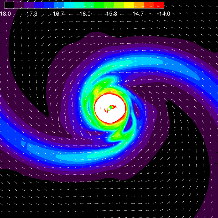
Figure 17: Distribution of the logarithm of density (in ${{\rm g}{\rm\,{\rm cm}}^{-3}}$) and velocity field (left panel) and the vertical component of the magnetic field $B_{z}$ and velocity field (right panel) on the equatorial plane at a representative time $t=8\times 10^{11}{\rm\,{\rm s}}$ for Model P where the magnetic field is perpendicular to the rotation axis. The two prominent spirals in the left panel are part of the strongly warped pseudodisk that feeds the central rotationally supported disk. The central, white part has a density above the maximum value for the color plot, which is set to a relatively low value in order to highlight the spirals. The right panel shows that the strongly magnetized DEMS that prevented disk formation in the aligned, non-turbulent and weakly turbulent cases (see Fig. 7) disappears almost completely, strengthening the case for the elimination of DEMS as a prerequisite for disk formation. The length of the box is $2\times 10^{16}{\rm\,{\rm cm}}$ on each side for both panels.

4.2 Origin of Rotationally Supported Disks

The pseudodisk that plays a central role in our scenario of RSD formation is a generic feature of the protostellar collapse channeled by a large-scale, dynamically significant magnetic field. This is because the material distributed along any given field line cannot all collapse toward the center at the same rate; some part is bound to collapse in a runaway fashion, as illustrated in the upper panel of Fig. 18. If a piece of matter on a field line is initially closer to the central object than the rest of the material along the same field line, it would experience a stronger gravitational acceleration, which would move it closer to the center, which would in turn increase its gravitational acceleration further. This differential collapse of matter along a field line drags the field line into a highly pinched configuration, which would not only allow matter to slide along the field line to the cusp but also compress the material collected there into a flattened structure — the pseudodisk (Galli & Shu 1993; Allen et al. 2003). It is the conduit for most of the core mass accretion with or without a turbulence, as discussed in § 3.4 and illustrated in Fig. 9. As such, it is largely responsible for concentrating the magnetic flux at small radii that creates the difficulty for RSD formation in the first place. Fortunately, it also holds the key to overcoming the difficulty.

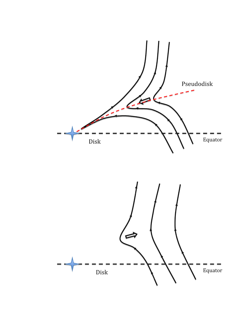
Figure 18: Cartoon illustrating pseudodisk formation and magnetic flux loss from the equatorial, disk-forming region close to the central object. Top panel: localized runaway gravitational collapse drags the field lines into a highly pinched configuration, which enables matter to slide along field lines and collect at the apex to form a dense pseudodisk, which is further compressed magnetically. The out-of-the-equatorial-plane warping enables the pseudodisk to deliver mass close to the center object without increasing the magnetic flux in the circumstellar disk-forming region on the equatorial plane. Bottom panel: the highly pinched field lines reconnect near the central object, triggered by magnetic decoupling near the central object or some other means. The reconnected field lines are driven outward by the magnetic tension, escaping to large distances.

The key is the sharp field reversal across the pseudodisk (see Fig. 18). The highly pinched field lines are prone to magnetic reconnection, numerical or otherwise. There is little doubt that reconnection has occurred in all magnetized disk formation simulations to date that include turbulence (Santos-Lima et al. 2012, 2013; Seifried et al. 2012, 2013; Joos et al. 2013; Myers et al. 2013). It is needed to explain the loss of magnetic flux near the central protostar relative to that expected under flux-freezing found in these simulations. Santos-Lima et al. (2012) was the first to study the flux loss, and attributed it to the turbulence-induced magnetic reconnection (Lazarian & Vishniac 1999; Kowal et al. 2009), which in their scenario is the key to disk formation (see also Santos-Lima et al. 2013). Joos et al. (2013) found that the amount of flux loss increases with the level of turbulence, as one would expect if the flux loss is induced by turbulent reconnection. This is, however, not definitive proof of Santos-Lima et al.’s scenario, because the turbulence-induced reconnection events remain to be identified in the simulations.

We propose an alternative scenario for the reconnection that is required to explain the flux reduction observed in simulations, including our own: the magnetic decoupling-triggered reconnection of sharply pinched field lines. This alternative is motivated by the fact that gravitational collapse can naturally produce, by itself, sharply pinched field lines close to the central object that are prone to reconnection and that flux reduction is observed even in non-turbulent simulations, such as our Models A and P (see also Zhao et al. 2011 and Krasnopolsky et al. 2012), which indicates that efficient reconnection can be achieved without any turbulence. This type of reconnection was observed directly in 2D (axisymmetric) simulations of Mellon & Li (2008, see also footnote 2, Fig. 6, and auxiliary material online), where oppositely directed field lines above and below the pseudodisk reconnect episodically near the inner boundary, where the matter is decoupled from the field lines as it accretes onto the central object. As discussed in § 3.2, the decoupling is required for solving the “magnetic flux problem” in star formation, and may be achieved physically through non-ideal MHD effects (e.g., Li & McKee 1996; Contopoulos et al. 1998; Kunz & Mouschovias 2010; Machida et al. 2011; Dapp & Basu 2010; Dapp et al. 2012; Tomida et al. 2013). In our scenario, it is responsible for preventing the field lines from piling up near the center to form the strong split magnetic monopole that lies at the heart of the “magnetic braking catastrophe” in ideal MHD (Galli et al. 2006).

The elimination of the split monopole does not guarantee RSD formation, however. In the absence of any turbulence (or field-rotation misalignment), the bulk of core mass accretion is funneled through a dense, coherent, equatorial pseudodisk (see Fig. 14). The accreting material drags the field lines to the inner boundary, where they decouple from the matter. After decoupling, the oppositely directing field lines above and below the equator reconnect, and are driven outward by the magnetic tension force along the equatorial plane. However, their equatorial escape to large distances is blocked by continuous mass infall in the dense, coherent, equatorial pseudodisk. They remain trapped close to the central object, in a highly magnetized circumstellar region — the DEMS. As discussed in § 3.3 and illustrated in Fig. 7, the DEMS must be removed in order for a robust, rotationally supported disk to form (Zhao et al. 2011; Krasnopolsky et al. 2012). This, in our scenario, is where turbulence (and field-rotation misalignment) comes in.

In the presence of a strong turbulence, the pseudodisk can become severely warped out of the equatorial plane and highly variable in time. The beneficial effect of pseudodisk warping to disk formation is illustrated in the top panel of the cartoon in Fig. 18. Mass accretion through the warped pseudodisk will still drag along the (highly pinched) field lines. However, unlike the case of flat equatorial pseudodisk, such field lines do not have to pass through the circumstellar, disk-forming region on the equatorial plane; they can cross the equatorial plane at larger distances. The situation is qualitatively similar in the presence of a large field-rotation misalignment, which warps the plane of pseudodisk away from the plane of disk formation. In both cases, when the highly pinched field lines threading the warped pseudodisk reconnect, they can escape directly to large distances without having to cross the equatorial disk-forming region first (see the lower panel of Fig. 18). As a result, the amount of magnetic flux trapped in the equatorial, disk-forming region is much reduced compared to the non-turbulent, field-rotation aligned case. The reduction greatly weakens the DEMS, making the disk formation possible.

Our proposed scenario of RSD formation in turbulent magnetized dense cores thus involves two conceptually distinct steps: (1) decoupling-triggered reconnection of sharply pinched field lines close to the protostar, which removes the strong split magnetic monopole at the center, the first obstacle to disk formation, and (2) warping of the pseudodisk out of the disk-forming plane, which weakens the DEMS, the second obstacle to disk formation. Compared to Santos-Lima et al.’s scenario of turbulence-induced reconnection, it has the advantage of being capable of explaining the disk formation enabled by both turbulence and field-rotation misalignment. Nevertheless, the two scenarios are not mutually exclusive. Indeed, it is likely that both mechanisms are operating in the current generation of simulations. For example, field-matter decoupling must be present in any magnetized disk formation simulations involving sink particles, including those of Santos-Lima et al. (2012, 2013), because the matter is accreted onto the sink particle but not the magnetic field. On the other hand, turbulence has been shown to enhance the reconnection rate of oppositely directed field lines, both analytically (Lazarian & Vishniac 1999) and numerically (e.g., Kowal et al. 2009), so the turbulence-induced reconnection is likely present in simulations, including our own, although its rate is difficult to quantify. We should stress that, even in Santos-Lima et al.’s scenario, the pseudodisk is expected to play a central role: its sharply pinched field lines make it the most natural location for the turbulence-induced reconnection. Furthermore, the warping of the pseudodisk, a key ingredient of our scenario, can help such reconnected field lines escape to large distances without passing through (and being trapped in) the equatorial, disk-forming region. One complication is that the turbulent motions are expected to be strongly modified, indeed dominated, by supersonic gravitational infall in the pseudodisk region close to the central object. The potential effect of such fast infall on the turbulence-induced magnetic reconnection remains to be quantified. Another complication is that, in ideal MHD simulations, both turbulence-induced and decoupling-triggered reconnections involve numerical diffusion, which depends on numerical resolution. As such, it would be difficult to obtain numerically converged solutions.

4.3 Characteristics of Disks Fed by Warped, Magnetized Pseudodisks

A key finding of our investigation is that the rotationally supported disks formed in turbulent, magnetized cloud cores are fed by highly variable, strongly warped pseudodisks. An interesting characteristic of such disks is their thickness. It is illustrated in the left panel of Fig. 19 for Model F (with a turbulent Mach number $M=1$); the figure is a zoom-in of Fig. 12 (see also the lower panels of Fig. 16 for Models U and V). For comparison, we also plotted side-by-side the disk formed in a model that is neither magnetic nor turbulent, but with other parameters identical to those of Model F (Model H in Table 1). The disk in the magnetized Model F is smaller in radius and thicker (relative to radius) than that in the hydro Model H. The smaller radius is to be expected because of angular momentum removal by magnetic braking and the associated outflow. The larger thickness may be due, at least in part, to the feeding of the disk by a strongly warped pseudodisk from directions that are highly variable and often tilted significantly away from the equatorial plane (see auxiliary material online for a movie of mass accretion in a meridian plane); indeed, the warped pseudodisk often feeds the rotationally support disk from the top and bottom surfaces, rather than the outer edge of the disk. As a result, the disk is dynamically “hotter” (with faster motions) in the poloidal plane than that in the hydro case (compare the disk velocity fields in Fig. 19; see below for another mechanism for puffing up the disk).

Figure 19: Disk comparison. Plotted are the distribution of logarithm of density and velocity field on a representative meridian plane for the magnetized, turbulent case of Model F ($M=1$, left panel) and its non-magnetic and non-turbulent counterpart (Model H, right panel) at the same time ($t=8\times 10^{11}{\rm\,{\rm s}}$). Note that the disk in the former appears thicker and more dynamically active than in the latter. The length of the box is $9\times 10^{15}{\rm\,{\rm cm}}$ (or $600{\rm\,{\rm AU}}$) on each side. The colorbar is as in Fig. 2. An axial dense spot has been erased for better clarity of the equatorial region. The velocity vectors are plotted with the maximum speed capped at $10^{5}{\rm\,{{\rm cm}{\rm\,{\rm s}}^{-1}}}$, also for clarity.

Another characteristic of the disks fed by warped pseudodisks is that they are significantly magnetized. This is because the pseudodisks are necessarily magnetized to a significant level since they are the product of magnetically-channeled gravitational collapse. Significant magnetization is therefore expected for the disks as well. The degree of disk magnetization is shown in Fig. 20, where we plot the time evolution of the ratios of magnetic to thermal and rotational to thermal energies for the disk (defined somewhat crudely as the region denser than $10^{-16}{\rm\,{{\rm g}{\rm\,{\rm cm}}^{-3}}}$, a density corresponding to the blue isodensity surface in Fig. 10) for the sonic turbulence cases (Models F, U and V). It is clear that the magnetic energy dominates the thermal energy, by a factor of a few to several for all three cases. The magnetic energy is less than the rotational energy, however, by about one order of magnitude. The magnetic field is therefore expected to be wrapped by rotation into a predominantly toroidal configuration. This is indeed the case, as illustrated in Fig. 21, where representative magnetic field lines are plotted for the disk of Model F shown in the left panel of Fig. 19. The toroidal field configuration is consistent with the recent dust polarization observations of the young disk in IRAS 16293B (Rao et al. 2014), HL Tau (Stephens et al. 2014) and L1527 (Segura-Cox et al. 2014).

Figure 20: Time evolution of the ratios of the magnetic to thermal (lower thicker lines) and rotational to thermal (upper thinner lines) energies for the disk in Model F ($p=1$, solid lines), U ($p=0.5$, dashed) and V ($p=2.0$, dotted), showing that the disk remains strongly magnetized.

Figure 21: 3D magnetic field structure of the disk shown in the left panel of Fig. 19. Plotted are representative magnetic field lines and isodensity surface at $10^{-16}{\rm\,{{\rm g}{\rm\,{\rm cm}}^{-3}}}$ (blue). The box size is $600\times 300{\rm\,{\rm AU}}$.

The two characteristics of the disks discussed above (large thickness and significant magnetization) may be related. The rather strong toroidal field inside the disk provides an additional support (on top of the thermal pressure) to the gas in the vertical direction, which tends to puff up the disk. Observational evidence for a puffed-up disk may already exist. Tobin et al. (2013) inferred, through detailed modeling of the L^′-band image, that the young disk in L1527 is thicker than those in more evolved sources on the $100{\rm\,{\rm AU}}$ scale; it is about twice the disk scale-height estimated based on the thermal support alone. To puff up a disk by a factor of 2, an additional (non-thermal) energy density of $\sim 3$ times the thermal energy density is needed, since the scale-height is proportional to the square root of the total (thermal and non-thermal) energy density. From Fig. 20, it is clear that the required non-thermal energy is comparable to the magnetic energy in the disk. It is therefore plausible that the puffed-up disk in L1527 is an example of the kind of thick, dynamically active disks fed anisotropically by highly variable, strongly warped, magnetized pseudodisks that we find in our simulations (and possibly in the simulations of Santos-Lima et al. 2012, 2013; Seifried et al. 2012, 2013; Myers et al. 2013 and Joos et al. 2013 as well). High resolution observations of polarized dust emission from the disks of L1527 and other deeply embedded sources using sub/millimeter interferometers (especially ALMA) can help firm up or refute this interpretation. In any case, the disk thickness compared to the thermal scale-height can put an upper limit on the disk toroidal field strength, which is difficult to constrain through other means.

4.4 Implications, Uncertainties and Future Directions

The picture of disk-feeding by a variable, warped magnetized pseudodisk, if true in general, may have strong implications for the chemical connection between the collapsing core and the disk; the connection is an important step toward understanding the chemical heritage of the solar system (e.g., Caselli & Ceccarelli 2012; Hincelin et al. 2013). First, if most of the disk-forming material comes from the magnetically compressed pseudodisk, its density before entering the RSD should be higher than that in the non-magnetic (hydro) case. The higher density could affect the rates of chemical reactions and ice formation (for example, through shorter adsorption timescales, or perhaps three-body reactions if the density is high enough), and thus the gas and ice composition. Second, disk-feeding through a highly variable pseudodisk means that any accretion shock, if exists at all, is strongly time dependent and spatially localized, unlike the simplest hydro case where a well-defined accretion shock encases the whole disk (see, e.g., Yorke et al. 1993, and the right panel of Fig. 19). The shock structure is expected to be further modified by the magnetic field embedded in the pseudodisk. As a result, the disk material may experience a rather different thermal history, which could affect both its gas and ice content (e.g., Visser et al. 2009). Third, if the disk is puffed up and dynamically active in the poloidal plane (see the left panel of Fig. 19), its rates of chemical reactions and vertical mixing would be affected. Furthermore, the long-term evolution of the disk is expected to be strongly modified, perhaps dominated, by the rather strong (toroidal) magnetic field in the disk. A caveat is that the disk magnetic energy may be strongly affected by non-ideal MHD effects, which are expected to be important since the bulk of protostellar disks is lightly ionized (Armitage 2011; Turner et al. 2014). The modifications need to be quantified in the future.

Another caveat is that, in our simulations, we included the gravity from a central object (of $0.5{\rm\,{\rm M_{\odot}}}$) but not the self-gravity of the gas. One consequence of this idealization is that the gravity is stronger at small radii compared to the more self-consistent case with self-gravity before the central object accretes $0.5{\rm\,{\rm M_{\odot}}}$. The stronger gravity is expected to accelerate the material in the pseudodisk to a higher infall speed relative to the more slowly collapsing material at larger distances that is magnetically connected to it. The higher relative speed is expected to stretch the field lines across the pseudodisk into a more severely pinched configuration, which should in turn compress the pseudodisk to a smaller thickness. This has the benefit of bringing the role of pseudodisk on disk formation into a sharper focus, but it may have exaggerated that role somewhat. Nevertheless, the presence of a pseudodisk in self-gravitating magnetized protostellar collapse is well established. The fact that we are able to reproduce the known results that disk formation in non-turbulent cores is suppressed when the magnetic field and rotation axis are aligned (Model A) and enabled when they are orthogonal (Model P) gives us confidence that, despite the idealized setup, our results are qualitatively correct. It remains to be determined whether our quantitative results, such as the RSD formation enabled by a sonic ($M=1$) turbulence in a $\lambda=2.92$ core (e.g., Model F), hold up or not when the self-gravity is included.

We should note that the turbulence adopted in our simulations is somewhat ad hoc. It serves well the purposes of perturbing the pseudodisk and enabling disk formation, but how closely it resembles the real turbulence in dense cores of molecular clouds is unclear. This drawback will be harder to remedy, because the detailed properties of the turbulence, such as its energy spectrum, are not well quantified observationally on the core scale, although the situation should improve with high-resolution ALMA observations.

5 Summary

We have carried out idealized numerical experiments of the accretion of a rotating, turbulent, but non-self-gravitating, dense core onto a pre-existing central stellar object in the presence of a moderately strong magnetic field. We found that, in agreement with previous work, the formation of a rotationally supported disk (RSD) is suppressed by the magnetic field in the absence of any turbulence (or field-rotation misalignment) and that an initial turbulence, if strong enough, can enable RSD formation. We identified the physically motivated magnetic decoupling-triggered reconnection of severely pinched field lines close to the central object and the warping of the pseudodisk out of the disk-forming, equatorial plane as two key ingredients of the turbulence-enabled disk formation, in contrast to the previously suggested scenario that relies exclusively on turbulence-induced reconnection; in our picture, the field pinching that facilitates the reconnection arises primarily from (anisotropic) gravitational collapse rather than turbulence (see Fig. 18). The decoupling-triggered reconnection weakens the split magnetic monopole near the protostar, which is the first obstacle to disk formation in a magnetized cloud core. The turbulence-induced pseudodisk warping weakens the so-called “magnetic decoupling enabled structure” (DEMS), the second obstacle to disk formation, by reducing the amount of the magnetic flux trapped in the equatorial, disk-forming region. We also showed that the warping decreases the rates of angular momentum removal from the infalling material in the pseudodisk region by both magnetic torque (especially near the so-called “magnetic barrier,” see Fig. 14) and outflow, leaving more angular momentum to form a rotationally supported disk. The beneficial effects of warping the pseudodisk out of the disk-forming (equatorial) plane can also be achieved by a misalignment between the magnetic field and rotation axis. In this sense, the turbulence- and misalignment-enabled disk formation mechanisms are unified.

We emphasized that the pseudodisk is an unavoidable product of the highly anisotropic, magnetically-channeled gravitational collapse, even in the presence of turbulence. It is the main conduit for core mass accretion and its severely pinched field configuration makes it a natural place for the magnetic reconnection triggered by decoupling of both physical and numerical origin and possibly enhanced by turbulence. It feeds the rotationally supported disks formed in our turbulent, magnetized dense cores. These disks differ significantly from those formed in the non-turbulent, non-magnetic cores. They are thicker, more dynamically active in the poloidal plane, fairly strongly magnetized, and are not completely encased by an accretion shock. It will be interesting to determine whether these differences persist when the self-gravity of the material surrounding the stellar object is included and, if yes, to explore their implications, especially on the disk chemistry (including ice) and their long-term dynamical evolution (including possible fragmentation and substellar object formation).

References

- Allen et al. (2003) Allen, A., Li, Z.-Y., & Shu, F. H. 2003, ApJ, 599, 363
- Armitage (2011) Armitage, P. J. 2011, ARA&A, 49, 195
- Bodenheimer (1995) Bodenheimer, P. 1995, ARA&A, 33, 199
- Braiding & Wardle (2012a) Braiding, C. R., & Wardle, M. 2012a, MNRAS, 422, 261
- Braiding & Wardle (2012b) Braiding, C. R., & Wardle, M. 2012b, MNRAS, 427, 3188
- Brinch et al. (2007) Brinch, C., Crapsi, A., Jørgensen, J. K., Hogerheijde, M. R., & Hill, T. 2007, A&A, 475, 915
- Caselli & Ceccarelli (2012) Caselli, P., & Ceccarelli, C. 2012, A&A Rev., 20, 56
- Chapman et al. (2013) Chapman, N. L., Davidson, J. A., Goldsmith, P. F., Houde, M., Kwon, W., Li, Z.-Y., Looney, L. W., Matthews, B., Matthews, T. G., Novak, G., Peng, R., Vaillancourt, J. E., & Volgenau, N. H. 2013, ApJ, 770, 151
- Ciardi & Hennebelle (2010) Ciardi, A., & Hennebelle, P. 2010, MNRAS, 409, L39
- Contopoulos et al. (1998) Contopoulos, I., Ciolek, E., & Königl, A. 1998, ApJ, 504, 247
- Crutcher (2012) Crutcher, R. M. 2012, ARA&A, 50, 29
- Dapp & Basu (2010) Dapp, W. B., & Basu, S. 2010, A&A, 521, L56
- Dapp et al. (2012) Dapp, W. B., Basu, S., & Kunz, M. W. 2012, A&A, 541, A35
- Davidson et al. (2011) Davidson, J. A., Novak, G., Matthews, T. G., Matthews, B., Goldsmith, P. F., Chapman, N., Volgenau, N. H., Vaillancourt, J. E., & Attard, M. 2011, ApJ, 732, 97
- Duffin & Pudritz (2009) Duffin, D. F., & Pudritz, R. E. 2009, ApJ, 706, L46
- Galli et al. (2006) Galli, D., Lizano, S., Shu, F. H., & Allen, A. 2006, ApJ, 647, 374
- Galli & Shu (1993) Galli, D., & Shu, F. H. 1993, ApJ, 417, 220
- Harsono et al. (2014) Harsono, D., Jørgensen, J. K., van Dishoeck, E. F., Hogerheijde, M. R., Bruderer, S., Persson, M. V., & Mottram, J. C. 2014, A&A, 562, A77
- Hennebelle & Ciardi (2009) Hennebelle, P., & Ciardi, A. 2009, A&A, 506, L29
- Hennebelle & Fromang (2008) Hennebelle, P., & Fromang, S. 2008, A&A, 477, 9
- Hincelin et al. (2013) Hincelin, U., Wakelam, V., Commerçon, B., Hersant, F., & Guilloteau, S. 2013, ApJ, 775, 44
- Hull et al. (2013) Hull, C. L. H., Plambeck, R. L., Bolatto, A. D., Bower, G. C., Carpenter, J. M., Crutcher, R. M., Fiege, J. D., Franzmann, E., Hakobian, N. S., Heiles, C., Houde, M., Hughes, A. M., Jameson, K., Kwon, W., Lamb, J. W., Looney, L. W., Matthews, B. C., Mundy, L., Pillai, T., Pound, M. W., Stephens, I. W., Tobin, J. J., Vaillancourt, J. E., Volgenau, N. H., & Wright, M. C. H. 2013, ApJ, 768, 159
- Joos et al. (2012) Joos, M., Hennebelle, P., & Ciardi, A. 2012, A&A, 543, A128
- Joos et al. (2013) Joos, M., Hennebelle, P., Ciardi, A., & Fromang, S. 2013, A&A, 554, A17
- Jørgensen et al. (2009) Jørgensen, J. K., van Dishoeck, E. F., Visser, R., Bourke, T. L., Wilner, D. J., Lommen, D., Hogerheijde, M. R., & Myers, P. C. 2009, A&A, 507, 861
- Kowal et al. (2009) Kowal, G., Lazarian, A., Vishniac, E. T. & Otmianowska-Mazur, K. 2009, ApJ, 700, 63
- Krasnopolsky & Königl (2002) Krasnopolsky, R., & Königl, A. 2002, ApJ, 580, 987
- Krasnopolsky et al. (2010) Krasnopolsky, R., Li, Z.-Y., & Shang, H. 2010, ApJ, 716, 1541
- Krasnopolsky et al. (2011) Krasnopolsky, R., Li, Z.-Y., & Shang, H. 2011, ApJ, 733, 54
- Krasnopolsky et al. (2012) Krasnopolsky, R., Li, Z.-Y., Shang, H., & Zhao, B. 2012, ApJ, 757, 77
- Krumholz et al. (2013) Krumholz, M. R., Crutcher, R. M., & Hull, C. L. H. 2013, ApJ, 767, L11
- Kunz & Mouschovias (2010) Kunz, M. W., & Mouschovias, T. C. 2010, MNRAS, 408, 322
- Lazarian & Vishniac (1999) Lazarian, A. & Vishniac, E. T. 1999, ApJ, 517, 700
- Lee (2011) Lee, C.-F. 2011, ApJ, 741, 62
- Li et al. (2014) Li, Z.-Y., Banerjee, R., Pudritz, R. E., Jørgensen, J. K., Shang, H., Krasnopolsky, R., & Maury, A. 2014, Protostars and Planets VI, eds. H. Beuther, R. Klessen, C. Dullemond, & Th. Henning (University of Arizona Press), in press (arXiv:1401.2219)
- Li et al. (2011) Li, Z.-Y., Krasnopolsky, R., & Shang, H. 2011, ApJ, 738, 180
- Li et al. (2013) Li, Z.-Y., Krasnopolsky, R., & Shang, H. 2013, ApJ, 774, 82
- Li & McKee (1996) Li, Z.-Y., & McKee, C. F. 1996, ApJ, 464, 373
- Lindberg et al. (2014) Lindberg, J. E., Jørgensen, J. K., Brinch, C., Haugbølle, T., Bergin, E. A., Harsono, D., Persson, M. V., Visser, R., & Yamamoto, S. 2014, A&A, 566, A74
- Machida et al. (2011) Machida, M. N., Inutsuka, S.-i., & Matsumoto, T. 2011, PASJ, 63, 555
- Mellon & Li (2008) Mellon, R. R., & Li, Z.-Y. 2008, ApJ, 681, 1356
- Mellon & Li (2009) Mellon, R. R., & Li, Z.-Y. 2009, ApJ, 698, 922
- Murillo et al. (2013) Murillo, N. M., Lai, S.-P., Bruderer, S., Harsono, D., & van Dishoeck, E. F. 2013, A&A, 560, A103
- Myers et al. (2013) Myers, A. T., McKee, C. F., Cunningham, A. J., Klein, R. I., & Krumholz, M. R. 2013, ApJ, 766, 97
- Myers (1995) Myers, P. C. 1995, in Molecular Clouds and Star Formation, eds. Chi Yuan and Jun-Han You (Singapore: World Scientific), p.47
- Price & Bate (2007) Price, D. J., & Bate, M. R. 2007, Ap&SS, 311, 75
- Rao et al. (2014) Rao, R., Girart, J, M., Lai, S.-P., & Marrone, D. P. 2014, ApJ, 780, 6
- Santos-Lima et al. (2012) Santos-Lima, R., de Gouveia Dal Pino, E. M., & Lazarian, A. 2012, ApJ, 747, 21
- Santos-Lima et al. (2013) Santos-Lima, R., de Gouveia Dal Pino, E. M., & Lazarian, A. 2013, MNRAS, 429, 3371
- Segura-Cox et al. (2014) Segura-Cox, D. M., Looney, L. W., Stephens, I. W., Fernández-López, M., Kwon, W., Tobin, J. J., Li, Z.-Y., & Crutcher, R. M. 2014, ApJ, submitted
- Seifried et al. (2011) Seifried, D., Banerjee, R., Klessen, R. S., Duffin, D., & Pudritz, R. E. 2011, MNRAS, 417, 1054
- Seifried et al. (2012) Seifried, D., Banerjee, R., Pudritz, R. E., & Klessen, R. S. 2012, MNRAS, 423, L40
- Seifried et al. (2013) Seifried, D., Banerjee, R., Pudritz, R. E., & Klessen, R. S. 2013, MNRAS, 432, 3320
- Shu et al. (1987) Shu, F. H., Adams, F. C., & Lizano, S. 1987, ARA&A, 25, 23
- Stephens et al. (2014) Stephens, I. W., Looney, L. W., Kwon, W., Fernández-López, M., Hughes, A. M., Mundy, L. G., Crutcher, R. M., Li, Z.-Y., & Rao, R. 2014, Nature, submitted
- Stone & Norman (1992) Stone, J. M. & Norman, M. L. 1992, ApJS, 80, 791
- Takakuwa et al. (2012) Takakuwa, S., Saito, M., Lim, J., Saigo, K., Sridharan, T. K., & Patel, N. A. 2012, ApJ, 754, 52
- Tobin et al. (2012) Tobin, J. J., Hartmann, L., Chiang, H.-F., Wilner, D. J., Looney, L. W., Loinard, L., Calvet, N., & D’Alessio, P. 2012, Nature, 492, 83
- Tobin et al. (2013) Tobin, J. J., Hartmann, L., Chiang, H.-F., Wilner, D. J., Looney, L. W., Loinard, L., Calvet, N., & D’Alessio, P. 2013, ApJ, 771, 48
- Tomida et al. (2013) Tomida, K., Tomisaka, K., Matsumoto, T., Hori, Y., Okuzumi, S., Machida, M. N., & Saigo, K. 2013, ApJ, 763, 6
- Troland & Crutcher (2008) Troland, T. H., & Crutcher, R. M. 2008, ApJ, 680, 457
- Turner et al. (2014) Turner, N. J., Fromang, S., Gammie, C., Klahr, H., Lesur, G., Wardle, M., & Bai, X.-N. 2014, Protostars and Planets VI, eds. H. Beuther, R. Klessen, C. Dullemond, & Th. Henning (University of Arizona Press), in press (arXiv:1401.7306)
- Visser et al. (2009) Visser, R., van Dishoeck, E. F., Doty, S. D., & Dullemond, C. P. 2009, ApJ, 495, 881
- Williams & Cieza (2011) Williams, J. P., & Cieza, L. A. 2011, ARA&A, 49, 67
- Yorke et al. (1993) Yorke, H. W., Bodenheimer, P., & Laughlin, G. 1993, ApJ, 411, 274
- Zhao et al. (2011) Zhao, B., Li, Z.-Y., Nakamura, F., Krasnopolsky, R., & Shang, H. 2011, ApJ, 742, 10