Formation of General Position by Asynchronous Mobile Robots

Abstract

The traditional distributed model of autonomous, homogeneous, mobile point robots usually assumes that the robots do not create any visual obstruction for the other robots, i.e., the robots are see through. In this paper, we consider a slightly more realistic model, by incorporating the notion of obstructed visibility (i.e., robots are not see through) for other robots. Under the new model of visibility, a robot may not have the full view of its surroundings. Many of the existing algorithms demand that each robot should have the complete knowledge of the positions of other robots. Since, vision is the only mean of their communication, it is required that the robots are in general position (i.e., no three robots are collinear). We consider asynchronous robots. They also do not have common chirality (or any agreement on a global coordinate system). In this paper, we present a distributed algorithm for obtaining a general position for the robots in finite time from any arbitrary configuration. The algorithm also assures collision free motion for each robot. This algorithm may also be used as a preprocessing module for many other subsequent tasks performed by the robots.

1 Introduction

The study of a set of autonomous mobile robots, popularly known as swarm robots or multi robot system, is an emerging research topic in last few decades. Swarm of robots is a set of autonomous robots that have to organize themselves in order to execute a specific task in collaborative manner. Various problems in several directions, have been studied in the framework of swarm robots, among the others distributed computing is an important area with this swarm robots. This paper explores that direction.

1.1 Framework

The traditional distributed model [12] for multi robot system, represents the mobile entities by distinct points located in the Euclidean plane. The robots are anonymous, indistinguishable, having no direct means of communication. They have no common agreement in directions, orientation and unit distance. Each robot has sensing capability, by vision, which enables it to determine the position (within its own coordinate system) of the other robots. The robots operate in rounds by executing Look-Compute-Move cycles. All robots may or may not be active at all rounds. In a round, when becoming active, a robot gets a snapshot of its surroundings (Look) by its sensing capability. This snapshot is used to compute a destination point (Compute) for this robot. Finally, it moves towards this destination (Move). The robot either directly reaches destination or moves at-least a small distance towards the destination. The choice of active robot in each round is decided by an adversary. However, it is guaranteed that each robot will become active in finite time. All robots execute the same algorithm. The robots are oblivious, i.e., at the beginning of each cycle, they forget their past observations and computations [10]. Depending on the activation schedule and the duration of the cycles, three models are defined. In the fully-synchronous model, all robots are activated simultaneously. As a result, all robots acts on same data. The semi-synchronous model is like the fully synchronous, except that the set of robots to be activated is chosen at random. As a result, the active robots act on same data. No assumption, is made on timing of activation and duration of the cycles for asynchronous model. However, the time and durations are considered to be finite.

Vision and mobility enable the robots to communicate and coordinate their actions by sensing their relative positions. Otherwise, the robots are silent and have no explicit message passing. These restrictions enable the robots to be deployed in extremely harsh environments where communication is not possible, i.e an underwater deployment or a military scenario where wired or wireless communications are impossible or can be obstructed or erroneous.

1.2 Earlier works

Majority of the investigations[9, 12] on mobile robots assume that their visibility is unobstructed or full, i.e., if two robots $A$ and $B$ are located at $a$ and $b$, they can see each other though other robots lie in the line segment $\overline{ab}$ at that time. Very few observations on obstructed visibility (where A and B are not mutually visible if there exist other robots on the line segment $\overline{ab}$) have been made in different models; such as, (i) the robots in the one dimensional space [5]; (ii) the robots with visible lights [7, 8] and (iii) the unit disc robot called fat robots [1, 6].

The first model studied the uniform spreading of robots on a line [5]. In the second model, each agent is provided with a local externally visible light, which is used as colors [7, 8, 9, 11, 12, 13, 2]. The robots implicitly communicate with each other using these colors as indicators of their states. In the third model, the robots are not points but unit discs [4, 6, 1]) and collisions among robots are allowed.

Obstructed visibility have been addressed recently in [2] and [3]. In [2] the authors have proposed algorithm for robots in light model. Here, the robots starting from any arbitrary configuration form a circle which is itself an unobstructed configuration. The presence of a constant number of visible light(color) bits in each robot, implicitly help the robots in communication and storing the past configuration. In [2], the robots obtain a obstruction free configuration by getting as close as possible. Here, the robots do not have light bits. However, the algorithm is for semi-synchronous robots.

1.3 Our Contribution

In this paper, we propose algorithm to remove obstructed visibility by making of general configuration by the robots. The robots start from arbitrary distinct positions in the plane and reach a configuration when they all see each other. The robots are asynchronous, oblivious, having no agreement in coordinate systems. The obstructed visibility model is no doubt improves the traditional model of multi robot system by incorporating real-life like characteristic. The problem is also a preliminary step for any subsequent tasks which require complete visibility.

The organization of the paper is as follows: Section 2, defines the assumptions of the robot model used in this paper and presents the definitions and notations used in the algorithm. Section 3 presents an algorithm for obtaining general position by asynchronous robots. We also furnish the correctness of our algorithm in this section. Finally in section 4 we conclude by providing the future directions of this work.

2 Model and Definitions

Let $\mathcal{R}=\{r_{1}\ldots,r_{n}\}$ be a set of $n$ homogeneous robots represented by points. Each robot can sense (see) $360^{o}$ around itself up to an unlimited radius. However, they obstruct the visibility of other robots. The robots execute look-compute-move cycle in asynchronous manner. They are oblivious and have no direct communication power. The movement of the robots are non-rigid, i.e., a robot may stop before reaching its destination. However, a robot moves at-least a minimum distance $\delta>0$ towards its destination. This assumption assures that a robot will reach its destination in finite time. Initially the robots are positioned in distinct locations and are stationary. Now we present some notations and conventions which will be used throughout the paper.

• Position of a robot: $r_{i}\in\cal R$ represents a location of a robot in $\cal R$ at some time, i.e., $r_{i}$ is a position occupied by a robot in $\cal R$ at certain time. To denote a robot in $\cal R$ we refer by its position $r_{i}$.

• Measurement of angles: By an angle between two line segments, if otherwise not stated, we mean the angle made by them which is less than equal to $\pi$.

• $\mathbf{\mathbf{\cal V}(r_{i}):}$ For any robot $r_{i}$, we define the vision of $r_{i}$, ${\cal V}(r_{i})$, as the set of robots visible to $r_{i}$ (excluding $r_{i}$ itself). The robots in ${\cal V}(r_{i})$ can also be in motion due to asynchronous scheduling.

  If we sort the robots in ${\cal V}(r_{i})$ by angle at $r_{i}$, w.r.t. $r_{i}$ and connect them in that order, we get a star-shaped polygon, denoted by $STR(r_{i})$. Note that $r_{j}\in{\cal V}(r_{i})$ if and only if $r_{i}\in{\cal V}(r_{j})$ (Figure 1).

  

  Figure 1: An example of $\mathbf{STR(r_{i})}$

• $\mathbf{CR(r_{i}):}$ This is the set of line segments joining $r_{i}$ to all its neighbors or all robots in ${\cal V}(r_{i})$. $CR(r_{i})=\{\overline{r_{i}r_{j}}:r_{j}\in{\cal V}(r_{i})\}$ (Figure 2).

  

  Figure 2: An example of $\mathbf{CR(r_{i})}$

• $\boldsymbol{\mathcal{L}_{r_{i}r_{j}}:}$ Straight line through $r_{i}$ and $r_{j}:r_{j}\in{\cal V}(r_{i})$ (Figure 3)

• COL$(r_{i})$: ${COL(r_{i})}$ denotes the set of robots for which $r_{i}$ creates visual obstructions.

• $\mathbf{DISP(r_{i}r_{j}):}$ When a robot $r_{i}$ moves to new position $\hat{r_{i}}$, we call $\angle{r_{i}r_{j}\hat{r_{i}}}$ as the angle of displacement of $r_{i}$ w.r.t. $r_{j}$ and denote it by $DISP(r_{i}r_{j})$ (Figure 3).

  

  Figure 3: Examples of $\mathbf{\mathcal{L}_{r_{i}r_{j}}}$, $\mathbf{DISP(r_{i}r_{j})=\angle{r_{i}r_{j}\hat{r}_{i}}}$, $\mathbf{COL(r_{i})=\{r_{l},r_{m}\}}$

  

  Figure 4: Examples of $\mathbf{\Gamma(r_{i})}$, $\mathbf{\alpha(r_{i})}$, $\mathbf{Bisec(r_{i})}$, $\mathbf{intersect(r_{i})}$

• $\mathbf{\Gamma(r_{i}:)}$ Set of angles $\angle{r_{j}r_{i}r_{k}}$ where $r_{k}$ and $r_{j}$ are two consecutive vertices of $STR(r_{i})$ (Figure 4) .

• $\boldsymbol{\alpha(r_{i}):}$ Maximum of $\Gamma(r_{i})$ if maximum value of $\Gamma(r_{i})$ is less than $\pi$ otherwise the $2^{nd}$ maximum of $\Gamma(r_{i})$. The tie, if any, is broken arbitrarily (Figure 4).

• $\mathbf{Bisec(r_{i}):}$ Bisector of $\alpha(r_{i})$. Note that $Bisec(r_{i})$ is a ray from $r_{i}$ towards the angle of consideration (Figure 4).

• $\mathbf{DIR(r_{i}):}$ The direction of $Bisec(r_{i})$. We say that $DIR(r_{i})$ lies on that side of any straight line where infinite end of $DIR(r_{i})$ lies (Figure 4).

• $\mathbf{intersect(r_{i}):}$ We look at the intersection points of $Bisec(r_{i})$ and $\mathcal{L}_{jk}$ , $\forall$ $r_{j},r_{k}\in{\cal V}(r_{i})$. The intersection point closest to $r_{i}$ is denoted by $intersect(r_{i})$ (Figure 4).

• $\mathbf{\Gamma^{\prime}(r_{i})}$: Set of angles $\angle{r_{i-1}r_{j}r_{i}}$ and $\angle{r_{i}r_{j}r_{i+1}}$, $\forall r_{j}\in{\cal V}(r_{i})$, where $r_{i-1}$ and $r_{i+1}$ are the two neighbors of $r_{i}$ on $STR({\cal V}(r_{j}))$ (Figure 5).

  

  Figure 5: Examples of $\mathbf{\Gamma^{\prime}(r_{i})}$, $\mathbf{\beta(r_{i})=\angle{r_{j-1}r_{i+2}r_{i}}}$

• $\boldsymbol{\beta(r_{i}):}$ Minimum of $\Gamma(r_{i})\cup\Gamma^{\prime}(r_{i})$ (Figure 5).

• $\boldsymbol{\theta(r_{i}):}$ $\frac{\beta(r_{i})}{n^{2}}$.

• d($r_{i}$): Distance between $r_{i}$ and $intersect(r_{i})$.

• $\mathbf{D(r_{i}):}$ Distance between $r_{i}$ and the robot nearest to it.

• $\boldsymbol{\Delta(r_{i}):}$ $min\{\frac{d(r_{i})}{n^{2}},D(r_{i})Sin(\theta(r_{i}))\}$.

• $\boldsymbol{\hat{r}_{i}:}$ The point on $Bisec(r_{i})$, $\Delta(r_{i})$ distance apart from $r_{i}$ (Figure 6).

• $\boldsymbol{C(r_{i}):}$ The circle of radius $\Delta(r_{i})$ centered at $r_{i}$. Note that $\hat{r}_{i}$ always lies on $C(r_{i})$ (Figure 6).

• $\boldsymbol{T(C(r_{i}),r_{j}):}$ Any one of the tangential points of the tangents drawn to $C(r_{i})$ from $r_{j}$ (Figure 6).

  

  Figure 6: Examples of $\mathbf{C(r_{i})}$, $\mathbf{\hat{r}_{i}}$, $\mathbf{T(C(r_{i}),r_{j})}$

We classify the robots in $\mathcal{R}$ depending upon their positions with respect to $\mathcal{CH(R)}$ (the convex hull of $\mathcal{R}$), as below:

• External vertex robots ($R_{EV}$): A set of robots lying on the vertices of $\mathcal{CH(R)}$ . These robots do not obstruct the visibility of any robot in $\cal R$ and hence they do not move during whole execution of the algorithm. Note that, if $r_{i}$ lies outside of $STR(r_{i})$ , then $r_{i}$ is an external vertex robot.

• External edge robots ($R_{EE}$): A set of robots lying on the edges of $\mathcal{CH(R)}$. These robots either block the visibility of external vertex robots or other robot edge robots. Note that, if $r_{i}$ lies on an edge of $STR(r_{i})$, then $r_{i}$ is an external edge robot.

• Internal robots ($R_{I}$): A set of robots lying inside the $\mathcal{CH(R)}$. Note that, if $r_{i}$ lies within $STR(r_{i})$, $r_{i}$ is an internal robot.

3 Algorithm for Making of General Position

Consider initially robots in ${\cal R}$ are not in general position. Our objective is to move the robots in ${\cal R}$ in such a way that after a finite number of movements of the robots in ${\cal R}$, it will be in general position. In order to do so, our approach is to move the robots which create visual obstructions to the other robots. If a robot $r_{i}$ lies between two other robots, say $r_{p}$ and $r_{q}$ such that $r_{i}$, $r_{p}$ and $r_{q}$ are in straight line, then $r_{i}$ is selected for movement. The destination of $r_{i}$, say $T(r_{i})$, is computed in such a way that, there always exists a $r_{j}\in\cal R$ (where $r_{j}$ does not have full visibility), such that when $r_{i}$ moves, the cardinality of the set of visible robots of $r_{j}$ increases. Since, the number of robots are finite, the number of robots having partial visibility, is also finite. Our algorithm assures that at each round at-least one robot with partial visibility will have full visibility. This implies that in finite number of rounds all robots will achieve full visibility, hence, the robots will be in general position in finite time.

3.1 Computing the destinations of the robots

A collinear middle robot is selected to move from its position. A robot finds its destination for movement using algorithm $ComputeDestination(r_{i})$. A robot $r_{i}$, selected for moving, moves along the bisector of the minimum angle created at $r_{i}$ by the robots in ${\cal V}(r_{i})$. The destination is chosen in such a way that $r_{i}$ will not block the vision of any $r_{j}\in{\cal V}(r_{i})$, where the vision of $r_{j}$ was not initially blocked by $r_{i}$, throughout the paths towards its destination. Each movement of $r_{i}$ breaks at least one initial collinearity.

Input: $r_{i}\in R$ with $COL(r_{i})\neq\phi$. Output: a point on $Bisec(r_{i})$.

1. Compute $\alpha(r_{i})$, $Bisec(r_{i})$, $\beta(r_{i})$, $\theta(r_{i})$, $D(r_{i})$,

Case 1: $\beta(r_{i})\neq 0$,

$\Delta(r_{i})\leftarrow min\{\frac{d(r_{i})}{n^{2}},D(r_{i})Sin(\theta(r_{i}))\}$

Case 2: $\beta(r_{i})=0$,

$\Delta(r_{i})\leftarrow D(r_{i})$

Compute the point $\hat{r}_{i}$ on $Bisec(r_{i})$, $\Delta(r_{i})$ distance apart from $r_{i}$;

return $\hat{r}_{i}$;

Algorithm 1 ComputeDestination()

Proof of Correctness of algorithm ComputeDestination()

Correctness of the algorithm is established by following observations, lemmas.

Figure 7: An example for lemma 1

Lemma 1

$\beta(r_{i})\leq\frac{\pi}{3}$.

Proof 3.1.

If all the robots lie on a straight line, then $\beta(r_{i})=0$. Suppose there are at least three non-collinear robots. For three robots forming a triangle, $\beta(r_{i})$ is maximum when the triangle is equilateral. For all other cases, consider the triangle formed by $r_{i},r_{j}$ and $r_{i-1}$ where $r_{j}$ is any robot in ${\cal V}(r_{i})$ and $r_{i-1}$ is a neighbor of $r_{i}$ on $STR({\cal V}(r_{j}))$. If $r_{j}$ is also a neighbor of $r_{i}$ on ${\cal V}(r_{i-1})$ (Figure 7(a)), then $\angle r_{i}r_{j}r_{i-1}$ and $\angle r_{i}r_{i-1}r_{j}$ are in $\Gamma^{\prime}(r_{i})$ and either $\angle r_{j}r_{i}r_{i-1}$ or an angle less than it is in $\Gamma(r_{i})$. On the other hand, if $r_{j}$ is not a neighbor of $r_{i}$ on ${\cal V}(r_{i-1})$ (Figure 7(b)), then instead of $\angle r_{i}r_{i-1}r_{j}$, an angle less than it, is in $\Gamma^{\prime}(r_{i})$. In all cases, $\beta(r_{i})$ is less than the minimum of the angles of the triangle formed by $r_{i},r_{j}$ and $r_{i-1}$. Hence, $\beta(r_{i})\leq\frac{\pi}{3}$.

Observation 1

Maximum value of $DISP(r_{i}r_{j})$, denoted by $Max(DISP(r_{i}r_{j})$, is attained when $\hat{r}_{i}$ coincides with one of the tangential points $T(C(r_{i}),r_{j})$.

Lemma 3.2.

For any $r_{i}$, $DISP(r_{i}r_{j})\leq\theta(r_{i})$ $\forall$ $r_{j}$.

Proof 3.3.

Let $r_{j}$ be a robot in ${\cal V}(r_{i})$ and $r_{k}$ a robot closest to $r_{i}$. By observation 1, maximum values of $DISP(r_{i}r_{j})$ and $DISP(r_{i}r_{k})$ are attained at tangential points $T(C(r_{i}),r_{j})$ and $T(C(r_{i}),r_{k})$ respectively. Hence, $DISP(r_{i}r_{j})$ is less than $\frac{\pi}{2}$ for all $j$. By definition,

$$\frac{\Delta(r_{i})}{|\overline{r_{i}r_{k}}|} =sin(max(DISP(r_{i}r_{k})))$$

$$\leq sin(\theta(r_{i}))$$ (1)

Again,

$$\frac{\Delta(r_{i})}{|\overline{r_{i}r_{j}}|}=sin(max(DISP(r_{i}r_{j})))$$ (2)

Since $|\overline{r_{i}r_{k}}|<|\overline{r_{i}r_{j}}|$, from $(1)$ and $(2)$ we have,

$$sin(max(DISP(r_{i}r_{j})))\leq sin(\theta(r_{i})).$$ (3)

$DISP(r_{i}r_{j})$ and $\theta(r_{i})$ are in $[0,\frac{\pi}{2})$ (by lemma 1) and $sine$ is an increasing function in $[0,\frac{\pi}{2}]$. From $(3)$ we conclude,

$DISP(r_{i}r_{j})\leq\theta(r_{i})$

Suppose a robot $r_{i}\in\mathcal{R}$ moves according to our algorithm. We claim that it will never become collinear with any two robots $r_{j}$ and $r_{k}$ in $\mathcal{R}$ where $r_{i}$, $r_{j}$ and $r_{k}$ are not collinear initially. Now we state arguments to prove our claim.

Observation 2

Let $ABC$ be a right-angled triangle with $\angle ABC=\frac{\pi}{2}$. Let $D$ be a point on the side $AC$ such that $|DC|\leq\frac{1}{2}|AC|$. Then,

$\angle BDA\leq 2\angle ACB$.

Lemma 3.4.

Suppose $r_{i}$ and $r_{j}$ move to new positions $\hat{r}_{i}$ and $\hat{r}_{j}$ in at most one computation cycle. Let $\phi$ be the angle between $\mathcal{L}_{r_{i}r_{j}}$ and $\mathcal{L}_{\hat{r}_{i}\hat{r}_{j}}$ i.e., $\phi=\angle{r_{i}c\hat{r}_{i}}$ where c is the intersection point between $\mathcal{L}_{r_{i}r_{j}}$ and $\mathcal{L}_{\hat{r}_{i}\hat{r}_{j}}$. Then,

$\phi<$ 2 Max $\{\theta(r_{i}),\theta(r_{j})\}$

Proof 3.5.

• If any one $r_{i}$ and $r_{j}$ moves, then lemma is trivially true. Suppose both of them move once.

• Case 1:
  Suppose $r_{i}$ and $r_{j}$ move synchronously. Without loss of generality, let $\Delta(r_{i})\geq\Delta(r_{j})$.

  • Case 1.1:
    Suppose $DIR(r_{i})$ and $DIR(r_{j})$ lie in the opposite sides of $\mathcal{L}_{r_{i}r_{j}}$ (Figure 8). In view of observation 1, Max$\{\phi\}$, the maximum value of $\phi$, is attained when $\mathcal{L}_{\hat{r}_{i}\hat{r}_{j}}$ is a common tangent to $C(r_{i})$ and $C(r_{j})$. Let $M$ be the middle point of $\overline{r_{i}r_{j}}$. If $C(r_{i})$ is strictly larger than $C(r_{j})$, $c$ is closer to $r_{j}$ than $r_{i}$. If they are equal, $c$ coincides with $M$. Consider the right-angled triangle $\triangle{r_{i}\hat{r}_{i}r_{j}}$. By observation 2,

    

    Figure 8: An example of case 1.1 for lemma 3

    $$\phi \leq Max\{\phi\}$$

    $$\leq 2DISP(r_{i}r_{j})$$

    $$<2Max\{DISP(r_{i}r_{j})\}$$

    $$\leq 2\theta(r_{i})$$

  • Case 1.2:
    If $DIR(r_{i})$ and $DIR(r_{j})$ lie in the same side of $\mathcal{L}_{r_{i}r_{j}}$ (Figure 9), Max$\{\phi\}$ is attained when $\mathcal{L}_{\hat{r}_{i}\hat{r}_{j}}$ is a tangent to $C(r_{i})$ from the point $c$ and $c$ coincides with the closest point of $C(r_{j})$ from $r_{i}$. Then following same argument as in case-1, we have the proof.
    

    

    Figure 9: An example of case 1.2 for lemma 3

• Case 2:
  Suppose $r_{i}$ and $r_{j}$ move asynchronously. Suppose $r_{i}$ is moving and is at $r^{\prime}_{i}$ when $r_{j}$ takes the snapshot of its surroundings to compute the value of $\Delta(r_{j})$. Since $r_{i}$ has already computed the value of $\Delta(r_{i})$ and computation of $\Delta$ values of $r_{i}$ and $r_{j}$ are independent, the proof follows from the same arguments as in case 1. In this case the value of $\Delta(r_{j})$ may be different from the value in case 1.

Lemma 3.6.

Suppose two robots $r_{i}$ and $r_{j}$ move to $\hat{r}_{i}$ and $\hat{r}_{j}$ respectively in at most one movement. Then

$Max\{DISP(r_{i}\hat{r}_{j}),DISP(r_{j}\hat{r}_{i})\}<2Max\{\theta(r_{i}),\theta(r_{j})\}$.

Figure 10: An example for lemma 4

Proof 3.7.

Follows from observation 2 and lemma 3.4 (Figure 10).

Lemma 3.8.

If $r_{i},r_{j}$ and $r_{k}$ are not collinear and mutually visible to each other, then during the whole execution of the above algorithm, they never become collinear.

Proof 3.9.

We have the following cases,

• Case 1 (Only one robot moves):
  Without loss of generality, suppose $r_{j},r_{k}$ stand still and $r_{i}$ moves. If $DIR(r_{i})$ does not intersect $\mathcal{L}_{r_{j}r_{k}}$ (Figure 11(a)), then the claim is trivially true.

  Suppose $DIR(r_{i})$ intersects $\mathcal{L}_{r_{j}r_{k}}$ (Figure 11(b)). Since distance traversed by $r_{i}$ is bounded above by $\frac{d(r_{i})}{n^{2}}$, $r_{i}$ can not reach $\mathcal{L}_{r_{j}r_{k}}$ and $r_{i},r_{j}$ and $r_{k}$ will not become collinear.
  

  

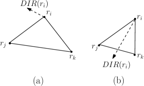
  Figure 11: An example of case 1 for lemma 5

• Case 2 (Two of the robots move):
  Without loss of generality, suppose $r_{i}$ and $r_{j}$ move while $r_{k}$ remains stationary. This case would be feasible only if $n\geq 4$.

  • Case 2.1:
    Suppose $r_{i}$ and $r_{j}$ move synchronously. Then by lemma 3.2,

    $$DISP(r_{i}r_{k})\leq\frac{\angle{r_{i}r_{k}r_{j}}}{n^{2}}$$ (4)

    And

    $$DISP(r_{j}r_{k})\leq\frac{\angle{r_{i}r_{k}r_{j}}}{n^{2}}$$ (5)

    From equation 4 and 5

    $$DISP(r_{i}r_{k})+DISP(r_{j}r_{k})<\angle{r_{i}r_{k}r_{j}}$$ (6)

    The minimum value of $DISP(r_{i}r_{k})+DISP(r_{j}r_{k})$ for which $r_{i},r_{j}$ and $r_{k}$ could become collinear is $\angle{r_{i}r_{k}r_{j}}$ . In view of equation $(\ref{r_ir_j})$, we conclude that $r_{i},r_{j}$ and $r_{k}$ would never become collinear.

  • Case 2.2:
    Suppose that $r_{i}$ is in motion and is at $\hat{r_{i}}^{\prime}$ when $r_{j}$ computes the value of $\Delta(r_{j})$. If $\hat{r_{i}}^{\prime}$ and $r_{j}$ lie in opposite sides of $\mathcal{L}_{r_{i}r_{k}}$ (Figure 12(a)),

    

    Figure 12: An example of case 2.2 for lemma 5

    then

    $$\Delta(r_{j})\leq\frac{1}{n^{2}}dist(r_{j},\mathcal{L}_{r_{k}\hat{r_{i}}^{\prime}})$$

    which implies that $r_{j}$ can not reach $\mathcal{L}_{r_{i}r_{k}}$ when $r_{i}$ reaches its destination and hence the lemma. Suppose $\hat{r_{i}}^{\prime}$ and $r_{j}$ lie in same side of $\mathcal{L}_{r_{i}r_{k}}$ (Figure 12(b)). Then we have,

    $$DISP(r_{i}r_{k}) \leq\frac{\angle{\hat{r_{i}}^{\prime}r_{k}r_{j}}}{n^{2}}$$

    $$<\frac{\angle{\hat{r_{i}}r_{k}r_{j}}}{n^{2}}$$

    Lemma follows from the same arguments as used in Case $2.1$.
    Consider the case: suppose $r_{j}$ takes the snapshot at time $t$ and moves to its destination at time $t^{\prime}$. In between times $t$ and $t^{\prime}$, suppose $r_{i}$ has made at most $\frac{n-1}{2}$ moves (we shall prove in case 3.2 that number of movements of any robot is bounded above by $\frac{n-1}{2}$). If $r_{i}$ moves towards $r_{j}$, after $\frac{n-1}{2}$ moves, we would have

    $$DISP(r_{i}r_{j})<(1-\frac{1}{n^{2}})^{\frac{n-1}{2}}\angle{r_{i}r_{k}r_{j}}$$

    which is less than $(1-\frac{1}{n^{2}})\angle{r_{i}r_{k}r_{j}}$. Hence equation $(\ref{r_ir_j})$ is satisfied in this case and we have the proof of the lemma. If $r_{i}$ moves away from $r_{j}$, then there is nothing to prove.

• Case 3 (All three robots move):

  • Case 3.1:
    Suppose $r_{i},r_{j}$ and $r_{k}$ move synchronously.

  • Case 3.1.1:
    Suppose $\mathcal{L}_{\hat{r}_{i}\hat{r}_{j}}$ intersects $\mathcal{L}_{r_{i}r_{j}}$ at an angle $\phi>0$ (Figure 13).

    

    Figure 13: An example of case 3.1.1 for lemma 5

    By lemma 3.4,

    $$\phi <2Max\{\theta(r_{i}),\theta(r_{j})\}$$

    $$\leq\frac{2}{n^{2}}\angle{r_{i}r_{j}r_{k}}$$ (7)

    In $\triangle{ABr_{j}}$,

    $$\psi =\angle{r_{i}r_{j}r_{k}}-\phi$$

    $$>\angle{r_{i}r_{j}r_{k}}-\frac{2}{n^{2}}\angle{r_{i}r_{j}r_{k}}$$

    $$=\frac{n-2}{n^{2}}\angle{r_{i}r_{j}r_{k}}$$

    $$\geq\frac{3}{5^{2}}\angle{r_{i}r_{j}r_{k}}$$ (8)

    Now $r_{i}$, $r_{j}$ and $r_{k}$ would be collinear only if

    $$DISP(r_{k}B) =\psi$$ (9)

    From lemma 3.6,

    $$DISP(r_{k}B) <DISP(r_{k}\hat{r}_{j})$$

    $$<2Max\{\theta(r_{i}),\theta(r_{j})\}$$

    $$\leq\frac{2}{5^{2}}\angle{r_{i}r_{j}r_{k}}$$ (10)

    Equations – ‣ • ‣ 3.9, 9 and – ‣ • ‣ 3.9 imply that $r_{i}$, $r_{j}$ and $r_{k}$ do not become collinear.

  • Case 3.1.2:
    Suppose $\mathcal{L}_{\hat{r}_{i}\hat{r}_{j}}$ and $\mathcal{L}_{r_{i}r_{j}}$ are parallel i.e., $\phi=0$ which implies that $\psi=\angle{r_{i}r_{j}r_{k}}$ (Figure 14). Let $Bisec(r_{k})$ intersect $\mathcal{L}_{r_{i}r_{j}}$ at $P$ and $|\overline{r_{k}P}|=l$. Since $\Delta(r_{k})\leq|\overline{r_{i}r_{j}}|sin(\frac{\angle{r_{i}r_{j}r_{k}}}{n^{2}})$ and $n\geq 5$,

    

    Figure 14: An example of case 3.1.2 for lemma 5

    $$l-\Delta(r_{k}) \geq|\overline{r_{i}r_{j}}|sin(\angle{r_{i}r_{j}r_{k}})-\Delta(r_{k})$$

    $$\geq|\overline{r_{i}r_{j}}|sin(\angle{r_{i}r_{j}r_{k}})-|\overline{r_{i}r_{j}}|sin(\frac{\angle{r_{i}r_{j}r_{k}}}{n^{2}})$$

    $$\geq|\overline{r_{i}r_{j}}|(sin(\angle r_{i}r_{j}r_{k})-sin(\frac{\angle{r_{i}r_{j}r_{k}}}{5^{2}}))$$

    $$>|\overline{r_{i}r_{j}}|sin(\frac{\angle{r_{i}r_{j}r_{k}}}{5^{2}})$$ (11)

    $\Delta(r_{i})$ and $\Delta(r_{j})$ are bounded above by $|\overline{r_{i}r_{j}}|sin$ $(\frac{\angle{r_{i}r_{j}r_{k}}}{5^{2}})$. Hence by equation $(\ref{eq-11})$, $r_{i}$ and $r_{j}$ and $r_{k}$ do not become collinear.

• Case 3.2:

  Suppose $r_{i}$, $r_{j}$ and $r_{k}$ move asynchronously. The main problem in this case is the following scenario: suppose $r_{j}$ or $r_{k}$ takes the snapshot at time $t_{j}$ or $t_{k}$ respectively and starts moving to its computed destination at time $t^{\prime}_{j}$ or $t^{\prime}_{k}$ respectively. Suppose the configuration has been changed in between the times due to the movements of the other robots. Then the corresponding $\Delta$ value of $r_{j}$ or $r_{k}$ is not consistent w.r.t. the current configuration. We have to show that this would not create any problem for our algorithm. The main idea of proof in this case is that we have to estimate the maximum amount of inclination of $\mathcal{L}_{r_{i}r_{j}}$ towards $r_{k}$ between the times $r_{j}$ or $r_{k}$ takes the snapshot of surroundings and it reaches the destination. So, in the following proofs we only consider the scenarios (as in the case 3.1.1. and case 3.1.2) in which there are possibilities of maximum reduction in the $\angle{r_{i}r_{j}r_{k}}$, which depicts the inclination of $\mathcal{L}_{r_{i}r_{j}}$ towards $r_{k}$. Note that the inclination of $\mathcal{L}_{r_{i}r_{j}}$ towards $r_{k}$ is maximum when both $r_{i}$ and $r_j$

References

- [1] C. Agathangelou, C. Georgiou, and M. Mavronicolas. A distributed algorithm for gathering many fat mobile robots in the plane. In Proceedings of the 32nd ACM Symposium on Principles of Distributed Computing (PODC), 250–259, 2013.
- [2] G. Antonio Di Luna, P. Flocchini, S. Gan Chaudhuri, N. Santoro, and G. Viglietta. Robots with Lights: Overcoming Obstructed Visibility Without Colliding In Proc. 16th International Symposium on Stabilization, Safety, and Security of Distributed Systems (SSS’14), to appear.
- [3] G. Antonio Di Luna, P. Flocchini, F. Poloni,, N. Santoro, and G. Viglietta. The Mutual Visibility Problem for Oblivious Robots. In Proc. 26th Canadian Conference on Computational Geometry (CCCG’14), to appear.
- [4] K. Bolla, T. Kovacs, and G.Fazekas. Gathering of fat robots with limited visibility and without global navigation. In Int. Symp. on Swarm and Evolutionary Comp., 30–38, 2012.
- [5] R.Cohen and D.Peleg. Local spreading algorithms for autonomous robot systems. Theoretical Computer Science, 399:71–82, 2008.
- [6] J. Czyzowicz, L. Gasieniec, and A. Pelc. Gathering few fat mobile robots in the plane. Theoretical Computer Science, 410(6â7):481 – 499, 2009.
- [7] S. Das, P. Flocchini, G. Prencipe, N. Santoro, and M. Yamashita. The power of lights: Synchronizing asynchronous robots using visible bits. In Proceedings of the 32nd International Conference on Distributed Computing Systems (ICDCS), 506–515, 2012.
- [8] S. Das, P. Flocchini, G. Prencipe, N. Santoro, and M. Yamashita. Synchronized dancing of oblivious chameleons. In Proc. 7th Int. Conf. on FUN with Algorithms (FUN), 2014.
- [9] A. Efrima and D. Peleg. Distributed models and algorithms for mobile robot systems. In Proceedings of the 33rd International Conference on Current Trends in Theory and Practice of Computer Science (SOFSEM), 70–87, 2007.
- [10] P. Flocchini, G. Prencipe, and N. Santoro. Distributed Computing by Oblivious Mobile Robots. Morgan & Claypool, 2012.
- [11] P. Flocchini, N. Santoro, G. Viglietta, and M. Yamashita. Rendezvous of two robots with constant memory. In Proceedings of the 20th International Colloquium on Structural Information and Communication Complexity (SIROCCO), 189–200, 2013.
- [12] D. Peleg. Distributed coordination algorithms for mobile robot swarms: New directions and challenges. In Proc. 7th Int. Workshop on Distr. Comp. (IWDC), 1–12, 2005.
- [13] G. Viglietta. Rendezvous of two robots with visible bits. In Proc. 9th Symp. on Algorithms and Experiments for Sensor Systems, Wireless Networks and Distributed Robotics (ALGOSENSORS), 291–306, 2013.