Chiral asymmetry in cold QED plasma in a strong magnetic field

Abstract

The interaction induced chiral asymmetry is calculated in cold QED plasma beyond the weak-field approximation. By making use of the recently developed Landau-level representation for the fermion self-energy, the chiral shift and the parity-even chiral chemical potential function are obtained with the help of numerical methods. The results are used to quantify the chiral asymmetry of the Fermi surface in dense QED matter. Because of the weakness of the QED interactions, the value of the asymmetry appears to be rather small even in the strongest magnetic fields and at the highest stellar densities. However, the analogous asymmetry can be substantial in the case of dense quark matter.

I Introduction

Nowadays the studies of chiral asymmetry in magnetized relativistic matter has drawn attention of researchers across diverse areas in physics. Heavy-ion collisions Kharzeev1 ; Kharzeev2 ; Liao , compact stars Charbonneau ; Ohnishi , the early Universe Giovannini:1997eg ; Boyarsky:2011uy ; Tashiro:2012mf , and Dirac/Weyl semimetals Turner ; Vafek are the main physical systems where such studies are relevant. The principal role in generating a chiral asymmetry in relativistic matter with usual vectorlike gauge interactions is played by an external magnetic field $\mathbf{B}$. In fact, it is the lowest Landau level (LLL) that is primarily responsible for the generation of chiral asymmetry in magnetized relativistic matter. The LLL is special because it has fermion spins completely polarized: they are directed along the magnetic field for a positive charge and opposite to the field for a negative one. For massless or ultrarelativistic particles, it is more appropriate to talk about their helicity rather than spin. Since the helicity of massless particles is the same as their chirality and the chiralities of the left- and right-handed particles are opposite, it is easy to understand how a nondissipative axial current $\mathbf{j}_{5}=e\mathbf{B}\mu/(2\pi^{2})$ is generated in magnetized relativistic fermion matter at nonzero chemical potential $\mu$ Vilenkin . This result is known in the literature as the chiral separation effect (CSE) (see, e.g., Ref. Fukushima ) and only the lowest Landau level contributes to the axial current in the free theory Zhitnitsky .

The chiral magnetic effect (CME) Kharzeev:2007jp ; Fukushima:2008xe is in a sense a dual phenomenon to the chiral separation effect. The CME implies that the chiral asymmetry in magnetized relativistic matter, e.g., described by a nonvanishing chiral chemical potential $\mu_{5}\neq 0$, causes a nondissipative electric current $\mathbf{j}=e^{2}\mathbf{B}\mu_{5}/(2\pi^{2})$. (See, however, the recent holographic study in Ref. Jimenez-Alba:2014iia , which points some fundamental differences between the realization of the CME and CSE.) Moreover, an interplay of the chiral separation and chiral magnetic effects gives rise to a novel type of collective gapless excitations: the chiral magnetic wave (CMW) CMW1 . Indeed, according to the CSE, a local fluctuation of the electric charge density induces a local fluctuation of the axial current. The resulting fluctuation of the chiral chemical potential produces a local fluctuation of the electric current via the CME. The latter in turn leads again to a local fluctuation of electric charge density and thus provides a self-sustaining mechanism for the propagation of a chiral magnetic wave. In heavy-ion collisions, such a wave leads to the quadrupole CME chiral-shift-2 ; CMW2 . One of the observable implications of the latter is the splitting of the elliptic flows of positively and negatively charged pions, i.e., $v^{\pi^{-}}_{2}-v^{\pi^{+}}_{2}=r_{e}A$, where $A$ is the net charge asymmetry $A=(\bar{N}^{+}-\bar{N}^{-})/(\bar{N}^{+}+\bar{N}^{-})$ and $r_{e}$ is the slope parameter CMW2 . Such a splitting was observed by the STAR collaboration Adamczyk:2013kcb ; Wang:2012qs ; Ke:2012qb and appears to be in agreement with theoretical predictions.

Apart from the CSE and CME, there also exist other related anomalous transport phenomena, e.g., the chiral vortical effect (CVE) CVE1 ; CVE2 ; CVE3 ; CVE4 , the chiral electric effect (CEE) Neiman , and the chiral charge generation effect (CCGE) Minwalla ; Melgar . In the free theory, these effects can be directly deduced from the chiral and gravitational anomalies. The chiral anomaly anomaly describes the violation of the classically conserved chiral symmetry at the quantum level. It should be noted that in the presence of an external magnetic field the chiral anomaly is generated entirely on the lowest Landau level Ambjorn . It is essential that the operator relation for the chiral anomaly is one-loop exact and cannot get any higher-order radiative corrections Bardeen . Since the chiral anomalous effects in the free theory are generated by the quantum anomalies, it was argued in Refs. Zhitnitsky ; Newman that the one-loop results for the anomalous transport coefficients should be exact. One should keep in mind, however, that in order to get these anomalous transport coefficients one should calculate the ground state expectation values of the corresponding operator relations. Therefore, a priori there is no guarantee that interaction corrections should be absent.

The first studies of the interaction effects were done in Refs. chiral-shift-1 ; Ruggieri ; chiral-shift-3 in the framework of the dense Nambu–Jona-Lasinio (NJL) model in a magnetic field. Using the method of Schwinger–Dyson equation for the fermion propagator, it was found that the interaction between the fermions in LLL and higher Landau levels promotes the chiral asymmetry from the LLL to all Landau levels chiral-shift-2 . For a magnetic field directed along the positive $z$-axis, dynamically generated chiral shift parameter $\Delta$ enters the effective action as the $\Delta\bar{\psi}\gamma^{3}\gamma^{5}\psi$ term and produces an additional dynamical contribution to the axial current. It should be emphasized that since this term does not break any symmetry in dense relativistic matter in a magnetic field, the chiral shift is already generated in the perturbation theory chiral-shift-1 ; chiral-shift-2 . In the NJL model the chiral shift takes a constant value independent of the momentum and the Landau level index. In the chiral limit, it determines the relative shift of the momenta in the dispersion relations of opposite chirality fermions $k^{3}\to k^{3}\pm\Delta$, where the momentum $k^{3}$ is directed along the magnetic field. In other words, it splits the Dirac point into two Weyl nodes separated in momentum space by $2\Delta$. It was proposed, therefore, that the same mechanism should take place in Dirac semimetals at nonzero charge density: in a magnetic field they transform into Weyl semimetals engineering .

Direct quantum-field theoretical calculations performed in dense QED to the leading order in coupling and the external magnetic field radiative-corrections showed that the axial current in the CSE receives nontrivial radiative corrections. It was found that, in the weak-field limit, the radiative corrections to the CSE originate from the singularities at the Fermi surface. (The radiative corrections to the chiral vorticity conductivity connected with the CVE were calculated in Refs. Golkar ; Ren .) The role of the interaction effects and radiative corrections in various chiral anomalous effects in magnetized relativistic matter were recently discussed in Refs. Jansen ; Zakharov .

By calculating the electron self-energy in magnetized QED plasma to the leading order in the coupling constant and the external magnetic field, it was found in Ref. chiral-shift-QED that the chiral asymmetry of the normal ground state of the system is characterized by two distinct Dirac structures. While one of them is the chiral shift familiar from the NJL model studies, the other Dirac structure is new. It formally looks like that of the chiral chemical potential but is an odd function of the longitudinal component of the momentum (i.e., directed along the magnetic field). The origin of this new parity-even chiral structure is directly connected with the long-range character of the QED interaction. The calculations in Ref. chiral-shift-QED were performed in the weak magnetic field approximation, using the pseudomomentum representation. Recently, the same pseudomomentum representation was also tested in the problem of chiral symmetry breaking in QCD at zero baryon density Watson:2013ghq .

The calculation of the fermion self-energy (as well as the chiral asymmetry functions) in the weak-field limit chiral-shift-QED revealed an infrared logarithmic singularity. This feature may well be an artifact of the expansion in powers of the magnetic field. It may also be related to yet another problem. As shown in Ref. radiative-corrections , the weak-field result for the axial current density depends on the photon mass which is introduced as an infrared regulator. It was argued, however, that such a dependence is fictitious and is expected to go away after taking into account the nonperturbative corrections beyond the weak-field limit. As a first step in the direction of resolving the limitations of the weak-field expansion chiral-shift-QED , in this paper we study the fermion self-energy and chiral asymmetry in cold magnetized QED plasma in the Landau level representation.

This paper is organized as follows. In Sec. II, we briefly introduce the model and notations. The definition of the fermion self-energy and its Landau-level representation are reviewed in Sec. III. In the same section, we also define the chiral asymmetry functions and discuss their ultraviolet properties. The numerical algorithm for calculating the chiral asymmetry functions, as well as the main results are presented in Sec. IV. In Sec. V, we summarize our findings and give our conclusions. In several appendices at the end of the paper, we provide some technical details and derivations used in the main text.

II Model

Following closely the notation of Ref. chiral-shift-QED , we start from the following Lagrangian density of QED in an external magnetic field:

$${\cal L}=-\frac{1}{4}F^{\mu\nu}F_{\mu\nu}+\bar{\psi}\left(i\gamma^{\nu}{\cal D}_{\nu}+\mu\gamma^{0}-m\right)\psi,$$ (1)

where ${\cal D}_{\nu}=\partial_{\nu}-ieA^{\rm ext}_{\nu}-ieA_{\nu}$ is the covariant derivative, $\mu$ is the fermion chemical potential, and $m$ is the bare fermion mass. Note that the notation is similar to that of Ref. Peskin , but assumes the opposite sign of the electric charge $e$, i.e., our $e$ is positive. Without loss of generality, we assume that the external magnetic field $\mathbf{B}$ points in the $z$ direction. The components of the spatial vectors, including those of the vector potential $\mathbf{A}^{\rm ext}$, are identified with the contravariant components. The components of the gradient $\bm{\nabla}$ are given by $\partial_{k}\equiv-\partial^{k}$. When the explicit form of the vector potential is needed, we utilize the Landau gauge, $\mathbf{A}^{\rm ext}=(0,xB,0)$.

In the presence of a constant magnetic field $\mathbf{B}$, part of the translational symmetry in the system is broken. This is obvious because, for one-particle states of charged fermions, the momentum perpendicular to the magnetic field is not a good quantum number. The absence of the translational invariance is reflected in the structure of the fermion propagator Schwinger:1951nm , i.e.,

$$S(u,u^{\prime})=e^{i\Phi(\mathbf{r},\mathbf{r}^{\prime})}\bar{S}(u-u^{\prime}),$$ (2)

where $u=(t,\mathbf{r})$ is a space-time four-vector, $\mathbf{r}=(x,y,z)$, $\Phi(\mathbf{r},\mathbf{r}^{\prime})=-eB(x+x^{\prime})(y-y^{\prime})/2$ is the Schwinger phase, and $\bar{S}(u-u^{\prime})$ is the translation invariant part of the propagator. A similar form is valid for the inverse fermion propagator as well chiral-shift-QED , i.e.,

$$S^{-1}(u,u^{\prime})=e^{i\Phi(\mathbf{r},\mathbf{r}^{\prime})}\bar{S}^{-1}(u-u^{\prime}).$$ (3)

It should be emphasized, though, that the translation invariant part $\bar{S}^{-1}(u-u^{\prime})$ is not the inverse of $\bar{S}(u-u^{\prime})$.

III Fermion self-energy

As proposed in the previous study chiral-shift-QED , the chiral asymmetry of the dense QED in a magnetic field is captured by the structure of the fermion self-energy. To leading order in coupling constant $\alpha=e^{2}/(4\pi)$, the corresponding expression for the self-energy in coordinate space reads

$$\Sigma(u,u^{\prime})=-4i\pi\alpha\gamma^{\mu}S(u,u^{\prime})\gamma^{\nu}D_{\mu\nu}(u-u^{\prime}).$$ (4)

By taking into account the structure of the propagator in Eq. (2), we find that the self-energy has the same Schwinger phase factor, i.e., $\Sigma(u,u^{\prime})=e^{i\Phi(\mathbf{r},\mathbf{r}^{\prime})}\bar{\Sigma}(u-u^{\prime})$. After dropping the corresponding phase on both sides of Eq. (4) and performing the Fourier transform, we arrive at the following pseudomomentum representation for the translation invariant part of the self-energy:

$$\bar{\Sigma}(p)=-4i\pi\alpha\int\frac{dk_{0}dk_{3}d^{2}\mathbf{k}_{\perp}}{(2\pi)^{4}}\gamma^{\mu}\bar{S}(k)\gamma^{\nu}D_{\mu\nu}(k-p).$$ (5)

Here $\bar{S}(k)$ is the Fourier transform of the translation invariant part of the fermion propagator, and $D_{\mu\nu}(q)$ is the momentum space representation for the photon propagator.

In the study at hand, we are interested in properties of cold QED matter at nonzero density. Moreover, we assume that the fermion number density is large, i.e., the corresponding value of the chemical $\mu$ is much larger than other energy scales in the problem. In particular, we assume that $\mu\gg\sqrt{|eB|}\gg m$, which is a reasonable hierarchy, for example, in the case of electron plasma in magnetars. One of the most important effects associated with the nonzero density is the screening of the one-photon exchange interaction. Even at weak coupling, such screening is strong and plays an important role in the dynamics. The well-known scheme that captures the corresponding effects is called the hard-dense-loop (HDL) approximation Vija ; Manuel . The explicit form of the HDL photon propagator in Euclidean space is given by

$$D_{\mu\nu}(q)\simeq i\left(\frac{|\bm{q}|}{|\bm{q}|^{3}+\frac{\pi}{4}m_{D}^{2}|q_{4}|}O^{\rm(mag)}_{\mu\nu}+\frac{O^{\rm(el)}_{\mu\nu}}{q_{4}^{2}+|\bm{q}|^{2}+m_{D}^{2}}\right),$$ (6)

where $q_{4}\equiv iq_{0}$ and $m_{D}^{2}=2\alpha\mu^{2}/\pi$ is the Debye screening mass. In the Coulomb gauge assumed here, the Lorentz space projectors onto the electric and magnetic modes are defined as follows:

$$O^{\rm(mag)}_{\mu\nu} = g_{\mu\nu}-u_{\mu}u_{\nu}+\frac{\bm{q}_{\mu}\bm{q}_{\nu}}{|\bm{q}|^{2}},$$ (7)

$$O^{\rm(el)}_{\mu\nu} = u_{\mu}u_{\nu},$$ (8)

where $u_{\mu}=(1,0,0,0)$.

The explicit form of the translation invariant part of the free fermion propagator is given by Chodos:1990vv

$$\bar{S}(k)=2ie^{-k_{\perp}^{2}l^{2}}\sum_{n=0}^{\infty}\frac{(-1)^{n}D_{n}(k)}{[k_{0}+\mu+i\epsilon\,\mbox{sgn}(k_{0})]^{2}-2n|eB|-(k^{3})^{2}-m^{2}},$$ (9)

where $l\equiv 1/\sqrt{|eB|}$ is the magnetic length and

$$D_{n}(k) = \left[\gamma^{0}(k_{0}+\mu)-\gamma^{3}k^{3}+m\right]\left[L_{n}\left(2k_{\perp}^{2}l^{2}\right){\cal P}_{-}-L_{n-1}\left(2k_{\perp}^{2}l^{2}\right){\cal P}_{+}\right]+2(\bm{\gamma}_{\perp}\cdot\mathbf{k}_{\perp})L^{1}_{n-1}\left(2k_{\perp}^{2}l^{2}\right).$$ (10)

Here ${\cal P}_{\pm}=\left[1\pm i\,\mbox{sgn}(eB)\gamma^{1}\gamma^{2}\right]/2$ are spin projectors and $L^{(\alpha)}_{n}(x)$ are generalized Laguerre polynomials Gradstein_Ryzhik . By definition, $L_{-1}(x)=0$.

The structure of the one-loop self-energy (5) was discussed in detail in Ref. chiral-shift-QED by utilizing the Landau-level representation, recently developed in Ref. Gorbar:2011kc . Just like the fermion propagator in Eqs. (9) and (10), the self-energy can be expanded over the Landau levels. The corresponding general form reads

$$\bar{\Sigma}(p) = 2e^{-p_{\perp}^{2}l^{2}}\sum_{n=0}^{\infty}(-1)^{n}\Big{\{}\left(-\gamma^{0}\delta\mu_{n}+p^{3}\gamma^{3}\delta v_{3,n}-i\gamma^{1}\gamma^{2}\tilde{\mu}_{n}-\gamma^{3}\gamma^{5}\Delta_{n}-\gamma^{0}\gamma^{5}\mu_{5,n}+{\cal M}_{n}\right)$$ (11)

$$\times\left[L_{n}(2p_{\perp}^{2}l^{2}){\cal P}_{-}-L_{n-1}(2p_{\perp}^{2}l^{2}){\cal P}_{+}\right]-2(\bm{\gamma}_{\perp}\cdot\bm{p}_{\perp}){\delta v_{\perp,n}}L^{1}_{n-1}(2p_{\perp}^{2}l^{2})\Big{\}}.$$

In this representation, the physical meaning of the coefficient functions $\delta\mu_{n}$, $\delta v_{3,n}$, etc., is obvious from their Dirac structure chiral-shift-QED . [Note that all these functions depend on the energy $p_{0}$ and the longitudinal momentum $p_{3}$.] In the remainder of this study, however, we will concentrate only on the two most important structures, $\Delta_{n}(p_{3})$ and $\mu_{5,n}(p_{3})$ at $p_{0}=0$, which describe the chiral asymmetry of dense QED matter. General expressions for both of these were derived in Ref. chiral-shift-QED by projecting the self-energy in Eq. (5) onto individual Landau levels, i.e.,

$$\Delta_{n}(p_{3}) = \frac{(-1)^{n}}{8}\frac{l^{2}}{\pi}\mathrm{sign}(eB)\int d^{2}\mathbf{p}_{\perp}e^{-p^{2}_{\perp}l^{2}}\left[L_{n}(2p_{\perp}^{2}l^{2})+L_{n-1}(2p_{\perp}^{2}l^{2})\right]\mathrm{Tr}\left[\gamma^{0}\bar{\Sigma}(p)\right]$$ (12)

$$- \frac{(-1)^{n}}{8}\frac{l^{2}}{\pi}\int d^{2}\mathbf{p}_{\perp}e^{-p^{2}_{\perp}l^{2}}\left[L_{n}(2p_{\perp}^{2}l^{2})-L_{n-1}(2p_{\perp}^{2}l^{2})\right]\mathrm{Tr}\left[\gamma^{3}\gamma^{5}\bar{\Sigma}(p)\right],$$

and

$$\mu_{5,n}(p_{3}) = \frac{(-1)^{n}}{8}\frac{l^{2}}{\pi}\mathrm{sign}(eB)\int d^{2}\mathbf{p}_{\perp}e^{-p^{2}_{\perp}l^{2}}\left[L_{n}(2p_{\perp}^{2}l^{2})+L_{n-1}(2p_{\perp}^{2}l^{2})\right]\mathrm{Tr}\left[\gamma^{3}\bar{\Sigma}(p)\right]$$ (13)

$$+ \frac{(-1)^{n}}{8}\frac{l^{2}}{\pi}\int d^{2}\mathbf{p}_{\perp}e^{-p^{2}_{\perp}l^{2}}\left[L_{n}(2p_{\perp}^{2}l^{2})-L_{n-1}(2p_{\perp}^{2}l^{2})\right]\mathrm{Tr}\left[\gamma^{0}\gamma^{5}\bar{\Sigma}(p)\right],$$

respectively.

At large chemical potential considered here, magnetic catalysis Gusynin:1995gt plays no role and the dynamical contribution to ${\cal M}_{n}$ is negligible even compared to the electron mass $m_{e}$. It is completely justifiable, therefore, to replace ${\cal M}_{n}$ with $m$ in our calculations below. Moreover, the dynamical contribution to the electron mass due to the magnetic catalysis in QED is exponentially small even in the case of zero chemical potential (vacuum) Gusynin:1995gt ; Leung:1996qy ; Gusynin:1998zq . This is the consequence of the smallness of the fine structure constant. While the same is not true in the QCD vacuum, the magnetic catalysis still would not play any big role in dense quark matter at large chemical potential.

Before proceeding to the numerical analysis of the chiral asymmetry functions $\Delta_{n}(p_{3})$ and $\mu_{5,n}(p_{3})$, let us discuss the implications of the well-known ultraviolet divergency in the fermion self-energy function in QED Peskin . In the Pauli-Villars regularization scheme, the self-energy contains the following logarithmically divergent contribution Peskin :

$$\Sigma^{\rm(div)}(p)=\frac{\alpha}{4\pi}\left[-\gamma^{\nu}(p_{\nu}+\mu\delta_{\nu}^{0})+4m\right]\ln\frac{\Lambda^{2}}{m^{2}}.$$ (14)

Note that the only effect of a nonzero chemical potential here is to shift $p_{0}\to p_{0}+\mu$ in the vacuum expression radiative-corrections ; Freedman:1976xs . Of course, the above divergency cannot be affected by the magnetic field. When projected onto Landau levels as prescribed by Eqs. (12) and (13), this result leads to the following contributions to the chiral asymmetry functions:

$$\Delta^{\rm(div)}_{n}(p_{3}) = -\delta_{n}^{0}\frac{\alpha(p_{0}+\mu)}{8\pi}\mathrm{sign}(eB)\ln\frac{\Lambda^{2}}{m^{2}},$$ (15)

$$\mu^{\rm(div)}_{5,n}(p_{3}) = \delta_{n}^{0}\frac{\alpha p_{3}}{8\pi}\mathrm{sign}(eB)\ln\frac{\Lambda^{2}}{m^{2}}.$$ (16)

As we see, the corresponding functions are free of the ultraviolet divergences in all, but the lowest Landau level ($n=0$). As explained in detail in Ref. chiral-shift-QED , the LLL ($n=0$) is very special also because of its spin-polarized nature. As a consequence, the LLL chiral shift is indistinguishable from the correction to the chemical potential, and the LLL axial chemical potential is indistinguishable from the correction to the longitudinal velocity. It was concluded, therefore, that the novel type of the chiral asymmetry is determined exclusively by the dynamical functions $\Delta_{n}$ and $\mu_{5,n}$ with $n\geq 1$. These functions are of prime interest for us in the present paper. In the next section, we take into account that all these functions are free from the ultraviolet divergences and study them numerically.

IV Numerical results for chiral asymmetry

In this section we study the chiral asymmetry functions $\Delta_{n}(p_{3})$ and $\mu_{5,n}(p_{3})$ using numerical methods. To start with, we rewrite the corresponding expressions in a dimensionless form. We will measure all quantities with the dimension of energy/mass in terms of the chemical potential. For example, in the case of momenta, we will define the corresponding dimensionless quantities as follows: $x\equiv p_{\perp}/\mu$, $y\equiv k_{\perp}/\mu$, $x_{3}\equiv p_{3}/\mu$, and $y_{3}\equiv k_{3}/\mu$. Similarly, the dimensionless functions will be defined as follows: $\bar{\Delta}_{n}\equiv\Delta_{n}/\mu$ and $\bar{\mu}_{5,n}\equiv\mu_{5,n}/\mu$. The corresponding dimensionless forms of these chiral asymmetry functions are presented in Appendix B.

In order to analyze numerically the two chiral asymmetry functions in dense QED, we need to fix several model parameters (i.e., the strength of magnetic field, the value of the chemical potential, and the fermion mass). In principle, when using the dimensionless description, the value of the chemical potential $\mu$ may be left unspecified. Keeping in mind, however, that the value of the fermion (electron) mass has to be measured in units of $\mu$, we will assume that the default choices of the chemical potential and the magnetic field are $\mu=420~{}\mbox{MeV}$ and $B=10^{18}~{}\mbox{G}$. Then, the two dimensionless model parameters used in the calculations will be

$$a = \frac{m}{\mu}\approx 1.22\times 10^{-3}\frac{m}{m_{e}}\frac{420~{}\mbox{MeV}}{\mu},$$ (17)

$$b = \frac{|eB|}{\mu^{2}}\approx\frac{1}{30}\left(\frac{B}{10^{18}~{}\mbox{G}}\right)\left(\frac{420~{}\mbox{MeV}}{\mu}\right)^{2}.$$ (18)

Note that, in agreement with the assumption made earlier, the chosen value of the magnetic field strength is rather small compared to the chemical potential scale $\mu^{2}$. By taking into account the definition of the Debye mass and the QED fine structure constant, it is also convenient to introduce the following short-hand notation for the dimensionless Debye mass:

$$d=\frac{m_{D}}{\mu}\equiv\sqrt{\frac{2\alpha}{\pi}}\approx 6.816\times 10^{-2}.$$ (19)

In the final expressions for the chiral asymmetry functions, there will be a need to sum over an infinite number of Landau levels. In the numerical calculations, however, the sums will be truncated at $n_{\rm max}=200$.

As is clear from the explicit expressions for the functions $\bar{\Delta}_{n}$ and $\bar{\mu}_{5,n}$ in Appendix B [see Eqs. (41) and (42), respectively], the numerical calculation for each of them reduces to performing four integrations: three integrations over the dimensionless momenta $x$, $y$ and $y_{3}$, and one over the angular coordinate $\phi$. Taking into account that $\bar{\Delta}_{n}$ and $\bar{\mu}_{5,n}$ also have an additional functional dependence on the longitudinal momentum $x_{3}\equiv p_{3}/\mu$, the corresponding task becomes rather expensive numerically.

Before proceeding to the actual results, let us briefly describe the algorithm that we use in the calculations. The four-dimensional integrals that define the chiral asymmetry functions have the following schematic form:

$$I=\int_{0}^{\infty}dx\int_{0}^{\infty}dy\int_{-\infty}^{\infty}dy_{3}\int_{0}^{2\pi}\frac{d\phi}{2\pi}f(x,y,y_{3},\phi).$$ (20)

In order to calculate such an integral, we will make use of the importance sampling Monte Carlo method Weinzierl:2000wd . In such a framework, the result of the integration is approximated by a weighted sum of contributions calculated at a large number of random points in the phase space, i.e.,

$$I_{N}=\frac{1}{N}\sum_{i=1}^{N}\frac{f(x^{i},y^{i},y_{3}^{i},2\pi u^{i})}{P_{1}(x^{i})P_{2}(y^{i})P_{3}(y_{3}^{i})}.$$ (21)

Having limited information about the angular dependence of the integrand function, we use the simplest uniform distribution of the random variable $u=\phi/(2\pi)$ on the interval from $0$ to $1$. The other three random number variables are distributed with the probability density functions $P_{1}(x)$, $P_{2}(y)$, and $P_{1}(y_{3})$, respectively. The specific choice of these functions will be explained momentarily. First, however, let us note that the statistical error of the Monte Carlo integration is given by the following estimator Weinzierl:2000wd :

$$\epsilon=\frac{1}{\sqrt{N}}\sqrt{\frac{1}{N}\sum_{i=1}^{N}\left(\frac{f(x^{i},y^{i},y_{3}^{i},2\pi u^{i})}{P_{1}(x^{i})P_{2}(y^{i})P_{3}(y_{3}^{i})}\right)^{2}-I_{N}^{2}}.$$ (22)

With increasing $N$, the Monte Carlo estimate $I_{N}$ may converge rather slowly to the true value $I$. This is where importance sampling can improve the situation. The key observation is that, for a fixed number of sampling points $N$, the result for the above statistical error depends on the random number distributions used. The error becomes smaller when the corresponding probability densities approximate closer the integrand function itself. The same condition determines when the fastest convergence of the Monte Carlo method is achieved.

While testing our numerical algorithm, we tried performing calculations with several different types of the functional forms for the random number distributions (e.g., Gaussian and gamma distributions) and examined a number of different choices of their parameters. In such tests, the least value of the estimator (22) was used as an indicator of the integration effectiveness. This allowed us to make an optimal choice of the random number distributions.

In the case of the perpendicular momenta variables $x$ and $y$, we ended up using the following gamma distribution:

$$P(x)=\frac{\beta^{\alpha}}{\Gamma(\alpha)}x^{\alpha-1}e^{-\beta x},$$ (23)

where the shape and scale parameters are $\alpha=1$ and $\beta=1.5$, respectively. Such a distribution appears indeed appropriate in the case of the integrand function that decreases exponentially with the perpendicular momenta. In order to generate gamma-distributed random numbers, we used the FORTRAN code written by Richard Chandler gamma-distribution .

As a quick examination of the explicit expressions for $\bar{\Delta}_{n}$ and $\bar{\mu}_{5,n}$ in Appendix B reveals, the dependence of their integrands on the longitudinal momentum $y_{3}$ is quite different from the dependence on $x$ and $y$. In particular, they have a power-law instead of exponential behavior at large $y_{3}$. Because of this, neither Gaussian nor gamma distributions were able to provide a quick convergence of the Monte Carlo integration. Instead, we used the Cauchy distribution with the following power-law probability density function for generating the longitudinal momentum variable $y_{3}$:

$$P_{3}(y_{3})=\frac{1}{\pi}\frac{1}{y_{3}^{2}+1}.$$ (24)

The random numbers with such a probability density are generated using the quantile function $y_{3}=\tan\left[\frac{\pi}{2}(2p-1)\right]$, where $p$ is a random number with the uniform distribution on the interval between $0$ and $1$.

Our numerical results for the chiral shift are summarized in Fig. 1. In the left panel, we show the dependence of the chiral shift $\Delta_{n}$ on the longitudinal momentum $y_{3}=p_{3}/\mu$ for several low-lying Landau levels. Since obtaining the complete functional dependence on $p_{3}$ is rather expensive numerically, we used only a moderately large number of sampling points, $N=2\times 10^{8}$ and calculated the results only for the first four lowest lying Landau levels. The common feature of the corresponding functions is the appearance of a maximum at an approximate location of the Fermi surface. In the free (weakly interacting) theory, this is determined by the following value of the longitudinal momentum: $p_{3}/\mu=\sqrt{1-2nb-a^{2}}$, where $a$ and $b$ are defined in Eqs. (17) and (18). In agreement with this expression, the location of the maximum of the chiral shift function in the $n$th Landau level $\Delta_{n}(p_{3})$ decreases with increasing $n$. At large values of the momentum $p_{3}$, the chiral shift function decreases and gradually approaches zero as expected.

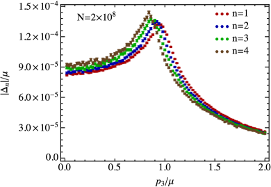
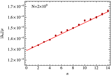
Figure 1: (color online) Left panel: the chiral shift $\Delta_{n}$ as a function of the longitudinal momentum $p_{3}$ for $n=1$ (red), $n=2$ (blue), $n=3$ (green), and $n=4$ (brown) Landau levels. Right panel: the values of the chiral shift $\Delta_{n}$ at the Fermi surface.

From the viewpoint of the low-energy physics, it is most important to know the chiral shift at the Fermi surface. The corresponding results are presented in the right panel of Fig. 1. By assumption, the location of the Fermi surface is determined by the perturbative expression, $p_{3}/\mu=\sqrt{1-2nb-a^{2}}$. In this calculation, we used a larger number of sampling points, $N=2\times 10^{9}$. As we see, the Fermi surface values of $\Delta_{n}$ grow with the Landau-level index $n$. (The corresponding numerical values are also given in the first column of Table 1.) This growth is somewhat surprising, but is in agreement with the general behavior of functions $\Delta_{n}(p_{3})$ shown in the left panel of Fig. 1. The corresponding dependence on the Landau-level index can be fitted quite well by a linear function.

It is easy to check that the numerical results for the chiral shift in Fig. 1 are of the same order of magnitude as $\alpha|eB|/\mu$. Taking into account that $\Delta_{n}$ is one of the structures in the fermion self-energy, induced by a nonzero magnetic field, it is indeed quite natural that the corresponding function is proportional to the coupling constant and the magnetic field strength. As for the chemical potential in the denominator, it is the only other relevant energy scale in the problem that can be used to render the result for $\Delta_{n}$ with the correct energy units. (Formally, the fermion mass is yet another energy scale, but it is unlikely to play a prominent role at the Fermi surface in the high density and strong-field limit.) The linear fit for the chiral shift at the Fermi surface is shown by the solid line in the right panel of Fig. 1. The corresponding function can be presented in the following form:

$$\Delta_{n}\simeq-\frac{\alpha|eB|}{\mu}\left(0.53+0.32\frac{|eB|n}{\mu^{2}}\right),$$ (25)

where we took into account that the numerical results in Fig. 1 were obtained for the magnetic field $|eB|=\mu^{2}/30$ and $\alpha=1/137$. The result in Eq. (25) should be contrasted with a very different parametric dependence obtained in the weak-field limit in Ref. chiral-shift-QED , i.e., $\Delta_{n}\propto\alpha|eB|\mu/m^{2}$, which is a factor of $(\mu/m)^{2}$ larger. Such a large factor is quite natural in the weak-field limit, where it is an artifact of the expansion in powers of $|eB|/m^{2}$. In contrast, one does not expect anything like that in the case of a strong magnetic field.

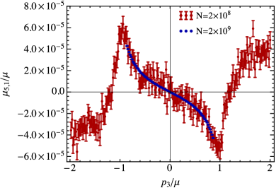
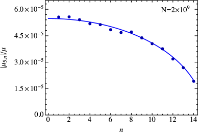
Figure 2: (color online) Left panel: the chiral chemical potential $\mu_{5,n}$ as a function of the longitudinal momentum $p_{3}$ for $n=1$ Landau level. Right panel: the values of the chiral chemical potential $\mu_{5,n}$ at the Fermi surface.

The numerical results for the chiral chemical potential $\mu_{5,n}$ are summarized in Fig. 2. In the left panel, we present the chiral chemical potential in the $n=1$ Landau level as a function of the longitudinal momentum $p_{3}$. (The results for larger $n$ are expected to have the same qualitative dependence on $p_{3}$.) The red and blue points represent the results for two different numbers of sampling points, $N=2\times 10^{8}$ and $N=2\times 10^{9}$, respectively. The numerical results confirm that $\mu_{5,n}$ is an odd function of $p_{3}$ and, as such, it does not break parity. The dependence of $\mu_{5,n}$ on $p_{3}$ also reveals a pair of sharp peaks on the Fermi surface at $p_{3}/\mu\simeq\pm\sqrt{1-2nb-a^{2}}$. In the context of the low-energy physics, it is these values of $\mu_{5,n}$ on the Fermi surface that are of main importance.

The numerical results for the chiral chemical potential at the Fermi surface are shown in the right panel of Fig. 2. In the corresponding calculation, we again assumed that the location of the Fermi surface is determined by the perturbative expression, $p_{3}/\mu=\pm\sqrt{1-2nb-a^{2}}$, and used the Monte Carlo integration algorithm with $N=2\times 10^{9}$ sampling points. We find that the values of $\mu_{5,n}$ decrease with the Landau-level index $n$. (The corresponding numerical values are given in the second column of Table 1.) The order of magnitude of the obtained results is similar to those for the chiral shift function. Following the same arguments, therefore, we can assume that $\mu_{5,n}$ is also proportional to the coupling constant and the magnetic field strengths, i.e., $\mu_{5,n}\propto\alpha|eB|/\mu$. (Let us emphasize again that this dependence is quite different from the weak-field limit in Ref. chiral-shift-QED .) In order to fit the numerical results, we could try to use a polynomial function of $n$. However, by following a trial and error approach instead, we found that the following simple function approximates our numerical results really well:

$$\mu_{5,n}\simeq-0.225\frac{\alpha|eB|}{\mu}\sqrt{1-\left(\frac{2n|eB|}{\mu^{2}}\right)^{2}},$$ (26)

where we took into account that $|eB|=\mu^{2}/30$ and $\alpha=1/137$. The corresponding function is shown by the solid line in the right panel of Fig. 2.

By making use of the analytical expression for the fermion propagator with the chiral asymmetry in Appendix A, as well as the above numerical results for the chiral shift and the chiral chemical potential, we can straightforwardly determine the interaction-induced deviations of the Fermi momenta $(p_{3}-p_{3}^{(0)})/\mu$ for the predominantly left-handed and right-handed fermions in the considered ultrarelativistic limit $\mu\gg m$. Here $p_{3}^{(0)}$ is the value of the Fermi momentum in the absence of the chiral asymmetry (i.e., $\Delta_{n}=0$ and $\mu_{5,n}=0$). Such deviations can be viewed as the actual measure of the chiral asymmetry at the Fermi surface. The numerical results for $(p_{3}-p_{3}^{(0)})/\mu$ in each occupied Landau level are shown in Fig. 3. (The corresponding numerical values are also presented in the last column of Table 1.) This is a generalization of the analogous results in the weak-field limit, obtained in Ref. chiral-shift-QED .

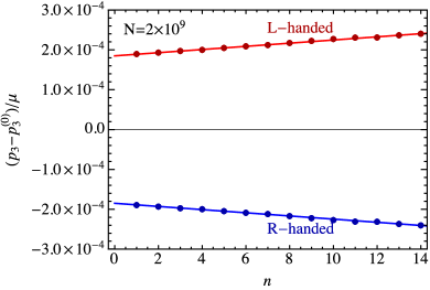
Figure 3: (color online) Asymmetry of the Fermi surface for predominantly left-handed (red) and right-handed (blue) particles as a function of the Landau-level index $n$.

We find that the results for $(p_{3}-p_{3}^{(0)})/\mu$ in Fig. 3 are well approximated by linear functions of $n$. When written in the same form as the chiral shift and the chiral chemical potential functions, the corresponding linear fits take the following form:

$$p_{3}-p_{3}^{(0)}\simeq\pm\frac{\alpha|eB|}{\mu}\left(0.76+0.49\frac{|eB|n}{\mu^{2}}\right).$$ (27)

As is easy to check, the values of these Fermi momenta shifts are of the order of $10$–$100~{}\mbox{keV}$ and, thus, are not very large in the context of compact stars, even though we already assumed an extremely strong value of the magnetic field, $B=10^{18}~{}\mbox{G}$. One should keep in mind, however, that here we used the model of a dense QED plasma, whose coupling constant $\alpha$ is extremely small. This conclusion could change drastically in the case of dense quark matter, where the relevant coupling constant $\alpha_{s}$ is about two orders of magnitude stronger. Indeed, by taking into account that the estimate for the Fermi momenta shift in Eq. (27) is proportional to the coupling, we conclude that the chiral asymmetry should be of the order of $1$–$10~{}\mbox{MeV}$ in dense quark matter. Such a large asymmetry may in turn produce a substantial neutrino emission asymmetry with observable consequences for protoneutron stars chiral-shift-2 .

V Discussion

In this paper, we studied the chiral asymmetry induced by a strong external magnetic field in cold dense QED matter. This study extends the general predictions of Ref. chiral-shift-QED regarding the structure of the chiral asymmetry at Fermi surface. Unlike the weak-field analysis of Ref. chiral-shift-QED , however, the present paper addressed the problem in the general framework that relies on the Landau-level representation. Additionally, the screening effects of dense plasma are taken into account in this study. This is done by utilizing the conventional hard-dense-loop approximation, which is justified in the regime considered.

Among the main results are the numerical functions for the chiral shift and the chiral chemical potential. The dependence of both functions on the longitudinal momentum reveals local peaks at the approximate position of the Fermi surface. This feature is in qualitative agreement with the perturbative weak-field results in Ref. chiral-shift-QED , where such functions had logarithmic singularities.

The values of the chiral shift $\Delta_{n}$ and the chiral chemical potential $\mu_{5,n}$ at the Fermi surface appear to be of order $\alpha|eB|/\mu$. This differs from the corresponding weak-field prediction $\alpha|eB|\mu/m^{2}$ by a rather large factor $(\mu/m)^{2}$. Such a difference is not surprising and, in fact, should have been expected in the ultrarelativistic limit when $|eB|/m^{2}$ is not a good expansion parameter. While the dependence of $\Delta_{n}$ on the Landau-level index $n$ shows a weak growth, $\mu_{5,n}$ decreases with $n$. By fitting the numerical results, we proposed simple model functions which describe the results quite well.

By making use of our numerical results for $\Delta_{n}$ and $\mu_{5,n}$, we also obtained the interaction induced deviations of the Fermi momenta $(p_{3}-p_{3}^{(0)})/\mu$ for the predominantly left-handed and right-handed fermions. These provide the formal measure of the chiral asymmetry at the Fermi surface. The corresponding values appear to be rather small in the case of dense QED matter even at extremely large densities and extremely strong magnetic fields. We suggest, however, that the asymmetry can be substantial in the case of quark matter.

Table 1: Data for the chiral asymmetry functions $\Delta_{n}$, $\mu_{5,n}$, and $(p_{3}-p_{3}^{(0)})/\mu$ at the Fermi surface.

$n$	$\Delta_{n}/\mu$	$\mu_{5,n}/\mu$	$(p_{3}-p_{3}^{(0)})/\mu$
1	$-1.32\times 10^{-4}\pm 1.84\times 10^{-7}$	$-5.56\times 10^{-5}\pm 3.30\times 10^{-7}$	$\pm 1.90\times 10^{-4}$
2	$-1.34\times 10^{-4}\pm 2.56\times 10^{-7}$	$-5.57\times 10^{-5}\pm 4.12\times 10^{-7}$	$\pm 1.93\times 10^{-4}$
3	$-1.37\times 10^{-4}\pm 3.21\times 10^{-7}$	$-5.41\times 10^{-5}\pm 4.64\times 10^{-7}$	$\pm 1.97\times 10^{-4}$
4	$-1.39\times 10^{-4}\pm 3.76\times 10^{-7}$	$-5.18\times 10^{-5}\pm 5.01\times 10^{-7}$	$\pm 2.00\times 10^{-4}$
5	$-1.43\times 10^{-4}\pm 4.34\times 10^{-7}$	$-5.13\times 10^{-5}\pm 5.27\times 10^{-7}$	$\pm 2.05\times 10^{-4}$
6	$-1.46\times 10^{-4}\pm 4.90\times 10^{-7}$	$-4.84\times 10^{-5}\pm 5.43\times 10^{-7}$	$\pm 2.09\times 10^{-4}$
7	$-1.48\times 10^{-4}\pm 5.46\times 10^{-7}$	$-4.68\times 10^{-5}\pm 5.52\times 10^{-7}$	$\pm 2.12\times 10^{-4}$
8	$-1.50\times 10^{-4}\pm 5.97\times 10^{-7}$	$-4.71\times 10^{-5}\pm 5.52\times 10^{-7}$	$\pm 2.17\times 10^{-4}$
9	$-1.53\times 10^{-4}\pm 6.54\times 10^{-7}$	$-4.38\times 10^{-5}\pm 5.42\times 10^{-7}$	$\pm 2.22\times 10^{-4}$
10	$-1.57\times 10^{-4}\pm 7.12\times 10^{-7}$	$-4.05\times 10^{-5}\pm 5.23\times 10^{-7}$	$\pm 2.27\times 10^{-4}$
11	$-1.58\times 10^{-4}\pm 7.53\times 10^{-7}$	$-3.76\times 10^{-5}\pm 4.94\times 10^{-7}$	$\pm 2.31\times 10^{-4}$
12	$-1.60\times 10^{-4}\pm 8.01\times 10^{-7}$	$-3.18\times 10^{-5}\pm 4.48\times 10^{-7}$	$\pm 2.31\times 10^{-4}$
13	$-1.63\times 10^{-4}\pm 8.47\times 10^{-7}$	$-2.69\times 10^{-5}\pm 3.83\times 10^{-7}$	$\pm 2.37\times 10^{-4}$
14	$-1.66\times 10^{-4}\pm 8.96\times 10^{-7}$	$-1.92\times 10^{-5}\pm 2.84\times 10^{-7}$	$\pm 2.40\times 10^{-4}$

Appendix A Fermion propagator with chiral asymmetry

The fermion propagator with the nonzero Dirac mass, chiral shift, and chiral chemical potential is formally defined by

$$G(u,u^{\prime})=i\langle u|\left[(i\partial_{t}+\mu)\gamma^{0}+\Delta\gamma^{3}\gamma^{5}+\mu_{5}\gamma^{0}\gamma^{5}-(\bm{\pi}_{\perp}\cdot\bm{\gamma})-\pi^{3}\gamma^{3}-m\right]^{-1}|u^{\prime}\rangle,$$ (28)

where $u=(t,\mathbf{r})$ is a space-time four-vector. By making use of this definition and utilizing the same method as in Ref. chiral-shift-2 , we straightforwardly show that the fermion propagator has the general structure as in Eq. (2) and the explicit form of the translation invariant part is determined by the following expression of its Fourier transform:

$$\bar{G}(\omega,\mathbf{k})=\int dtd^{3}\mathbf{r}e^{i\omega t-i(\mathbf{k}\cdot\mathbf{r})}\bar{G}(t;\mathbf{r})=ie^{-k_{\perp}^{2}l^{2}}\sum_{n=0}^{\infty}(-1)^{n}D_{n}(\omega,\mathbf{k})\frac{1}{\mathcal{M}-2n|eB|},$$ (29)

where $\mathbf{k}_{\perp}=(k^{1},k^{2})$, and the $n$th Landau level contribution is given in terms of the following matrix functions:

$$D_{n}(\omega,\mathbf{k}) = 2W\left[\mathcal{P}_{-}L_{n}(2k_{\perp}^{2}l^{2})-\mathcal{P}_{+}L_{n-1}(2k_{\perp}^{2}l^{2})\right]+4(\mathbf{k}_{\perp}\cdot\bm{\gamma})L^{1}_{n-1}(2k_{\perp}^{2}l^{2}),$$ (30)

$$W = (\omega+\mu)\gamma^{0}-\Delta\gamma^{3}\gamma^{5}-\mu_{5}\gamma^{0}\gamma^{5}-k^{3}\gamma^{3}+m,$$ (31)

$$\mathcal{M} = (\omega+\mu)^{2}-\Delta^{2}+\mu_{5}^{2}-{k_{3}}^{2}-m^{2}-2[\Delta k_{3}+(\omega+\mu)\mu_{5}]\gamma^{5}+2m\Delta\gamma^{3}\gamma^{5}+2m\mu_{5}\gamma^{0}\gamma^{5}.$$ (32)

Note that the last matrix factor in Eq. (29) can be rewritten in the following equivalent form:

$$\frac{1}{\mathcal{M}-2n|eB|}=\frac{\left[(\omega+\mu)^{2}-\Delta^{2}+\mu_{5}^{2}-{k_{3}}^{2}-m^{2}-2n|eB|\right]+2[\Delta k_{3}+(\omega+\mu)\mu_{5}]\gamma^{5}-2m\mu_{5}\gamma^{0}\gamma^{5}-2m\Delta\gamma^{3}\gamma^{5}}{\left[(\omega+\mu)^{2}-\Delta^{2}+\mu_{5}^{2}-{k_{3}}^{2}-m^{2}-2n|eB|\right]^{2}-4[\Delta k_{3}+(\omega+\mu)\mu_{5}]^{2}+4m^{2}\mu_{5}^{2}-4m^{2}\Delta^{2}},$$ (33)

which implies that the fermion dispersion relation in the presence of the chiral asymmetry is determined by the solutions to the equation:

$$\left[(\omega+\mu)^{2}-\Delta^{2}+\mu_{5}^{2}-{k_{3}}^{2}-m^{2}-2n|eB|\right]^{2}-4[\Delta k_{3}+(\omega+\mu)\mu_{5}]^{2}+4m^{2}\mu_{5}^{2}-4m^{2}\Delta^{2}=0.$$ (34)

Appendix B Chiral asymmetry functions in the HDL approximation

In this appendix, we present the explicit form of the chiral asymmetry functions $\Delta_{n}(p_{3})$ and $\mu_{5,n}(p_{3})$ in the approximation with the HDL photon propagator.

By making use of the definition in Eqs. (12) and (13), as well as the explicit form of the HDL photon propagator in Eq. (6), we derive the following results for the two coefficient functions of interest:

$$\Delta_{n}(p_{3}) = (-1)^{n}e^{2}l^{2}\mathrm{sign}(eB)\int\frac{dk_{3}d^{2}\mathbf{k}_{\perp}d^{2}\mathbf{p}_{\perp}}{(2\pi)^{4}}e^{-k_{\perp}^{2}l^{2}-p^{2}_{\perp}l^{2}}\displaystyle\sum_{N=0}^{\infty}(-1)^{N}$$ (35)

$$\Bigg{\{}\left[L_{n}(2p_{\perp}^{2}l^{2})+L_{n-1}(2p_{\perp}^{2}l^{2})\right]\left[L_{N}(2k_{\perp}^{2}l^{2})-L_{N-1}(2k_{\perp}^{2}l^{2})\right]\left(-\mathcal{D}^{\rm(mag)}+\frac{1}{2}\mathcal{D}^{\rm(el)}\right)$$

$$+\left[L_{n}(2p_{\perp}^{2}l^{2})-L_{n-1}(2p_{\perp}^{2}l^{2})\right]\left[L_{N}(2k_{\perp}^{2}l^{2})+L_{N-1}(2k_{\perp}^{2}l^{2})\right]\left(\frac{q_{3}^{2}}{|\bm{q}|^{2}}\mathcal{D}^{\rm(mag)}+\frac{1}{2}\mathcal{D}^{\rm(el)}\right)\Bigg{\}},$$

$$\mu_{5,n}(p_{3}) = (-1)^{n}e^{2}l^{2}\mathrm{sign}(eB)\int\frac{dk_{3}d^{2}\mathbf{k}_{\perp}d^{2}\mathbf{p}_{\perp}}{(2\pi)^{4}}e^{-k_{\perp}^{2}l^{2}-p^{2}_{\perp}l^{2}}\displaystyle\sum_{N=0}^{\infty}(-1)^{N}$$ (36)

$$\Bigg{\{}-\left[L_{n}(2p_{\perp}^{2}l^{2})+L_{n-1}(2p_{\perp}^{2}l^{2})\right]\left[L_{N}(2k_{\perp}^{2}l^{2})-L_{N-1}(2k_{\perp}^{2}l^{2})\right]k_{3}\left(\frac{q_{3}^{2}}{|\bm{q}|^{2}}\mathcal{F}^{\rm(mag)}+\frac{1}{2}\mathcal{F}^{\rm(el)}\right)$$

$$+\left[L_{n}(2p_{\perp}^{2}l^{2})-L_{n-1}(2p_{\perp}^{2}l^{2})\right]\left[L_{N}(2k_{\perp}^{2}l^{2})+L_{N-1}(2k_{\perp}^{2}l^{2})\right]k_{3}\left(\mathcal{F}^{\rm(mag)}-\frac{1}{2}\mathcal{F}^{\rm(el)}\right)$$

$$+4L^{1}_{N-1}(2k_{\perp}^{2}l^{2})\left[L_{n}(2p_{\perp}^{2}l^{2})+L_{n-1}(2p_{\perp}^{2}l^{2})\right]\frac{q_{3}(k_{1}q_{1}+k_{2}q_{2})}{|\bm{q}|^{2}}\mathcal{F}^{\rm(mag)}\Bigg{\}},$$

where the explicit expressions for the functions $\mathcal{D}^{\rm(mag)}$, $\mathcal{D}^{\rm(el)}$, $\mathcal{F}^{\rm(mag)}$, and $\mathcal{F}^{\rm(el)}$ are obtained after the integrations over $k_{0}\equiv i\omega_{E}$ performed, i.e.,

$$\mathcal{D}^{\rm(mag)} = \frac{i}{\pi}|\bm{q}|\int_{-\infty}^{\infty}\frac{(\omega_{E}-i\mu)d\omega_{E}}{\left[(\omega_{E}-i\mu)^{2}+\mathcal{M}^{2}_{N}\right]\left(|\bm{q}|^{3}+\frac{\pi}{4}m_{D}^{2}|\omega_{E}+ip_{0}|\right)}$$ (37)

$$= \frac{|\bm{q}|^{4}\mathrm{sign}(\mu)\mathrm{sign}(\mathcal{M}_{N}^{2}-\mu^{2})}{2\left[|\bm{q}|^{6}+(\frac{\pi}{4}m_{D}^{2})^{2}\left(\mathcal{M}_{N}-|\mu|\right)^{2}\right]}-|\bm{q}|\mathrm{sign}(\mu)\frac{\frac{1}{4}m_{D}^{2}\left(\mathcal{M}_{N}-|\mu|\right)\ln{\frac{|\bm{q}|^{3}}{\frac{\pi}{4}m_{D}^{2}|\mathcal{M}_{N}-|\mu||}}}{|\bm{q}|^{6}+(\frac{\pi}{4}m_{D}^{2})^{2}\left(\mathcal{M}_{N}-|\mu|\right)^{2}}$$

$$- \frac{|\bm{q}|^{4}\mathrm{sign}(\mu)}{2\left[|\bm{q}|^{6}+(\frac{\pi}{4}m_{D}^{2})^{2}\left(\mathcal{M}_{N}+|\mu|\right)^{2}\right]}+|\bm{q}|\mathrm{sign}(\mu)\frac{\frac{1}{4}m_{D}^{2}\left(\mathcal{M}_{N}+|\mu|\right)\ln{\frac{|\bm{q}|^{3}}{\frac{\pi}{4}m_{D}^{2}\left(\mathcal{M}_{N}+|\mu|\right)}}}{|\bm{q}|^{6}+(\frac{\pi}{4}m_{D}^{2})^{2}\left(\mathcal{M}_{N}+|\mu|\right)^{2}},$$

$$\mathcal{D}^{\rm(el)} = \frac{1}{\pi}\int_{-\infty}^{\infty}\frac{(i\omega_{E}+\mu)d\omega_{E}}{\left[(\omega_{E}-i\mu)^{2}+\mathcal{M}^{2}_{N}\right]\left[(\omega_{E}-ip_{0})^{2}+|\bm{q}|^{2}+m_{D}^{2}\right]}$$ (38)

$$= \frac{\mu\,\theta[\mathcal{M}_{N}^{2}-\mu^{2}]}{\sqrt{|\bm{q}|^{2}+m_{D}^{2}}\left[\left(\sqrt{|\bm{q}|^{2}+m_{D}^{2}}+\mathcal{M}_{N}\right)^{2}-\mu^{2}\right]}-\frac{\mathrm{sign}(\mu)\theta\left[\mu^{2}-\mathcal{M}_{N}^{2}\right]\left(\sqrt{|\bm{q}|^{2}+m_{D}^{2}}+|\mu|\right)}{\sqrt{|\bm{q}|^{2}+m_{D}^{2}}\left[\left(\sqrt{|\bm{q}|^{2}+m_{D}^{2}}+|\mu|\right)^{2}-\mathcal{M}_{N}^{2}\right]},$$

and

$$\mathcal{F}^{\rm(mag)} = \frac{1}{\pi}|\bm{q}|\int_{-\infty}^{\infty}\frac{d\omega_{E}}{\left[(\omega_{E}-i\mu)^{2}+\mathcal{M}^{2}_{N}\right]\left(|\bm{q}|^{3}+\frac{\pi}{4}m_{D}^{2}|\omega_{E}+ip_{0}|\right)}$$ (39)

$$= \frac{1}{\mathcal{M}_{N}}\Bigg{(}\frac{|\bm{q}|^{4}\mathrm{sign}(\mathcal{M}_{N}^{2}-\mu^{2})}{2\left[|\bm{q}|^{6}+(\frac{\pi}{4}m_{D}^{2})^{2}\left(\mathcal{M}_{N}-|\mu|\right)^{2}\right]}-|\bm{q}|\frac{\frac{1}{4}m_{D}^{2}\left(\mathcal{M}_{N}-|\mu|\right)\ln{\frac{|\bm{q}|^{3}}{\frac{\pi}{4}m_{D}^{2}|\mathcal{M}_{N}-|\mu||}}}{|\bm{q}|^{6}+(\frac{\pi}{4}m_{D}^{2})^{2}\left(\mathcal{M}_{N}-|\mu|\right)^{2}}$$

$$+\frac{|\bm{q}|^{4}}{2\left[|\bm{q}|^{6}+(\frac{\pi}{4}m_{D}^{2})^{2}\left(\mathcal{M}_{N}+|\mu|\right)^{2}\right]}-|\bm{q}|\frac{\frac{1}{4}m_{D}^{2}\left(\mathcal{M}_{N}+|\mu|\right)\ln{\frac{|\bm{q}|^{3}}{\frac{\pi}{4}m_{D}^{2}\left(\mathcal{M}_{N}+|\mu|\right)}}}{|\bm{q}|^{6}+(\frac{\pi}{4}m_{D}^{2})^{2}\left(\mathcal{M}_{N}+|\mu|\right)^{2}}\Bigg{)},$$

$$\mathcal{F}^{\rm(el)} = \frac{1}{\pi}\int_{-\infty}^{\infty}\frac{d\omega_{E}}{\left[(\omega_{E}-i\mu)^{2}+\mathcal{M}^{2}_{N}\right]\left[(\omega_{E}-ip_{0})^{2}+|\bm{q}|^{2}+m_{D}^{2}\right]}$$ (40)

$$= -\frac{\theta[\mu^{2}-\mathcal{M}_{N}^{2}]}{\sqrt{|\bm{q}|^{2}+m_{D}^{2}}\left[\left(\sqrt{|\bm{q}|^{2}+m_{D}^{2}}+|\mu|\right)^{2}-\mathcal{M}_{N}^{2}\right]}+\frac{\theta\left[\mathcal{M}_{N}^{2}-\mu^{2}\right]\left(\sqrt{|\bm{q}|^{2}+m_{D}^{2}}+\mathcal{M}_{N}\right)}{\sqrt{|\bm{q}|^{2}+m_{D}^{2}}\mathcal{M}_{N}\left[\left(\sqrt{|\bm{q}|^{2}+m_{D}^{2}}+\mathcal{M}_{N}\right)^{2}-\mu^{2}\right]},$$

where $\mathcal{M}_{N}^{2}=k_{3}^{2}+2N|eB|+m^{2}$ and $|\bm{q}|^{2}=|k_{3}-p_{3}|^{2}+k_{\perp}^{2}+p_{\perp}^{2}-2k_{\perp}p_{\perp}\cos\phi$.

While performing the numerical analysis, it is convenient to render the above expressions in a dimensionless form. Therefore, we introduce the following dimensionless functions: $\bar{\Delta}_{n}\equiv\Delta_{n}/\mu$ and $\bar{\mu}_{5,n}\equiv\mu_{5,n}/\mu$, as well as the following dimensionless variables: $x=p_{\perp}/\mu$, $y\equiv k_{\perp}/\mu$, $x_{3}\equiv p_{3}/\mu$, and $y_{3}\equiv k_{3}/\mu$. By using this new notation, we have

$$\bar{\Delta}_{n} = (-1)^{n}\frac{e^{2}}{b}\mathrm{sign}(eB)\int\frac{dy_{3}dydxd\phi}{(2\pi)^{3}}e^{-(x^{2}+y^{2})/b}\displaystyle\sum_{N=0}^{\infty}(-1)^{N}xy$$ (41)

$$\times \Bigg{\{}\left[L_{n}(2x^{2}/b)+L_{n-1}(2x^{2}/b)\right]\left[L_{N}(2y^{2}/b)-L_{N-1}(2y^{2}/b)\right]\left(\mathcal{-\bar{D}}^{\rm(mag)}+\frac{1}{2}\mathcal{\bar{D}}^{\rm(el)}\right)$$

$$- \left[L_{n}(2x^{2}/b)-L_{n-1}(2x^{2}/b)\right]\left[L_{N}(2y^{2}/b)+L_{N-1}(2y^{2}/b)\right]\left(\frac{(x_{3}-y_{3})^{2}\mathcal{\bar{D}}^{\rm(mag)}}{(x_{3}-y_{3})^{2}+x^{2}+y^{2}-2xy\cos\phi}+\frac{1}{2}\mathcal{\bar{D}}^{\rm(el)}\right)\Bigg{\}},$$

and

$$\bar{\mu}_{5,n} = (-1)^{n}\frac{e^{2}}{b}\mathrm{sign}(eB)\int\frac{dy_{3}dydxd\phi}{(2\pi)^{3}}e^{-(x^{2}+y^{2})/b}\displaystyle\sum_{N=0}^{\infty}(-1)^{N}xyy_{3}$$ (42)

$$\times \Bigg{\{}-\left[L_{n}(2x^{2}/b)+L_{n-1}(2x^{2}/b)\right]\left[L_{N}(2y^{2}/b)-L_{N-1}(2y^{2}/b)\right]\left(\frac{(x_{3}-y_{3})^{2}\mathcal{\bar{F}}^{\rm(mag)}}{(x_{3}-y_{3})^{2}+x^{2}+y^{2}-2xy\cos\phi}+\frac{1}{2}\mathcal{\bar{F}}^{\rm(el)}\right)$$

$$+ \left[L_{n}(2x^{2}/b)-L_{n-1}(2x^{2}/b)\right]\left[L_{N}(2y^{2}/b)+L_{N-1}(2y^{2}/b)\right]\left(\mathcal{\bar{F}}^{\rm(mag)}-\frac{1}{2}\mathcal{\bar{F}}^{\rm(el)}\right)\Bigg{\}},$$

where

$$\bar{\mathcal{D}}^{\rm(mag)} = \frac{|\bm{\bar{q}}|^{4}\mathrm{sign}(\mu)\mathrm{sign}(\mathcal{\bar{M}}_{N}^{2}-1)}{2\left[|\bar{\bm{q}}|^{6}+(\frac{\pi d^{2}}{4})^{2}\left(\mathcal{\bar{M}}_{N}-\mathrm{sign}(\mu)\right)^{2}\right]}-|\bm{\bar{q}}|\mathrm{sign}(\mu)\frac{\frac{d^{2}}{4}\left(\mathcal{\bar{M}}_{N}-\mathrm{sign}(\mu)\right)\ln{\frac{|\bm{\bar{q}}|^{3}}{\frac{\pi d^{2}}{4}|\mathcal{\bar{M}}_{N}-\mathrm{sign}(\mu)|}}}{|\bm{\bar{q}}|^{6}+(\frac{\pi d^{2}}{4})^{2}\left(\mathcal{M}_{N}-\mathrm{sign}(\mu)\right)^{2}}$$ (43)

$$-\frac{|\bm{\bar{q}}|^{4}\mathrm{sign}(\mu)}{2\left[|\bar{\bm{q}}|^{6}+(\frac{\pi d^{2}}{4})^{2}\left(\mathcal{\bar{M}}_{N}+\mathrm{sign}(\mu)\right)^{2}\right]}+|\bm{\bar{q}}|\mathrm{sign}(\mu)\frac{\frac{d^{2}}{4}\left(\mathcal{\bar{M}}_{N}+\mathrm{sign}(\mu)\right)\ln{\frac{|\bm{\bar{q}}|^{3}}{\frac{\pi d^{2}}{4}\left(\mathcal{\bar{M}}_{N}+\mathrm{sign}(\mu)\right)}}}{|\bm{\bar{q}}|^{6}+(\frac{\pi d^{2}}{4})^{2}\left(\mathcal{\bar{M}}_{N}+\mathrm{sign}(\mu)\right)^{2}},$$

$$\bar{\mathcal{D}}^{\rm(el)} = \frac{\theta[\mathcal{\bar{M}}_{N}^{2}-1]}{\sqrt{|\bar{\bm{q}}|^{2}+d^{2}}\left[\left(\sqrt{|\bar{\bm{q}}|^{2}+d^{2}}+\mathcal{\bar{M}}_{N}\right)^{2}-1\right]}-\frac{\mathrm{sign}(\mu)\theta\left[1-\mathcal{\bar{M}}_{N}^{2}\right]\left(\sqrt{|\bar{\bm{q}}|^{2}+d^{2}}+\mathrm{sign}(\mu)\right)}{\sqrt{|\bar{\bm{q}}|^{2}+d^{2}}\left[\left(\sqrt{|\bar{\bm{q}}|^{2}+d^{2}}+\mathrm{sign}(\mu)\right)^{2}-\mathcal{\bar{M}}_{N}^{2}\right]},$$ (44)

$$\bar{\mathcal{F}}^{\rm(mag)} = \frac{1}{\mathcal{\bar{M}}}\Bigg{\{}\frac{|\bm{\bar{q}}|^{4}\mathrm{sign}(\mathcal{\bar{M}}_{N}^{2}-1)}{2\left[|\bar{\bm{q}}|^{6}+(\frac{\pi d^{2}}{4})^{2}\left(\mathcal{\bar{M}}_{N}-\mathrm{sign}(\mu)\right)^{2}\right]}-|\bm{\bar{q}}|\frac{\frac{d^{2}}{4}\left(\mathcal{\bar{M}}_{N}-\mathrm{sign}(\mu)\right)\ln{\frac{|\bm{\bar{q}}|^{3}}{\frac{\pi d^{2}}{4}|\mathcal{\bar{M}}_{N}-\mathrm{sign}(\mu)|}}}{|\bm{\bar{q}}|^{6}+(\frac{\pi d^{2}}{4})^{2}\left(\mathcal{M}_{N}-\mathrm{sign}(\mu)\right)^{2}}$$ (45)

$$+\frac{|\bm{\bar{q}}|^{4}}{2\left[|\bar{\bm{q}}|^{6}+(\frac{\pi d^{2}}{4})^{2}\left(\mathcal{\bar{M}}_{N}+\mathrm{sign}(\mu)\right)^{2}\right]}-|\bm{\bar{q}}|\frac{\frac{d^{2}}{4}\left(\mathcal{\bar{M}}_{N}+\mathrm{sign}(\mu)\right)\ln{\frac{|\bm{\bar{q}}|^{3}}{\frac{\pi d^{2}}{4}\left(\mathcal{\bar{M}}_{N}+\mathrm{sign}(\mu)\right)}}}{|\bm{\bar{q}}|^{6}+(\frac{\pi d^{2}}{4})^{2}\left(\mathcal{\bar{M}}_{N}+\mathrm{sign}(\mu)\right)^{2}}\Bigg{\}},$$

$$\bar{\mathcal{F}}^{\rm(el)} = -\frac{\theta[1-\mathcal{\bar{M}}_{N}^{2}]}{\sqrt{|\bar{\bm{q}}|^{2}+d^{2}}\left[\left(\sqrt{|\bar{\bm{q}}|^{2}+d^{2}}+1\right)^{2}-\mathcal{\bar{M}}_{N}^{2}\right]}+\frac{\theta\left[\mathcal{\bar{M}}_{N}^{2}-1\right]\left(\sqrt{|\bar{\bm{q}}|^{2}+d^{2}}+\mathcal{\bar{M}}_{N}\right)}{\mathcal{\bar{M}}_{N}\sqrt{|\bar{\bm{q}}|^{2}+d^{2}}\left[\left(\sqrt{|\bar{\bm{q}}|^{2}+d^{2}}+\mathcal{\bar{M}}_{N}\right)^{2}-1\right]},$$ (46)

with $\mathcal{\bar{M}}_{N}^{2}=y_{3}^{2}+2Nb+a^{2}$ and $|\bar{\bm{q}}|^{2}=(y_{3}-x_{3})^{2}+y^{2}+x^{2}-2xy\cos\phi$. Note that the dimensionless parameters $a$, $b$, and $d$ are defined in Eqs. (17), (18), and (19), respectively.

It is instructive to note that the function under the integral in the expression for $\bar{\mu}_{5,n}$ contains an overall factor of $y_{3}$ in the numerator. Clearly, such a dependence on $y_{3}$ is not very helpful for the numerical convergence of the integral. By taking into account, however, that the rest of the integrand depends on $y_{3}$ only via $(y_{3}-x_{3})^{2}$ and $y_{3}^{2}$ combinations, the convergence can be substantially improved by using the following identity:

$$\int_{-\infty}^{\infty}dy_{3}\,y_{3}\,F\left((y_{3}-x_{3})^{2},y_{3}^{2}\right)=\int_{-\infty}^{\infty}dy_{3}\,\frac{y_{3}}{2}\left[F\left((y_{3}-x_{3})^{2},y_{3}^{2}\right)-F\left((y_{3}+x_{3})^{2},y_{3}^{2}\right)\right].$$ (47)

References

- (1) D. Kharzeev, K. Landsteiner, A. Schmitt, and H. -U. Yee, Lect. Notes Phys. 871, 1 (2013).
- (2) D. E. Kharzeev, Prog. Part. Nucl. Phys. 75, 133 (2014).
- (3) J. Liao, arXiv:1401.2500.
- (4) J. Charbonneau and A. Zhitnitsky, J. Cosmol. Astropart. Phys. 08 (2010) 010.
- (5) A. Ohnishi and N. Yamamoto, arXiv:1402.4760.
- (6) M. Giovannini and M. E. Shaposhnikov, Phys. Rev. D 57, 2186 (1998).
- (7) A. Boyarsky, J. Frohlich, and O. Ruchayskiy, Phys. Rev. Lett. 108, 031301 (2012).
- (8) H. Tashiro, T. Vachaspati, and A. Vilenkin, Phys. Rev. D 86, 105033 (2012).
- (9) A. M. Turner and A. Vishwanath, arXiv:1301.0330.
- (10) O. Vafek and A. Vishwanath, Ann. Rev. Cond. Mat. Phys. 5, 83 (2014).
- (11) A. Vilenkin, Phys. Rev. D 22, 3080 (1980).
- (12) K. Fukushima, Lect. Notes Phys. 871, 241 (2013).
- (13) M. A. Metlitski and A. R. Zhitnitsky, Phys. Rev. D 72, 045011 (2005).
- (14) D. E. Kharzeev, L. D. McLerran, and H. J. Warringa, Nucl. Phys. A803, 227 (2008).
- (15) K. Fukushima, D. E. Kharzeev, and H. J. Warringa, Phys. Rev. D 78, 074033 (2008).
- (16) A. Jimenez-Alba, K. Landsteiner, and L. Melgar, arXiv:1407.8162.
- (17) D. E. Kharzeev and H. -U. Yee, Phys. Rev. D 83, 085007 (2011).
- (18) E. V. Gorbar, V. A. Miransky, and I. A. Shovkovy, Phys. Rev. D 83, 085003 (2011).
- (19) Y. Burnier, D. E. Kharzeev, J. Liao, and H. -U. Yee, Phys. Rev. Lett. 107, 052303 (2011).
- (20) L. Adamczyk et al. (STAR Collaboration), Phys. Rev. C 89, 044908 (2014).
- (21) G. Wang (STAR Collaboration), Nucl. Phys. A904-A905, 248c (2013).
- (22) H. Ke (STAR Collaboration), J. Phys. Conf. Ser. 389, 012035 (2012).
- (23) D. Kharzeev and A. Zhitnitsky, Nucl. Phys. A797, 67 (2007).
- (24) J. Erdmenger, M. Haack, M. Kaminski, and A. Yarom, J. High Energy Phys. 01 (2009) 055.
- (25) N. Banerjee, J. Bhattacharya, S. Bhattacharyya, S. Dutta, R. Loganayagam, and P. Surowka, J. High Energy Phys. 01 (2011) 094.
- (26) D. T. Son and P. Surowka, Phys. Rev. Lett. 103, 191601 (2009).
- (27) Y. Neiman and Y. Oz, J. High Energy Phys. 09 (2011) 011.
- (28) S. Bhattacharyya, S. Jain, S. Minwalla, and T. Sharma, J. High Energy Phys. 01 (2013) 040.
- (29) A. Jimenez-Alba and L. Melgar, arXiv:1404.2434.
- (30) S. L. Adler, Phys. Rev. 177, 2426 (1969); J. S. Bell and R. Jackiw, Nuovo Cim. A 60, 47 (1969).
- (31) J. Ambjorn, J. Greensite, and C. Peterson, Nucl. Phys. B221, 381 (1983).
- (32) S. L. Adler and W. A. Bardeen, Phys. Rev. 182, 1517 (1969).
- (33) G. M. Newman and D. T. Son, Phys. Rev. D 73, 045006 (2006).
- (34) E. V. Gorbar, V. A. Miransky, and I. A. Shovkovy, Phys. Rev. C 80, 032801(R) (2009).
- (35) K. Fukushima and M. Ruggieri, Phys. Rev. D 82, 054001 (2010).
- (36) E. V. Gorbar, V. A. Miransky, and I. A. Shovkovy, Phys. Lett. B 695, 354 (2011).
- (37) E. V. Gorbar, V. A. Miransky, and I. A. Shovkovy, Phys. Rev. B 88, 165105 (2013).
- (38) E. V. Gorbar, V. A. Miransky, I. A. Shovkovy, and X. Wang, Phys. Rev. D 88, 025025 (2013).
- (39) S. Golkar and D. T. Son, arXiv:1207.5806.
- (40) D. -F. Hou, H. Liu, and H. -c. Ren, Phys. Rev. D 86, 121703 (2012).
- (41) K. Jensen, P. Kovtun, and A. Ritz, J. High Energy Phys. 10 (2013) 186.
- (42) V. P. Kirilin, A. V. Sadofyev, and V. I. Zakharov, arXiv:1312.0895.
- (43) E. V. Gorbar, V. A. Miransky, I. A. Shovkovy, and X. Wang, Phys. Rev. D 88, 025043 (2013).
- (44) P. Watson and H. Reinhardt, Phys. Rev. D 89, 045008 (2014).
- (45) M. E. Peskin and D. V. Schroeder, An Introduction To Quantum Field Theory (Westview Press, Boulder, CO, 1995).
- (46) J. S. Schwinger, Phys. Rev. 82, 664 (1951).
- (47) H. Vija and M. H. Thoma, Phys. Lett. B 342, 212 (1995).
- (48) C. Manuel, Phys. Rev. D 53, 5866 (1996).
- (49) A. Chodos, K. Everding, and D. A. Owen, Phys. Rev. D 42, 2881 (1990).
- (50) I. S. Gradshtein and I. M. Ryzhik, Table of Integrals, Series and Products (Academic Press, Orlando, 1994).
- (51) E. V. Gorbar, V. P. Gusynin, V. A. Miransky, and I. A. Shovkovy, Phys. Scr. T146, 014018 (2012).
- (52) V. P. Gusynin, V. A. Miransky, and I. A. Shovkovy, Phys. Rev. D 52, 4747 (1995).
- (53) C. N. Leung, Y. J. Ng, and A. W. Ackley, Phys. Rev. D 54, 4181 (1996).
- (54) V. P. Gusynin, V. A. Miransky, and I. A. Shovkovy, Phys. Rev. Lett. 83, 1291 (1999).
- (55) B. A. Freedman and L. D. McLerran, Phys. Rev. D 16, 1130 (1977).
- (56) S. Weinzierl, hep-ph/0006269.
- (57) Richard Chandler’s source code for generating gamma-distributed random numbers is available for download at http://www.ucl.ac.uk/ucakarc/work/software/randgen.f