Spitzer/IRAC Observations of the Variability of Sgr A* and the Object G2 at 4.5 µm

Abstract

We present the first detection from the Spitzer Space Telescope of 4.5 µm variability from Sgr A*, the emitting source associated with the Milky Way’s central black hole. The $>$23 hour continuous light curve was obtained with the IRAC instrument in 2013 December. The result characterizes the variability of Sgr A* prior to the closest approach of the G2 object, a putative infalling gas cloud that orbits close to Sgr A*. The high stellar density at the location of Sgr A* produces a background of $\sim$250 mJy at 4.5 µm in each pixel with a large pixel-to-pixel gradient, but the light curve for the highly variable Sgr A* source was successfully measured by modeling and removing the variations due to pointing wobble. The observed flux densities range from the noise level of $\sim$0.7 mJy rms in a 6.4-s measurement to $\gtrsim$10 mJy. Emission was seen above the noise level $\sim$34% of the time. The light curve characteristics, including the flux density distribution and structure function, are consistent with those previously derived at shorter infrared wavelengths. We see no evidence in the light curve for activity attributable to the G2 interaction at the observing epoch, $\sim$100 days before the expected G2 periapsis passage. The IRAC light curve is more than a factor of two longer than any previous infrared observation, improving constraints on the timescale of the break in the power spectral distribution of Sgr A* flux densities. The data favor the longer of the two previously published values for the timescale.

1. Introduction

The excellent stability of the Spitzer Space Telescope in its warm mission, combined with recent advances in the modeling of the IRAC instrument response, have opened up new possibilities for studies of Sgr A*, the emissive source associated with the supermassive black hole (SMBH) at the center of the Milky Way. As both the closest example of a SMBH and an extremely under-luminous case, emitting only $10^{-8}$ of its Eddington luminosity, Sgr A* is both a compelling and challenging target to observe. The high precision IRAC photometry obtained for exoplanet studies (Ingalls et al. 2012) suggests that it should be possible to extract a light curve of a faint variable source against a bright, structured background, as is the case for Sgr A*, which is located in a crowded field of stars and dust at wavelengths accessible to Spitzer (e.g., Simons & Becklin 1996; Ghez et al. 2004; Clénet et al. 2004; Viehmann et al. 2005; Stolovy et al. 2006; Arendt et al. 2008).

High angular resolution ground-based observations offered the first near-infrared (NIR) detections of Sgr A*, revealing a highly variable source (Genzel et al. 2003; Ghez et al. 2004). However, the duration of continuous measurements, which are essential for accurate modeling of the temporal variability, is limited by the Earth’s day-night cycle. The longest observation reached a maximum duration of 10 hours only by carefully coordinating observations at the Keck and VLT telescopes (Meyer et al. 2009). Spitzer, with its earth-trailing orbit, offers the possibility of much more extended continuous measurement of this enigmatic source, as well as the ability to observe it when ground-based IR telescopes cannot.

Many studies over the last decade have focused on characterizing the temporal properties of Sgr A* at NIR wavelengths. Early studies with limited time baselines suggested the possibility of a 20-minute quasi-periodic variation, which held the hope of revealing the spin of the black hole (e.g., Genzel et al. 2003). Subsequent analyses of the statistical properties of more extensive data, however, have shown that the NIR variability of Sgr A* is well represented as a continuous, red-noise process in which the power spectral density (PSD) follows an inverse power-law dependence on temporal frequency (Do et al. 2009). The PSD power law extends from frequencies corresponding to tens of seconds down to a break frequency corresponding to hundreds of minutes (Meyer et al. 2009, Witzel et al. 2012, Meyer et al. 2014), a timescale difficult to sample from the ground owing to the limited duration of uninterrupted light curves, which typically extend for only $\sim 3$ to 6 hours.

While the physical processes underlying the variability of the emission have yet to be identified, many candidate processes have been suggested. These include magnetic reconnection events or shocks in an inhomogeneous accretion flow, adiabatically expanding plasma blobs, intermittent jets or unstable jet shocks, and multiple orbiting and evolving hot spots (Eckart et al. 2012, Yuan 2011, Eckart et al. 2008a, Zamaninasab et al. 2008). Although each of these models explain individual aspects of the NIR variability process, there is no model that matches all the properties of the variability as we observe it. Those properties are:

• The process is random. Any valid model should explain not only single instances of outbursts, but needs to be statistical in nature (Do et al., 2009; Meyer et al., 2009; Witzel et al., 2012).

• The process has one state (Meyer et al., 2014; Witzel et al., 2012).

• The process is continuous in time (Do et al., 2009; Meyer et al., 2014; Witzel et al., 2012).

• The process has no characteristic flux density within the observable flux density range. In particular, there is no evidence for a quiescent state in the NIR (Witzel et al. 2012).

• The NIR emission is polarized (Eckart et al., 2006).

• The process has a constant NIR spectral index that does not vary with flux but does slightly vary with time (Hornstein et al. 2007; Witzel in prep.).

• The process has a characteristic timescale of several hours (Meyer et al., 2009; Witzel et al., 2012).

• The NIR flux density potentially correlates with the variability in the X-rays and in the sub-mm regime (Eckart et al., 2004, 2008b; Dexter et al., 2013).

The only full general relativistic magnetohydrodynamic (GRMHD) simulation of the accretion disc around Sgr A* that satisfies several of the above criteria (in particular the statistical nature and a constant spectral index that matches the observed value) and that is able to reproduce the observed flux range is the one by Dexter & Fragile (2013). Their resulting light curve (Figure 15 in Dexter & Fragile, 2013, panel 2) exhibits a timescale short enough to produce several 20 mJy outbursts a day. In order to determine if this (or any) model accurately describes the processes around Sgr A*, accurate measurements of the timescales are required. Comparisons of break timescales across the electromagnetic spectrum, such as those measured at radio wavelengths by Dexter et al. (2013), offer important additional constraints on models for the physical processes underlying the variability of the emission.

Observations with Spitzer can greatly extend the duration of continuous light curves, which is key for measuring the NIR break timescale with sufficient accuracy to compare to the timescales measured at other wavelengths. Well-characterized light curves for Sgr A* are also particularly important at this time due to the recent report of a putative $3\;\rm{M}_{\earth}$ gas cloud – G2 – that appears to be plunging toward the SMBH at the Galactic center with a predicted closest approach of less than 3000 times the event horizon (Gillessen et al., 2013b; Meyer et al., 2013). If G2 is indeed a gas cloud, it will be ripped apart by the tidal forces of the SMBH during closest approach and then mostly accreted (Burkert et al. 2012; Schartmann et al. 2012; Anninos et al. 2012; Shcherbakov 2013; Abarca et al. 2014). While the identification of the source is controversial, and many alternative models containing a central stellar source have been proposed (e.g., Murray-Clay & Loeb 2012; Miralda-Escudé 2012; Eckart et al. 2013; Scoville & Burkert 2013; Ballone et al. 2013), observations indicate that low density gas associated with G2 is being tidally disrupted (Gillessen et al. 2012, 2013a, 2013b; Phifer et al. 2013). Most models predict that the disrupted material should eventually be accreted onto the SMBH (see also Fragile et al. 2014) although the amount and timing of the increased accretion rate are highly uncertain. Spitzer observations offer a window into Sgr A*’s short timescale variability that is comparable to that obtainable from high-angular-resolution ground-based observations.

Motivated by the need for longer light curves of Sgr A* in order to define the NIR PSD break and to determine the effects on its emission from the accretion of G2, we have undertaken a study with the Infrared Array Camera (IRAC; Fazio et al. 2004) on the Spitzer Space Telescope (Werner et al. 2004). This paper reports our first 23.4-hour light curve of Sgr A* at a wavelength of 4.5 $\mu$m and demonstrates the capability of this instrument for monitoring variable emission of a source in a crowded region. Our present and upcoming observations (see §4) are timed to bracket the close periapsis passage of the G2 object as it orbits close to Sgr A*. These observations should delimit any excess emission that might be produced by enhanced accretion or G2 gas interaction with the existing accretion flow. The observation described here took place $\sim$100 days prior to the G2 periapsis passage, which was expected to occur in 2014 March (Meyer et al. 2013; Phifer et al. 2013; Gillessen et al. 2013b).

2. Observations and Data Reduction

Observing the variability of Sgr A* with IRAC presents a challenge because the source is surrounded by several much brighter infrared sources and extended emission (Tollestrup et al. 1989; Close et al. 1995; Genzel et al. 1997; Hornstein et al. 2002; see Figure 1). The central source complex is unresolved at IRAC’s angular resolution (1$\farcs$43 FWHM at 4.5 $\mu$m for stars centered on a pixel — Fazio et al. 2004), and the surface brightness is a strong function of position. Therefore any change in the telescope pointing, even at the sub-pixel level, produces a relatively large change in the signal on a given pixel. Spitzer’s superb pointing stability minimized this effect; however, correcting for the remaining pointing-induced variations was the main task of the data analysis, and the need for this correction was taken into account in planning the observations.

Figure 1.— The field near Sgr A* in the infrared. North is up and East to the left in both images. Left panel: A diffraction-limited image at 3.8 $\mu$m obtained at the Keck observatory in 2013 April with NIRC2. The region shown is $\sim$10″$\times$9″ in size. The green box near the center indicates the location and size of IRAC pixel (16,16). Sgr A* itself is located near the center of the box. The green box in the upper left indicates the reference pixel (18,19). Right panel: The 39″ square IRAC 4.5 $\mu$m mosaic used as the reference image to determine the relative frame set pointing offsets. The green box indicates pixel (16,16), and the light gray box indicates the approximate field of the Keck image in the left panel. The directions of positive X and Y on the IRAC subarray are indicated by arrows; the position angle of the IRAC observations was $\sim$91$\fdg$7 east of north.

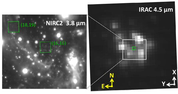
All observations in this Spitzer Space Telescope program (ID#10060) used IRAC in subarray mode, which obtains 64 consecutive images (a “frame set”) of a 32$\times$32 pixel region (1$\farcs$21 per pixel) near the corner of the 256$\times$256 pixel array. The observations were conducted as three custom “Instrument Engineering Requests” (IERs) because the standard IRAC Astronomical Observation Template does not allow the observation sequence we designed for this program. We used the “PCRS Peakup” mode to position Sgr A* as close as possible to the center of pixel (16,16). The detailed design of the IERs is described in Appendix A.

For our data reduction we used the standard Basic Calibrated Data (BCD) products (version S19.1.0) downloaded from the Spitzer Heritage Archive. Because we expect no detectable variation from Sgr A* on a time scale of 6.4 s (based on extrapolations of the source characteristics observed in the $K$-band and the noise level of the IRAC observations at 4.5 µm), the first step in the reduction was to combine each frame set into a single 32$\times$32 pixel image or “6.4-s BCD coadd”. This was done using the subcoadd_bcd routine in the IRACproc image processing software (Schuster et al. 2006), which performs an average of the frames with outlier rejection to eliminate cosmic rays.

Figure 2.— Excess flux density for Sgr A* and for the reference pixel in mJy. Blue points show the flux density for each 6.4-s BCD coadd, and the red lines show a running average smoothed with a Gaussian kernel having a 3 minute FWHM. The upper line and blue crosses are for Sgr A*, and the lower line and blue Xs are for reference pixel (18,19) offset vertically by $-7$ mJy. The calibrated values plotted are the difference between the observed value of the pixel in the 6.4-s BCD coadds and the predicted value for the measured $(X,Y)$ offset of each coadd , as described in Appendix A. Pixel values have been corrected to total flux density by the position-dependent ratio of total flux density to central-pixel signal. The horizontal axis shows the time in minutes relative to the start time of the first monitoring 6.4s BCD coadd.

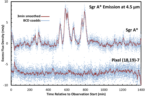
We extracted the flux density of Sgr A* for each BCD coadd as described in Appendix A. The resulting light curve is shown in the upper part of Figure 2. Because we have fit the signal in the relatively quiescent periods during the monitoring, we cannot derive the baseline flux from Sgr A* itself, only the excess above the level that persisted for a period shorter than the 23.4 hours that we monitored the source. Several significant peaks above the baseline level are seen, the largest $\sim$10 mJy. The rms variation of the 6.4-s BCD coadds for the time period 850–1400 minutes, which is relatively free of large peaks, is 0.9 mJy. There is also a deviation from the model fit in the first 100 minutes that appears different from the subsequent variations. This might indicate some systematic error in our fit at the beginning of the time series. We will be able to investigate this possible effect further after we obtain more monitoring observations scheduled for 2014 June–July.

Table 1Sgr A* Light Curve Data

Observation	Sgr A*	Reference
Date	Flux Density	Flux Density
(MJD)	(Jy)	(Jy)
56636.1808736	0.00210	0.00036
56636.1809705	0.00404	0.00228
56636.1810678	0.00393	0.00001
56636.1811650	0.00294	0.00021
56636.1812623	0.00233	0.00096
56636.1813596	0.00299	-0.00080
56636.1814566	0.00338	-0.00046
56636.1815536	0.00215	0.00025
56636.1816511	0.00276	-0.00028
56636.1817483	0.00239	-0.00058

As a test of our reduction method, we extracted the output of a reference pixel (18,19) in the same way as for (16,16), also shown in Figure 2. There is one peak in the extracted flux density for the reference pixel near the beginning of the time series that rises to $\sim$2.5 mJy in the smoothed data, but other fluctuations are smaller, and the rms variation is similar to that for Sgr A* pixel (16,16). The light curve data for Sgr A* and the reference pixel (18,19) are given in Table 1.

3. Variability properties of Sgr A* at 4.5 $\mu$m

The statistics of the Sgr A* NIR variability have been well characterized on the basis of a decade of 2.1–2.2 $\mu$m ($K$-band) observations with AO instruments at the VLT (Dodds-Eden et al., 2011; Witzel et al., 2012) and Keck (Do et al., 2009) observatories and with the two observatories combined (Meyer et al., 2009). The main properties are:

• The Sgr A* spectral index $\alpha$ ($f_{\nu}\propto\nu^{-\alpha}$) measured between 1.6 and 3.7 $\mu$m is $0.6\pm 0.2$, where the quoted uncertainty includes the uncertainty in the differential extinction and the possibility of small variations in $\alpha$ as $f_{\nu}$ varies. The spectral index variations have been observed to be uncorrelated with the flux density of the source, and they are small enough to be disregarded in our analysis (Hornstein et al. 2007 and references therein, Witzel et al. in prep.).

• The probability distribution of the intrinsic (reddening corrected) flux density $f_{K}$ at 2.2 $\mu$m is skewed, i.e. it shows a low median value ($\sim$1 mJy) and a tail toward high flux densities (flux densities as high as 30 mJy have been measured). The flux density distribution (FDD) can be described by a power law with index $\beta=4.22$ and a normalization $f_{0K}=3.57$ mJy (Witzel et al., 2012, eq. 9):

  $$\begin{split}P(f_{K})=[(\beta-1)/(f_{0K})][(f_{K}+f_{0K})/(f_{0K})]^{-\beta},\qquad f_{K}\geq 0\\ P(f_{K})=0,\qquad f_{K}<0.\end{split}$$ (1)

  The cutoff at zero flux density makes the power-law normalizable and guarantees that the intrinsic flux density of the source is never negative.

• The NIR variability shows a so-called rms–flux relation, i.e., the typical amplitude of variation is proportional to the flux density at which the variation occurs (Witzel et al. 2012). The variability is continuous and shows no indication of a quiescent state or different variability states (Witzel et al. 2012, Meyer et al. 2014).

• The PSD of the variability is a red-noise power-law spectrum with break at a temporal frequency $f_{bK}$ corresponding to a few hundred minutes:

  $$\begin{split}{\rm PSD}(f_{t})&\propto f_{t}^{-\gamma_{1}},\qquad f_{t}>f_{bK}\\ {\rm PSD}(f_{t})&\propto f_{bK}^{\gamma_{0}-\gamma_{1}}f_{t}^{-\gamma_{0}},\qquad f_{t}\leq f_{bK}\end{split}$$ (2)

  The value of $f_{bK}$ corresponds to $154^{+124}_{-87}$ minutes according to Meyer et al. (2009) or to 100–1000 minutes according to Witzel et al. (2012). The power-law index for long time intervals is $\gamma_{0}\approx 0$ and for short time intervals is $\gamma_{1}\approx 2.0$ . Witzel et al. (2012) also tested PSD models with a second break according to equation (2) and the additional equation:

  $${\rm PSD}(f_{t})\propto f_{bK,2}^{\gamma_{2}-\gamma_{1}}f_{t}^{-\gamma_{2}},\qquad f_{t}\leq f_{bK,2}\;\;,$$ (3)

  and $f_{bK,2}=0.05$, which resulted in higher acceptance values but not in a significant improvement that justified the additional parameters.

The goal of our statistical analysis is to investigate whether the 4.5 $\mu$m light curve can be understood with the existing models for the FDD and the PSD. We applied methods similar to those of Witzel et al. but modified them to account for:

• higher measurement noise and different baseline flux density level owing to unresolved nearby sources and the data reduction method

• having a single 23h sample during which the light curve maintains significant correlation from beginning to end. (The ground-based observation periods were shorter individually, and were separated by months or years and therefore have no correlation from one monitoring campaign to another.)

We analyzed the data in two steps, first looking at the FDD and second at the timing properties of the Spitzer data. Both steps made use of equation (28) of Witzel et al. (2012), which allows us to transform a unit normal-distributed random variable $y$ into a power-law distributed random variable $T(y)$ that takes on values $0<T(y)<\infty$:

$$T(y)=f_{\rm{0}}\cdot\left\{\frac{1}{2}\left[1+{\rm{erf}}\left(\frac{y}{\sqrt{2}}\right)\right]\right\}^{\frac{1}{\left(1-\beta\right)}}-f_{\rm{0}}~{}~{}.$$ (4)

where erf is the Gaussian error function, the power-law index $\beta=4.22$, and $f_{0}$ is the normalization flux density at the wavelength observed.

3.1. Flux density distribution

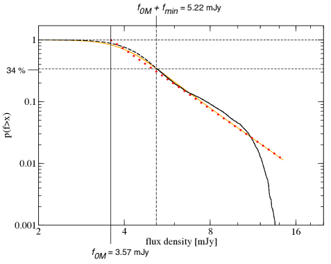
Even an observation duration of $\sim$23 h may not be vastly longer than the coherence timescale, and its FDD is only a single sample of the distribution of the variability process. As a consequence, the estimate of the FDD power-law index $\beta$ is uncertain even if the data are known to be drawn from a power-law distribution. Therefore, instead of deriving the power-law parameters independently from our dataset, we have adopted the parameters measured in the $K$-band (Witzel et al., 2012) and determined whether the new dataset is a likely realization of the same random process. The metric of comparison is the Kolmogorov-Smirnov ($KS$) statistic, for which we derived acceptance levels after establishing the timing properties by Monte Carlo simulations as described in Section 3.2.

We determined the $KS$ value in the following way:

• Due to the measurement techniques described above in §2, the empirically measured 4.5 µm flux densities $f$ omit a component corresponding to the average flux density when Sgr A* is in its relatively quiescent periods. This extra component is represented by a constant $c$, and we calculated the empirical complementary (i.e., $P(f>x)$ rather than $P(f<x)$) cumulative distribution function ${\rm CDF}(f+c)$ from the observed light curve.

• For comparison with the measured light curve, we generated $10^{7}$ unit normal-distributed random numbers and transformed them into power-law distributed numbers according to equation (4). The resulting values were then multiplied by a factor $s$ (to scale the dereddened $K$-band flux density values to the observed 4.5 µm flux density) to represent simulated values of $(f+c)$ at 4.5 µm. To these we added Gaussian white noise with a standard deviation $\sigma=0.7$ mJy. This value, rather than the empirical standard deviation $\sigma=0.9$ mJy, is justified by the low-time-lag value of the structure function derived in the next section and is consistent with intrinsic fluctuations of Sgr A* of $\sim$0.6 mJy rms at the noise dominated flux levels. The result is simulated values of $f$ with the constant $c$ added, i.e, ($f+c$).

• From the simulated light curve, we calculated the complementary cumulative distribution function ${\rm{CDF}_{\rm{sim}}}({f+c})$ and resampled based on a linear interpolation to ensure the CDF flux densities are the same for all CDFs. Then we calculated

  $$KS=\max_{f>f_{\rm{min}}}\left[CDF(f+c)-CDF_{\rm{sim}}({f+c})\right]$$ (5)

  where the parameter $f_{\rm{min}}$ separates the part of the CDF that is noise dominated from the part actually represented by a power law.

The final calculation consisted of minimizing the $KS$ value over the parameters $c$, $s$, and $f_{\rm{min}}$. The result is shown in Figure 3. The best parameters are $c=0.94$ mJy, $s=1.0$, and $f_{\rm{min}}=1.65$ mJy, and the resulting best $KS$ value is $0.0133$ corresponding to a 1.3% maximum difference between the real CDF and the one generated from the best-fit model. The corresponding probability cannot be looked up in standard tables because the data are correlated but can be derived from simulations as discussed in Section 3.2.

Figure 3.— Complementary cumulative distribution function and power-law fit to the data. The CDF of the light curve data $f$ is shown in black. The solid part of the line represents flux densities that were used for the $KS$-value estimation, and the dashed black line is the part dominated by measurement noise. The simulated CDF for the best parameters is in orange, and the red squares show the power-law model adopted from pre-existing $K$-band data (Witzel et al., 2012). The plot abscissa is $f+f_{0M}$ (with $f_{0M}=s\cdot f_{0K}$) in order to show the noise-dominated region of the data and to make the power law display as a straight line. The vertical lines show the power law normalization $f_{0M}$ (3.57 mJy) and the flux density ($f_{0M}+f_{min}=5.22\mu$Jy) at which the simulated CDF (orange) begins to deviate from the power law (red) due to measurement noise.

Table 2PSD models and their probabilities

	PSD 1	PSD 2	PSD 3	PSD 4
$f_{bK}$	0.0065 $\rm{min}^{-1}$	0.0065 $\rm{min}^{-1}$	0.0018 $\rm{min}^{-1}$	0.0018 $\rm{min}^{-1}$
$f_{bK,2}$	$\cdots$	0.05 $\rm{min}^{-1}$	$\cdots$	0.05 $\rm{min}^{-1}$
$\gamma_{1}$	2.0	2.0	2.0	2.0
$\gamma_{2}$	$\cdots$	3.8	$\cdots$	3.8
$p(\rm{CDF})$	0.1110	0.2032	0.1697	0.1750
$p(\chi^{2}|\rm{CDF})$	0.0032	0.0261	0.0488	0.1033
$p(\chi^{2}|\rm{CDF})\cdot p(\rm{CDF})$	0.00036	0.00530	0.00828	0.01807
freq.	1/2814	1/189	1/121	1/55
$p(\chi^{2}_{\rm{ps}})$	0.41	0.44	0.74	0.73

Figure 4.— Structure function of the light curve of Sgr A* (black) and of the comparison pixel (red). The vertical line at 702 minutes marks half of the observing window duration. See §3.2 for more details.

Figure 5.— Real and simulated light curves. The upper right panel shows the observed data, and other panels show simulated light curves based on the best FDD model and a PSD-model with a break timescale at 154 minutes (model 1 in Table 2).

3.2. Timing analysis

Timing analysis is about understanding the statistics of flux density differences between measurement points separated by a given time interval. A natural metric for characterizing timing properties is the first-order structure function, which measures the mean value of the flux density variance for a given time lag $\tau$. It is defined as (Simonetti et al. 1985; Do et al. 2009):

$$V(\tau)=\langle\left[f\left(t+\tau\right)-f(t)\right]^{2}\rangle~{}~{}.$$ (6)

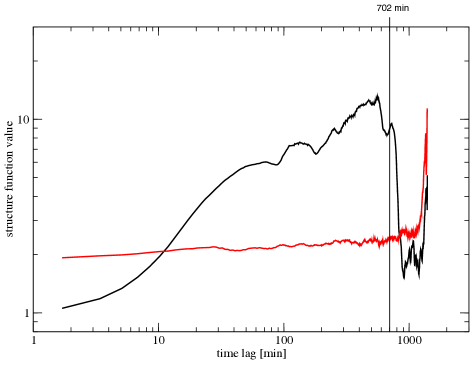
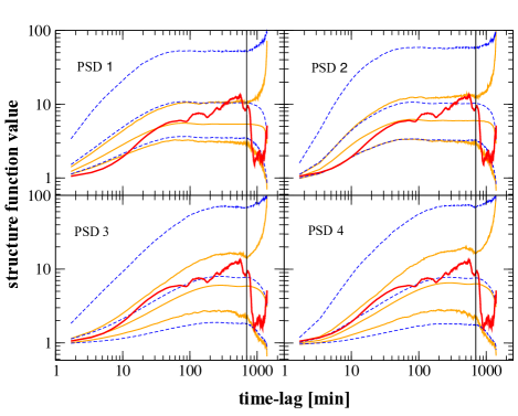
The structure function is the suitable metric in the case of data with unequal sampling, large gaps, or an observation window not vastly larger than the coherence timescale, which are sampling properties that introduce biases to standard Fourier techniques. The ultimate goal is to determine the shape of the PSD of the underlying process. Computing the PSD from a given structure function is not a trivial task. Only for very idealized cases can an analytical expression be used (Simonetti et al., 1985; Emmanoulopoulos et al., 2010). In general, Monte Carlo simulations that use the appropriate window function have to be used. The method applied here derives structure functions for a given PSD in a Monte Carlo simulation and determines the probability of the observed structure function and is very similar to the methods described by Uttley et al. (2002), Do et al. (2009), and Meyer et al. (2009). The observed structure function of our 4.5 µm light curve is shown in Figure 4 with a time-lag binning of 1.7 minutes. While the values for Sgr A* cover more than one order of magnitude, the structure function of the comparison pixel is almost constant, showing that the measurement noise is close to white.

The observed light curve (Figure 2) has its brightest peaks occurring close to the middle of the light curve with long, almost featureless stretches on both sides. This is reflected in the structure function by a maximum near 700 minutes followed by a steep decline at longer time lags. However, time lags larger than half the $\sim$1400 minute light curve duration have large uncertainties because progressively fewer flux density points contribute to the structure function. (For shorter time lags, all the flux density points in the light curve contribute to every structure function value though in different combinations. The limit is that only two light curve points contribute to the structure function at the full light curve duration.)

Figure 6.— Real and simulated light curves. The upper right panel shows the observed data, and other panels show simulated light curves based on the best FDD-model and a PSD model with a break timescale at 560 minutes (model 4 in Table 2).

The formal way to infer best-fit parameters of the PSD (including uncertainties) from our data would be to use the likelihood function $p(\chi^{2}|\rm{CDF})$ to derive the PSD parameters (slopes, break timescales, and their errors) by maximizing the likelihood function. Due to the high computational demands of the simulation process described in Appendix B and with only one 23.4h dataset, our goal here is to illustrate the advantages of such long, continuous monitoring rather than to explore the full parameter space. We therefore developed a pseudo $\chi^{2}$ ($\chi^{2}_{\rm{ps}}$) metric to quantify the difference between structure functions, and the likelihood functions $p(\chi^{2})$ and $p(\chi^{2}|\rm{CDF})$. The result quantifies the relative probability of individual PSD models, as described in detail in Appendix B. We restricted our analysis to four selected PSD models (listed in Table 2), which represent the following scenarios discussed in the literature: 1) a timescale of 154 minutes (Meyer et al., 2009; Dexter et al., 2014); 2) same as model 1 but with an additional timescale in the range of the debated quasi-periodic oscillation (20 minutes; Genzel et al., 2003); 3) a timescale of 556 minutes, significantly larger than expected for orbital timescales but comparable to the timescale found in the sub-mm (Dexter et al., 2014) and indicated by the analysis of Witzel et al. (2012); and 4) same as model 3 but with the 20 minute timescale added.

The results of our simulations are given in Table 2. For the single-break PSD model 1, $10\%$ of the simulated light curves have an FDD in accordance with our constraints, and $0.4\%$ of these accepted light curves show modified $\chi^{2}$ values of the magnitude of the observed structure function. This means that one in about 2800 light curves has the observed FDD and structure function (or one 23h stretch every 7.8 years). In addition, this model does not explain the maximum of the structure function at a time lag of about 560 minutes. In contrast, the double-break PSD model 4 (with breaks at 20 and 560 minutes) produces $18\%$ of the simulated light curves having an FDD in accordance with our constraints. Fully $10\%$ of these show $\chi^{2}_{\rm{ps}}$ values of the magnitude of the observed structure function. This means that about one in 55 light curves has the observed FDD and structure function (or one 23h stretch every 8 weeks). Model 4 also produces confidence intervals that enclose the observed structure function for all time lags.

PSD models 2 and 3 reach comparable probabilities as PSF model 4. In particular, PSD model 2 (with a timescale of 154 min) shows a significantly improved likelihood with respect to model 1, but incorporates one additional parameter, the second break.

Using PSD model 4, we determined the acceptance value for the FDD by simulating 1000 23 h stretches and fitting their CDFs in the same way as described in section 3.1. By comparing the resulting $KS$ values to the one derived from our observations, we found a $p$-value of $65\%$, i.e., more than half of the realizations show higher $KS$-values than the measured light curve.

Figure 7.— Autocorrelation functions of real and simulated data. The green line shows the autocorrelation function of the observed data, and the blue line shows that of the simulated light curve in the upper left panel of Figure 6. The red line shows the autocorrelation function corresponding to PSD model 4 derived from a 20000 minute Gaussian light curve with 0.1 minute sampling, and the black line is the analogous autocorrelation function derived from a power law distributed light curve. The vertical black line marks the 556 minute break, and the horizontal black line marks the 1/e level, which is sometimes used as an alternative characteristic value to describe the timing behavior (also referred to as the timescale).

4. Discussion and Future Prospects

The statistical analysis shows that the data taken with Spitzer at 4.5 $\mu$m are fully consistent with the $K$-band light curves. The offset $c=0.94$ mJy is a plausible value for restoring the average Sgr A* flux density that was lost by our reduction method. The scaling factor $s=1.0$ suggests that the observed flux density at 4.5 $\mu$m is a good estimator of the dereddened flux density at 2.2 $\mu$m. The derivation of $s$ was based on the observed fluctuation amplitudes and is independent of prior knowledge of the source spectral index $\alpha=0.6$ derived from synchronous measurements in the range of 1.6 $\mu$m to 3.7 $\mu$m and the 4.5 $\mu$m extinction $A_{M}=1.0\pm 0.3$ mag (Schödel et al. 2011). These earlier observations predict $s=0.6^{+0.5}_{-0.3}$, and our value $s=1.0$ lies within the bright end of the $1\sigma$ range. This implies that the spectral properties previously found, in particular a spectral index $\alpha=0.6$ characteristic of optically thin synchrotron radiation, are valid for the extended range of 1.6 $\mu$m to 4.5 $\mu$m and that the flux density calibration worked consistently in both bands.

With the scaling factor known, we can characterize the sensitivity of the Spitzer measurements for the intrinsic variability of Sgr A*. The typical noise level of observations with VLT/NACO is $0.32$ mJy in the dereddened light curves with a cadence of about 1.2 minutes (Witzel et al. 2012) . The noise level in the 8.4-s cadence 4.5 µm BCD coadds before dereddening is about 0.7 mJy. If we block-average the BCD coadds over 7 points to create a cadence of about one minute, the $S/N$ of the Spitzer data is 0.25 mJy, a factor of $\sim$1.3 better than the average ground-based AO observations with VLT/NACO.

The timing analysis shows that the observed 4.5 µm light curve is consistent with the existing model for the FDD and PSD as derived from $K$-band measurements. Based on the flux density distribution measured with the VLT, the 23 h Spitzer light curve helps discriminate between proposed models for the PSD beyond what could be achieved by continued ground based observations only: in the analysis of Witzel et al. (2012), the likelihood ratio between a timescale of 154 minutes and PSD slope of 2.0 ($p(\chi^{2})=75\%$) and the model with the highest likelihood (break at 588 minutes, $p(\chi^{2})>94\%$) is 1.25. In our analysis, the likelihood ratio between PSD 1 ($p(\chi^{2})=41\%$) and PSD 4 ($p(\chi^{2})=74\%$) is 1.8. The continuity of the sampling allowed us to develop a metric that is even more sensitive, the FDD-constrained likelihood $p(\chi^{2}|\rm{CDF})$, in which PSD 1 is estimated to be 51 times less likely than PSD 4. Under these FDD constraints, the observed structure function maximum values between the time lags of 400 minutes and 600 minutes are beyond the $99.7\%$-confidence levels of structure functions generated with PSD 1.

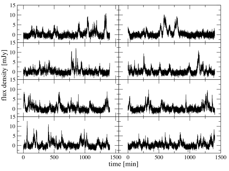
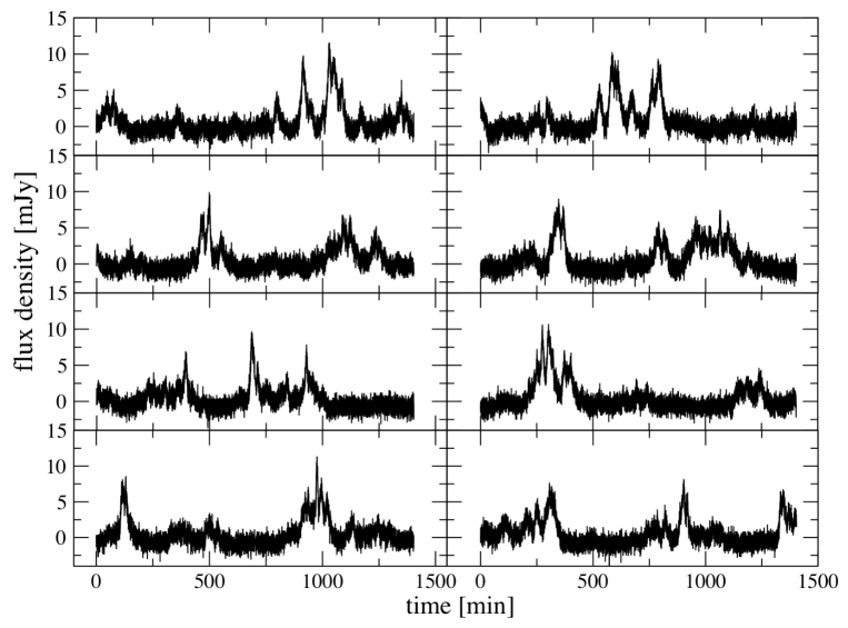
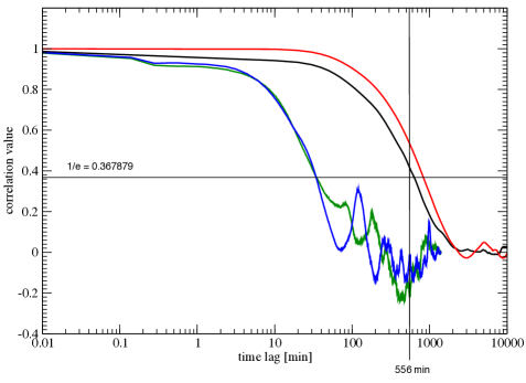
The correlation timescale influences the length of the gaps between flux outbursts and the width of the flux peaks. A longer timescale means longer gaps and wider peaks, a shorter timescale means shorter gaps and narrower peaks. To further illustrate differences between various PSDs, Figures 5 and 6 show example light curves created with PSD models 1 and 4. The model with the lower timescale shows many smaller outbursts but fails to reproduce long stretches of flux densities very close to the baseline. The model with the longer break timescale matches the visual impression of the observed data, showing rare large excursions clustered in time. Light curves covering only $10-20\%$ of a day are not sensitive to this difference. Figure 7 shows the autocorrelation function of the data in comparison to simulated 24 hour light curves, and model 4 gives an excellent fit in this metric as well.

The analysis here is not yet able to rule out break timescales as short as 154 minutes due to the strong correlation between slopes and break timescales. PSD 2 (154 minute break combined with a steeper slope of 3.8 for timescales shorter than a second break at 20 minutes) is only 3.4 times less likely than PSD 4 and satisfies the $99.7\%$-confidence levels for all time lags $\leq$ 700 minutes. However, additional continuous $\sim$23 h monitoring will contribute essential information. Future observations of Sgr A* with Spitzer/IRAC are planned for 2014 June–July (three epochs) and November–December (two epochs). These will allow independent verification of the FDD model and a rigorous determination of the break time scale and its uncertainty based on simultaneous Bayesian fitting of the CDF and structure function. They should also show whether a second break (at 20 minutes) in the PSD is warranted.

The variability of Sgr A* as a measure of the response of its accretion flow to G2 is one of the key observables that can elucidate the physics close to the event horizon. The latest orbital estimates put G2’s time of closest approach around 2014 March ($2014.21\pm 0.13$; Meyer et al. 2013; Phifer et al. 2013; Gillessen et al. 2013b), which is just when the Galactic center becomes observable again from ground-based telescopes (from roughly October to February the Sun does not permit Sgr A* observations in the IR from Earth). The light curve reported here therefore fills a crucial gap; these were the only IR observations possible in 2013 December, just before G2’s closest approach. Our analysis shows that G2 had not yet had a measurable impact on Sgr A*: the statistical properties are exactly as expected from more than a decade of $K$-band observations (Witzel et al. 2012, Meyer et al. 2014). Our observations this year should show whether and how Sgr A* reacts to the presence of G2.

Figure 8.— Top panel: $(X,Y)$ offsets in pixels for the two monitoring observations. The purple line shows the $X$ position and the green line the $Y$ position of Sgr A* relative to the center of pixel (16,16). The break near the center of the plot is where the peakup operation occurred between the first and second monitoring IERs. Bottom panel: Value of pixel (16,16) in the 6.4-s BCD coadds, in units of MJy sr^-1. The blue line shows the data, and the red line is the polynomial model fit described in the text (equation 7). The horizontal axis shows the time in minutes relative to the start time of the first monitoring BCD. The panels have the same horizontal scale.

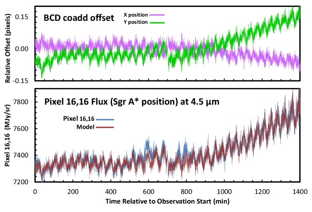
After constructing the 6.4-s BCD coadds as described in §2, the next reduction step was to derive their accurate relative positions. We used the xregister routine in IRAF to perform a cross-correlation between image pairs to determine the relative offset. In order to accurately register the subarray frames and correct the World Coordinate System (WCS) defined in the FITS headers of each BCD, we first performed a cross-correlation between the first 0.1 s BCD coadd and each of the mapping IER BCD coadds to determine the relative offsets, and wrote the relative RA and Dec into the BCD coadd headers. We then used IRACproc to construct a mosaic using these frames at a resolution of 0$\farcs$6 pixel^-1. The RA and Dec of this mosaic were then determined by comparison to a ground-based L-band adaptive optics image obtained with NIRC2 at Keck (see Figure 1). The 4.5 $\mu$m IRAC mosaic was then re-projected back to the instrumental pixel scale with Sgr A* placed at the center of pixel (16,16). The reprojected mosaic was then used as a reference image, and the relative offset of each of the monitoring BCD coadds was determined by cross-correlation with this reference image. The derived relative offsets for the monitoring BCD coadds are shown in the top panel of Figure 8. The Spitzer spacecraft battery-heater-related pointing oscillation (Grillmair et al. 2012) is visible throughout the observation. It has a period of $\sim$40 minutes and a peak-to-peak amplitude of $\sim$0.05 pixels in X and Y. The mean pointing was relatively constant during the first monitoring IER, but during the second there was a roughly constant drift throughout the observation, resulting in an offset of $-0.10$ pixel in X and +0.25 pixels in Y by the end of the 700 minute IER.

Because the intrinsic IRAC response is extremely stable, the pixel output depends only on the position of the frame on the sky and the variability of Sgr A*. This is similar but not identical to the case of exoplanet transit observations, where pointing variations cause a single point source to move relative to the pixel center (e.g., Ballard et al. 2010; Ballard et al. 2014). In the exoplanet case, a single bright point source dominates and the pointing variations cause changes in the measured signal as result of the structure of the IRAC intra-pixel response, which requires a multiplicative correction. In the Galactic center case, the major correction is additive because the pointing-induced signal variations are due to the IRAC pixel sampling different parts of the complex background of unresolved sources and extended emission near Sgr A*.

The bottom panel in Figure 8 shows the effect of the pointing variations on the pixel output of the coadded BCD frame sets. In addition to the position-dependent variations, the output includes the noise inherent in the observation and the variability of Sgr A* itself. The median surface brightness is 7385 MJy sr^-1 (or 257 mJy pixel^-1), and the maximum surface brightness gradient is 1600 MJy sr^-1 arcsec^-1 (56 mJy pixel^-1 arcsec^-1 ).

We experimented with several methods for extracting the Sgr A* flux density, including simple aperture photometry, difference imaging plus aperture photometry, and using various linear combinations of the eight pixels adjacent to (16,16) to adjust the flux density. No method gave lower noise during the low parts of the light curve than simply using pixel (16,16) alone, corrected as described below. Some of the other methods resulted in large artifacts (many times the level of the signal) that were strongly correlated to the frame position, clearly failing to remove the effects of the pointing variations. From standard star measurements we know that $\sim$40% of the flux from a well-centered point source will fall within the central pixel, and less than 10% will fall in the next brightest neighboring pixel. The pixels near Sgr A* sample the complex field of bright, unresolved point sources and significant extended emission in the Galactic center region, so they all vary strongly as a function of position. Therefore, adding neighboring pixels to the analysis contributes more systematic errors than additional signal and does not improve the signal to noise of the measurement.

To model the dependence of the pixel output on the X,Y position of Sgr A* in the frame, we used a second-degree polynomial

$$F(X,Y)=a+bX+cY+dXY+eX^{2}+fY^{2}$$ (7)

and determined the coefficients by performing a least-squares fit to minimize the residuals between the function and the monitoring data. The first iteration showed that there were time intervals where the data deviated significantly from the fit; these regions were then excluded from the fit and the coefficients determined again. The final fitted values of the coefficients are $a=7379.8$, $b=1196.8$, $c=-1096.5$, $d=-197.2$, $e=-1948.4$, and $f=4704.6$. The model value is plotted at each of the positions observed along with the pixel (16,16) output in the bottom panel of Figure 8.

The initial measure of the variable component of the flux density from Sgr A* is the residual between the pixel (16,16) data value and the expected value determined by equation (7). These values have to be multiplied by the position-dependent ratio of total flux density to central pixel signal for a point source in order to determine the total variable component of the flux from Sgr A*. The flux from a point source is distributed across IRAC pixels according to the pixel response function (PRF). The IRAC calibration was determined using aperture photometry of stars (Reach et al. 2005), so we used existing observations of a standard star (BD+$67\arcdeg$ 1044) taken in subarray mode with 0.1 s frame times to determine the relationship between central pixel flux and centroid position of a point source, relative to the total source flux. We used $\sim$18,800 warm mission subarray measurements originally taken to map out the subarray response for exoplanet observations. Standard star data with centroids ranging from $-0.1$ to $+$0.2 in $X$ and $-0.2$ to $+$0.2 in $Y$ (relative to the center of pixel 16,16) were used to cover the range of pixel coordinates seen in the Sgr A* data. A fourth-degree polynomial as a function of $X,Y$ position was needed to fit the central pixel to total flux ratio. This polynomial reproduces the measurements to an accuracy of 0.04% rms. The central value of the fitted function is 0.407, and other values range from 0.335 to 0.430 over the observed range of Sgr A* positions. The final calibrated light curve data are given in Table 1, and plotted in Figure 2.

As a test of our reduction method, we also extracted and modeled the output of pixel (18,19) in the same way as for (16,16). This pixel is on an image location with a significant gradient and not on a local maximum, similar to pixel (16,16) but far enough away from it that it will not see the variability from Sgr A* (see Figure 1). The median value in this pixel is ${\sim}10^{4}$ MJy sr^-1 (350 mJy pixel^-1). The fit coefficients as in eq. 7 for pixel (18,19) are $a=10064.6$, $b=6686.8$, $c=-4260.6$, $d=5658.8$, $e=-4263.9$, and $f=-761.7$. The results are plotted in Figure 2. There is one peak near the beginning of the time series that rises to $\sim$2.5 mJy in the smoothed data, but other fluctuations are smaller, and the rms is similar to that for pixel (16,16). The reference pixel data are also given in Table 1, and plotted in Figure 2.

APPENDIX B

STATISTICAL ANALYSIS METHODS FOR THE POWER SPECTRAL DENSITY

Predicted structure functions offer a way to test PSD models. For each proposed PSD, we derived a set of structure functions from simulated light curves. We used the algorithm from Witzel et al. (2012) based on the method by Timmer & Koenig (1995) to create light curves that exhibit the power-law FDD described in Section 3.1. The procedure began by drawing Fourier coefficients for each frequency from a Gaussian distribution with a variance proportional to the value of the PSD at that frequency. The resulting PSD was Fourier-transformed to the time domain and normalized to unity variance. At this stage, the equally spaced data were optionally resampled to the cadence of the observed light curve. With or without resampling, each point was transformed according to equation (4). Finally, an independent Gaussian noise was added to each point to account for measurement errors. For all models tested here, the best result for the first time lag was achieved by giving the white noise a standard deviation of 0.7 mJy.

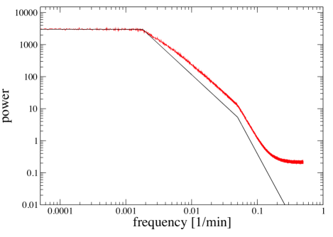
The important property of the algorithm for generating predicted structure functions is the normalization step. It ensures that for any break timescale and PSD slope, the PSD is normalized in a way that flux densities occur with the observed probabilities. In particular, it enables us to compare the absolute values of the structure function of simulated light curves with the observed structure function. The transformation changes the PSD of the generated light curve slightly (see difference between input PSD and effective PSD in Figure 9 illustrated for a double broken PSD). The break timescales, however, are not affected.

Figure 9.— PSD versus temporal frequency for model 4 (Table 2). The black line shows the input PSD that creates the Gaussian time series. The red line shows the PSD derived from 10000 simulated light curves with a length of 20000 minutes each, sampled at 0.1 minute intervals. The difference between the two lines arises because the initial light curve created from the PSD is Gaussian, but the source fluctuations are modeled as a power law distribution. The flattening towards highest frequencies is caused by the white measurement noise. The break locations are the same for both distributions, and are given in Table 2.

For each of the PSD models, we generated 10000 light curves with a sampling of 0.1 minutes and a length of 20000 minutes (see Figure 10), resampled a 23 h middle section (avoiding the ends in order to avoid red-noise leakage) to the actual cadence of the light curve, and calculated structure functions and the most probable structure function value for each time lag $\tau_{m}$:

$$\tilde{V}(\tau_{m})=\exp{\langle\ln[V(\tau_{m})]\rangle}~{}~{},$$ (8)

and its $95\%$- and $99.7\%$-confidence levels (by determining the 0.135^th, 2.275^th, 97.725^th, and 99.865^th percentile). We also calculated the pseudo-$\chi^{2}$ (Emmanoulopoulos et al. 2010):

$$\chi^{2}_{\rm{ps}}=\sum_{m}\left(\frac{\langle\ln[V(\tau_{m})]\rangle-\ln[V(\tau_{m})]}{\sigma_{m}}\right)^{2}~{}~{},$$ (9)

with $\sigma_{m}$ the variance of $\ln[V(\tau_{m})]$. Pseudo-$\chi^{2}$ quantifies the deviation from the most probable values, $\tilde{V}(\tau_{m})$, summed over all time lags and defines a likelihood function for the PSD parameter set by determining the fraction of simulated structure functions with a worse $\chi^{2}_{\rm{ps}}$ than the observed data. The results for the four PSD models are shown in Figure 10.

For every tested PSD model, the $95\%$-confidence level is wide enough to account for the deviations of the observed structure function from the most probable values up to a time lag of 700 minutes. The longer-timescale PSD models have likelihood values of $p(\chi^{2}_{\rm{ps}})=73\%$ and $p(\chi^{2}_{\rm{ps}})=74\%$, whereas the 154 minute PSDs have likelihood values of $p(\chi^{2}_{\rm{ps}})=41\%$ and $p(\chi^{2}_{\rm{ps}})=44\%$. However, testing the structure functions against the general set of 23 h stretches generated from a particular PSD does not take advantage of all the information. The amplitude of typical flux density fluctuations scales with the flux density level itself (rms-flux relation). Thus, letting light curves that exhibit very different FDDs over 23 h contribute to the statistics of the structure function is not acknowledging that the measured FDD has a specific flux density maximum.

Figure 10.— The structure function and confidence intervals for our four PSD models. The thick red lines show the observed data. The dashed blue lines show the most probable structure function values and their 95% confidence intervals for light curves without constraints. The orange solid lines represent the most probable structure function values and their 99.7% confidence intervals for light curves with matching CDFs (for all models the CDFs differ from the observed data by $<0.07$ and the peak flux density over 23.4 h differing by $<2.5$ mJy). The vertical lines mark the time lag corresponding to half the monitoring duration.

To take full advantage of the data, we defined a modified likelihood function based on a restricted set of light curves that have a maximum similar to that seen in the data (10.3$\pm 2.5$ mJy) and a similar CDF (maximum difference between observed and simulated CDF $<$0.07). This likelihood function was defined as the product of the probability $p(\rm{CDF})$ to find the observed FDD and the probability to find a structure function with a larger $\chi^{2}_{\rm{ps}}$ value, $p(\chi^{2}_{\rm{ps}}|\rm{CDF})$.

Additionally, the constraints on the FDD allow us to determine whether the measured structure function values are in the range of the statistical expectation for the observed flux densities. Introducing flux density constraints makes sense only for continuous datasets without gaps larger than the time lag binning. Otherwise, depending on the observation gaps, the FDD from which the individual time lag draws changes, and the constraints do not affect each time lag equally. The $\chi^{2}_{\rm{ps}}$ value in this case has to be computed from time lags $\leq 700$ minutes only (which draw from the full number of data points in the light curve), and the confidence intervals derived in this way are strictly correct only for those shorter time lags (the FDD of flux densities contributing to structure function values at higher time lags would have to be separately matched with the simulation, time lag by time lag, requiring excessive computation time).

References

- Abarca et al. (2014) Abarca, D., Sa̧dowski, A., & Sironi, L. 2014, MNRAS, 440, 1125
- Anninos et al. (2012) Anninos, P., Fragile, P. C., Wilson, J., & Murray, S. D. 2012, ApJ, 759, 132
- Arendt et al. (2008) Arendt, R. G., Gezari, D. Y., Stolovy, S. R., et al. 2008, ApJ, 685, 958
- Ballard et al. (2010) Ballard, S., Charbonneau, D., Deming, D., et al. 2010, PASP, 122, 1341
- Ballard et al. (2014) Ballard, S., Chaplin, W. J., Charbonneau, D., et al. 2014, ArXiv e-prints, arXiv:1405.3659
- Ballone et al. (2013) Ballone, A., Schartmann, M., Burkert, A., et al. 2013, ApJ, 776, 13
- Burkert et al. (2012) Burkert, A., Schartmann, M., Alig, C., et al. 2012, ApJ, 750, 58
- Clénet et al. (2004) Clénet, Y., Rouan, D., Gendron, E., et al. 2004, A&A, 417, L15
- Close et al. (1995) Close, L. M., McCarthy, Jr., D. W., & Melia, F. 1995, ApJ, 439, 682
- Dexter & Fragile (2013) Dexter, J., & Fragile, P. C. 2013, MNRAS, 432, 2252
- Dexter et al. (2014) Dexter, J., Kelly, B., Bower, G. C., et al. 2014, MNRAS, 442, 2797
- Dexter et al. (2013) —. 2013, ArXiv e-prints, arXiv:1308.5968
- Do et al. (2009) Do, T., Ghez, A. M., Morris, M. R., et al. 2009, ApJ, 691, 1021
- Dodds-Eden et al. (2011) Dodds-Eden, K., Gillessen, S., Fritz, T. K., et al. 2011, ApJ, 728, 37
- Eckart et al. (2006) Eckart, A., Schödel, R., Meyer, L., et al. 2006, A&A, 455, 1
- Eckart et al. (2004) Eckart, A., Baganoff, F. K., Morris, M., et al. 2004, A&A, 427, 1
- Eckart et al. (2008a) Eckart, A., Baganoff, F. K., Zamaninasab, M., et al. 2008a, A&A, 479, 625
- Eckart et al. (2008b) Eckart, A., Schödel, R., García-Marín, M., et al. 2008b, A&A, 492, 337
- Eckart et al. (2012) Eckart, A., García-Marín, M., Vogel, S. N., et al. 2012, A&A, 537, A52
- Eckart et al. (2013) Eckart, A., Mužić, K., Yazici, S., et al. 2013, A&A, 551, A18
- Emmanoulopoulos et al. (2010) Emmanoulopoulos, D., McHardy, I. M., & Uttley, P. 2010, MNRAS, 404, 931
- Fazio et al. (2004) Fazio, G. G., Hora, J. L., Allen, L. E., et al. 2004, ApJS, 154, 10
- Fragile et al. (2014) Fragile, P. C., Anninos, P., & Murray, S. D. 2014, ArXiv e-prints, arXiv:1401.0553
- Genzel et al. (1997) Genzel, R., Eckart, A., Ott, T., & Eisenhauer, F. 1997, MNRAS, 291, 219
- Genzel et al. (2003) Genzel, R., Schödel, R., Ott, T., et al. 2003, Nature, 425, 934
- Ghez et al. (2004) Ghez, A. M., Wright, S. A., Matthews, K., et al. 2004, ApJ, 601, L159
- Gillessen et al. (2012) Gillessen, S., Genzel, R., Fritz, T. K., et al. 2012, Nature, 481, 51
- Gillessen et al. (2013a) —. 2013a, ApJ, 763, 78
- Gillessen et al. (2013b) —. 2013b, ApJ, 774, 44
- Grillmair et al. (2012) Grillmair, C. J., Carey, S. J., Stauffer, J. R., et al. 2012, in Society of Photo-Optical Instrumentation Engineers (SPIE) Conference Series, Vol. 8448, Society of Photo-Optical Instrumentation Engineers (SPIE) Conference Series
- Hornstein et al. (2002) Hornstein, S. D., Ghez, A. M., Tanner, A., et al. 2002, ApJ, 577, L9
- Hornstein et al. (2007) Hornstein, S. D., Matthews, K., Ghez, A. M., et al. 2007, ApJ, 667, 900
- Ingalls et al. (2012) Ingalls, J. G., Krick, J. E., Carey, S. J., et al. 2012, in Society of Photo-Optical Instrumentation Engineers (SPIE) Conference Series, Vol. 8442, Society of Photo-Optical Instrumentation Engineers (SPIE) Conference Series
- Meyer et al. (2009) Meyer, L., Do, T., Ghez, A., et al. 2009, ApJ, 694, L87
- Meyer et al. (2014) Meyer, L., Witzel, G., Longstaff, F. A., & Ghez, A. M. 2014, ArXiv e-prints, arXiv:1403.5289
- Meyer et al. (2013) Meyer, L., Ghez, A. M., Witzel, G., et al. 2013, ArXiv e-prints, arXiv:1312.1715
- Miralda-Escudé (2012) Miralda-Escudé, J. 2012, ApJ, 756, 86
- Murray-Clay & Loeb (2012) Murray-Clay, R. A., & Loeb, A. 2012, Nature Communications, 3, arXiv:1112.4822
- Petrov et al. (2011) Petrov, L., Kovalev, Y. Y., Fomalont, E. B., & Gordon, D. 2011, AJ, 142, 35
- Phifer et al. (2013) Phifer, K., Do, T., Meyer, L., et al. 2013, ApJ, 773, L13
- Reach et al. (2005) Reach, W. T., Megeath, S. T., Cohen, M., et al. 2005, PASP, 117, 978
- Schartmann et al. (2012) Schartmann, M., Burkert, A., Alig, C., et al. 2012, ApJ, 755, 155
- Schödel et al. (2011) Schödel, R., Morris, M. R., Muzic, K., et al. 2011, A&A, 532, A83
- Schuster et al. (2006) Schuster, M. T., Marengo, M., & Patten, B. M. 2006, in Society of Photo-Optical Instrumentation Engineers (SPIE) Conference Series, Vol. 6270, Society of Photo-Optical Instrumentation Engineers (SPIE) Conference Series
- Scoville & Burkert (2013) Scoville, N., & Burkert, A. 2013, ApJ, 768, 108
- Shcherbakov (2013) Shcherbakov, R. V. 2013, ArXiv e-prints, arXiv:1311.4507
- Simonetti et al. (1985) Simonetti, J. H., Cordes, J. M., & Heeschen, D. S. 1985, ApJ, 296, 46
- Simons & Becklin (1996) Simons, D. A., & Becklin, E. E. 1996, AJ, 111, 1908
- Stolovy et al. (2006) Stolovy, S., Ramirez, S., Arendt, R. G., et al. 2006, Journal of Physics Conference Series, 54, 176
- Timmer & Koenig (1995) Timmer, J., & Koenig, M. 1995, A&A, 300, 707
- Tollestrup et al. (1989) Tollestrup, E. V., Becklin, E. E., & Capps, R. W. 1989, AJ, 98, 204
- Uttley et al. (2002) Uttley, P., McHardy, I. M., & Papadakis, I. E. 2002, MNRAS, 332, 231
- Viehmann et al. (2005) Viehmann, T., Eckart, A., Schödel, R., et al. 2005, A&A, 433, 117
- Werner et al. (2004) Werner, M. W., Roellig, T. L., Low, F. J., et al. 2004, ApJS, 154, 1
- Witzel et al. (2012) Witzel, G., Eckart, A., Bremer, M., et al. 2012, ApJS, 203, 18
- Yuan (2011) Yuan, F. 2011, ASP Conf. Ser., 439, 346
- Zamaninasab et al. (2008) Zamaninasab, M., Eckart, A., Meyer, L., et al. 2008, Journal of Physics Conference Series, 131, 012008