Source estimation with incoherent waves in random waveguides

Abstract

We study an inverse source problem for the acoustic wave equation in a random waveguide. The goal is to estimate the source of waves from measurements of the acoustic pressure at a remote array of sensors. The waveguide effect is due to boundaries that trap the waves and guide them in a preferred (range) direction, the waveguide axis, along which the medium is unbounded. The random waveguide is a model of perturbed ideal waveguides which have flat boundaries and are filled with known media that do not change with range. The perturbation consists of fluctuations of the boundary and of the wave speed due to numerous small inhomogeneities in the medium. The fluctuations are uncertain in applications, which is why we model them with random processes, and they cause significant cumulative scattering at long ranges from the source. The scattering effect manifests mathematically as an exponential decay of the expectation of the acoustic pressure, the coherent part of the wave. The incoherent wave is modeled by the random fluctuations of the acoustic pressure, which dominate the expectation at long ranges from the source. We use the existing theory of wave propagation in random waveguides to analyze the inverse problem of estimating the source from incoherent wave recordings at remote arrays. We show how to obtain from the incoherent measurements high fidelity estimates of the time resolved energy carried by the waveguide modes, and study the invertibility of the system of transport equations that model energy propagation in order to estimate the source.

1 Introduction

We study an inverse problem for the scalar (acoustic) wave equation, where we wish to estimate the source of waves from measurements of the acoustic pressure field $p(t,\vec{{\bf x}})$ at a remote array of receiver sensors. The waves propagate in a waveguide, meaning that they are trapped by boundaries and are guided in the range direction, the waveguide axis, along which the medium is unbounded. Ideally the boundaries are straight and the medium does not change with range. We consider perturbed waveguides filled with heterogeneous media, where the boundary and the wave speed have small fluctuations on scales similar to the wavelength. These fluctuations have little effect in the vicinity of the source, but they are important at long ranges because they cause significant cumulative wave scattering. We suppose that the array of receivers is far from the source, as is typical in applications in underwater acoustics, sound propagation in corrugated pipes, in tunnels, etc., and study how cumulative scattering impedes the inversion.

In most setups the fluctuations are uncertain, which is why we introduce a stochastic framework and model them with random processes. The inversion is carried in only one perturbed waveguide, meaning that the array measures one realization of the random pressure field, the solution of the wave equation in that waveguide. The stochastic framework allows us to study the chain of mappings from the uncertainty in the waveguide to the uncertainty of the array measurements and of the inversion results. The goal is to understand how to process the uncertain data and quantify what can be estimated about the source in a reliable (statistically stable) manner. Statistical stability means that the estimates do not change with the realization of the fluctuations of the waveguide, which are unknown.

The problem of imaging (localizing) sources in waveguides has been studied extensively in underwater acoustics [5, 21, 19, 1]. Typical imaging approaches are matched field and related coherent methods that match the measured $p(t,\vec{{\bf x}})$ with its mathematical model for search locations of the source. The model is based on wave propagation in ideal waveguides and the imaging is successful when $p(t,\vec{{\bf x}})$ is mostly coherent. The coherent part of $p(t,\vec{{\bf x}})$ is its statistical expectation ${\mathbb{E}}[p(t,\vec{{\bf x}})]$ with respect to realizations of the random waveguide, and the incoherent field is modeled by $p(t,\vec{{\bf x}})-{\mathbb{E}}[p(t,\vec{{\bf x}})]$. As the waves propagate in the random waveguide they lose coherence due to scattering by the fluctuations of the boundary and the inhomogeneities in the medium. This manifests as an exponential decay in range of the expectation ${\mathbb{E}}[p(t,\vec{{\bf x}})]$, and strengthening of the fluctuations $p(t,\vec{{\bf x}})-{\mathbb{E}}[p(t,\vec{{\bf x}})]$.

Detailed studies of the loss of coherence of sound waves due to cumulative scattering are given in [20, 10, 13, 18, 14] for waveguides filled with randomly heterogeneous media and in [4, 17] for waveguides with random boundaries. These waveguides are two dimensional models of the ocean, and they may leak (radiate) in the ocean floor. The problem is similar in three dimensional acoustic waveguides with bounded cross-section. We refer to [6] for wave propagation in three dimensional waveguide models of the ocean which have unbounded cross-section and random pressure release top boundary, and to [3, 22] for three dimensional electromagnetic random waveguides. In all cases the analysis of loss of coherence is based on the decomposition of the wave field in an infinite set of monochromatic waves called waveguide modes, which are special solutions of the wave equation in the ideal waveguide. Finitely many modes are propagating waves, and we may associate them with plane waves that strike the boundary at different angles of incidence and are reflected repeatedly. The remaining infinitely many modes are evanescent and/or radiating waves. The cumulative scattering in the waveguide is modeled by fluctuations of the amplitudes of the modes. When scattering is weak, as is the case at moderate distances from the source, the amplitudes are approximately constant in range, and they are determined solely by the source excitation. Scattering builds up over long ranges and the mode amplitudes become random fields with exponentially decaying expectation on range scales called scattering mean free paths.

The mode dependence of the scattering mean free paths is analyzed in [4]. It turns out that the slow modes, which correspond to plane waves that strike the boundary at almost normal incidence, are most affected by scattering. These waves have long trajectories from the source to the array, and thus interact more with the boundary and medium fluctuations. We refer to [7] for an adaptive coherent imaging approach which detects which modes are incoherent and filters them out from the measurements in order to achieve statistically stable results. See also the results in [21, 19, 25]. However, when the array is farther from the source than the scattering mean free paths of all the modes, the data is incoherent and coherent imaging methods like matched field cannot work. In this paper we assume that this is the case and study an inversion approach based on a system of transport equations that models the propagation of energy carried by the modes. This system is derived in [20, 13, 4] and is used in [8] to estimate the location of a point source in random waveguides. Here we study the inverse problem in more detail and answer the following questions: (1) How can we obtain reliable estimates of the mode energies from the incoherent pressure field measured at the array? (2) What kind of information about the source can we recover from the transport equations? (3) Can we quantify the deterioration of the inversion results in terms of the range offset between the source and the array?

We begin in section 2 with the mathematical formulation of the inverse problem, and recall in section 3 the model of the random wave field $p(t,\vec{{\bf x}})$ derived in [20, 13, 4, 9]. The main results of the paper are in sections 4 and 5. We motivate there the inversion based on energy transport, and describe the forward mapping from the source to the expectation of the time resolved energy carried by the modes. We show how to calculate this energy from the incoherent array data, and describe how to invert approximately the transport equations. The results quantify the limited information that can be recovered about the source. We end with a summary in section 6.

2 Formulation of the problem

Fig. 1: Schematic of the problem setup. The source emits a signal in a waveguide and the wave field is recorded at a remote array. The perturbed waveguide has fluctuating boundaries and is filled with a medium with fluctuating wave speed.

We limit our study to two dimensional waveguides with reflecting boundaries modeled by pressure release boundary conditions. This is for simplicity, but the results extend to other boundary conditions and to leaky and three dimensional waveguides, as discussed in section 6. We illustrate the setup in Figure 1, and introduce the system of coordinates $\vec{{\bf x}}=(x,z)$ with range $z$ originating from the center of the source. The waveguide occupies the domain

$$\Omega=\left\{\vec{{\bf x}}=(x,z):~{}~{}x\in(X_{{}_{B}}(z),X_{{}_{T}}(z)),~{}~{}z\in\mathbb{R}\right\},$$

where the cross-range $x$ takes values between the bottom and top boundaries modeled by $X_{{}_{B}}(z)$ and $X_{{}_{T}}(z)$. The source has an unknown density $\rho(\vec{{\bf x}})$ which is compactly supported in $\Omega$, near $z=0$, and emits a signal $F(t)$ which is a pulse $f(Bt)$ of support of order $1/B$ around $t=0$, modulated by an oscillatory exponential

$$F(t)=e^{-i\omega_{o}t}f(Bt).$$ (1)

We introduce the bandwidth $B$ in the argument of the pulse to emphasize that the Fourier transform $\widehat{F}(\omega)$ of the signal is supported in the interval $(\omega_{o}-\pi B,\omega_{o}+\pi B)$ around the central frequency $\omega_{o}$,

$$\widehat{F}(\omega)=\int_{-\infty}^{\infty}dt\,F(t)e^{i\omega t}=\frac{1}{B}\widehat{f}\left(\frac{\omega-\omega_{o}}{B}\right).$$ (2)

The array is a collection of receivers that are placed close together in the set

$${A}=\left\{\vec{{\bf x}}_{{}_{\mathcal{A}}}=(x,z_{{}_{\mathcal{A}}}):~{}~{}x\in\mathcal{A}\subset[X_{{}_{B}}(z),X_{{}_{T}}(z)]\right\},$$

at range $z_{{}_{\mathcal{A}}}>0$ from the source, where $\mathcal{A}$ is an interval called the array aperture. The receivers record the acoustic pressure field $p(t,\vec{{\bf x}})$ modeled by the solution of the acoustic wave equation

$$\left[\partial_{x}^{2}+\partial_{z}^{2}-c^{-2}(\vec{{\bf x}})\partial^{2}_{t}\right]p(t,\vec{{\bf x}})=F(t)\rho(\vec{{\bf x}}),\quad\vec{{\bf x}}\in\Omega,~{}~{}t>0,$$ (3)

with pressure release boundary conditions

$$p(t,\vec{{\bf x}})=0,\quad t>0,~{}~{}\vec{{\bf x}}\in\partial\Omega=\left\{\vec{{\bf x}}=(x,z):~{}~{}x\in\{X_{{}_{B}}(z),X_{{}_{T}}(z)\},~{}~{}z\in\mathbb{R}\right\},$$ (4)

and initial condition $p(t,\vec{{\bf x}})\equiv 0$ for $t\ll 0$. Here $c(\vec{{\bf x}})$ is the sound speed.

The inverse problem is to determine the source density $\rho(\vec{{\bf x}})$ from the array data recordings $D(t,x)$. We model them by

$$D(t,x)=p(t,\vec{{\bf x}}_{{}_{\mathcal{A}}})1_{{}_{\mathcal{A}}}(x)\chi\left(\frac{t-t_{o}}{\mathcal{T}}\right),\quad\vec{{\bf x}}_{{}_{\mathcal{A}}}=(x,z_{{}_{\mathcal{A}}}),$$ (5)

using a recording time window $\chi$ centered at $t_{o}$ and of duration $\mathcal{T}$. We can take any continuous, compactly supported $\chi$, but we assume henceforth that it equals one in the interval $(-1/2,1/2)$ and tapers quickly to zero outside. We also approximate the array by a continuum aperture in the interval $\mathcal{A}$, and use the indicator function $1_{{}_{\mathcal{A}}}(x)$ which equals one when $x\in\mathcal{A}$ and zero otherwise.

2.1 The random model of perturbed waveguides

In ideal waveguides the sound speed is modeled by a function $c_{o}(x)$ that is independent of range and the boundaries are straight, meaning that $X_{{}_{B}}(z)=0$ and $X_{{}_{T}}(z)=X$, a constant. The sound speed in the perturbed waveguide has fluctuations around $c_{o}$ and the boundaries $X_{{}_{B}}$ and $X_{{}_{T}}$ fluctuate around $0$ and $X$. The fluctuations are small, with amplitude quantified by a positive dimensionless parameter $\varepsilon\ll 1$. It is used in [20, 13, 4, 9] to analyze the pressure field at properly scaled long ranges where scattering is significant, in the asymptotic limit $\varepsilon\to 0$.

We take $c_{o}$ constant for simplicity, to write explicitly the mode decomposition, but the results extend easily to cross-range dependent $c_{o}(x)$. The perturbed sound speed $c(\vec{{\bf x}})$ is modeled by

$$\frac{1}{c^{2}(\vec{{\bf x}})}=\frac{1}{c_{o}^{2}}\left[1+\varepsilon_{c}\,\nu\left(\frac{\vec{{\bf x}}}{\ell}\right)\right],$$ (6)

where $\nu$ is a mean zero random process that is bounded almost surely, so that the right hand side in (6) remains positive. We assume that $\nu$ is stationary and mixing in range, meaning in particular that the auto-correlation

$$\mathcal{R}_{\nu}(\xi,\xi^{\prime},\eta)={\mathbb{E}}\left[\nu(\xi,u)\nu(\xi^{\prime},u+\eta)\right]$$ (7)

is absolutely integrable in the third argument over the real line. The process $\nu$ is normalized by $\mathcal{R}_{\nu}(0,0,0)=1$ and

$$\int_{-\infty}^{\infty}dz\,\mathcal{R}_{\nu}\left(\frac{x}{\ell},\frac{x^{\prime}}{\ell},\frac{z}{\ell}\right)=O(\ell),$$

where $\ell$ is the correlation length, the range offset over which the random fluctuations become statistically decorrelated. It compares to the central wavelength $\lambda_{o}$ as $\ell\gtrsim\lambda_{o}$. The scaling by the same $\ell$ of the cross-range in (6) means that the heterogeneous medium is isotropic, but we could have $\ell_{X}=O(\ell)$ as well, without changing the conclusions. The amplitude of the fluctuations is scaled by $\varepsilon_{c}$ which equals $\varepsilon$ for a random medium and zero for a homogeneous medium.

We model similarly the boundary fluctuations

$$X_{{}_{B}}(z)=\varepsilon_{{}_{B}}\mu_{{}_{B}}\left(\frac{z}{\ell}\right),\qquad X_{{}_{T}}(z)=X\left[1+\varepsilon_{{}_{T}}\mu_{{}_{T}}\left(\frac{z}{\ell}\right)\right],$$ (8)

using two mean zero, stationary and mixing random processes $\mu_{{}_{B}}$ and $\mu_{{}_{T}}$, that are bounded almost surely and have integrable autocorrelation $\mathcal{R}_{{}_{B}}$ and $\mathcal{R}_{{}_{T}}$. We assume that $\nu$, $\mu_{{}_{B}}$ and $\mu_{{}_{T}}$ are independent and use the same correlation length $\ell$ to simplify notation, but the results hold for any scales $\ell_{{}_{B}}$ and $\ell_{{}_{T}}$ of the order of $\ell$. For technical reasons related to the method of analysis used in [4] we also assume that the processes $\mu_{{}_{B}}$ and $\mu_{{}_{T}}$ have bounded first and second derivatives, almost surely. Less smooth boundary fluctuations are considered in [17]. The boundary fluctuations are scaled by $\varepsilon_{{}_{B}}$ and $\varepsilon_{{}_{T}}$ which can be $O(\varepsilon)$, or they may be set to zero to study separately the scattering effects of the medium and the boundary.

The theory of wave propagation in waveguides with long range correlations of the random fluctuations of $c(\vec{{\bf x}})$ is being developed [16], and our results are expected to extend (with modifications) to such settings. The case of turning waveguides with smooth and large variations of the boundaries, on scales that are comparable to $z_{{}_{\mathcal{A}}}$, is much more difficult. The analysis of wave propagation in such waveguides is quite involved [24, 11, 2] and the mapping of random fluctuations of the sound speed to $p(t,\vec{{\bf x}})$ is not understood in detail, although it is considered formally in [22].

3 Cumulative scattering effects in the random waveguide

We write the solution of the wave equation (3)-(4) as

$$p(t,\vec{{\bf x}})=\int_{\Omega_{\rho}}d\vec{{\bf x}}^{\prime}\,\rho(\vec{{\bf x}}^{\prime})p(t,\vec{{\bf x}},\vec{{\bf x}}^{\prime}),$$ (9)

where $p(t,\vec{{\bf x}},\vec{{\bf x}}^{\prime})$ is the wave field due to a point source at $\vec{{\bf x}}^{\prime}=({\bf x}^{\prime},z^{\prime})$, emitting the signal $F(t)$ defined in (1), and $\Omega_{\rho}\subset\Omega$ is the compact support of the source, which lies near $z^{\prime}=0$. The points $\vec{{\bf x}}=({\bf x},z)$ in (9) are at range $z>z^{\prime}$, for all $\vec{{\bf x}}^{\prime}\in\Omega_{\rho}$.

It follows from [20, 13, 4, 9] that $p(t,\vec{{\bf x}},\vec{{\bf x}}^{\prime})$ is a linear superposition of propagating and evanescent waves, called waveguide modes

$$p(t,\vec{{\bf x}},\vec{{\bf x}}^{\prime})=\int_{-\infty}^{\infty}\frac{d\omega}{2\pi B}\widehat{f}\left(\frac{\omega-\omega_{o}}{B}\right)e^{-i\omega t}\Big{[}\sum_{j=1}^{N}a_{j}^{+}(\omega,z,\vec{{\bf x}}^{\prime})\Psi_{j}^{+}(\omega,x,z-z^{\prime})+$$

$$\sum_{j=1}^{N}a_{j}^{-}(\omega,z,\vec{{\bf x}}^{\prime})\Psi_{j}^{-}(\omega,x,z-z^{\prime})+\sum_{j=N+1}^{\infty}a_{j}^{e}(\omega,z,\vec{{\bf x}}^{\prime})\Psi_{j}^{e}(\omega,x,z-z^{\prime})\Big{]}.$$ (10)

The modes are special solutions of the wave equation in the ideal waveguide, and can be obtained with separation of variables. There are $2N$ propagating modes

$$\Psi^{\pm}_{j}(\omega,x,z-z^{\prime})=\phi_{j}(x)e^{\pm i\beta_{j}(\omega)(z-z^{\prime})},\quad j=1,\ldots.N,$$ (11)

with index $+$ denoting forward going and $-$ backward going, and infinitely many evanescent modes

$$\Psi^{e}_{j}(\omega,x,z-z^{\prime})=\phi_{j}(x)e^{-\beta_{j}(\omega)|z-z^{\prime}|},\quad j>N.$$ (12)

They are defined by the complete and orthonormal set $\{\phi_{j}(x)\}_{j\geq 1}$ of eigenfunctions of the symmetric linear operator $\mathbb{L}_{x}=\partial_{x}^{2}+k^{2}$ with homogeneous Dirichlet boundary conditions at $x=0$ and $x=X$, where $k=\omega/c_{o}$. Because $c_{o}$ is constant we can write

$$\phi_{j}(x)=\sqrt{\frac{2}{X}}\sin\left(\frac{\pi jx}{X}\right),$$ (13)

and note explicitly how $\Psi_{j}^{+}$ are associated with monochromatic plane waves that travel in the direction of the slowness vectors $(\pm\pi j/X,\beta_{j})$ and strike the boundaries where they reflect according to Snell’s law. The mode wavenumbers are denoted by $\beta_{j}(\omega)$, and are determined by the square root of the eigenvalues of the operator $\mathbb{L}_{x}$

$$\beta_{j}(\omega)=\left|k^{2}-\left({\pi j}/{X}\right)^{2}\right|^{1/2}.$$ (14)

The $\beta_{j}$ of the propagating modes correspond to the first $N$ eigenvalues which are positive, where

$$N(\omega)=\left\lfloor{kX}/{\pi}\right\rfloor$$ (15)

and $\lfloor\cdot\rfloor$ denotes the integer part.

We assume for simplicity that the bandwidth $B$ is not too large, so that there is the same number of propagating modes for all the frequencies of the pulse, and drop the dependence of $N$ on $\omega$. We also suppose that there are no standing waves, meaning that $\beta_{j}$ are bounded below by a positive constant, for all $j\geq 1$.

The cumulative scattering effects in the random waveguide are modeled by the mode amplitudes $\{a_{j}^{\pm}(\omega,z,\vec{{\bf x}}^{\prime})\}_{1\leq j\leq N}$ and $\{a_{j}^{e}(\omega,z,\vec{{\bf x}}^{\prime})\}_{j>N}$, which are random fields. In ideal waveguides the amplitudes are constant in range for $z>z^{\prime}$

$$a_{j,o}^{+}(\omega,\vec{{\bf x}}^{\prime}) =\frac{\phi_{j}(x^{\prime})}{2i\beta_{j}(\omega)},\quad a_{j,o}^{-}(\omega,\vec{{\bf x}}^{\prime})=0,\qquad~{}~{}~{}j=1,\ldots,N,$$ (16)

$$a_{j,o}^{e}(\omega,\vec{{\bf x}}^{\prime}) =-\frac{\phi_{j}(x^{\prime})}{2\beta_{j}(\omega)},\quad~{}~{}j>N.$$ (17)

They depend on the cross-range $x^{\prime}$ in the support of the source, and the second equation in (16) complies with the wave being outgoing. In random waveguides the mode amplitudes satisfy a coupled system of stochastic differential equations driven by the random fluctuations $\nu$, $\mu_{{}_{B}}$ and $\mu_{{}_{T}}$. They are analyzed in detail in [20, 13, 4, 9] and the result is that they are approximately the same as (16)-(17) for range offsets $z-z^{\prime}\ll\varepsilon^{-2}\lambda_{o}$. This motivates the long range scaling

$$z_{{}_{\mathcal{A}}}=\varepsilon^{-2}Z_{{}_{\mathcal{A}}},\qquad Z_{{}_{\mathcal{A}}}=O(\lambda_{o}),$$ (18)

where cumulative scattering becomes significant. The evanescent modes may be neglected at such ranges, and we use a further approximation that neglects the backward going waves to write

$$p(t,\vec{{\bf x}},\vec{{\bf x}}^{\prime})\approx\int_{-\infty}^{\infty}\frac{d\omega}{2\pi B}\widehat{f}\left(\frac{\omega-\omega_{o}}{B}\right)e^{-i\omega t}\sum_{j=1}^{N}a_{j}^{+}(\omega,z,\vec{{\bf x}}^{\prime})\phi_{j}(x)e^{i\beta_{j}(\omega)(z-z^{\prime})}.$$ (19)

The forward scattering approximation holds for $\ell\gtrsim\lambda_{o}$, and is justified by the fact that the backward mode amplitudes have very weak coupling with the forward ones, for autocorrelations of the fluctuations that are smooth enough in $z$ [20, 13, 4, 9]. We refer to [14] for the analysis of wave propagation that includes both the forward and backward going modes, but for the purpose of this paper it suffices to use (19).

Let us write the amplitudes $a_{j}^{+}$ using the random propagator ${\mathbb{P}}^{\varepsilon}\in\mathbb{C}^{N\times N}$, which maps the amplitudes (16) near the source at range $z^{\prime}$, to those at the array

$$a_{j}^{+}\left(\omega,\frac{Z_{{}_{\mathcal{A}}}}{\varepsilon^{2}},\vec{{\bf x}}^{\prime}\right)=\sum_{l=1}^{N}{\mathbb{P}}^{\varepsilon}_{jl}(\omega,Z_{\mathcal{A}},z^{\prime})a_{l,o}^{+}(\omega,\vec{{\bf x}}^{\prime}).$$ (20)

The propagator is analyzed in [20, 13, 4] in the asymptotic limit $\varepsilon\to 0$. It converges in distribution to a Markov diffusion ${\mathbb{P}}$ with generator computed explicitly in terms of the autocorrelations of the random fluctuations. Thus, we can rewrite (20) as

$$a_{j}^{+}\left(\omega,\frac{Z_{{}_{\mathcal{A}}}}{\varepsilon^{2}},\vec{{\bf x}}^{\prime}\right)\sim\sum_{l=1}^{N}{\mathbb{P}}_{jl}(\omega,Z_{\mathcal{A}},z^{\prime})a_{l,o}^{+}(\omega,\vec{{\bf x}}^{\prime}),$$ (21)

with symbol $\sim$ denoting approximate in distribution. It means that we can approximate the statistical moments of $a_{j}^{+}$ using the right hand side in (21), with an $o(1)$ error in the limit $\varepsilon\to 0$.

3.1 Data model

The data model follows from (5), (9) and (19)

$$D(t,x)\approx \int_{\Omega_{\rho}}d\vec{{\bf x}}^{\prime}\rho(\vec{{\bf x}}^{\prime})\int_{-\infty}^{\infty}\frac{du}{2\pi}\,\widehat{\chi}(u)\,e^{iu\frac{t_{o}}{\mathcal{T}}}\int_{-\infty}^{\infty}\frac{d\omega}{2\pi B}\widehat{f}\left(\frac{\omega-\omega_{o}}{B}-\frac{u}{B\mathcal{T}}\right)e^{-i\omega t}\times$$

$$\sum_{j=1}^{N}1_{{}_{\mathcal{A}}}(x)\phi_{j}(x)\,a_{j}^{+}\left(\omega-\frac{u}{\mathcal{T}},\frac{Z_{{}_{\mathcal{A}}}}{\varepsilon^{2}},\vec{{\bf x}}^{\prime}\right)e^{i\beta_{j}\left(\omega-\frac{u}{\mathcal{T}}\right)\left(\frac{Z_{{}_{\mathcal{A}}}}{\varepsilon^{2}}-z^{\prime}\right)},$$ (22)

where $\widehat{\chi}$ is the Fourier transform of the recording window and $a_{j}^{+}$ is given by (20)-(21). We take henceforth the bandwidth

$$B=\omega_{o}\varepsilon^{\alpha},\quad 1<\alpha<2,$$ (23)

which is small with respect to the center frequency. We ask that $\alpha<2$ because the travel time of the modes is of order $\varepsilon^{-2}$, and we need a pulse of much smaller temporal support in order to distinguish the arrival time of different modes. That $\alpha<2$ is also needed for the statistical stability of the inversion, as we explain later. The choice $\alpha>1$ is for convenience, because it allows us to linearize the phase in (22) as

$$\beta_{j}\left(\omega-{u}/{\mathcal{T}}\right)\left(\varepsilon^{-2}{Z_{{}_{\mathcal{A}}}}-z^{\prime}\right)\approx\left[\beta_{j}\left(\omega_{o}\right)+\left(\omega-\omega_{o}-{u}/{\mathcal{T}}\right)\beta_{j}^{\prime}(\omega_{o})\right]\left(\varepsilon^{-2}Z_{{}_{\mathcal{A}}}-z^{\prime}\right),$$

with small error of order $\varepsilon^{2(\alpha-1)}$. When we use this approximation in (22) we see that in ideal waveguides where $a_{j}^{+}=a_{j,o}^{+}$ the modes propagate with range speed

$${1}/{\beta_{j}^{\prime}(\omega_{o})}=c_{o}{\beta_{j}(\omega_{o})}/{k}.$$ (24)

In random waveguides only the expectation (coherent part) of $a_{j}^{+}$ propagates at speed (24), but the energy of the mode is transported at different speed, as described in section 5.1. In any case, we note that the wavenumbers $\beta_{j}$ decrease monotonically with $j$, so the first modes are faster as expected, because they take a more direct path from the source to the array. For example, in the case $N=\lfloor kX/\pi\rfloor\gg 1$ the slowness vectors $(\pm\pi/X,\beta_{1})$ of the plane waves associated with the first mode are almost parallel to the range direction, and the speed (24) is approximately equal to $c_{o}$. For the last modes the slowness vectors $(\pm\pi N/X,\beta_{N})$ are almost orthogonal to the range direction and the speed is much smaller than $c_{o}$.

It is natural to choose the duration $\mathcal{T}$ of the recording window to be much longer than that of the pulse $\mathcal{T}\gg 1/B$. We shall see in section 4 that in fact we need $\mathcal{T}$ to be at least of the order of the travel time of the waves in order for the incoherent imaging method to work. Thus, we let

$$\mathcal{T}=\varepsilon^{-2}T,$$ (25)

with $T\geq O(1/\omega_{o})$. We also assume that $\widehat{f}$ is a continuous function to simplify (22) slightly using the approximation

$$\widehat{f}\left(\frac{\omega-\omega_{o}}{B}-\frac{u}{B\mathcal{T}}\right)=\widehat{f}\left(\frac{\omega-\omega_{o}}{B}-\varepsilon^{2-\alpha}\frac{u}{\omega_{o}T}\right)\approx\widehat{f}\left(\frac{\omega-\omega_{o}}{B}\right).$$ (26)

3.2 Loss of coherence

To compute the coherent part of the data model, we recall from [20, 13, 4, 9] the expectation of the limit propagator

$${\mathbb{E}}\left[{\mathbb{P}}_{jl}(\omega,Z_{\mathcal{A}},z^{\prime})\right]\approx\delta_{jl}\exp\left[-\frac{Z_{{}_{\mathcal{A}}}}{\mathcal{S}_{j}(\omega)}+i\frac{Z_{{}_{\mathcal{A}}}}{\mathcal{L}_{j}(\omega)}\right],$$ (27)

where $\delta_{jl}$ is the Kronecker delta symbol and the approximation is due to the fact that $z^{\prime}$ is much smaller than $O(\varepsilon^{-2}\lambda_{o})$. Although the mean propagator is a diagonal matrix as in ideal waveguides, where it is the identity, its entries are exponentially damped in $Z_{{}_{\mathcal{A}}}$ on scales $\mathcal{S}_{j}$, the scattering mean free path of the modes. There is also an anomalous phase accumulated on the mode dependent scales $\mathcal{L}_{j}$.

The scales $\mathcal{S}_{j}$ and $\mathcal{L}_{j}$ are defined in [7, equations (3.19),(3.28),(3.31)] and depend on the frequency and the autocorrelations $\mathcal{R}_{\nu}$, $\mathcal{R}_{{}_{B}}$ and $\mathcal{R}_{{}_{T}}$ of the fluctuations. Of particular interest in this paper are the scattering mean free paths because they give the range scale on which the modes randomize. The magnitude of the expectation (coherent part) of the mode amplitudes follows from (21) and (27)

$$\left|{\mathbb{E}}\left[a_{j}^{+}\left(\omega,\varepsilon^{-2}{Z_{{}_{\mathcal{A}}}},\vec{{\bf x}}^{\prime}\right)\right]\right|=e^{-\frac{Z_{{}_{\mathcal{A}}}}{\mathcal{S}_{j}}}\left|a_{j,o}^{+}(\omega,\vec{{\bf x}}^{\prime})\right|,\qquad j=1,\ldots,N,$$ (28)

where $a_{j,o}^{+}$ is the initial condition of $a_{j}^{+}(\omega,z,\vec{{\bf x}}^{\prime})$ at $z=z^{\prime}$, equal to the amplitude (16) in ideal waveguides. The exponential decay in (28) is not caused by attenuation in the medium. The wave equation conserves energy, and we state in the next section that ${\mathbb{E}}\left[|a_{j}^{+}|^{2}\right]$ does not tend to zero. The meaning of the decay in (28) is the randomization (loss of coherence) of the $j-$th mode due to scattering. It says that beyond scaled ranges $Z_{{}_{\mathcal{A}}}>\mathcal{S}_{j}$ the mode becomes incoherent i.e., the random fluctuations of its amplitude dominate its expectation.

The scattering mean free paths are given by

$$\mathcal{S}_{j}(\omega)=\frac{2}{\sum_{q=1}^{N}\Gamma_{jq}^{(c)}(\omega)},$$ (29)

in terms of

$$\Gamma_{jq}^{(c)}(\omega)= \frac{\pi^{4}\ell(jq)^{2}}{\beta_{j}(\omega)\beta_{q}(\omega)X^{4}}\left\{\widehat{\mathcal{R}}_{{}_{B}}\left[\ell\left(\beta_{j}(\omega)-\beta_{q}(\omega)\right)\right]+\widehat{\mathcal{R}}_{{}_{T}}\left[\ell\left(\beta_{j}(\omega)-\beta_{q}(\omega)\right)\right]\right\}+$$

$$\frac{k^{4}\ell}{4\beta_{j}(\omega)\beta_{q}(\omega)}\widehat{\mathcal{R}}_{\nu_{jq}}\left[\ell\left(\beta_{j}(\omega)-\beta_{q}(\omega)\right)\right],$$ (30)

where $\mathcal{R}_{\nu_{jq}}$ is the autocorrelation of the stationary process

$$\nu_{jq}\left(\frac{z}{\ell}\right) =\int_{0}^{X}dx\,\nu\left(\frac{x}{\ell},\frac{z}{\ell}\right)\phi_{j}(x)\phi_{q}(x).$$ (31)

This is for $\varepsilon_{c}=\varepsilon_{{}_{B}}=\varepsilon_{{}_{T}}=\varepsilon$ in (6) and (8), and for statistically independent random processes $\nu$, $\mu_{{}_{B}}$ and $\mu_{{}_{T}}$. The hat denotes the Fourier transform of the autocorrelations, which is non-negative by Bochner’s theorem.

To compare the scattering effects in the random medium with those at the boundary, we plot $\mathcal{S}_{j}$ with solid line in Figure 2 for the case $\varepsilon_{{}_{B}}=\varepsilon_{{}_{T}}=0$ and Figure 3 for $\varepsilon_{c}=\varepsilon_{{}_{B}}=0$. In the first case we keep only the last term in (30) and in the second case we keep the second term. The setup of the simulations is explained in the numerics section 5.5. Here we note two important facts displayed by the plots: The scales $\mathcal{S}_{j}$ decrease monotonically with $j$, and their mode dependence is much stronger in the random boundary case. This is intuitive once we recall that the first modes are waves that travel along a more direct path from the source to the array. These waves interact with the random boundary only once in a while and thus randomize on longer range scales than the slower modes. For example $\mathcal{S}_{1}$ is more than a hundred times longer than $\mathcal{S}_{20}$ in Figure 3. The slow modes are waves that reflect repeatedly at the boundary and travel a long way in the waveguide as they progress slowly in range. They randomize on small range scales for both random boundary and medium scattering. However, the medium scatter leads to more dramatic loss of coherence as illustrated in Figure 2, where all but the last modes have similar scattering mean free paths which are shorter than in Figure 3.

The goal of this paper is to analyze what can be determined about the source of waves from measurements made at ranges $Z_{{}_{\mathcal{A}}}>\mathcal{S}_{1}$, where

$$\left|{\mathbb{E}}\left[a_{j}^{+}\left(\omega,\varepsilon^{-2}{Z_{{}_{\mathcal{A}}}},\vec{{\bf x}}^{\prime}\right)\right]\right|\leq e^{-\frac{Z_{{}_{\mathcal{A}}}}{\mathcal{S}_{1}}}\left|a_{j,o}^{+}(\omega,\vec{{\bf x}}^{\prime})\right|\ll\left|a_{j,o}^{+}(\omega,\vec{{\bf x}}^{\prime})\right|$$ (32)

for all $j=1,\ldots,N$ i.e., all the modes are incoherent. No coherent method can work in this regime, so we study an incoherent inversion approach based on the transport of energy theory summarized in the next two sections.

3.3 Statistical decorrelation

Since the wave equation is not dissipative, we have the conservation of energy relation [20, 13, 4, 9]

$$\sum_{j=1}^{N}\left|a_{j}^{+}\left(\omega,\varepsilon^{-2}{Z_{{}_{\mathcal{A}}}},\vec{{\bf x}}^{\prime}\right)\right|^{2}\approx\sum_{j=1}^{N}\left|a_{j,o}^{+}(\omega,\vec{{\bf x}}^{\prime})\right|^{2},$$ (33)

where the approximation is with an $o(1)$ error as $\varepsilon\to 0$, due to the neglect of the backward going and evanescent waves. Thus, some second moments of the mode amplitudes remain finite, and can be used in inversion. To decide if we can estimate them reliably from the incoherent data, we need to know how the waves decorrelate. Statistical decorrelation means that the second moments of the amplitudes are equal approximately to the product of their expectations, which is negligible by (32).

The two frequency analysis of the propagator ${\mathbb{P}}^{\varepsilon}$ is carried out in [13, 4], and the result is that the waves are decorrelated for frequency offsets $|\omega-\omega^{\prime}|\geq O(\varepsilon^{2}\omega_{o}).$ Such small offsets are enough to cause the waves to interact differently with the random fluctuations over ranges $\varepsilon^{-2}Z_{\mathcal{A}}$, thus giving the statistical decorrelation. This result is important because it says that we can estimate those second moments of the amplitudes that do not decay in range by cross-correlating the Fourier transform of the data at nearby frequencies $\omega$ and $\omega-\varepsilon^{2}h$ and integrating over $\omega\in(\omega_{o}-\pi B,\omega_{o}+\pi B)$ to obtain a statistically stable result. The bandwidth $B$ is much larger than $\varepsilon^{2}\omega_{o}$ by assumption (23), and the statistical stability follows essentially from a law of large numbers, because we sum a large number of terms that are uncorrelated.

The second moments of the propagator at nearby frequencies are

$${\mathbb{E}}\left[{\mathbb{P}}_{jl}^{\varepsilon}(\omega,Z_{{}_{\mathcal{A}}},z)\overline{{\mathbb{P}}_{j^{\prime}l^{\prime}}^{\varepsilon}(\omega-\varepsilon^{2}h,Z_{{}_{\mathcal{A}}},z^{\prime})}\right]\approx\delta_{jl}\delta_{j^{\prime}l^{\prime}}\frac{\beta_{l}(\omega)}{\beta_{j}(\omega)}\widehat{\mathcal{W}}_{j}^{(l)}(\omega,h,Z_{{}_{\mathcal{A}}})e^{-i\beta^{\prime}_{j}(\omega)hZ_{{}_{\mathcal{A}}}}+$$

$$(1-\delta_{jj^{\prime}}){\mathbb{E}}\left[{\mathbb{P}}_{jl}^{\varepsilon}(\omega,Z_{{}_{\mathcal{A}}},z)\right]\overline{{\mathbb{E}}\left[{\mathbb{P}}_{j^{\prime}l^{\prime}}^{\varepsilon}(\omega,Z_{{}_{\mathcal{A}}},z^{\prime})\right]}e^{Z_{{}_{\mathcal{A}}}/\mathcal{L}_{jj^{\prime}}},\qquad\quad$$ (34)

where the bar denotes complex conjugate, $\widehat{\mathcal{W}}_{j}^{(l)}$ is the Fourier transform of the Wigner distribution described below, and the scale $\mathcal{L}_{jj^{\prime}}$ is defined in terms of the autocorrelations $\mathcal{R}_{\nu}$, $\mathcal{R}_{{}_{B}}$ and $\mathcal{R}_{{}_{T}}$ (see [9, equation (6.26)]). These formulas follow from the calculations in [13, 4] which assume $z=z^{\prime}$, and the law of iterated expectation with conditioning at $z$, for $z<z^{\prime}$. Denoting by ${\mathbb{E}}_{z}$ the conditional expectation and using

$${\mathbb{E}}_{z}\left[{\mathbb{P}}_{j^{\prime}l^{\prime}}^{\varepsilon}(\omega-\varepsilon^{2}h,Z_{\mathcal{A}},z^{\prime})\right]\approx{\mathbb{P}}_{j^{\prime}l^{\prime}}^{\varepsilon}(\omega-\varepsilon^{2}h,Z_{\mathcal{A}},z),$$

because $z^{\prime}-z\ll\varepsilon^{-2}\lambda_{o}$, we obtain

$${\mathbb{E}}\left[{\mathbb{P}}_{jl}^{\varepsilon}(\omega,Z_{{}_{\mathcal{A}}},z)\overline{{\mathbb{P}}_{j^{\prime}l^{\prime}}^{\varepsilon}(\omega-\varepsilon^{2}h,Z_{{}_{\mathcal{A}}},z^{\prime})}\right] ={\mathbb{E}}\left[{\mathbb{P}}_{jl}^{\varepsilon}(\omega,Z_{{}_{\mathcal{A}}},z)\,{\mathbb{E}}_{z}\left[\overline{{\mathbb{P}}_{j^{\prime}l^{\prime}}^{\varepsilon}(\omega-\varepsilon^{2}h,Z_{{}_{\mathcal{A}}},z^{\prime})}\right]\right]$$

$$\approx{\mathbb{E}}\left[{\mathbb{P}}_{jl}^{\varepsilon}(\omega,Z_{{}_{\mathcal{A}}},z)\overline{{\mathbb{P}}_{j^{\prime}l^{\prime}}^{\varepsilon}(\omega-\varepsilon^{2}h,Z_{{}_{\mathcal{A}}},z)}\right]$$

and (34) follows from [13, 4] and the fact that in the support of the source $z\ll\varepsilon^{-2}\lambda_{o}$.

The last term in (34) corresponds to the coherent part of the mode amplitudes and it is negligible in our regime with $Z_{{}_{\mathcal{A}}}>\mathcal{S}_{1}$. This is by (27) and

$$Z_{{}_{\mathcal{A}}}\left[\frac{1}{\mathcal{S}_{j}}+\frac{1}{\mathcal{S}_{j}^{\prime}}-\frac{1}{\mathcal{L}_{jj^{\prime}}}\right]\sim\frac{Z_{{}_{\mathcal{A}}}}{\mathcal{S}_{1}}>1.$$

Recalling the expression (20) of the mode amplitudes in terms of the propagator, we see that (34) states that the amplitudes of different modes are essentially uncorrelated. Therefore, the only second moments that remain large are the mean energies of the modes, which is why we use them in inversion.

3.4 The system of transport equations

The Wigner distribution defines the expectation of the energy of the $j-$th mode resolved over a time window of duration similar to the travel time, when the initial excitation is in the $l-$th mode. It satisfies the following system of transport equations derived in [20, 13, 4]

$$\left[\partial_{Z}+\beta_{j}^{\prime}(\omega)\partial_{\tau}\right]\mathcal{W}_{j}^{(l)}(\omega,\tau,Z)=\sum_{q=1}^{N}\Gamma_{jq}(\omega)\mathcal{W}_{q}^{(l)}(\omega,\tau,Z),\quad Z>0,$$ (35)

with initial condition

$$\mathcal{W}_{j}^{(l)}(\omega,\tau,0)=\delta_{jl}\delta(\tau),$$ (36)

where $\delta(\tau)$ is the Dirac delta distribution. The Fourier transform that appears in (34) is defined by

$$\widehat{\mathcal{W}}_{j}^{(l)}(\omega,h,Z)=\int_{-\infty}^{\infty}d\tau\,\mathcal{W}_{j}^{(l)}(\omega,\tau,Z)e^{ih\tau}=\left[e^{\left(ih\mathfrak{B}^{\prime}(\omega)+\Gamma(\omega)\right)Z}\right]_{jl},$$ (37)

where $\mathfrak{B}^{\prime}$ is the diagonal matrix

$$\mathfrak{B}^{\prime}(\omega)={\rm diag}\left(\beta_{1}^{\prime}(\omega),\ldots,\beta_{N}^{\prime}(\omega)\right).$$ (38)

The matrix $\Gamma(\omega)$ in (35) models the transfer of energy between the modes, due to scattering. Its off-diagonal entries are defined in (30)

$$\Gamma_{jq}(\omega)=\Gamma_{jq}^{(c)}(\omega),\qquad j\neq q,$$ (39)

and are non-negative, meaning that there is an outflow of energy from mode $j$ to the other modes. The energy lost by this mode is compensated by the gain of energy in the other modes, as stated by

$$\Gamma_{jj}(\omega)=-\sum_{q\neq j}\Gamma_{jq}(\omega),\qquad\forall\,j=1,\ldots,N.$$ (40)

4 Inversion based on energy transport equations

We now use the results summarized above to formulate our inversion approach. We give in section 4.2 the forward model which maps the source density to the cross-correlations of the mode amplitudes. These are defined in section 4.1 and are self-averaging with respect to different realizations of the random waveguide. Therefore, we can relate them to the Wigner distribution. The inversion method is studied in section 5.

4.1 Data processing

The first question that arises is how to relate the incoherent array data to the moments (34) of the propagator which are defined by the Wigner distribution. The answer lies in computing cross-correlations of the data projected on the eigenfunctions $\phi_{j}$, as we now explain.

We denote by $\widehat{D}(\omega,x)$ the Fourier transform of the measurements and by $\widehat{D}_{j}(\omega)$ its projection on the eigenfunction $\phi_{j}$

$$\widehat{D}_{j}(\omega)=\int_{0}^{X}dx\,\widehat{D}(\omega,x)\phi_{j}(x).$$ (41)

We are interested in its cross-correlation $\widehat{\mathcal{C}}_{j}(h)$ at lag $\varepsilon^{2}h$ and its inverse Fourier transform $\mathcal{C}_{j}(\tau)$. The latter has the physical interpretation of energy carried by the $j-$th mode over the duration of a time window which we model with a bump function $\psi$ of dimensionless argument and order one support

$$\mathcal{C}_{j}(\tau)=\frac{2\pi H}{\varepsilon^{2}}\int_{-\infty}^{\infty}dt\,\psi(Ht)\left|D_{j}\left(\frac{\tau-t}{\varepsilon^{2}}\right)\right|^{2}.$$ (42)

Here $H$ has units of frequency, satisfying $HT\gg 1$, so the integrand is compactly supported in the recording window $\chi$. The scaling by $\varepsilon^{-2}$ of the argument of $D_{j}$, the inverse Fourier transform of (41), is to be consistent with the $O(\varepsilon^{-2}Z_{{}_{\mathcal{A}}}/c_{o})$ travel time of the waves to the array, and the factors in front of the integral are chosen to get an order one

$$\widehat{\mathcal{C}}_{j}(h)=\widehat{\psi}\left(\frac{h}{H}\right)\int_{-\infty}^{\infty}d\omega\,\widehat{D}_{j}(\omega)\overline{\widehat{D}_{j}(\omega-\varepsilon^{2}h)}.$$ (43)

This expression is obtained by taking the inverse Fourier transform of (42), and the integral over $\omega$ is restricted by the support of $\widehat{D}_{j}(\omega)$ to $|\omega-\omega_{o}|\leq\pi B$.

We relate below the expectation of $\mathcal{C}_{j}(\tau)$ to the Wigner distribution, and explain in Appendix A under which conditions $\mathcal{C}_{j}(\tau)$ is self-averaging, meaning that it is approximately equal to its expectation. The self-averaging is due to the rapid frequency decorrelation of $\widehat{D}_{j}(\omega)$ over intervals of order $\varepsilon^{2}\omega_{o}$, and the bandwidth assumption (23). When we divide the frequency interval $(\omega_{o}-\pi B,\omega_{o}+\pi B)$ in smaller ones of order $\varepsilon^{2}\omega_{o}$, we see that in (43) we are summing a large number ${B}/({\varepsilon^{2}\omega_{o}})=\varepsilon^{\alpha-2}\gg 1$ of uncorrelated random variables. The self-averaging is basically by the law of large numbers, as long as ${\mathbb{E}}[\mathcal{C}_{j}(\tau)]$ is large. This happens for large enough arrays, for long recording times that scale as (25), and for times $\tau$ near the peak $\tau_{j}$ of $\mathcal{C}_{j}$.

The role of the projection (41) is to isolate in the data the effect of the $j-$th mode. We see from (22)-(26) that

$$\widehat{D}_{j}(\omega)\approx \frac{1}{B}\widehat{f}\left(\frac{\omega-\omega_{o}}{B}\right)\sum_{q=1}^{N}Q_{jq}\int_{-\infty}^{\infty}\frac{du}{2\pi}\,\widehat{\chi}(u)e^{iu\left[\varepsilon^{2}t_{o}-\beta_{q}^{\prime}(\omega_{o})Z_{{}_{\mathcal{A}}}\right]/{T}}\times$$

$$\int_{\Omega_{\rho}}d\vec{{\bf x}}^{\prime}\,\rho(\vec{{\bf x}}^{\prime})a_{q}^{+}\left(\omega-\frac{\varepsilon^{2}u}{T},\frac{Z_{{}_{\mathcal{A}}}}{\varepsilon^{2}},\vec{{\bf x}}^{\prime}\right)e^{i\left[\beta_{q}(\omega_{o})+(\omega-\omega_{o})\beta_{q}^{\prime}(\omega_{o})\right]\left(\frac{Z_{{}_{\mathcal{A}}}}{\varepsilon^{2}}-z^{\prime}\right)},$$ (44)

where we introduced the mode coupling matrix $Q\in\mathbb{R}^{N\times N}$ with entries

$$Q_{jq}=\int_{0}^{X}dx\,1_{{}_{\mathcal{A}}}(x)\phi_{j}(x)\phi_{q}(x).$$ (45)

This coupling is an effect of the aperture of the array. The ideal setup is for an array with full aperture $\mathcal{A}=[0,X]$, because $Q$ is the identity by the orthonormality of the eigenfunctions, and $\widehat{D}_{j}$ involves only the amplitude of the $j-$th mode. However, all the mode amplitudes enter the expression of $\widehat{D}_{j}$ when the array has partial aperture, and they are weighted by $Q_{jq}$. The coupling matrix is diagonally dominant when the length of the aperture $|\mathcal{A}|$ is not much smaller than the waveguide depth $X$. This can be seen for example in the case of an array starting at the top boundary $\mathcal{A}=[X-|\mathcal{A}|,X]$, where

$$Q_{jq}=\delta_{jq}-\left(1-\frac{|\mathcal{A}|}{X}\right)\left\{\begin{array}[]{ll}1-{\rm sinc}\left(\frac{2\pi j(X-|\mathcal{A}|)}{X}\right),&q=j,\\ {\rm sinc}\left(\frac{\pi(j+q)(X-|\mathcal{A}|)}{X}\right)-{\rm sinc}\left(\frac{\pi(j-q)(X-|\mathcal{A}|)}{X}\right)&j\neq q.\end{array}\right.$$ (46)

We note in (44) that by choosing the support $\mathcal{T}$ of the recording window $\chi$ as in (25), we can relate $\widehat{D}_{j}(\omega)$ to the mode amplitudes in a frequency interval of order $\varepsilon^{2}\omega_{o}$. This is important in the calculation of the cross-correlations $\widehat{\mathcal{C}}_{j}(h)$, where the amplitudes must be evaluated at nearby frequencies. If we had a smaller $\mathcal{T}$, the cross-correlations would involve products of the amplitudes at frequency offsets that exceed $\varepsilon^{2}\omega_{o}$. Such amplitudes are statistically uncorrelated and there is no benefit in calculating the cross-correlation.

4.2 The forward model

We show in Appendix A that

$${\mathbb{E}}\left[\mathcal{C}_{j}(\tau)\right]\approx\frac{\|f\|^{2}}{4B}\left|\chi\left(\frac{\tau-\varepsilon^{2}t_{o}}{T}\right)\right|^{2}\sum_{q,l=1}^{N}Q^{2}_{jq}\frac{\left|\widehat{\rho}_{l}\left[\beta_{q}(\omega_{o})\right]\right|^{2}}{\beta_{l}(\omega_{o})\beta_{q}(\omega_{o})}\times$$

$$\int\frac{dh}{2\pi}\widehat{\psi}\left(\frac{h}{H}\right)\left[e^{(ih\mathfrak{B}^{\prime}(\omega_{o})+\Gamma(\omega_{o}))Z_{{}_{\mathcal{A}}}}\right]_{ql}e^{-ih\tau},$$ (47)

where the diagonal matrix $\mathfrak{B}^{\prime}$ defined in (38) is evaluated at $\omega_{o}$,

$$\widehat{\rho}_{l}(\beta)=\int_{\Omega_{\rho}}d\vec{{\bf x}}\,\rho(\vec{{\bf x}})\phi_{l}(x)e^{-i\beta z}$$ (48)

are the Fourier coefficients of the unknown source density, and $\|f\|^{2}=\int_{-\infty}^{\infty}du\,|\widehat{f}(u)|^{2}$. Because the cross-correlations are self-averaging we can define the forward map $\mathfrak{F}$ from $\rho$ to the vector $\left(\mathcal{C}_{j}(\tau)\right)_{1\leq j\leq N},$ using equation (47). We write it as

$$\left[\mathfrak{F}(\rho)\right]_{j}(\tau)=\frac{\|f\|^{2}}{4B}\sum_{q,l=1}^{N}Q^{2}_{jq}\frac{\left|\widehat{\rho}_{l}\left[\beta_{q}\right]\right|^{2}}{\beta_{l}\beta_{q}}\int\frac{dh}{2\pi}\widehat{\psi}\left(\frac{h}{H}\right)\left[e^{(ih\mathfrak{B}^{\prime}+\Gamma)Z_{{}_{\mathcal{A}}}}\right]_{ql}e^{-ih\tau},$$ (49)

which is a simplification of (47) based on the assumption that the recording window $\chi$ is well centered and sufficiently long to equal one at the times of interest. We also simplify the notation by dropping the $\omega_{o}$ argument of the wavenumbers $\beta_{q}$, their derivatives $\beta_{q}^{\prime}$ and $\Gamma$. The unknown source density appears in the model as the $N\times N$ matrix of absolute values of its Fourier coefficients (48). This is the most that we can expect to recover from the inversion.

5 Inversion

We have the following unknowns: the range $Z_{{}_{\mathcal{A}}}$, the $N\times N$ matrix $\left(|\widehat{\rho}_{l}(\beta_{q})|\right)_{1\leq q,l\leq N}$, and possibly the autocorrelations of the fluctuations. The question is what can be recovered from $\left(\mathcal{C}_{j}(\tau)\right)_{1\leq j\leq N}$ and how to carry the inversion. The range $Z_{{}_{\mathcal{A}}}$ and some information about the autocorrelation of the fluctuations can be determined from the measurements of the travel times $\tau_{j}$ of $\mathcal{C}_{j}(\tau)$. This is the easier part of the inversion and we discuss it first. The estimation of $\rho$ is more delicate and requires knowing $Z_{{}_{\mathcal{A}}}$ and the autocorrelation of the fluctuations, so we can calculate the matrix $\Gamma$. We discuss it in sections 5.2-5.4. We illustrate the results with numerical simulations in section 5.5.

5.1 Arrival time analysis

If there were no random scattering effects i.e., no matrix $\Gamma$, the $h$ integral in (49) would equal $\delta_{ql}H\psi\left[H(\tau-\beta_{q}^{\prime}Z_{{}_{\mathcal{A}}})\right]$. This implies in particular that for an array with full aperture, where $Q$ equals the identity, the cross-correlation $\mathcal{C}_{j}(\tau)$ would have a single peak at the travel time $\tau=\beta_{j}^{\prime}Z_{{}_{\mathcal{A}}}$. In random waveguides the transport speed is not $1/\beta_{j}^{\prime}$. The matrices $\mathfrak{B}^{\prime}$ and $\Gamma$ in the exponential in (49) do not commute, so there is anomalous dispersion due to scattering which must be taken into account in inversion.

The range estimation based on arrival (peak) times of $\mathcal{C}_{j}(\tau)$ was studied with numerical simulations in [8, Section 6.1] for the case of a point source. The method there uses definition (37) of the Wigner transform for a search range $Z_{{}_{\mathcal{A}}}^{s}$, and estimates $Z_{{}_{\mathcal{A}}}$ as the minimizer of the misfit between the peak time of the theoretical model (49) and the calculated $\left(\mathcal{C}_{j}(\tau)\right)_{1\leq j\leq N}$ from the data. It is observed in [8] that the range estimation is not sensitive to knowing the source density and that the search for $Z_{{}_{\mathcal{A}}}$ can be done in conjunction with the estimation of the autocorrelation of the fluctuations, in case it is unknown. The method in [8] has been tested extensively with numerical simulations for both large and small arrays in waveguides with random wave speed. The conclusion is that the estimation of $Z_{{}_{\mathcal{A}}}$ is very robust, but the success of the estimation of $\mathcal{R}_{\nu}$ depends on having the right model of the autocorrelation. For example, with a Gaussian model of a Gaussian $\mathcal{R}_{\nu}$, the optimization determines correctly the correlation length $\ell$. For another model the optimization returns the wrong correlation length, but the range $Z_{{}_{\mathcal{A}}}$ is still well determined. This is because the anomalous dispersion depends on $\Gamma$, which is defined by (30) in terms of only a few Fourier coefficients of the autocorrelation function. There are many functions that give the same Fourier coefficients i.e., the same $\Gamma$, so to get the true correlation length we need the true model of $\mathcal{R}_{\nu}$.

Here we complement the results in [8] with an explicit arrival time analysis which can be carried out using perturbation theory. We explain in Appendix B that in forward scattering regimes, as assumed in this paper, the matrix $ih\mathfrak{B}^{\prime}$ may be treated as a perturbation of $\Gamma$. Thus, we can approximate the matrix exponential in (49) using the perturbation of the spectral decomposition of $\Gamma$. By definition $\Gamma$ is symmetric, so it has real eigenvalues $\Lambda_{j}$ and eigenvectors ${\bf u}_{j}$ for $j=1,\ldots,N$ that form an orthonormal basis of $\mathbb{R}^{N}$. The eigenvalues satisfy $\Lambda_{j}\leq 0$, otherwise the energy would not be conserved (recall (33)), and the null space of $\Gamma$ is nontrivial, since by (40)

$$\Gamma{\bf u}_{1}=0,\qquad\mbox{where}~{}~{}{\bf u}_{1}=(1,1,\ldots,1)^{T}/\sqrt{N}.$$ (50)

We count henceforth the eigenvalues in decreasing order, and suppose they are distinct. This assumption is not needed for the inversion to work, and we use it only in this section. It allows a simpler arrival time analysis, because we can approximate the spectrum of $ih\mathfrak{B}^{\prime}+\Gamma$ with regular perturbation theory.

If we denote by $\Lambda_{j}(h)$ the eigenvalues and ${\bf u}_{j}(h)$ the eigenvectors of $ih\mathfrak{B}^{\prime}+\Gamma$, we have the standard results [15]

$$\Lambda_{j}(h)\approx\Lambda_{j}+ih{\bf u}_{j}^{T}\mathfrak{B}^{\prime}{\bf u}_{j},\qquad{\bf u}_{j}(h)\approx{\bf u}_{j}+ih\sum_{q\neq j}\frac{{\bf u}_{q}^{T}\mathfrak{B}^{\prime}{\bf u}_{j}}{\Lambda_{j}-\Lambda_{q}}{\bf u}_{q}.$$ (51)

Thus, we approximate the matrix exponential by

$$e^{\left(ih\mathfrak{B}^{\prime}+\Gamma\right)Z_{{}_{\mathcal{A}}}}\approx\sum_{j=1}^{N}e^{\left(\Lambda_{j}+ih{\bf u}_{j}^{T}\mathfrak{B}^{\prime}{\bf u}_{j}\right)Z_{{}_{\mathcal{A}}}}\,{\bf u}_{j}{\bf u}_{j}^{T},$$ (52)

where we neglect the perturbation of the eigenvectors because it has little influence on the arrival times. Substituting (52) in the forward model (49), we obtain that

$$\left[\mathfrak{F}(\rho)\right]_{j}(\tau)\approx\frac{H\|f\|^{2}}{4B}\sum_{r=1}^{N}e^{-|\Lambda_{r}|Z_{{}_{\mathcal{A}}}}\,\Psi\left(H(\tau-Z_{{}_{\mathcal{A}}}{\bf u}_{r}^{T}\mathfrak{B}^{\prime}{\bf u}_{r})\right)\sum_{q,l=1}^{N}Q^{2}_{jq}\frac{\left|\widehat{\rho}_{l}\left[\beta_{q}\right]\right|^{2}}{\beta_{l}\beta_{q}}u_{qr}u_{lr},$$ (53)

where $u_{qr}$ is the $q$ component of the eigenvector ${\bf u}_{r}$. This is a superposition of $N$ pulses (bumps) $\psi$ traveling at transport speed

$$V_{r}=\frac{1}{{\bf u}_{r}^{T}\mathfrak{B}^{\prime}{\bf u}_{r}}=\left[\sum_{q=1}^{N}\beta_{q}^{\prime}u_{qr}^{2}\right]^{-1}.$$ (54)

Only the first term in (53) does not decay in range, and travels at speed

$$V_{1}=N\left(\sum_{q=1}^{N}\beta_{q}^{\prime}\right)^{-1}.$$ (55)

The other terms decay exponentially and their transport speeds $V_{r}$ are quite different than $1/\beta_{r}^{\prime}$, unless the entries in ${\bf u}_{r}$ are concentrated around the $r-$th row.

We illustrate in Figure 4 the transport speeds $\left(V_{r}\right)_{1\leq r\leq N}$ calculated for two types of random waveguides: filled with a random medium and with a random top boundary. The setup is discussed in detail in the numerics section 5.5, and the spectrum of $\Gamma$ is displayed in Figures 2 and 3. Figure 4 shows that the difference between $V_{r}$ and $1/\beta^{\prime}_{r}$, which quantifies the anomalous dispersion, depends on the ratio $\ell/\lambda_{o}$ and the type of scattering: in the medium or at the boundary.

The number of terms contributing in (53) depends on the array aperture via the coupling matrix $Q$, and the magnitude of the entries in the eigenvectors ${\bf u}_{r}$. We study in the next section the structure of the matrix $(u_{qr})_{1\leq q,r\leq N}$ and explain that it has a nearly vanishing block in the upper right corner. This is also illustrated in Figures 2 and 3. The implication is that the $r$ index of summation in (53) extends roughly up to $j$, so there are more terms to sum for the slower modes than the fast ones. Thus, at moderate ranges we expect a wider spread in $\tau$ of $\mathcal{C}_{j}(\tau)$ for large $j$. As $Z_{{}_{\mathcal{A}}}$ grows, only the first term $r=1$ contributes, and the arrival time becomes independent of $j$

$$\left[\mathfrak{F}(\rho)\right]_{j}(\tau)\stackrel{{\scriptstyle\varepsilon\to 0}}{{\longrightarrow}}\frac{H\|f\|^{2}}{4B}\Psi\left(H(\tau-Z_{{}_{\mathcal{A}}}/V_{1})\right)\sum_{q,l=1}^{N}Q^{2}_{jq}\frac{\left|\widehat{\rho}_{l}\left[\beta_{q}\right]\right|^{2}}{\beta_{l}\beta_{q}}.$$ (56)

Note from (53) and (56) that the arrival (peak) time is mostly dependent on the spectral decomposition of $\Gamma$, and not on the actual source density $\rho$, which only changes the “weights” of the bump $\psi$. The unlikely case where the last sum in (53) equals zero is taken into account in [8] by excluding from the optimization the modes with small values of the calculated $\mathcal{C}_{j}$. Consequently, the estimation of $Z_{{}_{\mathcal{A}}}$ is insensitive to the lack of knowledge of $\rho$, as observed in [8].

5.2 Estimation of the source density

We suppose henceforth that $Z_{{}_{\mathcal{A}}}$ has been determined and that the autocorrelations of the fluctuations are either known or have been estimated as explained in the previous section in sufficient detail to be able to approximate $\Gamma$.

Because the time $\tau$ does not appear in the $\rho$ dependent factor in (49) or (53), it suffices to consider the peak values of $\mathcal{C}_{j}(\tau_{j})$ as the inversion data or alternatively, to integrate $\mathcal{C}_{j}(\tau)$ over $\tau$. We choose the latter because it is more robust, and define the column vector ${\boldsymbol{\mathfrak{M}}}\in\mathbb{R}^{N}$ of newly processed data with entries

$$\mathfrak{M}_{j}:=\frac{4B}{\|f\|^{2}\widehat{\psi}(0)}\int_{-\infty}^{\infty}d\tau\,\mathcal{C}_{j}(\tau) \approx\sum_{q,l=1}^{N}Q^{2}_{jq}\frac{\left|\widehat{\rho}_{l}\left[\beta_{q}\right]\right|^{2}}{\beta_{l}\beta_{q}}\left[e^{\Gamma Z_{{}_{\mathcal{A}}}}\right]_{ql}$$

$$=\sum_{r=1}^{N}e^{-|\Lambda_{r}|Z_{{}_{\mathcal{A}}}}\sum_{q,l=1}^{N}Q^{2}_{jq}\frac{\left|\widehat{\rho}_{l}\left[\beta_{q}\right]\right|^{2}}{\beta_{l}\beta_{q}}u_{qr}u_{lr},$$ (57)

where $\widehat{\psi}(0)=H\int d\tau\,\psi(H\tau).$ We only have $N$ data so we cannot expect to determine uniquely the $N\times N$ matrix with entries $|\widehat{\rho}_{l}(\beta_{q})|^{2}$, unless we have additional assumptions on $\rho$. For example, in [8] it is assumed that the source has small, point-like support. Here we let instead $\rho(\vec{{\bf x}})$ be a separable function

$$\rho(\vec{{\bf x}})=\xi(x)\zeta(z),$$ (58)

so that

$$\widehat{\rho}_{l}(\beta)=\widehat{\xi}_{l}\,\widehat{\zeta}(\beta),\qquad\widehat{\xi}_{l}=\int_{0}^{X}dx\,\xi(x)\phi_{l}(x),\qquad\widehat{\zeta}(\beta)=\int_{-\infty}^{\infty}dz\,\zeta(z)e^{-i\beta z},$$ (59)

and we can study separately the estimation of the range and cross-range profiles of the source. Such separation is usual in imaging, where the range is determined from the arrival time of the waves and the cross-range from their direction of arrival. We used the arrival times $\varepsilon^{-2}\tau_{j}$ to determine the distance $\varepsilon^{-2}Z_{{}_{\mathcal{A}}}$ from the source to the array. We cannot get more information from them because the cross-correlations are at $O(\varepsilon^{2}H)$ frequency lag, which means that the error in the arrival time estimation is $O(\varepsilon^{-2}/H)$. If we do not know anything about $\rho(\vec{{\bf x}})$, we can only assume that the source is tightly supported at distance $\varepsilon^{-2}Z_{{}_{\mathcal{A}}}$ from the array (i.e., let $\zeta(z)=\delta(z)$), and estimate the cross-range profile $\xi(x)$. Only if we know $\xi(x)$ we can estimate $\zeta(z)$.

Let us write (57) in vector form

$${\boldsymbol{\mathfrak{M}}}\approx\mathbb{Q}\,{\rm diag}\left(|\widehat{\zeta}(\beta_{1})|^{2},\ldots,|\widehat{\zeta}(\beta_{N})|^{2}\right)\mathfrak{B}^{-1}\sum_{r=1}^{N}{\bf u}_{r}{\bf u_{r}^{T}}\mathfrak{B}^{-1}\left(\begin{array}[]{c}|\widehat{\xi}_{1}|^{2}\\ \vdots\\ |\widehat{\xi}_{N}|^{2}\end{array}\right)e^{-|\Lambda_{r}|Z_{{}_{\mathcal{A}}}},$$ (60)

where $\mathbb{Q}$ is the matrix with entries $Q_{jq}^{2}$ and $\mathfrak{B}=\mathop{\operator@font diag}\nolimits(\beta_{1},\ldots,\beta_{N})$. We have two cases:

1. Invert for the range profile $\zeta(z)$ when $\xi(x)$ is known.

2. Invert for the cross-range profile $\xi(x)$ when $\zeta(z)$ is approximately $\delta(z)$.

We analyze both cases under the assumption that $\mathbb{Q}$ is strictly diagonally dominant and therefore invertible. This holds for a large enough aperture $\mathcal{A}$.

Case 1 When we know the cross-range profile $\xi(x)$ we can calculate the vector

$${\boldsymbol{\eta}}=e^{\Gamma Z_{{}_{\mathcal{A}}}}\mathfrak{B}^{-1}\left(\begin{array}[]{c}|\widehat{\xi}_{1}|^{2}\\ \vdots\\ |\widehat{\xi}_{N}|^{2}\end{array}\right)=\sum_{r=1}^{N}e^{-|\Lambda_{r}|Z_{{}_{\mathcal{A}}}}{\bf u}_{r}{\bf u_{r}^{T}}\mathfrak{B}^{-1}\left(\begin{array}[]{c}|\widehat{\xi}_{1}|^{2}\\ \vdots\\ |\widehat{\xi}_{N}|^{2}\end{array}\right),$$ (61)

to rewrite equation (60) as

$$\mathbb{Q}^{-1}{\boldsymbol{\mathfrak{M}}}\approx{\rm diag}\left(|\widehat{\zeta}(\beta_{1})|^{2},\ldots,|\widehat{\zeta}(\beta_{N})|^{2}\right)\mathfrak{B}^{-1}{\boldsymbol{\eta}},$$ (62)

and invert it by

$$|\widehat{\zeta}(\beta_{j})|^{2}\approx\frac{\beta_{j}\left(\mathbb{Q}^{-1}{\boldsymbol{\mathfrak{M}}}\right)_{j}}{\eta_{j}},\qquad{\rm if}~{}~{}\eta_{j}\neq 0.$$ (63)

We know that the matrix exponential has a trivial null space, so the vector ${\boldsymbol{\eta}}$ cannot be zero, but can some of its components be zero or very small?

To answer this question let us decompose ${\boldsymbol{\eta}}$ in two orthogonal parts: one that lies in ${\rm Null}(\Gamma)$ and is constant in range, and the other that lies in ${\mathbb{R}}^{N}\setminus{\rm Null}(\Gamma)$ and decays exponentially in range. To be more precise, suppose henceforth that the null space is one dimensional

$${\rm Null}(\Gamma)={\rm span}\{{\bf u}_{1}\},$$ (64)

and therefore $\Lambda_{2}<0$. A sufficient (not necessary) condition for this to hold is that all the off-diagonal entries of $\Gamma$ are strictly positive, which happens for autocorrelation functions like Gaussians for example. Then $\Gamma$ is a matrix of Perron-Frobenius type, and its largest eigenvalue $\Lambda_{1}$ is simple. Equation (61) gives

$${\boldsymbol{\eta}} ={\bf u}_{1}{\bf u}_{1}^{T}\mathfrak{B}^{-1}\left(\begin{array}[]{c}|\widehat{\xi}_{1}|^{2}\\ \vdots\\ |\widehat{\xi}_{N}|^{2}\end{array}\right)+{\boldsymbol{\mathcal{E}}}=\frac{1}{N}\left(\sum_{j=1}^{N}\frac{|\widehat{\xi}_{j}|^{2}}{\beta_{j}}\right)\left(\begin{array}[]{c}1\\ \vdots\\ 1\end{array}\right)+{\boldsymbol{\mathcal{E}}}$$ (71)

with residual vector ${\boldsymbol{\mathcal{E}}}$ that decays in range like $\exp(-|\Lambda_{2}|Z_{{}_{\mathcal{A}}})$. Thus, all the components of ${\boldsymbol{\eta}}$ are bounded below by a positive constant as $Z_{{}_{\mathcal{A}}}$ grows, and the calculation (63) is well-posed.

Case 2 When the source has point-like support in range we let $\widehat{\zeta}(\beta)\approx 1$ in (60) and invert the system as

$$\left(\begin{array}[]{c}|\widehat{\xi}_{1}|^{2}\\ \vdots\\ |\widehat{\xi}_{N}|^{2}\end{array}\right)\approx\mathfrak{B}{\boldsymbol{\mathfrak{X}}}$$ (72)

where

$${\boldsymbol{\mathfrak{X}}}=e^{-\Gamma Z_{{}_{\mathcal{A}}}}\mathfrak{B}\mathbb{Q}^{-1}{\boldsymbol{\mathfrak{M}}}=\sum_{j=1}^{N}e^{|\Lambda_{j}|Z_{{}_{\mathcal{A}}}}\left({\bf u_{j}^{T}}\mathfrak{B}\mathbb{Q}^{-1}{\boldsymbol{\mathfrak{M}}}\right){\bf u}_{j}.$$ (73)

However, this calculation is ill-posed due to the exponential growth in $Z_{{}_{\mathcal{A}}}$ of the right hand side, so we need regularization. There are many ways to regularize, and the inversion can be improved with prior information about $\xi(x)$. Here we discuss a spectral cut-off regularization which uses the first $J$ terms in (73)

$${\boldsymbol{\mathfrak{X}}}_{J}=\sum_{j=1}^{J}e^{|\Lambda_{j}|Z_{{}_{\mathcal{A}}}}\left({\bf u}_{j}^{T}\mathfrak{B}\mathbb{Q}^{-1}{\boldsymbol{\mathfrak{M}}}\right){\bf u}_{j}.$$ (74)

This is the orthogonal projection of ${\boldsymbol{\mathfrak{X}}}$ on the subspace spanned by $\{{\bf u}_{1},\ldots,{\bf u}_{J}\}$ or, equivalently, the minimum Euclidian norm vector that gives a misfit of order ${\rm exp}\left(-|\Lambda_{J+1}|Z_{{}_{\mathcal{A}}}\right)$ between the data (60) and the model.

But in what sense does ${\boldsymbol{\mathfrak{X}}}_{J}$ approximate ${\boldsymbol{\mathfrak{X}}}$ and therefore the vector of absolute values of the Fourier coefficients of $\xi$? We expect that it should be easier to estimate $|\widehat{\xi}_{j}|$ for lower indices $j$ that correspond to the fast modes which have less interaction with the random fluctuations than the slow modes. To see if this is the case, note first from (72) that since $\mathfrak{B}$ is diagonal, it is sufficient to investigate if ${\boldsymbol{\mathfrak{X}}}_{J}$ approximates better the first components of ${\boldsymbol{\mathfrak{X}}}$. Let the orthogonal projector operator be $\mathbb{U}_{J}$, so that ${\boldsymbol{\mathfrak{X}}}_{J}=\mathbb{U}_{J}{\boldsymbol{\mathfrak{X}}}$. The error can be bounded as

$$\frac{|({\boldsymbol{\mathfrak{X}}}-{\boldsymbol{\mathfrak{X}}}_{J})_{j}|}{\|{\boldsymbol{\mathfrak{X}}}\|}=\frac{\|{\bf e}_{j}^{T}(I-\mathbb{U}_{J}){\boldsymbol{\mathfrak{X}}}\|}{\|{\boldsymbol{\mathfrak{X}}}\|}\leq\|(I-\mathbb{U}_{J}){\bf e}_{j}\|=\sqrt{\sum_{q=J+1}^{N}u^{2}_{jq}},$$ (75)

and it is guaranteed to be small for $1\leq j\lesssim J$ if the eigenvectors ${\bf u}_{q}$ for $q\geq J+1$ have small entries in the first $J$ rows. Here $I$ is the $N\times N$ identity matrix and ${\bf e}_{j}$ are the vectors of the canonical basis in $\mathbb{R}^{N}$. We demonstrate in sections 5.5 and 5.6 with numerical simulations and with analysis that indeed, the matrix ${\bf U}=({\bf u}_{1},\ldots,{\bf u}_{N})$ of eigenvectors of $\Gamma$ has a nearly vanishing block in the upper right corner. Thus, we expect a good approximation of the first $J$ entries in ${\boldsymbol{\mathfrak{X}}}$ if $Z_{{}_{\mathcal{A}}}\lesssim 1/|\Lambda_{J}|$.

5.3 Estimation of $\rho$ from the absolute value of its Fourier transform

Given that we can only estimate a few absolute values of the Fourier coefficients of the cross-range (range) profile of the source, what can we actually say about the source density? Clearly, it is impossible to reconstruct $\rho$ in detail unless we have prior knowledge. Otherwise we get limited information such as its support. Here are a few examples:

$\bullet$ Point like source. If we let $\rho(\vec{{\bf x}})=\delta(x-x_{\star})\delta(z)$, it is enough to determine the absolute value of the first Fourier coefficient

$$|\widehat{\rho}_{1}(\beta)|\approx|\phi_{1}(x_{\star})|,\qquad\forall\beta.$$

Since $|\phi(x)|$ is monotonically increasing for $x\in[0,X/2)$ and decreasing for $x\in(X/2,0]$, this gives the cross-range location $x_{\star}$ up to a reflection with respect to the axis of the waveguide. This reflection ambiguity cannot be resolved by estimating higher order Fourier coefficients of $\rho$. It is due to the symmetric boundary conditions at $x=0$ and $x=X$. If we had Dirichlet conditions at $x=X$ and Neumann at $x=0$, $|\phi_{1}(x)|$ would be monotone in $(0,X)$ and $x_{\star}$ would be uniquely determined by $|\widehat{\rho}_{1}(\beta)|$. We discuss next a more robust way of estimating the support of the source.

$\bullet$ Size of cross-range support. Let us denote by $\xi_{e}(x)$ the odd extension of the cross-range profile of the source about $x=0$, and define its autocorrelation

$$\mathfrak{R}_{{}_{\xi}}(x)=\int_{-X}^{X}dx^{\prime}\,\xi_{e}(x^{\prime})\xi_{e}(x^{\prime}+x)=2\sum_{j=1}^{\infty}|\widehat{\xi}_{j}|^{2}\cos\left(\frac{\pi jx}{X}\right),$$ (76)

where the last equality follows by direct calculation using the Fourier sin series expansion of the real valued $\xi_{e}(x)$. Obviously, we can approximate $\mathfrak{R}_{{}_{\xi}}(x)$ using the regularized solution described in Case 2 of the previous section, if the Fourier coefficients $\widehat{\xi}_{j}$ are small for $j>J$. Otherwise, we get the autocorrelation of a smoothed version of the source. To illustrate what we can expect, suppose that

$$\xi(x)=\mathcal{N}(x-x_{o},\sigma),\quad\mbox{where}\quad\mathcal{N}(x;\sigma)=\tfrac{1}{\sqrt{2\pi}\,\sigma}e^{-\frac{x^{2}}{2\sigma^{2}}},$$

and $\sigma\ll X$ so that the essential support of the Gaussian is inside the interval $(0,X)$. Then $\xi_{e}(x)=\mathcal{N}(x-x_{o},\sigma)-\mathcal{N}(x+x_{o},\sigma)$, and the autocorrelation is given by

$$\mathfrak{R}_{{}_{\xi}}(x)\approx 2\,\mathcal{N}(x;\sqrt{2}\,\sigma)-\mathcal{N}(x-2x_{o};\sqrt{2}\,\sigma)-\mathcal{N}(x+2x_{o};\sqrt{2}\,\sigma).$$ (77)

The first term in (77) is invariant to translations of the source, and can be used to estimate the cross-range support of the source (i.e., $\sigma$). The remaining two terms depend on the source location, and can be used to estimate $x_{o}$. Because the autocorrelation is a $2X$-periodic function, the translation by $2x_{o}$ in (77) is understood modulo $2X$. Consequently, sources that are symmetrically located about the center of the waveguide ($x=X/2$) produce the same autocorrelation. That is to say, the location $x_{m}$ of the minimum of the autocorrelation determines the center of the source up to a reflection ambiguity: at $x_{o}=x_{m}/2$ or at its reflection $x_{o}=X-x_{m}/2$. We illustrate the estimation of $\xi(x)$ with numerical simulations in Figure 5.

$\bullet$ Size of range support. The autocorrelation of the range profile is

$$\mathfrak{R}_{{}_{\zeta}}(z)=\int_{-\infty}^{\infty}dz^{\prime}\,\zeta(z^{\prime})\zeta(z^{\prime}+z)=\frac{1}{\pi}\int_{0}^{\infty}d\beta\,|\widehat{\zeta}(\beta)|^{2}\cos(\beta z),$$

where we used that $\zeta(z)$ is real valued. We can approximate $\mathfrak{R}_{{}_{\zeta}}$ from $\{|\widehat{\zeta}(\beta_{j})|\}_{1\leq j\leq N}$ when $N\gg 1$, so that $\beta_{j}$ sample well the interval $(0,k)$, and $|\widehat{\zeta}(\beta)|\ll 1$ for $\beta>\beta_{1}\approx k$. We already know that the source is centered at $z=0$, and the size of the support of $\zeta(z)$ follows from that of $\mathfrak{R}_{{}_{\zeta}}(z)$ as above.

5.4 The equipartition regime and the benefit of a large bandwidth

We saw in the previous sections that the accuracy of the cross-range estimation depends on how $Z_{{}_{\mathcal{A}}}$ compares to the scales $1/|\Lambda_{j}|$. We refer to Figures 2 and 3 for an illustration of these scales and note that while in waveguides with random boundaries $\mathcal{S}_{1}\approx 1/|\Lambda_{2}|$, in waveguides filled with random media there is a gap between $\mathcal{S}_{1}$ and $1/|\Lambda_{2}|$ of at least one order of magnitude. The importance of the scale $1/|\Lambda_{2}|$ is revealed once we calculate from (37) and (50) the mean energy carried by a mode

$$\int_{-\infty}^{\infty}d\tau\,\mathcal{W}_{j}^{(l)}(\omega_{o},\tau,Z)=\left[e^{\Gamma Z_{{}_{\mathcal{A}}}}\right]_{jl}=\sum_{r=1}^{N}e^{-|\Lambda_{r}|Z_{{}_{\mathcal{A}}}}u_{jr}u_{lr}\approx\frac{1}{N},$$

where the approximation is for $Z_{{}_{\mathcal{A}}}>{1}/{|\Lambda_{2}|}$ and all $j,l=1,\ldots,N$. Cumulative scattering distributes the energy uniformly over the modes, which is why

$$\mathcal{L}_{eq}=1/|\Lambda_{2}|$$ (78)

is called the equipartition distance. The waves forget their initial direction when they travel further than $\varepsilon^{-2}\mathcal{L}_{eq}$, and the processed data (60) becomes approximately

$${\boldsymbol{\mathfrak{M}}}\approx\frac{1}{N}\left[\sum_{j=1}^{N}\frac{|\widehat{\xi}_{j}|^{2}}{\beta_{j}}\right]\mathbb{Q}\left(\begin{matrix}|\widehat{\zeta}(\beta_{1})|^{2}/\beta_{1}\\ \vdots\\ |\widehat{\zeta}(\beta_{N})|^{2}/\beta_{N}\end{matrix}\right).$$ (79)

It depends only on the weighted average of $\left(|\widehat{\xi}_{j}|^{2}\right)_{1\leq j\leq N}$, so the cross-range profile estimation (Case 1 in section 5.2) is impossible.

Because $\mathcal{S}_{1}\approx\mathcal{L}_{eq}$ in waveguides with random boundaries, coherent inversion with mode filtering as in [7] is the best approach for estimating the cross-range profile $\xi(x)$ of the source. That method fails at ranges that exceed $\varepsilon^{-2}\mathcal{S}_{1}$, where all the modes are incoherent, but since the waves are in the equipartition regime, it is impossible to determine $\xi(x)$ with any other method. In waveguides filled with random media there is a range interval between $\varepsilon^{-2}\mathcal{S}_{1}$ and $\varepsilon^{-2}\mathcal{L}_{eq}$ where incoherent inversion based on the cross-correlations $\mathcal{C}_{j}$ can determine approximately $\xi(x)$. Thus, we may say that the incoherent method analyzed in this paper is more useful in these waveguides. However, all this is for narrow bandwidths, scaled as in (23). For large bandwidths we may be able to improve the inversion, as we now explain.

Assuming a large bandwidth of the signal emitted by the source, let us divide it in smaller sub-bands scaled as in (23), centered at frequencies $\omega_{j}$ listed in increasing order, for $j=1,\ldots,M$. Definition (30) and the relation $\pi/X\approx k/N$ show that the magnitude of $\Gamma$ grows with the frequency, so we expect the least scattering effects in the lower frequency band centered at $\omega_{1}$. If it is the case that $Z_{{}_{\mathcal{A}}}\lesssim 1/|\Lambda_{J}(\omega_{1})|$ for some $J>1$, then we can invert as in section 5.2, and recover roughly $|\widehat{\xi}_{j}|$ for $1\leq j\lesssim J$. However, when $Z_{{}_{\mathcal{A}}}>1/|\Lambda_{2}(\omega_{1})|$, the waves are in the equipartition regime throughout the whole frequency range, and all we can determine from each sub-band are the weighted averages

$$\theta_{j}=\frac{1}{N_{j}}\sum_{q=1}^{N_{j}}\frac{|\widehat{\xi}_{q}|^{2}}{\beta_{q}(\omega_{j})},\qquad N_{j}:=N(\omega_{j}),\quad j=1,\ldots,M.$$ (80)

Combining the results we obtain the linear system

$$\mathbb{B}\left(\begin{matrix}|\widehat{\xi}_{1}|^{2}\\ \vdots\\ |\widehat{\xi}_{{}_{N_{{}_{M}}}}|^{2}\end{matrix}\right)=\left(\begin{matrix}N_{1}\theta_{1}\\ \vdots\\ N_{{}_{M}}\theta_{{}_{M}}\end{matrix}\right)$$ (81)

with $M\times N(\omega_{{}_{M}})$ matrix $\mathbb{B}$ with rows equal to

$${\bf e}_{j}^{T}\mathbb{B}=\left\{\begin{array}[]{ll}\left(1/\beta_{1}(\omega_{j}),\ldots,1/\beta_{N_{j}}(\omega_{j}),0\ldots,0\right),&1\leq j<M\\ \\ \left(1/\beta_{1}(\omega_{{}_{M}}),\ldots,1/\beta_{N_{{}_{M}}}(\omega_{{}_{M}})\right),&j=M.\end{array}\right.$$ (82)

Direct calculation shows that most of the rows in $\mathbb{B}$ are linearly independent at frequency separation $|\omega_{j}-\omega_{q}|=O(\omega_{o})$ for $j\neq q$, so it is possible to improve the estimation of the cross-range profile of the source for large enough $M$. In particular, when $M=N_{{}_{M}}$ we can determine uniquely the solution from (81). We refer to Figure 6 for a numerical illustration of the improvement brought by a wide bandwidth in the estimation of the cross-range location of a point-like source.

5.5 Numerical simulations

To illustrate the theoretical results of the previous sections, we present here numerical simulations for two types of random waveguides. The first has flat boundaries and random wave speed with Gaussian autocorrelation of the fluctuations $\nu$

$$\mathcal{R}_{\nu}\left(\frac{x}{\ell},\frac{x^{\prime}}{\ell},\frac{z}{\ell}\right)={\mathbb{E}}\left[\nu\left(\frac{x}{\ell},\frac{z}{\ell}\right)\nu\left(\frac{x^{\prime}}{\ell},0\right)\right]=e^{-\frac{(x-x^{\prime})^{2}}{2\ell^{2}}-\frac{z^{2}}{2\ell^{2}}}.$$ (83)

The second is for a waveguide filled with a homogeneous medium and random top boundary with Gaussian autocorrelation of the fluctuations $\mu_{{}_{T}}$,

$$\mathcal{R}_{{}_{T}}\left(\frac{z}{\ell}\right)={\mathbb{E}}\left[\mu_{T}\left(\frac{z}{\ell}\right)\mu_{T}(0)\right]=e^{-\frac{z^{2}}{2\ell^{2}}}.$$ (84)

Using these in the definition (30) we obtain that in the first case

$$\Gamma_{jq}\approx\frac{\pi}{X}\frac{\ell^{2}k_{o}^{4}}{\beta_{j}\beta_{q}}e^{-\frac{\ell^{2}}{2}(\beta_{j}-\beta_{q})^{2}}\left[e^{-\frac{(k_{o}\ell)^{2}}{2}\frac{(j-q)^{2}}{N^{2}}}+e^{-\frac{(k_{o}\ell)^{2}}{2}\frac{(j+q)^{2}}{N^{2}}}\right],\qquad j\neq q,$$ (85)

where $k_{o}=\omega_{o}/c_{o}$, and the approximation is for $\ell\ll X$. In the second case we have

$$\Gamma_{jq}=\frac{\pi^{4}\sqrt{2\pi}\ell(jq)^{2}}{\beta_{j}\beta_{q}X^{4}}e^{-\frac{\ell^{2}}{2}(\beta_{j}-\beta_{q})^{2}},\qquad j\neq q.$$ (86)

We take $c_{o}=1.5$km/s, the sound speed in water, the wavelength $\lambda_{o}=1.5$m corresponding to central frequency $1$kHz, $X=20.3\lambda_{o}$, so that $N=40$, and three choices of the correlation length: $\ell=\lambda_{o}$, $\ell=3\lambda_{o}$ and $\ell=5\lambda_{o}$.

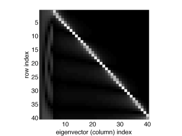
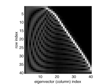
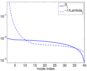
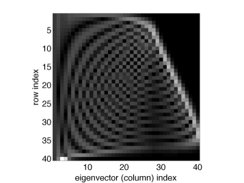
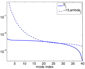
Fig. 2: Waveguide filled with a random medium. Left plots: Absolute values of the entries of the matrix ${\bf U}$ of eigenvectors. Gray scale with lighter color indicates larger values and black indicates nearly zero. The column index is in the abscissa and the row index in the ordinate. Right plots: The scattering mean free path of the modes (full line) and the scales $-1/\Lambda_{j}$, for $j=2,\ldots N$ (dotted line). In the top row $\ell=\lambda_{o}$, in the middle row $\ell=3\lambda_{o}$ and in the last row $\ell=5\lambda_{o}$. These scales should be multiplied by $\varepsilon^{-2}$ e.g., in media with $1\%$ fluctuations, the ordinate is in units of $\times 10^{4}$m.

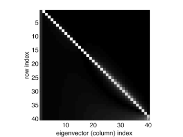
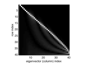
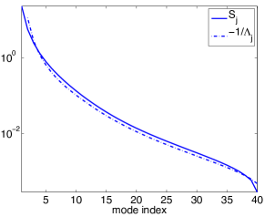
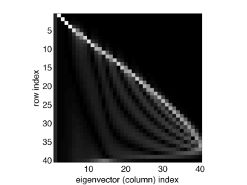
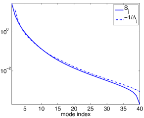
Fig. 3: Waveguide with top random boundary. Left plots: Absolute values of the entries of the matrix ${\bf U}$ of eigenvectors. Gray scale with lighter color indicates larger values and black indicates nearly zero. The column index is in the abscissa and the row index in the ordinate. Right plots: The scattering mean free path of the modes (full line) and the scales $-1/\Lambda_{j}$, for $j=2,\ldots N$ (dotted line). In the top row $\ell=\lambda_{o}$, in the middle row $\ell=3\lambda_{o}$ and in the last row $\ell=5\lambda_{o}$. These scales should be multiplied by $\varepsilon^{-2}$.

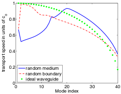
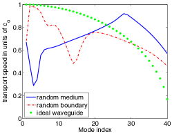
Fig. 4: Transport speeds in waveguide filled with a random medium (solid blue), and with random boundary (dotted red). The speed in ideal waveguides (dotted green). From left to right: $\ell=\lambda_{0}$, $\ell=3\lambda_{o}$ and $\ell=5\lambda_{o}$. The abscissa is mode index and the ordinate is the speed scaled by $c_{o}$.

We display in the left plots of Figures 2 and 3 the absolute values of the entries in the matrix ${\bf U}$ of the eigenvectors, and in the right plots the scattering mean free paths of the modes and the range scales $1/|\Lambda_{j}|$, for $j=2,\ldots,N$. We note that the matrix of eigenvectors has a nearly vanishing block in the upper right corner. Explicitly, there is an index $j_{\star}$ such that the first entries of the eigenvectors ${\bf u}_{j}$ are negligible for $j>j_{\star}$. In the first simulation in Figure 2 $j_{\star}\approx 5$, in the second $j_{\star}\approx 15$ and in the last $j_{\star}\approx 25$. The effect is more pronounced in the case of random boundaries where $j^{\star}\approx 1$ for all three simulations.

The transport speeds are displayed in Figure 4. They are close to the deterministic ones for most of the modes in the case $\ell=\lambda_{o}$, but they are very different when $\ell=5\lambda_{o}$. Thus, it is important to use the transport equations in the range estimation, because the anomalous dispersion induced by scattering may be significant.

In Figure 5 we present inversion results for $\xi(x)=\mathcal{N}(X/4,X/30)$ (left plots) and $\xi(x)=\mathcal{N}(X/4,X/15)$ (right plots). The plots on the top line show the source cross-range profile and the autocorrelation $\mathcal{R}_{\xi}(x)$. The plots in the middle line show the exact values $|\widehat{\xi}_{j}|^{2}$ and the estimated ones for cut-off at $J=30$ and $J=7$, respectively. The estimates are calculated using (72) with regularization (74). In the waveguide filled with a random medium for the cut-off at $J=30$ the array is at $Z_{\mathcal{A}}=\mathcal{L}_{eq}/40$, and for $J=7$ we have $Z_{\mathcal{A}}=\mathcal{L}_{eq}/10.$ The regularization is chosen so that the exponentials in (74) are bounded by $e^{|\Lambda_{j}|Z_{\mathcal{A}}}\lesssim 10,$ for $j=1,\ldots,J.$ The bottom plots show the estimated autocorrelation calculated using equation (76), with the series truncated at $j=J$ and $|\widehat{\xi}_{j}|^{2}$ replaced by the estimates. The results show that the regularization with $J=30$ gives a good approximation of the (first) largest Fourier coefficients and therefore of the autocorrelation. However, the estimates for $J=7$ are poor and give no information about the location of the source (the minimum of the autocorrelation is not evident in the estimates). The standard deviation of the Gaussian centered at zero (the peak of the autocorrelation), which determines the width of the support of the source, is related to the rate of decay of the Fourier coefficients. Thus, we can estimate it even for $J=7$ in the case of the broader source (bottom right plot) but not for the narrower source (bottom left plot).

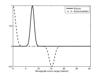
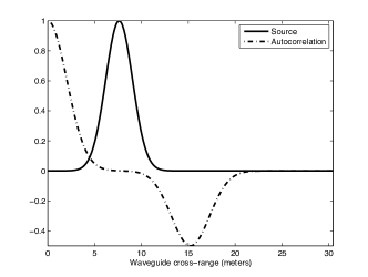
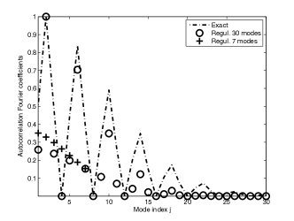
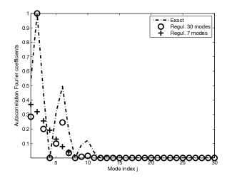
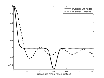
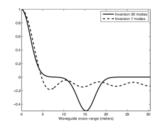
Fig. 5: Left $\xi(x)=\mathcal{N}(x_{o}=X/4,\sigma=X/30)$. Right $\xi(x)=\mathcal{N}(x_{o}=X/4,\sigma=X/15)$. Top line the source cross-range profile $\xi(x)$ (full line) and the autocorrelation $\mathcal{R}_{\xi}(x)$ (dotted line). Middle plots show the exact $|\xi_{j}|^{2}$ and the recovered one for cut-off at $J=30$ (circle) and $J=7$ (cross). Bottom plots show the recovered $\mathcal{R}_{\xi}$ for cut-off at $J=30$ (full line) and $J=7$ (dotted line).

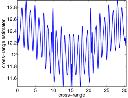
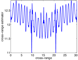
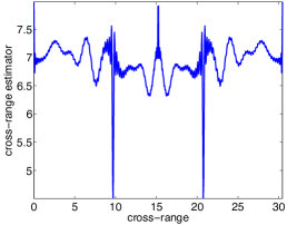
Fig. 6: Estimation of the cross-range location of a point-like source at $X/\pi\approx 9.697\lambda_{o}$ using wideband measurements of the waves in the equipartition regime. Left $\omega\in(\omega_{o},2\omega_{o})$, middle $\omega\in(\omega_{o},3\omega_{o})$ and right $\omega\in(0.5\omega_{o},3\omega_{o})$. Abscissa is cross-range in $\lambda_{o}$ and ordinate is the objective function (87). The minima indicate the location of the source and its mirror image with respect to the center of the waveguide.

The last numerical illustration in Figure 6 demonstrates the benefit of a large bandwidth in the estimation of the cross-range profile of the source at very long ranges, where the measured waves are in the equipartition regime, as discussed in section 5.4. We use the prior knowledge that $\xi(x)\approx\delta(x-x_{o})$, and calculate the objective function

$$\mbox{Obj}(x)=\left\{\sum_{j=1}^{N_{{}_{M}}}\left[\left|\sin\left(\frac{\pi jx}{X}\right)\right|^{2}-{\boldsymbol{\gamma}}\right]^{2}\right\}^{1/2},$$ (87)

where ${\boldsymbol{\gamma}}$ is the solution of the least squares problem

$$\mbox{arg min}\|\mathbb{B}{\boldsymbol{\gamma}}-\left(N_{1}\theta_{1},\ldots N_{{}_{M}}\theta_{{}_{M}})^{T}\right\|^{2}\quad\mbox{such that}~{}{\boldsymbol{\gamma}}\geq{\bf 0},$$ (88)

where the inequality is understood component-wise. We solve (88) with the MATLAB function lsqnonneg. As indicated in the caption of Figure 6 we consider three frequency bands, sampled in steps of $0.02\omega_{o}$. In the first case $\omega\in(\omega_{o},2\omega_{o})$, so $\mathbb{B}\in\mathbb{R}^{50\times 81}$, with rank $50$, and the number of modes ranges from $N_{1}=40$ to $N_{50}=81$. In the second case $\omega\in(\omega_{o},3\omega_{o})$, so $\mathbb{B}\in\mathbb{R}^{100\times 121}$, with rank $92$, and the number of modes ranges from $N_{1}=40$ to $N_{100}=121$. In the last case $\omega\in(0.5\omega_{o},3\omega_{o})$, so $\mathbb{B}\in\mathbb{R}^{125\times 121}$, with rank $110$, and the number of modes ranges from $N_{1}=20$ to $N_{125}=121$. Note how in the last two simulations the minima of the objective function indicate the cross-range location $x_{o}=X/\pi$ of the source and its mirror image with respect to the axis of the waveguide. In the first simulation the bandwidth is not wide enough and the estimation is ambiguous.

5.6 Analysis of the structure of the matrix of eigenvectors

Here we use a simplified model $\Upsilon$ of $\Gamma$ to show with analysis that ${\bf U}$ has a nearly vanishing block in the upper right corner. The model neglects the energy transfer between modes that are not immediate neighbors, meaning that $\Upsilon$ is tridiagonal. It applies to a different regime than that considered in the numerical simulations, so the results complement the previous ones. The regime is for large correlation lengths satisfying

$$k_{o}\ell=O(N),\qquad N\gg 1,$$

so that $\Upsilon$ is a good approximation (up to a multiplicative factor) of $\Gamma$.

The definition of $\Upsilon$ is

$$k_{o}\Upsilon_{jq}=\left\{\begin{array}[]{ll}\Gamma_{jq},&|j-q|=1,\\ 0,&|j-q|>1,\end{array}\right.$$ (89)

for $j\neq q$, and

$$k_{o}\Upsilon_{jj}=\left\{\begin{array}[]{ll}-\Gamma_{jj-1}-\Gamma_{jj+1},&2\leq j\leq N-1,\\ -\Gamma_{12},&j=1,\\ -\Gamma_{N-1N},&j=N.\end{array}\right.$$ (90)

We factor out $k_{o}$ for convenience of the calculations, and use the expression (30) of $\Gamma$ with the assumption that the fluctuations in the medium play the dominant role. Then, the diagonal of $\Upsilon$ scales as

$$\Upsilon_{jj}\sim\frac{N^{2}}{N-j+1},\qquad j=1,\ldots,N.$$ (91)

We summarize the properties of the spectrum of $\Upsilon$ in the next proposition proved in appendix C. We denote its eigenvectors and eigenvalues with the same symbols ${\bf u}_{j}$ and $\Lambda_{j}$. This is an abuse of notation, but the spectrum of $\Gamma$ can be related to that of $\Upsilon$ using known perturbation theory [23].

Proposition 1.

The tridiagonal matrix $\Upsilon$ has the following properties:

1. The eigenvectors form an orthonormal basis of $\mathbb{R}^{N}$ and $\Lambda_{j}\leq 0.$

2. The null space is one dimensional.

3. The norm is $\|\Upsilon\|=O(N^{2}).$

4. $|\Lambda_{j}|=O(N^{2})$ for indices $j$ satisfying $N-j=O(1)$.

5. If $\Lambda_{j}$ is a “large eigenvalue”, meaning that $\delta=N/|\Lambda_{j}|\ll 1$, and $J$ is a spectral cut-off satisfying $J\leq N/2$, we have $\displaystyle\sum_{q=1}^{J}u_{qj}^{2}\leq O(\delta^{2}).$

The first two properties are the same as those stated earlier for $\Gamma$, under the assumption that its off-diagonal entries are strictly positive. The last property confirms our expectation that the matrix ${\bf U}$ has a nearly vanishing upper right corner.

6 Summary

We presented an analysis of the inverse source problem in perturbed two dimensional acoustic waveguides, with data given by time resolved measurements of the pressure field $p(t,\vec{{\bf x}})$ at a remote array of sensors. The waves are trapped by pressure release boundaries and are guided along the the range direction, the axis of the waveguide. The perturbations consist of small scale fluctuations of the boundaries and the sound speed in the medium that fills the waveguide. Such fluctuations cannot be known in detail in practice and are thus modeled with random processes. This places the problem in a stochastic framework. The inversion is carried in a single waveguide, one realization of the random model, and the goal is to obtain robust estimates of the source density $\rho(\vec{{\bf x}})$. Robust means insensitive (statistically stable) with respect to the particular realization of the random perturbations of the waveguide.

Typical imaging methods are based on the assumption that the field $p(t,\vec{{\bf x}})$ is coherent, equal to its statistical expectation plus some small additive noise. This holds approximately in weak scattering regimes i.e., when the array is not too far from the source. We consider strong scattering regimes where $p(t,\vec{{\bf x}})$ is incoherent, it is essentially a random, mean zero field.

Our inversion methodology is based on the theory of wave propagation in random waveguides [20, 10, 13, 14, 4]. This theory decomposes the wave field in a countable set of modes, which are time harmonic propagating and evanescent waves. It models the cumulative wave scattering effects of the perturbations in the waveguide by the mode amplitudes, which are complex valued random fields. We use their statistical description to obtain the following results: (1) We show how to get high fidelity estimates of the energy carried by the modes to the array from cross-correlations of the incoherent data. We explain which cross-correlations are useful and how to calculate them. (2) As the waves propagate and scatter in the random waveguide, they interchange energy. This is described by a system of transport equations with initial condition that depends on the unknown source density $\rho$. We analyze the invertibility of this system. (3) We quantify what can be recovered about the source in terms of the range to the array. The cumulative scattering effects impede the inversion process, and the longer the range, the more pronounced the impediment.

The energies of the propagating modes encode the source information in terms of a matrix of absolute values of Fourier coefficients of $\rho$. It is impossible to determine this matrix uniquely from the estimated energies (the problem is under-determined), unless there is additional information about $\rho$. We assume that it is a separable function $\rho(\vec{{\bf x}})=\xi(x)\zeta(z)$, where $x$ is the cross-range component of $\vec{{\bf x}}$ and $z$ is the range, along the axis of the waveguide. We study in detail two cases: (1) The estimation of the range profile $\zeta(z)$ when the cross-range $\xi(x)$ is known, and (2) The estimation of the cross-range profile $\xi(x)$ when the source has point-like support in range $\zeta(z)=\delta(z)$. Other known range profiles $\zeta(z)$ may be considered as well, but they do not bring new insight to the inversion process. In both cases there is ambiguity about the source, because only the absolute value of the Fourier coefficients of $\zeta(z)$ or $\xi(x)$ can be determined. We can expect only limited information about $\rho(\vec{{\bf x}})$, such as the size of its support in range or cross-range. This can be estimated from the autocorrelation functions of $\zeta(z)$ or $\xi(x)$, which can be approximated using the absolute values of their Fourier coefficients.

The range profile estimation turns out to be the easier of the two cases. We can determine the vector $(|\widehat{\zeta}(\beta_{j})|)_{1\leq j\leq N}$ of absolute values of the Fourier transform of $\zeta(z)$ evaluated at the wavenumbers $\beta_{j}$ of the $N$ propagating modes, and the calculation is well posed no matter how far the array is from the source. The wavenumbers $\beta_{j}$ sample the interval $(0,\omega_{o}/c_{o})$, in steps that decrease monotonically with $N$. Here $\omega_{o}$ is the central frequency of the signal emitted by the source and $c_{o}$ is the reference wave speed in the medium that fills the waveguide. Thus, we can obtain good approximations of the autocorrelation of the range profile $\zeta(z)$, specially in high frequency regimes.

The cross-range estimation entails the calculation of the vector $(|\widehat{\xi}_{j}|)_{1\leq j\leq N}$ of Fourier coefficients of $\xi(x)$. The Fourier basis is defined by the eigenfunctions of the second derivative operator in $x$, which are sin functions in our case. Although the mode energies define uniquely the vector $(|\widehat{\xi}_{j}|)_{1\leq j\leq N}$, the calculation is ill posed and the problem becomes worse as the range separation between the source and the array increases. Cumulative scattering transfers energy between the modes, and the longer the waves travel, the harder it is to determine the initial energy distribution, which is defined by $(|\widehat{\xi}_{j}|)_{q\leq j\leq N}$. There is a range scale, called the equipartition distance $\mathcal{L}_{eq}$, beyond which the energy becomes uniformly distributed between the modes, independent of the initial state. The waves lose all information about the cross-range profile at such ranges, and the inversion for $\xi(x)$ becomes impossible. This is for a narrow frequency band. If a wide frequency band is available, then the estimation of the cross-range profile may be improved.

The analysis in this paper is for two dimensional waveguides with reflecting boundaries. It extends to leaky waveguides where energy is lost by radiation through a boundary, such as the ocean floor. The system of transport equations that models the propagation of energy in such waveguides is derived in [20, Equation (4.3)]. It is almost the same as the system analyzed in this paper, expect that there is damping of energy due to the radiation. This damping adds to the ill posedness of the inversion.

Extensions to three dimensional acoustic waveguides with reflecting boundaries are straightforward, and do not introduce anything new if there are no degeneracies (multiplicity) of the eigenvalues of the Laplacian in the cross-range. It is difficult to quantify such degeneracies for arbitrary cross-sections of the waveguide. But in certain cases like rectangular cross-sections with sides $L_{1}$ and $L_{2}$, degeneracies occur if and only if $L_{1}/L_{2}$ is a rational number. In vectorial problems, such as electromagnetic waveguides, degeneracies are unavoidable for any cross-range profile, because of different states of polarization of the waves [3, 22]. Degeneracies are interesting because they introduce statistical correlations between the amplitudes of the modes that correspond to degenerate eigenvalues. We no longer have scalar valued energies carried by each mode, but Hermitian matrices that describe the propagation of energy by the set of degenerate modes [3]. The transport equations are more complicated [3], but they may lead to extra information about the cross-range profile of the source, not just the absolute value of its Fourier coefficients. However, there is no gain in the stability of the inverse problem. The transfer of energy between the modes occurs in any type of random waveguide, and the estimation of the initial energy state, which determines the cross-range of the source, remains exponentially ill-posed for narrow bandwidths.

Appendix A The model of the cross-correlations

We obtain from (43), (44) and definition (20) that relates the mode amplitudes to the propagator that

$$\widehat{\mathcal{C}}_{j}(h)\approx \,\widehat{\psi}\left(\frac{h}{H}\right)\int_{-\infty}^{\infty}\frac{d\omega}{B^{2}}\left|\widehat{f}\left(\frac{\omega-\omega_{o}}{B}\right)\right|^{2}\sum_{q,q^{\prime}=1}^{N}Q_{jq}Q_{jq^{\prime}}\sum_{l,l^{\prime}=1}^{N}\frac{1}{4\beta_{l}(\omega_{o})\beta_{l^{\prime}}(\omega_{o})}\times$$

$$\int_{-\infty}^{\infty}\frac{du}{2\pi}\,\widehat{\chi}(u)e^{iu{\left[\varepsilon^{2}t_{o}-\beta_{q}^{\prime}(\omega_{o})Z_{{}_{\mathcal{A}}}\right]}/{T}}\int_{-\infty}^{\infty}\frac{du^{\prime}}{2\pi}\,\overline{\widehat{\chi}(u^{\prime})}e^{-iu^{\prime}\left[\varepsilon^{2}t_{o}-\beta_{q^{\prime}}^{\prime}(\omega_{o})Z_{{}_{\mathcal{A}}}\right]/{T}}\times$$

$$\qquad e^{i\frac{Z_{{}_{\mathcal{A}}}}{\varepsilon^{2}}\left\{\beta_{q}(\omega_{o})-\beta_{q^{\prime}}(\omega_{o})+(\omega-\omega_{o})[\beta_{q}^{\prime}(\omega_{o})-\beta^{\prime}_{q^{\prime}}(\omega_{o})]\right\}+ih\beta_{q^{\prime}}^{\prime}(\omega_{o})Z_{{}_{\mathcal{A}}}}\times$$

$$\int_{0}^{X}dx\int_{-\infty}^{\infty}dz\,\rho(x,z)\phi_{l}(x)e^{-i\beta_{q}(\omega)z}\int_{0}^{X}dx^{\prime}\int_{-\infty}^{\infty}dz^{\prime}\,\overline{\rho(x^{\prime},z^{\prime})}\phi_{l^{\prime}}(x^{\prime})e^{i\beta_{q^{\prime}}(\omega)z^{\prime}}\times$$

$$\qquad\mathbb{P}_{ql}^{\varepsilon}\left(\omega-\frac{\varepsilon^{2}u}{T},Z_{{}_{\mathcal{A}}},z^{\prime}\right)\overline{\mathbb{P}_{q^{\prime}l^{\prime}}^{\varepsilon}\left(\omega-\varepsilon^{2}h-\frac{\varepsilon^{2}u^{\prime}}{T},Z_{{}_{\mathcal{A}}},z^{\prime}\right)}.$$ (92)

When we calculate the expectation of (92) using the moment formula (34), we see that only the terms with $q=q^{\prime}$ and $l=l^{\prime}$ survive in the sum. The coherent terms for $q=l$, $q^{\prime}=l^{\prime}$ and $q\neq q^{\prime}$ in the second moment (34) do not appear at full aperture, where $Q_{jq}=\delta_{jq}$. It the array has partial aperture but $\mathcal{A}$ is large enough to have a diagonally dominant matrix $Q$, the coherent terms are small because of the small weights $Q_{jq}$ for $q\neq j$, and specially because of the assumption that $Z_{{}_{\mathcal{A}}}>\mathcal{S}_{1}$. The result is

$${\mathbb{E}}\left[\widehat{\mathcal{C}}_{j}(h)\right]\approx\,\widehat{\psi}\left(\frac{h}{H}\right)\int_{-\infty}^{\infty}\frac{d\omega}{B^{2}}\left|\widehat{f}\left(\frac{\omega-\omega_{o}}{B}\right)\right|^{2}\sum_{q=1}^{N}Q^{2}_{jq}\sum_{l=1}^{N}\frac{\left|\widehat{\rho}_{l}\left[\beta_{q}(\omega)\right]\right|^{2}}{4\beta_{l}(\omega_{o})\beta_{q}(\omega_{o})}\times$$

$$~{}\int_{-\infty}^{\infty}\frac{du}{2\pi}\,\widehat{\chi}(u)\int_{-\infty}^{\infty}\frac{du^{\prime}}{2\pi}\,\overline{\widehat{\chi}(u^{\prime})}e^{i(u-u^{\prime})\varepsilon^{2}t_{o}/T}\widehat{\mathcal{W}}_{q}^{(l)}\left(\omega,h+\frac{u^{\prime}-u}{T},Z_{{}_{\mathcal{A}}}\right),$$ (93)

where $\widehat{\rho}_{k}(\beta)$ are the Fourier coefficients of the source density defined by (48). Taking the inverse Fourier transform of (93) and changing variables $h^{\prime}=h+{(u^{\prime}-u)}/{T}$

$${\mathbb{E}}\left[\mathcal{C}_{j}(\tau)\right]\approx \,\left|\widehat{\chi}\left(\frac{\tau-\varepsilon^{2}t_{o}}{T}\right)\right|^{2}\int_{-\infty}^{\infty}\frac{d\omega}{B^{2}}\left|\widehat{f}\left(\frac{\omega-\omega_{o}}{B}\right)\right|^{2}\sum_{q=1}^{N}Q^{2}_{jq}\times$$

$$\sum_{l=1}^{N}\frac{\left|\widehat{\rho}_{l}\left[\beta_{q}(\omega)\right]\right|^{2}}{4\beta_{l}(\omega_{o})\beta_{q}(\omega_{o})}\int_{-\infty}^{\infty}\frac{dh^{\prime}}{2\pi}\widehat{\mathcal{W}}_{q}^{(l)}\left(\omega,h^{\prime},Z_{{}_{\mathcal{A}}}\right)\widehat{\psi}\left(\frac{h^{\prime}}{H}\right)e^{-ih^{\prime}\tau}.$$ (94)

Here we used that $\psi$ is smooth and $HT\gg 1$, to approximate

$$\widehat{\psi}\left(\frac{h^{\prime}}{H}-\frac{u^{\prime}-u}{TH}\right)\approx\widehat{\psi}\left(\frac{h^{\prime}}{H}\right).$$

Equation (47) follows from (94) and definition (37) of the Wigner transform. We also use that the bandwidth is small and that the Fourier transform $\widehat{f}$ of the pulse and $\widehat{\rho}_{l}(\beta)$ are smooth in $\omega$. In fact the latter is analytic because $\rho$ has compact support.

To assess the statistical stability of $\mathcal{C}_{j}(\tau)$ we need the fourth order moments of the propagator. These are given in [8, Appendix D], and the variance of $\mathcal{C}_{j}(\tau)$ follows after a long calculation which we explain briefly. Since it is defined by

$${\rm var}\left[\mathcal{C}_{j}(\tau)\right]={\mathbb{E}}\left[\left|\mathcal{C}_{j}(\tau)\right|^{2}\right]-\left|{\mathbb{E}}\left[\mathcal{C}_{j}(\tau)\right]\right|^{2},$$

we need fourth order moments like

$${\mathbb{E}}\left[\mathbb{P}_{q_{1}l_{1}}^{\varepsilon}\left(\omega,Z_{{}_{\mathcal{A}}},z_{1}\right)\overline{\mathbb{P}_{q_{2}l_{2}}^{\varepsilon}\left(\omega,Z_{{}_{\mathcal{A}}},z_{2}\right)}\mathbb{P}_{q^{\prime}_{1}l^{\prime}_{1}}^{\varepsilon}\left(\omega^{\prime},Z_{{}_{\mathcal{A}}},z^{\prime}_{1}\right)\overline{\mathbb{P}_{q^{\prime}_{2}l^{\prime}_{2}}^{\varepsilon}\left(\omega^{\prime},Z_{{}_{\mathcal{A}}},z^{\prime}_{2}\right)}\right]$$

where we neglect the order $\varepsilon^{2}$ offsets in the arguments, because they do not play any role. These moments factorize in the product of two second moments at frequencies $\omega$ and $\omega^{\prime}$ when $|\omega^{\prime}-\omega|\gg\varepsilon^{2}\omega_{o}$, so in the calculation of the variance we are left with the integration over the small strip $\{\omega,\omega^{\prime}:~{}~{}|\omega-\omega^{\prime}|\ll\varepsilon^{2}\omega_{o}\}$. This makes the variance smaller than the square of the mean (47), by a factor of $\varepsilon^{2}\omega_{o}/B=\varepsilon^{2-\alpha}\ll 1$, as long as the mean is large. This happens for example when the matrix $Q$ is diagonally dominant and we evaluate the cross-correlation at a time $\tau$ for which $\mathcal{W}_{j}^{(l)}$ is large.

Appendix B Justification of the perturbative analysis of arrival times

To show that $ih\mathfrak{B}^{\prime}+\Gamma$ is a perturbation of $\Gamma$ for $|h|\leq H$, let us calculate the ratio $|\Gamma_{jj}|/(H\beta^{\prime}_{j})$ for $j=1,\ldots,N$.

Using (30) and the definition of $\beta_{j}$ we have

$$\frac{|\Gamma_{jj}|}{H\beta^{\prime}_{j}}=\frac{\omega_{o}}{H}\frac{\pi^{4}\ell j^{2}}{k_{o}^{2}X^{4}}\sum_{q\neq j}\frac{q^{2}}{\beta_{q}}\left\{\widehat{\mathcal{R}}_{{}_{B}}\left[\ell(\beta_{j}-\beta_{q})\right]+\widehat{\mathcal{R}}_{{}_{T}}\left[\ell(\beta_{j}-\beta_{q})\right]\right\}+$$

$$\frac{\omega_{o}}{H}\frac{k_{o}^{2}\ell}{4}\sum_{q\neq j}\frac{1}{\beta_{q}}\widehat{\mathcal{R}}_{\nu_{jq}}\left[\ell(\beta_{j}-\beta_{q})\right],$$ (95)

and we estimate next each term. For the first term

$$T_{1}=\frac{\omega_{o}}{H}\frac{\pi^{4}\ell j^{2}}{k_{o}^{2}X^{4}}\sum_{q\neq j}\frac{q^{2}}{\beta_{q}}\widehat{\mathcal{R}}_{{}_{B}}\left[\ell(\beta_{j}-\beta_{q})\right]$$ (96)

we use that $\pi/X\approx k/N$ and $\beta_{q}\approx k\sqrt{1-(q/N)^{2}},$ to write

$$T_{1} \approx\frac{\omega_{o}}{H}\frac{k_{o}\ell j^{2}}{N}\frac{1}{N}\sum_{q\neq j}\frac{(q/N)^{2}}{\sqrt{1-(q/N)^{2}}}\widehat{\mathcal{R}}_{{}_{B}}\left[k_{o}\ell(\sqrt{1-(j/N)^{2}}-\sqrt{1-(q/l)^{2}})\right]$$

$$\approx\frac{\omega_{o}}{H}\frac{k_{o}\ell j^{2}}{N}\int_{0}^{1}du\,\frac{u^{2}}{\sqrt{1-u^{2}}}\widehat{\mathcal{R}}_{{}_{B}}\left[k_{o}\ell(\sqrt{1-(j/N)^{2}}-\sqrt{1-u^{2}})\right].$$

Moreover, changing variables $s=\sqrt{1-(j/N)^{2}}-\sqrt{1-u^{2}},$ we obtain

$$T_{1}\approx\frac{\omega_{o}}{H}\frac{k_{o}\ell j^{2}}{N}\int ds\left[1-(s-\sqrt{1-(j/N)^{2}})^{2}\right]^{1/2}\widehat{\mathcal{R}}_{{}_{B}}(k_{o}\ell s)=O\left(\frac{\omega_{o}}{H}\frac{j^{3}}{N^{2}}\right).$$ (97)

The second term in (95) is similar to $T_{1}$ and to estimate the third term we need

$$\widehat{\mathcal{R}}_{\nu_{jq}}\left[\ell(\beta_{j}-\beta_{l})\right]=\frac{4}{X^{4}}\int d\eta\,e^{i\ell(\beta_{j}-\beta_{q})\eta}\int_{0}^{X}dx_{1}\int_{0}^{X}dx_{2}\,\sin\left(\frac{\pi jx_{1}}{X}\right)\times$$

$$\sin\left(\frac{\pi jx_{2}}{X}\right)\sin\left(\frac{\pi qx_{1}}{X}\right)\sin\left(\frac{\pi qx_{2}}{X}\right)\mathcal{R}_{\nu}\left(\frac{x_{2}-x_{1}}{\ell},\eta\right),$$

where we assume that the fluctuations $\nu$ are stationary in both range and cross-range. Changing variables to $\bar{x}=(x_{1}+x_{2})/2$ and $\tilde{x}=x_{2}-x_{1},$ we have using basic trigonometry

$$\widehat{\mathcal{R}}_{\nu_{jq}}\left[\ell(\beta_{j}-\beta_{l})\right]\approx\frac{\ell}{X}\int d\eta\,e^{i\ell(\beta_{j}-\beta_{q})\eta}\int_{-X/\ell}^{X/\ell}\frac{d\tilde{x}}{\ell}\cos\left(\frac{\pi j\tilde{x}}{X}\right)\cos\left(\frac{\pi q\tilde{x}}{X}\right)\mathcal{R}_{\nu}\left(\frac{\tilde{x}}{\ell},\eta\right).$$

Moreover, assuming that $X\gg\ell$ we can approximate the last integral by the Fourier transform of $\mathcal{R}_{\nu}$ in the first argument, denoted by $\breve{\mathcal{R}}_{\nu}$, and get

$$\widehat{\mathcal{R}}_{\nu_{jq}}\left[\ell(\beta_{j}-\beta_{l})\right] \approx\frac{\ell}{2X}\int d\eta\,e^{i\ell(\beta_{j}-\beta_{q})\eta}\left[\breve{\mathcal{R}}_{\nu}\left(\frac{k\ell(j-q)}{N},\eta\right)+\breve{\mathcal{R}}_{\nu}\left(\frac{k\ell(j-q)}{N},\eta\right)\right]$$

$$=\frac{\ell}{2X}\left[\widehat{\mathcal{R}}_{\nu}\left(\frac{k\ell(j-q)}{N},\ell(\beta_{j}-\beta_{q})\right)+\widehat{\mathcal{R}}_{\nu}\left(\frac{k\ell(j-q)}{N},\ell(\beta_{j}-\beta_{q})\right)\right].$$

The third term in (95) becomes

$$T_{3} =\frac{\omega_{o}}{H}\frac{k_{o}^{2}\ell}{4}\sum_{q\neq j}\frac{1}{\beta_{q}}\widehat{\mathcal{R}}_{\nu_{jq}}\left[\ell(\beta_{j}-\beta_{q})\right]$$

$$=\frac{\omega_{o}}{H}\frac{(k_{o}\ell)^{2}}{8\pi}\frac{1}{N}\sum_{q\neq j}\left[\widehat{\mathcal{R}}_{\nu}\left(\frac{k\ell(j-q)}{N},\ell(\beta_{j}-\beta_{q})\right)+\widehat{\mathcal{R}}_{\nu}\left(\frac{k\ell(j-q)}{N},\ell(\beta_{j}-\beta_{q})\right)\right]$$

$$\approx\frac{\omega_{o}}{H}\frac{(k_{o}\ell)^{2}}{8\pi}\int_{0}^{1}\frac{du}{\sqrt{1-u^{2}}}\widehat{\mathcal{R}}_{\nu}\left(k\ell(j/N-u),k_{o}\ell(\sqrt{1-(j/N)^{2}}-\sqrt{1-u^{2}})\right)$$

$$=O\left(\frac{\omega_{o}}{H}k_{o}\ell\right),$$ (98)

where we used that $k_{o}\ell\gg 1$ in forward scattering approximation regimes. Indeed, the forward scattering approximation requires that [20, 13, 4]

$$\widehat{\mathcal{R}}_{\nu_{j}q}[\ell(\beta_{j}+\beta_{q})]\ll 1,\qquad\forall~{}j,q=1,\ldots,N,$$

which implies $k_{o}\ell\gg 1$.

Gathering the results (95)-(98) we see that

$$\frac{|\Gamma_{jj}|}{H\beta^{\prime}_{j}}=\frac{\omega_{o}}{H}\left[O\left(\frac{j^{3}}{N^{2}}\right)+O(k_{o}\ell)\right].$$ (99)

The second term is due to the the fluctuations in the medium and is large when $H\sim\omega_{o}$ because $k_{o}\ell\gg 1$. The first term is due to the fluctuations of the boundary and is large for $j\gg N^{2/3}$. In either case, the Frobenius norm of $\Gamma$ is much larger than that of $H\mathfrak{B}^{\prime}$, so we have a matrix perturbation problem. To illustrate the accuracy of the perturbation analysis, we display in Figure 7 the relative error of the approximation of the eigenvalues for the simulations in section 5.5.

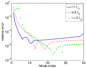
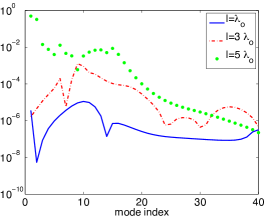
Fig. 7: Relative error of the predicted eigenvalues by the regular perturbation theory equation (51). Waveguide filled with a random medium (left plot) and with a random top boundary (right plot). The abscissa is mode index.

Appendix C Proof of Proposition 1

That the eigenvectors form an orthonormal basis follows from the symmetry of $\Upsilon$. We also obtain from (89)-(90) that the quadratic forms of $\Upsilon$ are

$${\bf v}^{T}\Upsilon{\bf v}=-\sum_{j=2}^{N}\Upsilon_{jj-1}\left(v_{j}-v_{j-1}\right)^{2}\leq 0,\qquad\forall~{}{\bf v}=(v_{1},\ldots,v_{N})^{T}\in\mathbb{R}^{N},$$

so the eigenvalues must satisfy $\Lambda_{j}\leq 0.$ We order them as $0=\Lambda_{1}\geq\Lambda_{2}\geq\ldots\Lambda_{N}$.

We have $(1,1,\ldots,1)^{T}\in{\rm Null}(\Upsilon)$ by construction. To prove property 2, we take a large enough $\gamma$ so that all the entries in the matrix $\Upsilon_{{}_{\gamma}}=\Upsilon+\gamma I$ are positive. This matrix is of Perron-Frobenius type, and its eigenvalues are equal to $\Lambda_{j}+\gamma$. The largest eigenvalue $\Lambda_{o}+\gamma$ is simple, and therefore the null space of $\Upsilon$ is one dimensional.

The variational definition of $|\Lambda_{N}|$ as the maximum of the Rayleigh quotient of $-\Upsilon$ gives that $|\Lambda_{N}|$ is larger than $|\Upsilon_{jj}|$, for any $j=1,\ldots,N$. But $\Upsilon_{NN}=O(N^{2})$ by (91), and property 3 follows from $\|\Upsilon\|=|\Lambda_{N}|.$

Consider square blocks $\Upsilon_{m}$ of $\Upsilon$, containing the last $m=O(1)$ elements on its diagonal. By (91) they scale like $\Upsilon_{m}=N^{2}\widetilde{\Upsilon}_{m},$ where $\widetilde{\Upsilon}_{m}$ have entries of order one. Cauchy’s interlacing theorem gives that $|\Lambda_{N-m+j}|\geq N^{2}|\widetilde{\lambda}_{j}|$, for $j=1,\ldots,m,$ where $\widetilde{\lambda}_{j}\leq 0$ are the eigenvalues of $\widetilde{\Upsilon}_{m}$ in decreasing order. To prove Property 4 it remains to show that these are all $O(1)$. First, let us see that $\widetilde{\Upsilon}_{m}$ has a trivial null space. Indeed, suppose that ${\bf v}\in{\rm Null}(\widetilde{\Upsilon}_{m})$ and write equation $\widetilde{\Upsilon}_{m}{\bf v}={\bf 0}$ row by row. Starting from the last row to the second, and using definitions (89)-(90), we obtain that all entries in ${\bf v}$ must be equal to say $v$. However, the first equation gives that $v=0$, because the elements in the first row of $\widetilde{\Upsilon}_{m}$ do not add to zero. Thus, the null space is trivial. The smallest in magnitude eigenvalue equals the minimum of the Rayleigh quotient

$$\frac{{\bf v}^{T}(-\widetilde{\Upsilon}_{m}){\bf v}}{{\bf v}^{T}{\bf v}}=\left[\widetilde{\beta}_{N-m}v_{1}^{2}+\displaystyle\sum_{j=1}^{m-1}\widetilde{\beta}_{N-m+j}(v_{j+1}-v_{j})^{2}\right]/{\displaystyle\sum_{j=1}^{N}v_{j}^{2}},$$

where $\widetilde{\beta}_{j}=\beta_{j}/N^{2}=O(1)$ and the right hand side is obtained by direct calculation. All the terms in this expression are non-negative and at least one of them must be $O(1)$. Thus, we see that $|\widetilde{\lambda}_{j}|\geq O(1)$ and property 4 follows.

To prove the last property, let $\Lambda$ be a large eigenvalue of $\Upsilon$ and ${\bf u}$ its associated eigenvector. We see from definition (89)-(90) that $|\Upsilon_{jj}|\geq\Upsilon_{jj\pm 1}$, and using that

$$|\Lambda|u_{j}=-\Upsilon_{jj-1}u_{j-1}+|\Upsilon_{jj}|u_{j}-\Upsilon_{jj+1}u_{j+1},$$

we obtain the bound

$$|\Upsilon_{jj}|\left(|u_{j-1}|+|u_{j}|+|u_{j+1}|\right)\geq|\Lambda||u_{j}|.$$

Moreover, multiplying by $|u_{j}|$ and summing over $j=2,\ldots,J$ we get the estimate

$$\sum_{j=2}^{J}u_{j}^{2} \leq|\Lambda|^{-1}\sum_{j=2}^{J}|\Upsilon_{jj}|\left(|u_{j-1}u_{j}|+u_{j}^{2}+|u_{j+1}u_{j}|\right)$$

$$\leq\frac{C\delta N}{N+1-J}\sum_{j=2}^{J}\left(|u_{j-1}u_{j}|+u_{j}^{2}+|u_{j+1}u_{j}|\right),$$

with the second inequality implied by (91) and $1/|\Lambda|=\delta/N$. Since $J\leq N/2$, we have $N/(N+1-J)\leq 2$. Now use Young’s inequality

$$|u_{j}u_{j\pm 1}|\leq\frac{\widetilde{\delta}u_{j\pm 1}^{2}}{2}+\frac{u_{j}^{2}}{2\widetilde{\delta}},$$

which holds for any $\widetilde{\delta}>0$. We let $\widetilde{\delta}=C\delta/4$ and obtain that

$$\sum_{j=2}^{J}u_{j}^{2} \leq C\delta\sum_{j=2}^{J}\left[\delta\left(u_{j-1}^{2}+u_{j+1}^{2}\right)+2\left(1+\frac{1}{4C\delta}\right)u_{j}^{2}\right]$$

or, equivalently,

$$\sum_{j=2}^{J}u_{j}^{2} \leq\frac{4C\delta^{2}}{1-4C\delta-4c\delta^{2}}(u_{1}^{2}+u_{J+1}^{2})\leq\frac{4C\delta^{2}}{1-4C\delta-4c\delta^{2}}.$$

The last inequality is because $\|{\bf u}\|=1$. It remains to show that $|u_{1}|\sim\delta$. This follows from $|\Upsilon_{11}|(u_{1}-u_{2})=|\Lambda|u_{1},$ the estimate (91) that gives $|\Upsilon_{11}|=O(N)$, and the assumption $|\Lambda|=\delta/N$.

References

- [1] SH Abadi, D Rouseff, and DR Dowling. Blind deconvolution for robust signal estimation and approximate source localizationa). Journal of the Acoustical Society of America, 131(4):2599–2610, 2012.
- [2] DS Ahluwalia, JB Keller, and BJ Matkowsky. Asymptotic theory of propagation in curved and nonuniform waveguides. Journal of the Acoustical Society of America, 55(1):7–12, 1974.
- [3] R Alonso and L Borcea. Electromagnetic wave propagation in random waveguides. submitted. Preprint arXiv:1310.4890v1 [math-ph].
- [4] R Alonso, L Borcea, and J Garnier. Wave propagation in waveguides with random boundaries. Commun. Math. Sci., 11:233–267, 2012.
- [5] AB Baggeroer, WA Kuperman, and PN Mikhalevsky. An overview of matched field methods in ocean acoustics. Oceanic Engineering, IEEE Journal of, 18(4):401–424, 1993.
- [6] L Borcea and J Garnier. Paraxial coupling of propagating modes in three-dimensional waveguides with random boundaries. SIAM Multiscale Model Simul, 12(2):832–878, 2014.
- [7] L Borcea, J Garnier, and C Tsogka. A quantitative study of source imaging in random waveguides. Commun Math Sci, 2014, in press. Preprint arXiv: 1306.1544v1.
- [8] L Borcea, L Issa, and C Tsogka. Source localization in random acoustic waveguides. SIAM Multiscale Model Simul, 8:1981–2022, 2010.
- [9] L Borcea, H Kang, H Liu, G Uhlmann. H Ammari, and J Garnier ed. Inverse Problems and Imaging, volume 44 of Panoramas & Synthéses. Societé Mathématique de France, 2014.
- [10] LB Dozier and FD Tappert. Statistics of normal mode amplitudes in a random ocean. J Acoust Soc Am, 63:533–547, 1978.
- [11] S Félix and V Pagneux. Multimodal analysis of acoustic propagation in three-dimensional bends. Wave Motion, 36(2):157–168, 2002.
- [12] J-P Fouque, J Garnier, G Papanicolaou, and K Sølna. Wave propagation and time reversal in randomly layered media. Springer, 2007.
- [13] J Garnier and G Papanicolaou. Pulse propagation and time reversal in random waveguides. SIAM J Appl Math, 67(6):1718–1739, 2007.
- [14] J Garnier and K Sølna. Effective transport equations and enhanced backscattering in random waveguides. SIAM Journal on Applied Mathematics, 68(6):1574–1599, 2008.
- [15] GH Golub and CF Van Loan. Matrix computations, volume 3. JHU Press, 2012.
- [16] C Gomes and K Sølna. Wave propagation in random waveguides with long-range correlations. work in progress.
- [17] C Gomez. Wave propagation in underwater acoustic waveguides with rough boundaries. Preprint arXiv: 0911.5646 [math AP].
- [18] C Gomez. Wave propagation in shallow-water acoustic random waveguides. Commun Math Sci, 9:81–125, 2011.
- [19] KD Heaney and WA Kuperman. Very long-range source localization with a small vertical array. Journal of the Acoustical Society of America, 104:2149, 1998.
- [20] J B Keller and J S Papadakis, editors. Wave propagation in a randomly inhomogeneous ocean, volume 70. Springer Verlag, Berlin, 1977.
- [21] JL Krolik. Matched-field minimum variance beamforming in a random ocean channel. Journal of the Acoustical Society of America, 92:1408, 1992.
- [22] D Marcuse. Theory of dielectric optical waveguides. Quantum electronics–principles and applications. Academic Press, 1991.
- [23] BN Parlett. The symmetric eigenvalue problem, volume 7. SIAM, 1980.
- [24] Lu Ting and Michael J Miksis. Wave propagation through a slender curved tube. Journal of the Acoustical Society of America, 74(2):631–639, 1983.
- [25] K Yoo and TC Yang. Broadband source localization in shallow water in the presence of internal waves. Journal of the Acoustical Society of America, 106:3255, 1999.