Critical behavior of a quantum chain with four-spin interactions in the presence of longitudinal and transverse magnetic fields

Abstract

We study the ground-state properties of a spin-1/2 model on a chain containing four-spin Ising-like interactions in the presence of both transverse and longitudinal magnetic fields. We use entanglement entropy and finite-size scaling methods to obtain the phase diagrams of the model. Our numerical calculations reveal a rich variety of phases and the existence of multi-critical points in the system. We identify phases with both ferromagnetic and anti-ferromagnetic orderings. We also find periodically modulated orderings formed by a cluster of like-spins followed by another cluster of opposite like-spins. The quantum phases in the model are found to be separated by either first or second order transition lines.

I Introduction

There has recently been considerable effort to understand magnetic phase transitions in quantum systems described by Hamiltonians with multi-spin interactions. Ultra cold atoms trapped in optical lattices under idealized laboratory conditions in particular are suitable to simulate these systems  Sim11 ; Jac98 ; Kas95 ; Gre02 ; Man03 ; Pac04 ; Pac04b . A variety of spin Hamiltonians have been physically realized on optical lattices, making possible the experimental study of the zero temperature phase diagrams of those systems.

Recently, Simon at al. Sim11 presented a detailed procedure for the experimental realization of Ising anti-ferromagnetic spin chains in the presence of longitudinal and transverse magnetic fields. Their work opened new possibilities for the investigation of quantum magnetism and criticality in these systems.

Besides the usual competition between various magnetic ordered ground-states, such as ferromagnets, antiferromagnets and paramagnets, the advent of optical lattices allow the study of more complex interactions that give rise to novel ground-state properties in magnetic systems Pac04b ; DCr04 . The presence of higher order spin interactions usually induces unusual properties not found in regular spin systems, bringing out a richer criticality.

Theoretical investigations of quantum phase transitions in magnetic spin chains with three- and four-spin exchange interactions have revealed novel phases and ground-states with multiple periodic structures and unique entanglement properties DCr04 ; Pen84 ; Bon06 ; Bon13 . In particular, the influence of magnetic fields on low-dimensional quantum spin systems with complex interactions is a subject of great interest that may lead to the observation of reentrant behaviors and high-field driven transitions McC11 ; Que12 .

The remarkable success of the experimental work in optical lattices simulating these spin systems has contributed significantly to the renewed interest in the theoretical study of these quantum models. To our knowledge, the effects of an additional longitudinal magnetic field on the ground-state properties of the four-spin quantum chain in a transverse magnetic field has never been investigated and is the subject of this paper. Our aim is to obtain the phase diagrams and to understand the nature of the phase transitions and ground-state properties of the model.

II The Model

Consider a spin-1/2 magnetic chain with periodic boundary conditions. The spins are subjected to a magnetic field with components in the longitudinal and transverse directions. The interaction among the spins is dictated by a four-spin Ising-like term. The Hamiltonian of the system may be written as:

$${\cal H}=-J_{4}\sum_{i}\sigma^{z}_{i}\sigma^{z}_{i+1}\sigma^{z}_{i+2}\sigma^{z}_{i+3}-H_{x}\sum_{i}\sigma^{x}_{i}-H_{z}\sum_{i}\sigma^{z}_{i}.$$ (1)

Here, $\sigma^{\alpha}_{i}$ ($\alpha=x,y,z$) are the components of the Pauli operator, located at site $i$. The parameter $J_{4}$ is the Ising-like four-spin interaction strength. The uniform magnetic field has components $H_{\rm x}$ and $H_{\rm z}$ along the transverse and longitudinal directions, respectively.

For $H_{\rm x}=0$ quantum fluctuations are absent, however, depending on the values of fields and couplings,the model may show a variety of phases. For instance, when the four-spin coupling $J_{4}>0.0$, the sign of the longitudinal field $H_{\rm z}$ determines the direction of the magnetization. For $H_{\rm z}>0$, the system shows a classical ferromagnetic phase with all the spins aligned in the $+z$-direction, the F($+z$) phase. On the other hand, if $H_{\rm z}<0$, the ensuing phase has net magnetization along the $-z$-direction, the F($z$) phase.

The case where $J_{4}<0$ shows four phases, namely the ferromagnetic F($\pm z$) and $<$3,1$>$$(\pm)$ phases. The latter are formed by three consecutive up (down) spins followed by one down (up) spin. There is a transition point at $(H_{z},H_{x})=(0.0,0.0)$ between the $<$3,1$>$$(+)$ and $<$3,1$>$$(-)$ phases, as well as at $H_{\rm z},H_{\rm x})=(\pm 4.0,0.0)$, separating the $<$3,1$>$$(+)$ from the F(+$z$) and the $<$3,1$>$$(-)$ from the F($-z$) phases. The particular case of the transverse four-spin Ising model ($H_{\rm x}\neq 0$ and $H_{\rm z}=0$) was shown to be self-dual, with critical points at $J_{4}/H_{\rm x}=\pm 1$ Tur82 ; Pen82 .

In this paper we investigate the ground-state properties of the Hamiltonian model (Eq. 1) by using two numerical methods: entanglement entropy and finite-size scaling. The first method is based on the behavior of von Neumann entanglement entropy, which is mostly used in information theory. That method enables one to calculate the location of the quantum critical points with a relatively high degree of accuracy, as well as it provides a way to identify the nature of the transitions. In addition, the method makes it possible to determine the central charge of the associated conformal field theory with low computational cost, by using small lattice sizes Xav11 ; Nish11 . The second method is based on finite-size scaling arguments, which can be used to determine the transition lines and global properties of the various ground-states Gui02 .

III The Methods

III.1 Entropy entanglement

In this section we describe the entropy entanglement method and show how to use it to locate the boundary between quantum phases, and how to find the central charge of the associated conformal field theory.

Consider a spin chain of length $L$ that can be partitioned into two subsystems $\cal A$ and $\cal B$ of sizes $L_{\cal A}=l$ and $L_{\cal B}=L-l$, respectively. When the entire system is in a pure state $|\psi\rangle$, its entropy is zero. However, the entropy of each subsystem is finite and can be quantified by the von Neumann entropy, defined as:

$${S}(L,l)=-\textrm{Tr}\left(\rho_{\cal A}\ln\rho_{\cal A}\right)=-\textrm{Tr}\left(\rho_{\cal B}\ln\rho_{\cal B}\right),$$ (2)

where $\rho_{\cal A(\cal B)}=\textrm{Tr}_{\cal B(\cal A)}\,\rho$ denotes the reduced density matrix of $\cal A(\cal B)$ and $\rho=|\psi\rangle\langle\psi|$ is the density matrix of the pure state. The von Neumann entropy $S(L,l)$ gives a reliable measure of the entanglement between the subsystem $\cal A$ and the rest of the system $\cal B$.

For finite systems, Calabrese and Cardy Cal04 showed that conformal invariance implies a diverging logarithmic scaling for the entanglement entropy. In particular, for a one dimensional system of size $L$ with imposed periodic boundary conditions, it assumes the form:

$${S}(L,l)=\frac{c}{3}\ln[\frac{L}{\pi}\sin(\frac{\pi l}{L})]+\beta,$$ (3)

where $c$ is the central charge of the underlying conformal field theory and $\beta$ is a non-universal constant which depends on the model being used.

To locate the boundary between possible quantum phases, we first calculate the entanglement entropy difference between two subsystems with sizes $l$ and $l^{\prime}$ Xav11 ; Nish11 :

$$\Delta{S}={S}(L,l)-{S}(L,l^{\prime})$$ (4)

where $L$ is the size of the spin system.

Consider initially a system that undergoes a second-order phase transition when a parameter $\lambda$ of its Hamiltonian reaches a critical value $\lambda_{c}$. If the system is finite, the entanglement entropy difference remains finite for all values of $\lambda$, reaching a maximum at $\lambda_{c}$. As the size of the system $L$ is increased, the peak of $\Delta S$ at $\lambda_{c}$ becomes progressively narrower. Its value at the transition tends to a finite value, whereas its value elsewhere tends to zero.

Next consider the case of a system that undergoes a first-order transition. Although $\Delta S$ still shows a maximum at the transition point, it diminishes everywhere as $L\rightarrow\infty$. Such behavior of the entanglement entropy difference is used as an indicator of the boundary between two phases and to identify the nature of the transition at that point.

In the scaling regime, where Eq. 3 is valid, we have $1<<l,l^{\prime}<<L$. As a practical matter, to fulfill these conditions and minimize finite-size effects, we choose $l=L/2$ and $l^{\prime}=L/4$ in our calculations Xav11 . Using these values for the subsystems sizes and Eqs. 3 and 4, we obtain:

$$c=6\,{\Delta S}/\ln(2)\,.$$ (5)

A systematic increase of the system size $L$ and the subsequent extrapolation to the infinite-size limit will provide an estimation of the value of the central charge.

III.2 Finite-size scaling

The finite-size scaling method is another way to locate the boundaries between different quantum phases. This method requires knowledge of the first two lowest energy states of the Hamiltonian, $E_{0}$ and $E_{1}$.

Consider again a Hamiltonian model that depends on a parameter $\lambda$ that becomes critical at $\lambda_{c}$. It has been pointed out Bar93 that for a system undergoing a second-order phase transition, the energy gap between the two lowest energy states of the system, $G(\lambda)=E_{1}(\lambda)-E_{0}(\lambda)$, vanishes at the infinite-size limit. For a finite system, at criticality it obeys the following power-law dependence with the size $L$ of the system:

$$G(L,\lambda_{c})\equiv[E_{1}(L,\lambda_{c})-E_{0}(L,\lambda_{c})]\propto L^{-z}.$$ (6)

Here $z$ represents the dynamical critical exponent of the system Bar93 which, for one-dimensional systems that are conformal invariant, equals to one. For simplicity, from now on we set $z=1$ in all expressions in which it appears.

The finite-size estimation of the critical parameter $\lambda_{c}(L,L^{\prime})$ is dependent on the choice of the two system sizes $L$ and $L^{\prime}$. The critical point is then found as a solution of the phenomenological renormalization equation:

$$LG(L,\lambda_{c})={L^{\prime}}G(L^{\prime},\lambda_{c}).$$ (7)

The infinite-size value of the critical parameter is calculated by extrapolating the values obtained from Eq. 7 using increasingly larger system sizes $L$ and $L^{\prime}$.

The ground-state and the first excited state energies and their corresponding eigenstates are calculated as a function of $\lambda$ by using a modified Lanczos method Dag85 . To speed up the calculations we use trial initial vectors which are as close as possible to the actual ground state vectors. The eigenvectors and eigenvalues for the ground-states are determined with precision between $10^{-10}$ and $10^{-12}$. The same quantities for the first excited states are obtained with precision between $10^{-5}$ to $10^{-6}$.

To identify the nature of each phase we need to examine the corresponding ground-state eigenvectors. We start by writing the Hamiltonian on a basis that consists of the product of the eigenstates $|s>_{i}$ ($s=0,1$) of the spin operator $S_{i}^{z}$, $i=1,\dots,L$. Here the labels $s=0$ and $s=1$ correspond to the z-component of the spin state at the site $i$, pointing down and up respectively. Now, an arbitrary basis state of the full Hamiltonian can be written as $|n>=\prod_{i}^{L}\,|s>_{i}$, with the basis state labels $n=0,1,...,N-1$, where $N=2^{L}$ determines the dimension of the Hilbert space for a given system size $L$. An arbitrary state of the system can now be written as:

$$|\psi_{\alpha}>=\sum_{n=0}^{N-1}b_{\alpha}(n)|n>,$$ (8)

where $\alpha=0$ labels the ground-state, and $\alpha=1$ the first excited state. The coefficients $b_{\alpha}(n)$ are the amplitudes of each of the basis states $|n$$>$, of the linear combination forming the arbitrary state $|\psi_{\alpha}>$. Those coefficients are all real, since the Hamiltonian matrix is real and symmetric.

Figure 1: Phase diagram in the $(H_{\rm z}$-$H_{\rm x}$)-plane for $J_{4}=1.0$. The triangles separate a field induced ferromagnetic phase with net magnetization in the $x$-direction, F($+x$), from two induced phases with magnetizations along the $\pm z$-directions, F(+$z$) and F($-z$). The crosses separate the ferromagnetic phases along $\pm z$. All the transition lines are of first order. The data shown were obtained with the entanglement entropy method.

The basis state labels $n$, can be written in binary notation with $L$ digits. The $i$-th position and the value of these digits coincide with the eigenstate of ${S_{i}^{z}}$ at that site. By plotting the coefficients $b_{\alpha}(n)$ as a function of the basis label $n$, we obtain a representation of the quantum state on a single graph and a full characterization of the nature of that state Bon06 .

IV Results

We have carried out numerical calculations to investigate the quantum phase transitions of the Hamiltonian, Eq. 1, using the methods of entanglement entropy and finite-size scaling. We considered chains containing up to 24 spins, and used periodic boundary conditions.

First we set $J_{4}=1.0$ and search for phase transitions by varying the magnetic field components $H_{\rm z}$ and $H_{\rm x}$. Our numerical results for the phase diagram in the ($H_{z}$-$H_{x}$)-plane are shown in Fig. 1. The transition lines (with triangles) separate a ferromagnetic phase with net magnetization in the $x$-direction F($+x$) from two ferromagnetic phases F($+z$) and F($-z$) with spins aligned along the $+z$ and $-z$ directions, respectively.

In the absence of the four-spin interaction, the phase transition lines in Fig. 1 would be along the lines $H_{\rm x}=\pm H_{\rm z}$. Under the present conditions however, the field $H_{z}$ reinforces the ferromagnetic order caused by the four-spin interaction. Therefore, it takes a larger transverse field $H_{x}$ to change the direction of the net magnetization from the $\pm z$- to the $x$-direction as $H_{z}$ increases.

Notice that at $H_{z}=0.0$, the critical transverse field is given by $H_{x}=J_{4}=1.0$, a known result Tur82 ; Pen82 . For $H_{\rm z}=0$ and $0.0<H_{\rm x}<1.0$, there is a transition line (with crosses) separating the ferromagnetic phases F($+z$) and F($-z$). Along that line the quantum state is predominantly formed by states with ferromagnetic, anti-ferromagnetic and $<$$2$,$2$$>$ orderings. The latter is a modulated ordering formed by two up spins followed by two down spins or vice-versa.

Figure 2: Peak values of the entanglement entropy difference $\Delta{S_{\max}}$, as a function of the size of the system $L$, for $J_{4}=1.0$ and critical fields $(H_{\rm z},H_{\rm x})$= ($0.10,1.20$) and ($0.50,1.76$), along the transition line between the ferromagnetic phases in the +$x$ and +$z$ directions, which is shown in Fig. 1. In the two cases depicted, $\Delta{S_{\max}}$ decreases with $L$, indicating that the transition between the field induced phases is of first order.

The nature of the phase transitions is inferred from the dependence of the maximum of the entanglement entropy difference $\Delta S_{\rm max}$ as a function of the system size $L$. Figure 2 shows the results for the case $J_{4}=1.0$ and critical fields $(H_{\rm z},H_{\rm x})$= ($0.10,1.20$) and ($0.50,1.76$). The data points were obtained along the transition line between the ferromagnetic phases in the +$x$ and +$z$ directions, which is shown in Fig. 1. $\Delta S_{\rm max}$ decreases with $L$, suggesting that the transition is of first order. The other transition lines of Fig. 1 produce similar behavior for $\Delta S_{\rm max}$, indicating that the transitions are all of first order.

Figure 3: Phase diagram in the ($H_{\rm z}$-$H_{\rm x}$)-plane for the case $J_{4}=-1.0$. The squares and circles lie on a second-order transition line which separate a ferromagnetic phase with net magnetization in the $x$-direction F(+$x$) from the phases $<$3,1$>$$(+)$, for $H_{z}>0$ and $<$3,1$>$$(-)$, for $H_{\rm z}<0$. For $H_{\rm z}=0$ and $0\leq H_{\rm x}\leq 1.0$, there is a first-order transition line (with stars) between the $<$3,1$>$ phases. For $|H_{\rm z}|>4$ there are two first-order transition lines (with triangles) separating the ferromagnetic phase F($+x$) from the ferromagnetic phases F($+z$) and F($-z$). The squares were obtained using finite-size scaling, while the other data points were determined by entanglement entropy.

By reversing the sign of the four-spin interaction to $J_{4}=-1.0$, the model shows a richer phase diagram in the $(H_{\rm z}$-$H_{\rm x}$)-plane, which is shown in Fig. 3. For low fields, the phases are the $<$3,1$>$ ground-states, together with background noise-like components caused by the transverse field. For $H_{\rm z}>0.0$, the ground-states are dominated by the sequence of three spins up followed by one spin down, the $<$3,1$>$$(+)$ phase. Conversely, for $H_{\rm z}<0.0$ the ground-state consists of the sequence of three spins down followed by one spin up, the $<$3,1$>$$(-)$ phase. There is a first-order transition line (with stars) between these two phases along the line segment $0.0\leq H_{\rm x}\leq 1.0$ located at $H_{\rm z}=0.0$. There, the quantum state with most dominant components exhibit both $<$3,1$>$$(+)$ and $<$3,1$>$$(-)$ orderings. In the region $|H_{\rm z}|<4.0$, there are two second-order transition lines (with squares and circles) separating the F($+x$) phase from the $<$3,1$>$ phases. These lines merge at the multi-critical point ($H_{\rm z}$, $H_{\rm x}$)$=$($0.0$, $1.0$). There are two other multi-critical points, located at $(H_{\rm z},H_{\rm x})$=$(\pm 4.0,0.0)$, where first- and second-order transition lines meet. For $|H_{\rm z}|\geq 4.0$, there are two regions of ferromagnetic phases, F($+z$) and F($-z$), where the spins are mostly aligned along the $+z$ or $-z$ directions. As $H_{\rm x}$ increases, the competition between these phases and the F($+x$) phase produces phase transition lines of first order (with triangles).

Figure 4: Maximum of the entanglement entropy difference $\Delta{S_{\max}}$ vs system size $L$ for two values of the critical fields $(H_{\rm z},H_{\rm x})$ = $(0.50,1.16)$ and $(2.00,1.03)$, along the transition line in the region $0\leq H_{\rm z}\leq 4$ of Fig. 3. The increase of $\Delta{S_{\max}}$ with $L$ indicates that the phase transition is of second order.

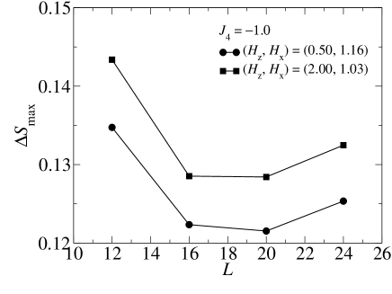
The numerical analysis leading to the nature of the transitions is again based on the behavior of the maximum of the entanglement entropy difference versus the system size. The entropy differences along the transition lines between the F($+x$) and F($\pm z$) show similar behavior as those shown in Fig. 2, therefore they can be viewed as first-order transition lines. On the other hand, the transition lines between the $<$3,1$>$$(\pm)$ and the F($\pm z$) phases can only be analyzed in lattices with periodicity of 4 site spacings. That is, the size $L$ must be a multiple of 4, so as to make the lattice commensurate with the $<$3,1$>$$(\pm)$ orderings. Figure 4 shows the behavior of the maximum of the entanglement entropy difference $\Delta{S_{\max}}$ for $L=12,16,20,$ and $24$. The data were obtained along the transition line in the region $0.0\leq H_{\rm z}\leq 4.0$ of Fig. 3 for two values of the critical fields, $(H_{\rm z},H_{\rm x})$ = $(0.50,1.16)$ and $(2.00,1.03)$. At first, $\Delta{S_{\max}}$ decreases with $L$. Then it passes through a a minimum and rises between $L=20$ and $24$. We believe this trend will continue, so that the transition is of second order. Unfortunately, at present, it is numerically prohibitive to tackle larger lattices, considering that the next relevant size would be $L=28$.

Figure 5: Phase diagram in the ($J_{4}$-$H_{\rm z}$)-plane for the case $H_{\rm x}$=$1.0$. The triangles separate a field-induced ferromagnetic phase with net magnetization in the +$x$ direction, F(+$x$), from two other ferromagnetic phases with magnetizations along the $\pm z$ directions, F(+$z$) and F($-z$). The phases $<$3,1$>$$(+)$ and $<$3,1$>$$(-)$ are separated by a first-order transition line (with stars). For $J_{4}>1$, there is a first-order transition line (with crosses) separating the two field-induced ferromagnetic phases F(+$z$) and F($-z$). The squares are results from finite-size scaling, while the other data are from entanglement entropy.

For completeness we also perform calculations for $H_{\rm x}=1.0$ to investigate the occurrence of phase transitions when the transverse field is kept constant, so that the system is always in the quantum regime. The phase diagram in the ($J_{4}$-$H_{\rm z}$)-plane is shown in Fig. 5. The ferromagnetic phase with net magnetization in the $x$-direction F($+x$) appears as an island surrounded by the $<$3,1$>$$(+)$, $<$3,1$>$$(-)$, F($+z$), and F($-z$) phases.

The transition lines separating the $<$3,1$>$ from the F phases are of second order. The other transition lines are all of first order. Along the boundary line separating the $<$3,1$>$ phases, the ground-states are quantum states containing equal contributions from $<$3,1$>$$(+)$ and $<$3,1$>$$(-)$ configurations, as well as from a background of states induced by the transverse field. On the other side of the diagram for $J_{4}>1.0$, along the transition line between the two F phases, the ground states are formed by the coexistence of ferromagnetic, antiferromagnetic, and $<$2,2$>$ orderings, with additional background states caused by the presence of the transverse magnetic field. Finally, there are four multi-critical points, which are located at ($J_{4}$, $H_{\rm z}$)$=$($-0.84\pm 0.01$, $\pm 0.74\pm 0.01$) and ($\pm 1.0$, $0.0$).

V Conclusions

We have studied the competing effects of a magnetic field with components in the longitudinal and transverse directions on the quantum behavior of an Ising-like chain with four-spin interactions. The entanglement entropy and finite-size scaling methods have been used to obtain the phase diagrams of the system. A rich variety of quantum phases and multi-critical points have been show to be present in the model. Both first and second order transitions are observed among the phases. Under certain conditions the physics of atoms interacting in a one dimensional lattice may be captured by the model Hamiltonian analyzed here. It would be interesting to see how optical lattice techniques could be implemented to simulate the present model.

We thank FAPERJ (Brazilian agency) and PROPPI/UFF for financial support. (O.F.A.B.) acknowledges support from the Murdoch College of Science Research Program and a grant from the Research Corporation through the Cottrell College Science Award No. CC5737.

References

- (1) J. Simon, W.S. Bakr, R. Ma, M.E. Tai, P.M. Preiss, and M. Greiner, Nature (London) 472, 307 (2011).
- (2) D. Jacksch, C. Bruder, J.I. Cirac, C.W. Gardiner, and P. Zoller, Phys. Rev. Lett. 81, 3108 (1998).
- (3) A. Kastberg, W.D. Phillips, S.L. Rolston, R.J.C. Spreeuw, and P.S. Jessen, Phys. Rev. Lett. 74, 1542 (1995); G. Raithel, W.D. Philips, and S.L. Rolston, ibid. 81, 3615 (1998).
- (4) M. Greiner, O. Mandel, T. Esslinger, T.W. Heanch, and I. Bloch, Nature (London) 415, 39 (2002); M. Greiner, O. Mandel, T.W. Heanch, and I. Bloch, ibid 419, 51 (2002).
- (5) O. Mandel, M. Greiner, A. Widera, T. Rom, T.W. Heanch, and I. Bloch, Nature (London) 425, 937 (2003).
- (6) J.K. Pachos and E. Rico, Phys. Rev. A 70, 053620 (2004).
- (7) J.K. Pachos and M.B. Plenio, Phys. Rev. Lett. 93, 056402 (2004).
- (8) C. D’Cruz and J.K. Pachos, Phys. Rev. A 72, 043608 (2005).
- (9) K.A Penson, Phys. Rev. B 29, 2404 (1984).
- (10) O.F. de Alcantara Bonfim and J. Florencio, Phys. Rev. B 74, 134413 (2006).
- (11) O.F. de Alcantara Bonfim, A. Saguia, B. Boechat, and J. Florencio, to be published.
- (12) J.F. McCabe and T. Wydro, Phys. Rev. E 84, 031123 (2011).
- (13) S.L.A. de Queiroz, Phys. Rev. E 84, 031132 (2011).
- (14) L. Turban, J. Phys. C 15, L65 (1982).
- (15) K.A. Penson, R. Jullien, and P. Pfeuty, Phys. Rev. B 26, 6334 (1982).
- (16) J.C. Xavier, F.C. Alcaraz, Phys. Rev. B 84, 094410 (2011).
- (17) S. Nishimoto, Phys. Rev. B 84, 195108 (2011).
- (18) P.R.C. Guimarães, J.A. Plascak, F.C. Sá Barreto, and J. Florencio, Phys. Rev. B 66, 064413 (2002).
- (19) P. Calabrese, J. Cardy, J. Stat. Mech. P06002 (2004).
- (20) M. Barber, Phase Transition and Critical Phenomena, Vol. 8 (Academic Press, New York, 1993).
- (21) E. Dagotto and A. Moreo, Phys. Rev. D 31, 865 (1985); E.R. Gagliano, E. Dagotto, A. Moreo, and F.C. Alcaraz, Phys. Rev. B 34, 1677 (1986).