Proximal Heterogeneous Block Input-Output Method and application to Blind Ptychographic Diffraction Imaging

Abstract

We propose a general alternating minimization algorithm for nonconvex optimization problems with separable structure and nonconvex coupling between blocks of variables. To fix our ideas, we apply the methodology to the problem of blind ptychographic imaging. Compared to other schemes in the literature, our approach differs in two ways: (i) it is posed within a clear mathematical framework with practically verifiable assumptions, and (ii) under the given assumptions, it is provably convergent to critical points. A numerical comparison of our proposed algorithm with the current state-of-the-art on simulated and experimental data validates our approach and points toward directions for further improvement.

Keywords:

Alternating minimization, deconvolution, Kurdyka-Łojasiewicz, nonconvex-nonsmooth minimization, ptychography.

1 Introduction

We consider algorithms for nonconvex constrained optimization problems of the following form

$$\mbox{ Find }\left(\overline{x},\overline{y},\overline{z}\right)\in\operatorname*{arg\,min}\left\{F\left(x,y,z\right)~{}|~{}\left(x,y,z\right)\in C\equiv X\times Y\times Z\right\}.$$ (1.1)

Here $X\times Y\times Z\subset\mathbb{R}^{p}\times\mathbb{R}^{q}\times\mathbb{R}^{r}$ (that is, the constraints apply to disjoint blocks of variables) and $F$ is a nonlinear penalty function characterizing the coupling between the blocks of variables. It will be convenient to reformulate problem (1.1) using indicator functions. The indicator function of a set $C$ is defined as $\iota_{C}\left(x\right)=0$ for $x\in C$ and $\iota_{C}\left(x\right)=+\infty$ for $x\notin C$. Define

$$\Psi\left(x,y,z\right)\equiv F\left(x,y,z\right)+\iota_{X}\left(x\right)+\iota_{Y}\left(y\right)+\iota_{Z}\left(z\right).$$ (1.2)

An equivalent formulation of (1.1) is the formally unconstrained nonsmooth optimization problem

$$\mbox{ Find }\left(\overline{x},\overline{y},\overline{z}\right)\in\operatorname*{arg\,min}_{\left(x,y,z\right)\in\mathbb{R}^{p}\times\mathbb{R}^{q}\times\mathbb{R}^{r}}\left\{\Psi\left(x,y,z\right)\right\}.$$ (1.3)

Algorithms for solving (1.1) or (1.3) typically seek only to satisfy first-order necessary conditions for optimality, and the algorithm we propose below is no different. These conditions are given compactly by

$$0\in\nabla F\left(x^{*},y^{*},z^{*}\right)+\partial\iota_{X}\left(x^{*}\right)+\partial\iota_{Y}\left(y^{*}\right)+\partial\iota_{Z}\left(z^{*}\right),$$ (1.4)

where $\partial f\left(z\right)$ is a set, the subdifferential, that generalizes the notion of a gradient for nonsmooth, subdifferentially regular functions $f$ defined precisely in Definition 3.1 below.

For the sake of fixing the ideas, we focus on the particular application of blind ptychography, however our goal and approach are much more general. The partially smooth character of the objective $\Psi$ in (1.2) is a common feature in many optimization models which involve sums of functions, some of which are smooth and some of which are not. Forward-backward-type algorithms are frequently applied to such models, and our approach is no different. The particular three-block structure of the problem is easily generalized to $M$ blocks. The crucial feature of the model for algorithms, and what we hope to highlight in the present study, is the quantification of continuity of the partial gradients of $F$ with respect only to blocks of variables. This is in contrast to more classical approaches which rely on the continuity of $\nabla F$ with respect to all the variables simultaneously (see [4]). For the ptychography application, such a requirement prohibits a convergence analysis along the lines of [4] since the gradient $\nabla F$ is not Lipschitz continuous. However, the partial gradients with respect to the blocks of variables are Lipschitz continuous. Following [9], this allows us to prove, in Section 3, convergence of the blocked algorithm given below (Algorithm 2.1) to feasible critical points.

Our abstract formulation of the blind ptychography problem can be applied to many different applications including control, machine learning, and deconvolution. We do not attempt to provide a review of the many different approaches to these types of problems, or even a more focused review of numerical methods for ptychography, but rather to provide a common theoretical framework by which a variety of methods can be understood. Our focus on ptychography is due to the success of two algorithms, one by Maiden and Rodenburg [18] and the other due to Thibault and collaborators [24]. These two touchstone methods represent, for us, fundamental computational methods whose structure serves as a central bifurcation in numerical strategies. Moreover, the prevalence of these two methods in practice ensures that our theoretical framework will have the greatest practical impact. (Which is not to say that the methods are the most efficient [19, 23].) We present an algorithmic framework in Section 2 by which these algorithms can be understood and analyzed. We present in Section 3 a theory of convergence of the most general Algorithm 2.1 which is refined with increasingly stringent assumptions until it achieves the form of Algorithm 3.4 that can be immediately applied to ptychography. The specialization of our algorithm to ptychography is presented in Section 4 and summarized in Algorithm 4.1. We compare, in Section 5, Algorithm 4.1 with the state-of-the-art on simulated and experimental data.

2 Algorithms and Modeling

The solution we seek is a triple, $(\overline{x},\overline{y},\overline{z})$ that satisfies a priori constraints, denoted by $C$, as well as a model characterizing the coupling between the variables. We begin naively with a very intuitive idea for solving (1.1): alternating minimization (AM) with respect to the three separate blocks of variables $x$, $y$ and $z$. More precisely, starting with any $\left(x^{0},y^{0},z^{0}\right)\in X\times Y\times Z$, we consider the following algorithm:

$$x^{k+1} \in\operatorname*{arg\,min}_{x\in X}\left\{F\left(x,y^{k},z^{k}\right)\right\},$$ (2.1a)

$$y^{k+1} \in\operatorname*{arg\,min}_{y\in Y}\left\{F\left(x^{k+1},y,z^{k}\right)\right\},$$ (2.1b)

$$z^{k+1} \in\operatorname*{arg\,min}_{z\in Z}\left\{F\left(x^{k+1},y^{k+1},z\right)\right\}.$$ (2.1c)

While the simplicity of the above algorithm is attractive, there are several considerations one must address:

• The convergence results for the AM method are limited and applicable only in the convex setting. It is unknown if the AM method converges in the nonconvex setting. Of course, in the general nonconvex setting we can not expect for convergence to global optimum but even convergence to critical points is not known. In [3] the authors prove convergence to critical points for a regularized variant of alternating minimization. We follow this approach in Algorithm 2.1 below, applying proximal regularization in each of the steps to obtain provable convergence results.

• Each one of the steps of the algorithm involves solving an optimization problem over just one of the blocks of variables. Forward-backward-type methods are common approaches to solving such minimization problems [10], and can be mixed between blocks of variables [9]. Forward operators are typically applied to the ill-posed or otherwise computationally difficult parts of the objective (usually appearing within the smooth part of the objective) while backward operators are applied to the well-posed parts of the objective (appearing often in the nonsmooth part).

In the particular case of ptychography, the subproblems with respect to the $x$ and $y$ variables (steps (2.1a) and (2.1b) of the algorithm) are ill-posed. We handle this by applying a regularized backward operator (the prox operator) to blockwise-linearizations of the ill-posed forward steps. The objective is well-posed, and particularly simple, with respect to the third block of variables, $z$, so we need only employ a backward operator for this step. Generalizing, our approach addresses issue (ii) above by handling each of the blocks of variables differently.

Our presentation of Algorithm 2.1 makes use of the following notation. For any fixed $y\in\mathbb{R}^{q}$ and $z\in\mathbb{R}^{r}$, the function $x\mapsto F\left(x,y,z\right)$ is continuously differentiable and its partial gradient, $\nabla_{x}F\left(x,y,z\right)$, is Lipschitz continuous with moduli $L_{x}\left(y,z\right)$. The same assumption holds for the function $y\mapsto F\left(x,y,z\right)$ when $x\in\mathbb{R}^{p}$ and $z\in\mathbb{R}^{r}$ are fixed. In this case, the Lipschitz moduli is denoted by $L_{y}\left(x,z\right)$. Define $L_{x}^{\prime}\left(y,z\right)\equiv\max\left\{L_{x}\left(y,z\right),\eta_{x}\right\}$ where $\eta_{x}$ is an arbitrary positive number. Similarly define $L_{y}^{\prime}\left(x,z\right)\equiv\max\left\{L_{y}\left(x,z\right),\eta_{y}\right\}$ where $\eta_{y}$ is an arbitrary positive number.

Algorithm 2.1 (Proximal Block Implicit-Explicit Algorithm).

 
Initialization. Choose $\alpha,\beta>1$, $\gamma>0$ and $\left(x^{0},y^{0},z^{0}\right)\in X\times Y\times Z$.
General Step ($k=0,1,\ldots$) 1. Set $\alpha^{k}=\alpha L_{x}^{\prime}\left(y^{k},z^{k}\right)$ and select $$x^{k+1}\in\operatorname*{arg\,min}_{x\in X}\left\{\left\langle{x-x^{k},\nabla_{x}F\left(x^{k},y^{k},z^{k}\right)}\right\rangle+\frac{\alpha^{k}}{2}\left\|{x-x^{k}}\right\|^{2}\right\},$$ (2.2) 2. Set $\beta^{k}=\beta L_{y}^{\prime}\left(x^{k+1},z^{k}\right)$ and select $$y^{k+1}\in\operatorname*{arg\,min}_{y\in Y}\left\{\left\langle{y-y^{k},\nabla_{y}F\left(x^{k+1},y^{k},z^{k}\right)}\right\rangle+\frac{\beta^{k}}{2}\left\|{y-y^{k}}\right\|^{2}\right\},$$ (2.3) 3. Select $$z^{k+1}\in\operatorname*{arg\,min}_{z\in Z}\left\{F\left(x^{k+1},y^{k+1},z\right)+\frac{\gamma}{2}\left\|{z-z^{k}}\right\|^{2}\right\}.$$ (2.4)

The regularization parameters $\alpha^{k}$ and $\beta^{k}$, $k\in\mathbb{N}$, are discussed in Section 5. For the moment, suffice it to say that these parameters are inversely proportional to the stepsize in Steps (2.2) and (2.3) of the algorithm (see Section 3). Noting that $\alpha_{k}$ and $\beta_{k}$, $k\in\mathbb{N}$, are directly proportional to the respective partial Lipschitz moduli, the larger the partial Lipschitz moduli the smaller the stepsize, and hence the slower the algorithm progresses.

This brings to light another advantage of blocking strategies that goes beyond convergence proofs: algorithms that exploit block structures inherent in the objective function achieve better numerical performance by taking heterogeneous step sizes optimized for the separate blocks. There is, however, a price to be paid in the blocking strategies that we explore here: namely, they result in procedures that pass sequentially between operations on the blocks, and as such are not immediately parallelizable. Here too, the ptychography application generously rewards us with added structure, as we show in Section 3.3, permitting parallel computations on highly segmented blocks.

The convergence theory developed in Section 3 is independent of the precise form of the coupling function $F$ and independent of the precise form of the constraints. For our analysis we require that $F$ is differentiable with $\nabla F$ Lipschitz continuous on bounded domains, and the partial gradient $\nabla_{x}F$ (globally) Lipschitz continuous as a mapping on $X$ for each $\left(y,z\right)\in Y\times Z$ fixed, and partial gradient $\nabla_{y}F$ (globally) Lipschitz continuous as a mapping on $Y$ for $\left(x,z\right)\in X\times Z$ fixed. The constraint sets $X$, $Y$ and $Z$ could be very general, we only assume that they are closed and disjoint. This is discussed more precisely below. The analysis presented in Section 3 guarantees only that Algorithm 2.1 converges to a point satisfying (1.4), which, it is worth reiterating, are not necessarily solutions to (1.1).

2.1 Blind Ptychography

In scanning ptychography, an unknown specimen is illuminated by a localized electromagnetic beam and the resulting wave is recorded on a CCD array somewhere downstream along the axis of propagation of the wave (i.e., in the far field or the near field of the object). A ptychographic dataset consists of a series of such observations, each differing from the others by a spatial shift of either the object or the illumination. In the original ptychographic reconstruction procedure [13] it was assumed that the illuminating beam was known. What we call blind ptychography, in analogy with blind deconvolution, reflects the fact that the beam is not completely known, this corresponds to what is commonly understood by ptychography in modern applications [21, 22, 18, 24]. Here the problem is to simultaneously reconstruct the specimen and illuminating beam from a given ptychgraphic dataset. We will treat the case of scanning x-ray ptychography with far field measurements. This is not exhaustive of all the different settings one might encounter, but the mathematical structure of the problem, our principal interest, is qualitatively the same for all cases. For a review of ptychothographic methods, see [1] and the reference herein.

We formulate the ptychography problem on the product space $\mathbb{C}^{n}\times\mathbb{C}^{n}\times\mathbb{C}^{n\times m}$ where the first block $\mathbb{C}^{n}$ corresponds to the model space for the probe, the second block corresponds to the model space for the specimen, and the third block corresponds to the model space for the data/observations. The physical model space equipped with the real inner product is isomorphic to the Euclidean space $\left(\mathbb{R}^{2}\right)^{n}\times\left(\mathbb{R}^{2}\right)^{n}\times\left(\mathbb{R}^{2}\right)^{n\times m}$ with the inner product $\left\langle{\left(x,y,z\right),\left(x^{\prime},y^{\prime},z^{\prime}\right)}\right\rangle\equiv\sum_{j=1}^{n}\left\langle{x_{j},x^{\prime}_{j}}\right\rangle+\sum_{j=1}^{n}\left\langle{y_{j},y^{\prime}_{j}}\right\rangle+\sum_{j=1}^{n}\sum_{i=1}^{m}\left\langle{z_{ij},z^{\prime}_{ij}}\right\rangle$ for $x_{i},y_{i},z_{ij}\in\mathbb{R}^{2}$. This is in fact how complex numbers are represented on a computer, and hence the model space $\mathbb{C}^{n}$ with real inner product is just an efficient shorthand for $\left(\mathbb{R}^{2}\right)^{n}$ with the standard inner product for such product spaces. We will therefore retain the complex model space with real inner product when describing this problem, noting that all linear operators on this space have analogues on the space $\left(\mathbb{R}^{2}\right)^{n}$. The theory, however, will be set on real finite dimensional vector spaces.

Denote ${\bf z}\equiv\left(z_{1},z_{2},\ldots,z_{m}\right)$ with $z_{j}\in\mathbb{C}^{n}$ ($j=1,2,\ldots,m$). The objective function in our general optimization problem (1.1), $F:\mathbb{C}^{n}\times\mathbb{C}^{n}\times\mathbb{C}^{n\times m}\rightarrow\mathbb{R}_{+}$, is given by

$$F\left(x,y,{\bf z}\right)\equiv\sum_{j=1}^{m}\left\|{S_{j}\left(x\right)\odot y-z_{j}}\right\|^{2}.$$ (2.5)

Here $S_{j}:\mathbb{C}^{n}\to\mathbb{C}^{n}$ denotes $j$-th shift operator which shifts the indexes in $x\in\mathbb{C}^{n}$ in some prescribed fashion and $\odot$ is the elementwise Haadamard product. This function measures in some sense the distance to the set

$$\mathcal{M}\equiv\left\{\left(x,y,{\bf z}\right)\in\mathbb{C}^{n}\times\mathbb{C}^{n}\times\mathbb{C}^{n\times m}~{}|~{}S_{j}\left(x\right)\odot y=z_{j},\,\,j=1,2,\ldots,m\right\}.$$ (2.6)

Let $b_{j}\in\mathbb{R}^{n}$, $j=1,2,\ldots,m$, denote the experimental observations, and $\mathcal{F}$ be a $2$D discrete Fourier transform (of dimension $\sqrt{n}\times\sqrt{n}$) rearranged for vectors on $\mathbb{C}^{n}$. The constraints $X$, $Y$, and $Z$ are separable and given by

$$X \equiv\{\mbox{qualitative constraints on the probe}\},$$ (2.7a)

$$Y \equiv\{\mbox{qualitative constraints on the specimen}\},$$ (2.7b)

$$Z \equiv Z_{1}\times Z_{2}\times\cdots\times Z_{m},$$

$$\mbox{where }Z_{j}\equiv\left\{z\in\mathbb{C}^{n}~{}|~{}\left|\left(\mathcal{F}z\right)_{l}\right|=b_{jl},\;(l=1,2,\ldots,n)\right\}\quad(j=1,2,\ldots,m).$$ (2.7c)

The qualitative constraints characterized by $X$ and $Y$ are typically a mixture of support, support-nonnegativity or magnitude constraints corresponding respectively to whether the illumination and specimen are supported on a bounded set, whether these (most likely only the specimen) are “real objects” that somehow absorb or attenuate the probe energy, or whether these are “phase” objects with a prescribed intensity but varying phase. A support constraint for the set $X$, for instance, would be represented by

$$X\equiv\left\{x=(x_{1},x_{2},\dots,x_{n})\in\mathbb{C}^{n}~{}|~{}|x_{i}|\leq R~{}(i=1,2,\dots,n)\mbox{ and, for }i\notin\mathbb{I}_{X},~{}x_{i}=0\right\},$$ (2.8)

where $\mathbb{I}_{X}$ is the index set corresponding to which pixels in the field of view the probe beam illuminates and $R$ is some given amplitude. A mixture of support and amplitude constraints for the set $Y$ would be represented by

$$Y\equiv\left\{y=(y_{1},y_{2},\dots,y_{n})\in\mathbb{C}^{n}~{}|~{}0\leq\underline{\eta}\leq\left|y_{i}\right|\leq\overline{\eta}\mbox{ and, for }i\notin\mathbb{I}_{Y},y_{i}=0\right\},$$ (2.9)

where the index set $\mathbb{I}_{Y}$ is the analogous index set for the support of the specimen, and $\underline{\eta}/\overline{\eta}$ are lower/upper bounds on the intensity of the specimen. The set $Z$ is nothing more than the phase set appearing in feasibility formulations of the phase retrieval problem [16].

Remark 2.1 (Feasibility versus minmization).

Since the algorithms discussed below involve, at some point, projections onto these sets, it is worthwhile noting here that, while, in most applications, the projections onto the sets $X$, $Y$ and $Z$ have a closed form and can be computed very accurately and efficiently, we are unaware of any method, analytic or otherwise, for computing the projection onto the set $\mathcal{M}$ defined by (2.6). For this reason, we have avoided formulation of the problem as a (nonconvex) feasibility problem

$$\mbox{Find }\overline{x}\in\mathcal{M}\cap\left(X\times Y\times Z\right).$$

Nevertheless, this essentially two-set feasibility model suggests a wide range of techniques within the family of projection methods, alternating projections, averaged projections and Douglas–Rachford being representative members. In contrast to these, our approach is essentially a forward-backward method that avoids the difficulty of computing a projection onto the set $\mathcal{M}$ by instead minimizing a nonnegative coupling function $F$ that takes the value $0$ (only) on $\mathcal{M}$.

3 Algorithm Analysis

3.1 Mathematical Preliminaries

Algorithm 2.1 consists of three steps all of which reduce to the computation of a projection onto a given constraint set (convex and nonconvex). Recall that the projection onto a nonempty and closed subset $\Omega$ of a Euclidean space $\mathbb{R}^{d}$, is the (set-valued) mapping $P_{\Omega}:\mathbb{R}^{d}\rightrightarrows\Omega$ defined by

$$P_{\Omega}\left(v\right)\equiv\operatorname*{arg\,min}\left\{\left\|{u-v}\right\|~{}|~{}u\in\Omega\right\}.$$ (3.1)

In Euclidean spaces the projection is single valued if and only if $\Omega$ is convex (in addition to being nonempty and closed). Specializing to the present application, for the constraints specified by (2.7), $P_{C}=\left(P_{X},P_{Y},P_{Z}\right)$ where $P_{X}$, $P_{Y}$ and $P_{Z}$ are, in general, multivalued (consider $P_{C}\left(0\right)$).

Since we are dealing with nonsmooth and nonconvex functions that can take the value $+\infty$, we require the following generalization of the derivative for nonconvex functions.

Definition 3.1 (Subdifferential [20]).

Let $f:\mathbb{R}^{d}\rightarrow\left(-\infty,+\infty\right]$ be proper (not everywhere infinite) and lower semicontinuous (lsc).

• The regular or Fréchet subdifferential of $f$ at $u\in\mathrm{dom}\,{f}$, denoted $\widehat{\partial}f(u)$, is the set of vectors $v\in\mathbb{R}^{d}$ which satisfy

  $$\liminf_{\stackrel{{\scriptstyle w\neq u}}{{w\rightarrow u}}}\frac{f\left(w\right)-f\left(u\right)-\left\langle{v,w-u}\right\rangle}{\left\|{w-u}\right\|}\geq 0.$$ (3.2)

  If $u\notin\mathrm{dom}\,{f}$ then $\widehat{\partial}f\left(u\right)\equiv\emptyset$.

• The limiting subdifferential of $f$ at $u\in\mathrm{dom}\,{f}$, denoted $\partial f\left(u\right)$, is the set of limits of limiting subdifferentials:

  $$\partial f\left(u\right)\equiv\left\{v\in\mathbb{R}^{d}~{}|~{}\exists u^{k}\rightarrow u\mbox{ with }f\left(u^{k}\right)\rightarrow f\left(u\right)\mbox{ and }v^{k}\rightarrow v\mbox{ with }v^{k}\in\widehat{\partial}f\left(u^{k}\right)\mbox{ as }k\rightarrow\infty\right\}.$$

We say that $f$ is subdifferentially regular at $u$ if $\partial f\left(u\right)=\widehat{\partial}f\left(u\right)$, and subdifferentially regular (without reference to the point $u$) if it is subdifferentially regular at every point in $\mathrm{dom}\,{f}$.

The notion of regularity of a set can be understood in terms of the subdifferential regularity of the indicator function of that set. We will call a set Clarke regular if the corresponding indicator function is subdifferentially regular (see [20, Definition 6.4]).

In [9], Bolte et al. present a general procedure for determining convergence to critical points of generic algorithms for nonsmooth and nonconvex problems. The procedure consists of verifying three criteria, two of which are quite standard and shared by most descent algorithms, see e.g., [4]. The third criterion depends not on the algorithm but on the objective function: it must satisfy the Kurdyka-Łojasiewicz (KL) property (see [7, 8] and the references therein).

Definition 3.2 (Kurdyka-Łojasiewicz property).

Let $f:\mathbb{R}^{d}\rightarrow\left(-\infty,+\infty\right]$ be proper and lower semicontinuous. For $\eta\in\left(0,+\infty\right]$ define

$$\mathcal{C}_{\eta}\equiv\left\{\varphi\in C\left[\left[0,\eta\right),\mathbb{R}_{+}\right]\mbox{ such that }\left.\begin{cases}\varphi\left(0\right)=0&\\ \varphi\in C^{1}&\mbox{ on }\left(0,\eta\right)\\ \varphi^{\prime}\left(s\right)>0&\mbox{ for all }s\in\left(0,\eta\right)\end{cases}\right\}\right\}.$$ (3.3)

The function $f$ is said to have the Kurdyka-Łojasiewicz (KL) property at $\overline{u}\in\mathrm{dom}\,{\partial}f$ if there exist $\eta\in\left(0,+\infty\right]$, a neighborhood $U$ of $\overline{u}$ and a function $\varphi\in\mathcal{C}_{\eta}$, such that, for all

$$u\in U\cap[f(\overline{u})<f(u)<f(\overline{u})+\eta],$$

the following inequality holds

$$\varphi\left(f\left(u\right)-f\left(\overline{u}\right)\right)\mathrm{dist}\left(0,\partial f\left(u\right)\right)\geq 1.$$ (3.4)

If $f$ satisfies property (3.4) at each point of $\mathrm{dom}\,{\partial}f$, then $f$ is called a KL function.

For a given function, the KL property can be verified indirectly by checking membership to certain classes of functions, in particular the class of semi-algebraic functions [7]. For the convenience of the reader, we recall here the definition of semi-algebraic functions.

Definition 3.3 (Semi-algebraic sets and functions).

• A $S\subseteq\mathbb{R}^{d}$ is (real) semi-algebraic if there exists a finite number of real polynomial functions $p_{ij},q_{ij}:\mathbb{R}^{d}\rightarrow\mathbb{R}$ such that

  $$S=\bigcup_{j=1}^{N}\bigcap_{i=1}^{K}\left\{u\in\mathbb{R}^{d}:\;p_{ij}\left(u\right)=0\,\text{ and }\,q_{ij}\left(u\right)<0\right\}.$$

• A function $f:\mathbb{R}^{d}\rightarrow\left(-\infty,+\infty\right]$ is semi- algebraic if its graph

  $$\left\{\left(u,t\right)\in\mathbb{R}^{d+1}~{}|~{}f\left(u\right)=t\right\},$$

  is a semi-algebraic subset of $\mathbb{R}^{d+1}$.

The class of semi-algebraic sets is stable under the following operations: finite unions, finite intersections, complementation and Cartesian products. For a thorough catalog of semi-algebraic functions and sets see [2, 3, 4, 9] and the references therein.

While it may not be obvious how directly to verify the KL property it is easy to determine whether a function is semi-algebraic. The remarkable fact about semi-algebraic functions is that, as long as they are lower semi-continuous, they automatically satisfy the KL property on their domain as stated in the following result.

Theorem 3.1 ([7, Th. 3.3, pg. 1215]).

Let $f:\mathbb{R}^{d}\rightarrow\left(-\infty,+\infty\right]$ be a proper lower semicontinuous function. If $f$ is semi-algebraic then it satisfies the KL property at any point in $\mathrm{dom}\,{f}$.

We now show that the ptychography problem, and hence the phase retrieval problem, is semi-algebraic, i.e., both the objective function $F$ and the constraint set $C$ are semi-algebraic.

Proposition 3.2 (Blind ptychography and phase retrieval are semi-algebraic).

The objective function $F$, defined by (2.5), is continuous and semi-algebraic. The constraint sets $X$, $Y$ and $Z$, defined by (2.7), are nonempty, closed and semi-algebraic. Consequently, the corresponding function $\Psi$, defined by (1.2), is a KL function on $X\times Y\times Z$.

Proof sketch.

The physical model is formulated with complex-valued vectors, but $\mathbb{C}^{n}$ with the real inner product is isomorphic to the Euclidean space $\left(\mathbb{R}^{2}\right)^{n}$ with the inner product $\left\langle{x,x^{\prime}}\right\rangle\equiv\sum_{i=1}^{n}\left(x_{i},x^{\prime}_{i}\right)$ for $x_{i},x^{\prime}_{i}\in\mathbb{R}^{2}$. The function $F$ defined by (2.5) is finite everywhere, continuous (indeed, differentiable), and the level sets of the objective $F$ are quadratics with respect to $y$ and $z_{j}$, and quadratic with respect to $x$ under linear transformations. Thus $F$ is semi-algebraic. The sets $X$ and $Y$ are either subspaces (support constraint only, (2.8)) or the intersection of a subspace with a box or ball (support and nonnegativity or support and amplitude constraints (2.9)), and so both of these are nonempty semi-algebraic. The set $Z$ is equivalent to an amplitude constraint in the image space of the linear mapping $\mathcal{F}$ with respect to the 1-norm on each two-dimensional component of the product space $\left(\mathbb{R}^{2}\right)^{n}$. Thus $Z$ is also nonempty semi-algebraic. That $\Psi$ defined by (1.2) is then a KL-function for these $F$, $X$, $Y$, and $Z$ then follows from Theorem 3.1. ∎

3.2 Convergence Analysis

Our convergence analysis is centered on Theorem 3.7, a general result concerning the application of Algorithm 2.1 to problem (1.4). The specialization to the ptychography problem, Proposition 4.1, is then easily achieved by verifying that the assumptions of a refinement, Theorem 3.10, are satisfied. Following [9], we carry out the three-step procedure, outlined in Section 3.1, for proving convergence of the sequence $\left\{\left(x^{k},y^{k},z^{k}\right)\right\}_{k\in\mathbb{N}}$, generated by Algorithm 2.1, to a point satisfying (1.4) provided that the initial point $\left(x^{0},y^{0},z^{0}\right)\in X\times Y\times Z$. The analysis rests on the following assumptions, collected here to avoid repetition.

Assumption 1.

Let $\left\{\left(x^{k},y^{k},z^{k}\right)\right\}_{k\in\mathbb{N}}$ be iterates of Algorithm 2.1 for $\left(x^{0},y^{0},z^{0}\right)\in X\times Y\times Z$. (i) $X\subset\mathbb{R}^{p}$, $Y\subset\mathbb{R}^{q}$, and $Z\subset\mathbb{R}^{r}$ are nonempty and closed. (ii) $F:\mathbb{R}^{p}\times\mathbb{R}^{q}\times\mathbb{R}^{r}\rightarrow\mathbb{R}$ is differentiable on $X\times Y\times Z$ and $\inf F>-\infty$. Moreover, $\nabla_{x}F$ and $\nabla_{y}F$ (as defined above) are Lipschitz continuous with moduli $L_{x}\left(y,z\right)$ and $L_{y}\left(x,z\right)$, respectively. (iii) The gradient of $F$, $\nabla F$, is Lipschitz continuous on bounded domains in $X\times Y\times Z$. Moreover, there exists $\lambda_{x}^{+},\lambda_{y}^{+}>0$ such that $$\sup\left\{L_{x}\left(y^{k},z^{k}\right)~{}|~{}k\in\mathbb{N}\right\}\leq\lambda_{x}^{+}\quad\mbox{ and }\quad\sup\left\{L_{y}\left(x^{k+1},z^{k}\right)~{}|~{}k\in\mathbb{N}\right\}\leq\lambda_{y}^{+}.$$ (3.5) (iv) The iterates $\left\{\left(x^{k},y^{k},z^{k}\right)\right\}_{k\in\mathbb{N}}$ are bounded. (v) The function $\Psi$ defined by (1.2) is a KL function (see Definition 3.2).

Remark 3.1.

In Section 4, we will show that our ptychography model (described in Section 2.1) satisfies these assumptions. For the general setting we point out the following.

1. Boundedness of the iterates Assumption 1(iv)) is a strong assumption that can be handled by a more technical treatment than we would like to present here. For our purposes this can be guaranteed by the physically natural assumption that the constraint set is bounded. Since Algorithm 2.1 is a feasible point algorithm, all iterates belong to the bounded feasible set, hence, in this case, the iterates are bounded.

2. Combining Assumptions 1(ii) and (iii) do not guarantee that the gradient $\nabla F$ is globally Lipschitz, as is the case in the application described below (see Section 4). The inequalities in (3.5) could be obtained in several scenarios, for example, when $F$ is $C^{2}$ and using the boundedness assumption Assumption 1(iv).

We begin with a technical lemma.

Lemma 3.3 (Sufficient decrease property).

Let $h:\mathbb{R}^{d}\rightarrow\mathbb{R}$ be a continuously differentiable function with gradient $\nabla h$ assumed to be $L_{h}$-Lipschitz continuous and let $\Omega$ be a nonempty and closed subset of $\mathbb{R}^{d}$. Fix any $t>L_{h}$. Then, for any $u\in\Omega$ and for $u^{+}\in\mathbb{R}^{d}$ defined by

$$u^{+}\in P_{\Omega}\left(u-\frac{1}{t}\nabla h\left(u\right)\right),$$

we have

$$h\left(u^{+}\right)\leq h\left(u\right)-\frac{1}{2}\left(t-L_{h}\right)\left\|{u^{+}-u}\right\|^{2}.$$

Proof.

The result follows from [9, Lemma 2] where the nonsmooth function $\sigma$ is the indicator function $\iota_{\Omega}$ of the nonempty closed set $\Omega$. ∎

Remark 3.2.

When $\Omega$ is also convex, the conclusion of Lemma 3.3 can be improved (see [6, Lemma 2.3]) to the following

$$h\left(u^{+}\right)\leq h\left(u\right)-\left(t-\frac{L_{h}}{2}\right)\left\|{u^{+}-u}\right\|^{2}.$$

This means that $t>L_{h}/2$ (rather than only $t>L_{h}$, as in the nonconvex case) is enough to guarantee decrease of function value after projected-gradient step.

Using Lemma 3.3 we can prove the following basic property of Algorithm 2.1.

Proposition 3.4 (Sufficient decrease).

Let $\left\{\left(x^{k},y^{k},z^{k}\right)\right\}_{k\in\mathbb{N}}$ be a sequence generated by Algorithm 2.1 for some initial point $\left(x^{0},y^{0},z^{0}\right)\in X\times Y\times Z$. Suppose that conditions (i)-(ii) of Assumption 1 hold. Then the sequence $\left\{F\left(x^{k},y^{k},z^{k}\right)\right\}_{k\in\mathbb{N}}$ is decreasing and

$$\sum_{k=1}^{\infty}\left\|{\left(x^{k+1},y^{k+1},z^{k+1}\right)-\left(x^{k},y^{k},z^{k}\right)}\right\|^{2}<\infty.$$

Hence the sequence $\left\{F\left(x^{k},y^{k},z^{k}\right)\right\}_{k\in\mathbb{N}}$ converges to some $F^{\ast}>-\infty$ as $k\rightarrow\infty$.

Proof.

We apply Lemma 3.3 to the first subproblem (see (2.2)) as follows. Take $h\left(\cdot\right)=F\left(\cdot,y^{k},z^{k}\right)$, $\Omega=X$ and $t=\alpha^{k}>L_{x}^{\prime}\left(y^{k},z^{k}\right)$ to obtain that

$$F\left(x^{k+1},y^{k},z^{k}\right) \leq F\left(x^{k},y^{k},z^{k}\right)-\frac{1}{2}\left(\alpha^{k}-L_{x}\left(y^{k},z^{k}\right)\right)\left\|{x^{k+1}-x^{k}}\right\|^{2}$$

$$\leq F\left(x^{k},y^{k},z^{k}\right)-\frac{1}{2}\left(\alpha^{k}-L_{x}^{\prime}\left(y^{k},z^{k}\right)\right)\left\|{x^{k+1}-x^{k}}\right\|^{2}$$

$$=F\left(x^{k},y^{k},z^{k}\right)-\frac{1}{2}\left(\alpha-1\right)L_{x}^{\prime}\left(y^{k},z^{k}\right)\left\|{x^{k+1}-x^{k}}\right\|^{2}$$

$$\leq F\left(x^{k},y^{k},z^{k}\right)-\frac{1}{2}\left(\alpha-1\right)\eta_{x}\left\|{x^{k+1}-x^{k}}\right\|^{2},$$

where the second inequality follows from the fact that $L_{x}\left(y^{k},z^{k}\right)\leq L_{x}^{\prime}\left(y^{k},z^{k}\right)$ and the last inequality follows from the fact that $\eta_{x}\leq L_{x}^{\prime}\left(y^{k},z^{k}\right)$ and $\alpha>1$. Similarly, applying Lemma 3.3 to the second subproblem (see (2.3)) with $h\left(\cdot\right)=F\left(x^{k+1},\cdot,z^{k}\right)$, $\Omega=Y$ and $t=\beta^{k}>L_{y}^{\prime}\left(x^{k+1},z^{k}\right)$ yields

$$F\left(x^{k+1},y^{k+1},z^{k}\right)\leq F\left(x^{k+1},y^{k},z^{k}\right)-\frac{1}{2}\left(\beta-1\right)\eta_{y}\left\|{y^{k+1}-y^{k}}\right\|^{2}.$$

On the other hand, immediately from the third updating rule (see (2.4)) we get that

$$F\left(x^{k+1},y^{k+1},z^{k+1}\right)\leq F\left(x^{k+1},y^{k+1},z^{k}\right)-\frac{\gamma}{2}\left\|{z^{k+1}-z^{k}}\right\|^{2}.$$

Summing up all these inequalities yields

$$F\left(x^{k+1},y^{k+1},z^{k+1}\right) \leq F\left(x^{k},y^{k},z^{k}\right)-\frac{1}{2}\left(\alpha-1\right)\eta_{x}\left\|{x^{k+1}-x^{k}}\right\|^{2}-\frac{1}{2}\left(\beta-1\right)\eta_{y}\left\|{y^{k+1}-y^{k}}\right\|^{2}$$

$$-\frac{\gamma}{2}\left\|{z^{k+1}-z^{k}}\right\|^{2}.$$

Denote $\lambda^{-}\equiv\left(1/2\right)\min\left\{\left(\alpha-1\right)\eta_{x},\left(\beta-1\right)\eta_{y},\gamma\right\}$. Thus

$$F\left(x^{k+1},y^{k+1},z^{k+1}\right)\leq F\left(x^{k},y^{k},z^{k}\right)-\lambda^{-}\left\|{\left(x^{k+1},y^{k+1},z^{k+1}\right)-\left(x^{k},y^{k},z^{k}\right)}\right\|^{2}.$$ (3.6)

This proves that the sequence $\left\{F\left(x^{k},y^{k},z^{k}\right)\right\}_{k\in\mathbb{N}}$ is decreasing. Since, in addition, we know that $F$ is bounded from below (see Assumption 1(ii)), we thus have a decreasing sequence on a compact interval and it follows that $\left\{F\left(x^{k},y^{k},z^{k}\right)\right\}_{k\in\mathbb{N}}$ converges to some $F^{\ast}>-\infty$. Summing up this inequality, for $k=1,2,\ldots,N$, yields

$$\sum_{k=1}^{N}\left\|{\left(x^{k+1},y^{k+1},z^{k+1}\right)-\left(x^{k},y^{k},z^{k}\right)}\right\|^{2} \leq\frac{1}{\lambda^{-}}\left(F\left(x^{1},y^{1},z^{1}\right)-F\left(x^{N+1},y^{N+1},z^{N+1}\right)\right)$$

$$\leq\frac{F\left(x^{1},y^{1},z^{1}\right)-F^{\ast}}{\lambda^{-}},$$ (3.7)

where the last inequality holds true since $F\left(x^{N+1},y^{N+1},z^{N+1}\right)\geq F^{\ast}$. Taking the limit as $N\rightarrow\infty$ yields boundedness of the sum of step-lengths and completes the proof. ∎

Before proving the second step, we obtain the following immediate consequence.

Corollary 3.5 (Rate of asymptotic regularity).

Let $\left\{\left(x^{k},y^{k},z^{k}\right)\right\}_{k\in\mathbb{N}}$ be a sequence generated by Algorithm 2.1 for some initial point $\left(x^{0},y^{0},z^{0}\right)\in X\times Y\times Z$ and define the corresponding sequence of steps $\left\{s^{k}\right\}_{k\in\mathbb{N}\setminus\{0\}}$ by $s^{k+1}\equiv\left(x^{k+1},y^{k+1},z^{k+1}\right)-\left(x^{k},y^{k},z^{k}\right)$. Suppose that conditions (i)-(ii) of Assumption 1 hold. Then $s^{k}\rightarrow 0$ as $k\rightarrow\infty$ with the following rate

$$\min_{k=1,2,\ldots,N}\left\|{s^{k+1}}\right\|\leq\sqrt{\frac{F\left(x^{1},y^{1},z^{1}\right)-F^{\ast}}{N\lambda^{-}}},$$

where $\lambda^{-}\equiv\left(1/2\right)\min\left\{\left(\alpha-1\right)\eta_{x},\left(\beta-1\right)\eta_{y},\gamma\right\}$ and $F^{\ast}\equiv\lim_{k\rightarrow\infty}F\left(x^{k},y^{k},z^{k}\right)$.

Proof.

From (3.7) we obtain that

$$N\min_{k=1,2,\ldots,N}\left\|{s^{k+1}}\right\|^{2}\leq\sum_{k=1}^{N}\left\|{s^{k+1}}\right\|^{2}\leq\frac{F\left(x^{1},y^{1},z^{1}\right)-F^{\ast}}{\lambda^{-}},$$

and thus

$$\min_{k=1,2,\ldots,N}\left\|{s^{k+1}}\right\|^{2}\leq\frac{F\left(x^{1},y^{1},z^{1}\right)-F^{\ast}}{N\lambda^{-}}.$$

The result now easily follows. ∎

Proposition 3.6 (Lipschitz paths).

Let $\left\{(x^{k},y^{k},z^{k})\right\}_{k\in\mathbb{N}}$ be a sequence generated by Algorithm 2.1 for some initial point $\left(x^{0},y^{0},z^{0}\right)\in X\times Y\times Z$. Suppose that conditions (i)-(iv) of Assumption 1 hold. For each positive integer $k$, define the following three quantities: $A_{z}^{k}\equiv\gamma\left(z^{k-1}-z^{k}\right)$,

$$A_{x}^{k}\equiv\alpha^{k-1}\left(x^{k-1}-x^{k}\right)+\nabla_{x}F\left(x^{k},y^{k},z^{k}\right)-\nabla_{x}F\left(x^{k-1},y^{k-1},z^{k-1}\right),$$

and

$$A_{y}^{k}\equiv\beta^{k-1}\left(y^{k-1}-y^{k}\right)+\nabla_{y}F\left(x^{k},y^{k},z^{k}\right)-\nabla_{y}F\left(x^{k},y^{k-1},z^{k-1}\right).$$

Then $A^{k}\equiv\left(A_{x}^{k},A_{y}^{k},A_{z}^{k}\right)\in\partial\Psi\left(x^{k},y^{k},z^{k}\right)$ and there exists $\delta>0$ such that

$$\left\|{A^{k}}\right\|\leq\left(3\lambda^{+}+2\delta\right)\left\|{\left(x^{k},y^{k},z^{k}\right)-\left(x^{k-1},y^{k-1},z^{k-1}\right)}\right\|,$$

where $\lambda^{+}\equiv\max\left\{\lambda_{x}^{+},\lambda_{y}^{+},\gamma\right\}$

Proof.

Let $k$ be a positive integer. Writing the optimality condition of the first updating rule yields

$$\nabla_{x}F\left(x^{k-1},y^{k-1},z^{k-1}\right)+\alpha^{k-1}\left(x^{k}-x^{k-1}\right)+w_{x}^{k}=0,$$

where $w_{x}^{k}\in\partial\iota_{X}\left(x^{k}\right)$. Hence

$$\nabla_{x}F\left(x^{k-1},y^{k-1},z^{k-1}\right)+w_{x}^{k}=\alpha^{k-1}\left(x^{k-1}-x^{k}\right).$$

It is clear from the definition of $\Psi$ (see (1.2)), that

$$\partial_{x}\Psi\left(x^{k},y^{k},z^{k}\right)=\nabla_{x}F\left(x^{k},y^{k},z^{k}\right)+\partial\iota_{X}\left(x^{k}\right).$$

Combining these two facts proves that $A_{x}^{k}\in\partial_{x}\Psi\left(x^{k},y^{k},z^{k}\right)$. Following the same arguments applied on the second updating rule yields the desired result that $A_{y}^{k}\in\partial_{y}\Psi\left(x^{k},y^{k},z^{k}\right)$. Now, writing the optimality condition of the third updating rule yields

$$\nabla_{z}F\left(x^{k},y^{k},z^{k}\right)+\gamma\left(z^{k}-z^{k-1}\right)+w_{z}^{k}=0,$$

for $w_{z}^{k}\in\partial\iota_{Z}\left(z^{k}\right)$, hence $A_{z}^{k}\in\partial_{z}\Psi\left(x^{k},y^{k},z^{k}\right)$.

We begin with an estimation of the norm of $A_{x}^{k}$. From Assumption  1(iii) and (iv), there exists $\delta>0$ such that

$$\left\|{\nabla_{x}F\left(x^{k},y^{k},z^{k}\right)-\nabla_{x}F\left(x^{k-1},y^{k-1},z^{k-1}\right)}\right\| \leq\left\|{\nabla F\left(x^{k},y^{k},z^{k}\right)-\nabla F\left(x^{k-1},y^{k-1},z^{k-1}\right)}\right\|$$

$$\leq\delta\left\|{\left(x^{k},y^{k},z^{k}\right)-\left(x^{k-1},y^{k-1},z^{k-1}\right)}\right\|.$$

Thus, from the definition of $\lambda^{+}$ we obtain

$$\left\|{A_{x}^{k}}\right\| \leq\alpha^{k-1}\left\|{x^{k-1}-x^{k}}\right\|+\left\|{\nabla_{x}F\left(x^{k},y^{k},z^{k}\right)-\nabla_{x}F\left(x^{k-1},y^{k-1},z^{k-1}\right)}\right\|$$

$$\leq\lambda_{x}^{+}\left\|{x^{k-1}-x^{k}}\right\|+\delta\left\|{\left(x^{k},y^{k},z^{k}\right)-\left(x^{k-1},y^{k-1},z^{k-1}\right)}\right\|$$

$$\leq\left(\lambda_{x}^{+}+\delta\right)\left\|{\left(x^{k},y^{k},z^{k}\right)-\left(x^{k-1},y^{k-1},z^{k-1}\right)}\right\|,$$

where the second inequality follows from Assumption 1(iii). A similar argument yields

$$\left\|{A_{y}^{k}}\right\|\leq\left(\lambda_{y}^{+}+\delta\right)\left\|{\left(x^{k},y^{k},z^{k}\right)-\left(x^{k-1},y^{k-1},z^{k-1}\right)}\right\|.$$

Thus

$$\left\|{A^{k}}\right\| \leq\left\|{A_{x}^{k}}\right\|+\left\|{A_{y}^{k}}\right\|+\left\|{A_{z}^{k}}\right\|\leq\left(\lambda_{x}^{+}+\lambda_{y}^{+}+2\delta\right)\left\|{\left(x^{k},y^{k},z^{k}\right)-\left(x^{k-1},y^{k-1},z^{k-1}\right)}\right\|+\gamma\left\|{z^{k-1}-z^{k}}\right\|$$

$$\leq\left(3\lambda^{+}+2\delta\right)\left\|{\left(x^{k},y^{k},z^{k}\right)-\left(x^{k-1},y^{k-1},z^{k-1}\right)}\right\|.$$

This proves the desired result. ∎

We are now ready to prove the main result of this section, namely convergence of Algorithm 2.1 to points satisfying (1.4) for any initial point $\left(x^{0},y^{0},z^{0}\right)\in X\times Y\times Z$. It is in deducing the last step of the general case that we use the assumption that $\Psi$ satisfies the KL inequality (3.4).

Theorem 3.7 (Convergence to critical points).

Let $\left\{\left(x^{k},y^{k},z^{k}\right)\right\}_{k\in\mathbb{N}}$ be a sequence generated by Algorithm 2.1 for some initial point $\left(x^{0},y^{0},z^{0}\right)\in X\times Y\times Z$. Suppose that Assumption 1 holds. Then following assertions hold.

1. The sequence $\left\{\left(x^{k},y^{k},z^{k}\right)\right\}_{k\in\mathbb{N}}$ has finite length, that is,

   $$\sum_{k=1}^{\infty}\left\|{\left(x^{k+1},y^{k+1},z^{k+1}\right)-\left(x^{k},y^{k},z^{k}\right)}\right\|<\infty.$$

2. The sequence $\left\{\left(x^{k},y^{k},z^{k}\right)\right\}_{k\in\mathbb{N}}$ converges to a point $\left(x^{\ast},y^{\ast},z^{\ast}\right)$ satisfying (1.4).

Proof.

The result follows from Propositions 3.4 and 3.6 together with [9, Theorem 1]. ∎

3.3 Acceleration of the PFB method

In this section we develop an accelerated version of Algorithm 2.1. To motivate our approach, we return to the naive alternating minimization method (2.1) with which we began. If each of the blocks were themselves separable, then we could recursively apply the blocking strategy discussed in Section 2 within the blocks. We first detail recursive blocking, which improves the step sizes, and then we discuss additional structures that enable efficient implementations via parallelization.

For simplicity, we focus our discussion on the first block $X$, the same strategy also can (and will) be applied to the block $Y$. Suppose the block $X$ can be further subdivided into a product of smaller blocks: $X=X_{1}\times X_{2}\times\cdots\times X_{P}$ with $P\leq p$. For fixed $y\in\mathbb{R}^{q}$ and $z\in\mathbb{R}^{r}$ we consider the problem (2.1a),

$$\min_{x\in X_{1}\times X_{2}\times\cdots\times X_{P}}\left\{F\left(x,y,z\right)\right\}.$$ (3.8)

This problem has the same difficulties with respect to the sub-blocks $X_{i}$, $i=1,2,\ldots,P$, and the other variables $Y$ and $Z$ as the original problem (1.3) has between the blocks $X$, $Y$ and $Z$. We therefore use the same forward-backward strategy to solve the problem on the block, that is, we partially linearize $F$ with respect to the sub-blocks of $X$ (as opposed to a partial linearization with respect to the whole block) and compute the corresponding proximal operator.

More precisely, for $\xi\in X_{i}$ define $\zeta_{i}^{k}\left(\xi\right)\equiv\left(x_{1}^{k+1},x_{2}^{k+1},\ldots,x_{i-1}^{k+1},\xi,x_{i+1}^{k},\ldots,x_{P}^{k}\right)\in X_{1}\times X_{2}\times\cdots\times X_{P}$ and $u_{i}^{k}\equiv\left(x_{1}^{k+1},x_{2}^{k+1},\ldots,x_{i-1}^{k+1},x_{i+1}^{k},\ldots,x_{P}^{k}\right)$. Let $L_{x_{i}}\left(u_{i}^{k},y^{k},z^{k}\right)$ denote the modulus of Lipschitz continuity of the gradient of the mapping $x_{i}\mapsto F\left(\zeta_{i}^{k}\left(x_{i}\right),y^{k},z^{k}\right)$. For some $\eta_{x_{i}}>0$ ($i=1,2,\ldots,P$) fixed, define $L_{x_{i}}^{\prime}\left(u_{i}^{k},y^{k},z^{k}\right)\equiv\max\left\{L_{x_{i}}\left(u_{i}^{k},y^{k},z^{k}\right),\eta_{x_{i}}\right\}$. From the iterate $x^{k}=\left(x_{1}^{k},x_{2}^{k},\ldots,x_{P}^{k}\right)$ we compute $x^{k+1}=\left(x_{1}^{k+1},x_{2}^{k+1},\ldots,x_{P}^{k+1}\right)$ by the following procedure.

Subroutine 3.1 (Successive sub-block $x$ updating rule).

Define $x_{0}^{k+1}\equiv x_{1}^{k}$. Given $x_{1}^{k+1},x_{2}^{k+1},\ldots,x_{i-1}^{k+1}$ ($i=1,2,\ldots,P$) compute $x_{i}^{k+1}$ by $$x_{i}^{k+1}\in\operatorname*{arg\,min}_{x_{i}\in X_{i}}\left\{\left\langle\left(x_{i}-x_{i}^{k}\right),\nabla_{x_{i}}F\left(\zeta_{i}^{k}\left(x_{i}^{k}\right),y^{k},z^{k}\right)\right\rangle+\frac{\alpha_{i}^{k}}{2}\left\|x_{i}-x_{i}^{k}\right\|^{2}\right\},$$ where $\alpha_{i}^{k}\equiv\alpha_{i}L_{x_{i}}^{\prime}\left(u_{i}^{k},y^{k},z^{k}\right)$ for some fixed $\alpha_{i}>1$.

Comparing this to (2.2), we note that the update for $x^{k+1}$ computed by Subroutine 3.1 is computed with different stepsize in each sub- block, where the stepsize $\alpha_{i}^{k}$ depends, again, on the modulus of Lipschitz continuity of the gradient of the function defined on that sub-block. In contrast, the stepsize without recursive blocking, that is the stepsize $\alpha^{k}$ computed according to (2.2), depends on the modulus of Lipschitz continuity of the gradient of the function defined on the entire block, which is, by definition, larger than the constant associated with each sub-block. Consequently, the steps in Algorithm (2.1) without subblocking will be smaller than the steps computed via Subroutine 3.1.

Now, repeating this argument for the $Y$-block of variables yields an analogous sequential updating rule for this block. For $\mu\in Y_{j}$ and $Q\leq q$, define $\phi_{j}^{k}\left(\mu\right)\equiv\left(y_{1}^{k+1},y_{2}^{k+1},\ldots,y_{j-1}^{k+1},\mu,y_{j+1}^{k},\ldots,y_{Q}^{k}\right)\in Y_{1}\times Y_{2}\times\cdots\times Y_{M}=Y$ and $v_{j}^{k}\equiv\left(y_{1}^{k+1},y_{2}^{k+1},\ldots,y_{j-1}^{k+1},y_{j+1}^{k},\ldots,y_{Q}^{k}\right)$. Let $L_{y_{j}}\left(x^{k+1},v_{j}^{k},z^{k}\right)$ be the modulus of Lipschitz continuity of the gradient of the function $y_{j}\mapsto F\left(x^{k+1},\phi_{j}^{k}\left(y_{j}\right),z^{k}\right)$. For some $\eta_{y_{j}}>0$ ($j=1,2,\ldots,Q$) fixed, define $L_{y_{j}}^{\prime}\left(x^{k+1},v_{j}^{k},z^{k}\right)\equiv\max\left\{L_{y_{j}}\left(x^{k+1},v_{j}^{k},z^{k}\right),\eta_{y_{j}}\right\}$. From the iterate $y^{k}=\left(y_{1}^{k},y_{2}^{k},\ldots,y_{Q}^{k}\right)$ we compute $y^{k+1}=\left(y_{1}^{k+1},y_{2}^{k+1},\ldots,y_{Q}^{k+1}\right)$ by the following procedure.

Subroutine 3.2 (Successive sub-block $y$ updating rule).

Define $y_{0}^{k+1}\equiv y_{1}^{k}$. Given $y_{1}^{k+1},y_{2}^{k+1},\ldots,y_{j-1}^{k+1}$ ($j=1,2,\ldots,Q$) compute $y_{j}^{k+1}$ by $$y_{j}^{k+1}\in\operatorname*{arg\,min}_{y_{j}\in Y_{j}}\left\{\left\langle\left(y_{j}-y_{j}^{k}\right),~{}\nabla_{y_{j}}F\left(x^{k+1},\phi_{j}^{k}\left(y_{i}^{k}\right),z^{k}\right)\right\rangle+\frac{\beta_{j}^{k}}{2}\left\|y_{j}-y_{j}^{k}\right\|^{2}\right\},$$ where $\beta_{j}^{k}\equiv\beta_{j}L_{y_{j}}^{\prime}\left(x^{k+1},v_{j}^{k},z^{k}\right)$ for some fixed $\beta_{j}>1$.

To generalize Algorithm 2.1 to the above recursive splitting, one simply replaces (2.2) and (2.3) with Subroutines 3.1 and 3.2, respectively.

Algorithm 3.3 (Proximal Heterogeneous Block Implicit-Explicit Algorithm).

 
Initialization. Choose $\alpha_{i}>1$ ($i=1,2,\ldots,P$) , $\beta_{j}>1$ ($j=1,2,\ldots,Q$), $\gamma>0$ and $\left(x^{0},y^{0},z^{0}\right)\in X\times Y\times Z$.
General Step ($k=0,1,\ldots$) 1. Update $x^{k+1}$ according to Subroutine 3.1. 2. Update $y^{k+1}$ according to Subroutine 3.2. 3. Select $$z^{k+1}\in\operatorname*{arg\,min}_{z\in Z}\left\{F\left(x^{k+1},y^{k+1},z\right)+\frac{\gamma}{2}\left\|{z-z^{k}}\right\|^{2}\right\}.$$

The assumptions for proof of convergence of this algorithm in the generalized setting take the following form.

Assumption 2.

Let $\left\{\left(x^{k},y^{k},z^{k}\right)\right\}_{k\in\mathbb{N}}$ be iterates generated by Algorithm 3.3 with $$\left(x^{0},y^{0},z^{0}\right)\in X\times Y\times Z=\left(X_{1}\times X_{2}\times\cdots\times X_{P}\right)\times\left(Y_{1}\times Y_{2}\times\cdots\times Y_{Q}\right)\times Z.$$ (i) $X_{i}\subset\mathbb{R}^{p_{i}}$, $Y_{j}\subset\mathbb{R}^{q_{j}}$, and $Z\subset\mathbb{R}^{r}$ are nonempty and closed ($0<p_{i},q_{j},r\in\mathbb{N}$ with $\sum_{i=1}^{P}p_{i}=p$ and $\sum_{j=1}^{Q}q_{i}=q$). (ii) $F:\mathbb{R}^{p}\times\mathbb{R}^{q}\times\mathbb{R}^{r}\rightarrow\mathbb{R}$ is differentiable on $X\times Y\times Z$ and $\inf F>-\infty$. Moreover, $\nabla_{x_{i}}F$ ($i=1,2,\ldots,P$) and $\nabla_{y_{j}}F$ ($j=1,2,\ldots,Q$) are Lipschitz continuous with moduli $L_{x_{i}}\left(u_{i},y,z\right)$ and $L_{y_{j}}\left(x,v_{j},z\right)$, respectively. Here $u_{i}\in\mathbb{R}^{p-p_{i}}$ and $v_{j}\in\mathbb{R}^{q-q_{j}}$. (iii) The gradient of $F$, $\nabla F$, is Lipschitz continuous on bounded domains in $X\times Y\times Z$. Moreover, there exists $\lambda_{x_{i}}^{+},\lambda_{y_{j}}^{+}>0$ ($i=1,2,\ldots,P$) ($j=1,2,\ldots,Q$) such that $$\sup\left\{L_{x_{i}}\left(u_{i}^{k},y^{k},z^{k}\right)~{}|~{}k\in\mathbb{N}\right\}\leq\lambda_{x_{i}}^{+}\quad\mbox{ and }\quad\sup\left\{L_{y_{j}}\left(x^{k+1},v_{j}^{k},z^{k}\right)~{}|~{}k\in\mathbb{N}\right\}\leq\lambda_{y_{j}}^{+}.$$ (iv) The iterates $\left\{\left(x^{k},y^{k},z^{k}\right)\right\}_{k\in\mathbb{N}}$ are bounded. (v) The function $\Psi$ defined by (1.2) is a KL function (see Definition 3.2).

We now state the generalized convergence result analogous to Theorem 3.7.

Theorem 3.8 (Convergence to critical points - recursive).

Let $\left\{\left(x^{k},y^{k},z^{k}\right)\right\}_{k\in\mathbb{N}}$ be a sequence generated by Algorithm 3.3 with

$$\left(x^{0},y^{0},z^{0}\right)\in X\times Y\times Z=\left(X_{1}\times X_{2}\times\cdots\times X_{P}\right)\times\left(Y_{1}\times Y_{2}\times\cdots\times Y_{Q}\right)\times Z.$$

Suppose that Assumption 2 holds. Then following assertions hold.

1. The sequence $\left\{\left(x^{k},y^{k},z^{k}\right)\right\}_{k\in\mathbb{N}}$ has finite length, that is,

   $$\sum_{k=1}^{\infty}\left\|{\left(x^{k+1},y^{k+1},z^{k+1}\right)-\left(x^{k},y^{k},z^{k}\right)}\right\|<\infty.$$

2. The sequence $\left\{\left(x^{k},y^{k},z^{k}\right)\right\}_{k\in\mathbb{N}}$ converges to a point $\left(x^{\ast},y^{\ast},z^{\ast}\right)$ satisfying (1.4).

Proof sketch.

The proof of convergence of the multi-block method follows by induction from the proof of the three-block case detailed in Section 3. ∎

As mentioned in Section 2, the trade-off for the larger step sizes used in recursive blocking is an $(P+Q+1)$-step sequential algorithm instead of the original $3$-step algorithm. In the next section we explore additional structures that permit parallelization.

3.4 Parallelization

We show here that the sequential Algorithm 3.3 can be parallelized within the blocks $x$ and $y$ under the following assumption:

Assumption 3.

(i) For $y\in Y$ and $z\in Z$ fixed, the function $x\mapsto\nabla_{x}F\left(x,y,z\right)$ is separable in $x$ in the following sense: $$\nabla_{x}F\left(x,y,z\right)=\left(g_{1}\left(x_{1},y,z\right),g_{2}\left(x_{2},y,z\right),\ldots,g_{P}\left(x_{P},y,z\right)\right),$$ (3.9) where $g_{i}\left(\cdot,y,z\right):X_{i}\to X_{i}$ for $i=1,2,\ldots,P$. (ii) For $x\in X$ and $z\in Z$ fixed, the function $y\mapsto\nabla_{y}F\left(x,y,z\right)$ is separable in $y$ in the following sense: $$\nabla_{y}F\left(x,y,z\right)=\left(h_{1}\left(x,y_{1},z\right),h_{2}\left(x,y_{2},z\right),\ldots,h_{Q}\left(x,y_{Q},z\right)\right),$$ (3.10) where $h_{j}\left(x,\cdot,z\right):Y_{j}\to Y_{j}$ for $j=1,2,\ldots,Q$.

An immediate consequence of the above assumption is the following.

Proposition 3.9 (Parallelizable separability).

Suppose $F:X\times Y\times Z\rightarrow\mathbb{R}$ satisfies Assumption 3. Let $\left\{\left(x^{k},y^{k},z^{k}\right)\right\}_{k\in\mathbb{N}}$ be a sequence generated by Algorithm 3.3. Then

$$\nabla_{x_{i}}F\left(\zeta_{i}^{k}\left(x_{i}^{k}\right),y^{k},z^{k}\right)=\nabla_{x_{i}}F\left(x^{k},y^{k},z^{k}\right),$$

and

$$\nabla_{y_{j}}F\left(x^{k+1},\phi_{j}^{k}\left(y_{j}^{k}\right),z^{k}\right)=\nabla_{y_{j}}F\left(x^{k+1},y^{k},z^{k}\right).$$

Consequently, the modulus of Lipschitz continuity of the gradient of the mapping $x_{i}\mapsto F\left(\zeta_{i}^{k}\left(x_{i}\right),y^{k},z^{k}\right)$, $L_{x_{i}}\left(u_{i}^{k},y^{k},z^{k}\right)$ is dependent only on $y^{k}$ and $z^{k}$, thus one can write $L_{x_{i}}\left(y^{k},z^{k}\right)$ and $L_{x_{i}}^{\prime}\left(y^{k},z^{k}\right)$ for the corresponding Lipschitz constants. The same holds for the partial gradients with respect to $y_{j}$, where one can write $L_{y_{j}}\left(x^{k+1},z^{k}\right)$ and $L_{y_{j}}^{\prime}\left(x^{k+1},z^{k}\right)$ for the corresponding Lipschitz constants.

An important consequence of Proposition 3.9 is that the successive steps of the respective Subroutines 3.1 and 3.2 can be computed in parallel. We summarize the results of this section with the following fully decomposable and parallelizable algorithm.

Algorithm 3.4 (Proximal Parallel Heterogeneous Block Implicit-Explicit Algorithm).

 
Initialization. Choose $\alpha_{i}>1$ ($i=1,2,\ldots,P$), $\beta_{j}>1$ ($j=1,2,\ldots,Q$), $\gamma>0$ and $\left(x^{0},y^{0},z^{0}\right)\in X\times Y\times Z$.
General Step ($k=0,1,\ldots$) 1. For each $i=1,2,\ldots,P$, set $\alpha_{i}^{k}=\alpha_{i}L_{x_{i}}^{\prime}\left(y^{k},z^{k}\right)$ and select $$x_{i}^{k+1}\in\operatorname*{arg\,min}_{x_{i}\in X_{i}}\left\{\left\langle\left(x_{i}-x_{i}^{k}\right),~{}\nabla_{x_{i}}F\left(x^{k},y^{k},z^{k}\right)\right\rangle+\frac{\alpha_{i}^{k}}{2}\left\|x_{i}-x_{i}^{k}\right\|^{2}\right\}.$$ 2. For each $j=1,2,\ldots,Q$, set $\beta_{j}^{k}=\beta_{j}L_{y_{j}}^{\prime}\left(x^{k},z^{k}\right)$ and select $$y_{j}^{k+1}\in\operatorname*{arg\,min}_{y_{j}\in Y_{j}}\left\{\left\langle\left(y_{j}-y_{j}^{k}\right),~{}\nabla_{y_{j}}F\left(x^{k+1},y^{k},z^{k}\right)\right\rangle+\frac{\beta_{j}^{k}}{2}\left\|y_{j}-y_{j}^{k}\right\|^{2}\right\},$$ 3. Select $$z^{k+1}\in\operatorname*{arg\,min}_{z\in Z}\left\{F\left(x^{k+1},y^{k+1},z\right)+\frac{\gamma}{2}\left\|{z-z^{k}}\right\|^{2}\right\}.$$

We now state the generalized convergence result for the parallel algorithm, analogous to Theorem 3.8.

Theorem 3.10 (Convergence to critical points - parallel recursive).

Let $\left\{\left(x^{k},y^{k},z^{k}\right)\right\}_{k\in\mathbb{N}}$ be a sequence generated by Algorithm 3.4 with

$$\left(x^{0},y^{0},z^{0}\right)\in X\times Y\times Z=\left(X_{1}\times X_{2}\times\cdots\times X_{P}\right)\times\left(Y_{1}\times Y_{2}\times\cdots\times Y_{Q}\right)\times Z.$$

Suppose that Assumptions 2 and 3 hold. Then following assertions hold.

1. The sequence $\left\{\left(x^{k},y^{k},z^{k}\right)\right\}_{k\in\mathbb{N}}$ has finite length, that is,

   $$\sum_{k=1}^{\infty}\left\|{\left(x^{k+1},y^{k+1},z^{k+1}\right)-\left(x^{k},y^{k},z^{k}\right)}\right\|<\infty.$$

2. The sequence $\left\{\left(x^{k},y^{k},z^{k}\right)\right\}_{k\in\mathbb{N}}$ converges to a point $\left(x^{\ast},y^{\ast},z^{\ast}\right)$ satisfying (1.4).

Proof sketch.

The proof of convergence of the parallel multi-block method follows by induction from the proof of the three-block case detailed in Section 3 and Proposition 3.9. ∎

4 Implementation for Blind Ptychography

We apply the above results to the ptychography problem described in Section 2.1 where the objective function $F$ is given by (2.5) and the constraint set $C$ by (2.7), (2.8) and (2.9). The sets $X,Y\subset\mathbb{C}^{n}$ decompose into the product of $n$ complex planes. More precisely, $X\to X_{1}\times\cdots\times X_{n}\subset(\mathbb{C})^{n}$ with

$$X_{i}\equiv\begin{cases}\left\{x\in\mathbb{C}~{}|~{}|x|\leq R~{}\right\},&\mbox{ for }i\in\mathbb{I}_{X},\\ \{0\},&\mbox{ otherwise},\end{cases}$$ (4.1)

where, again, $\mathbb{I}_{X}$ is the index set corresponding to the support of the probe beam and $R$ is some given amplitude. Similarly, $Y\to Y_{1}\times\cdots\times Y_{n}\subset(\mathbb{C})^{n}$ with

$$Y_{i}\equiv\begin{cases}\left\{y\in\mathbb{C}~{}|~{}0\leq\underline{\eta}\leq\left|y\right|\leq\overline{\eta}\right\},&\mbox{ for }i\in\mathbb{I}_{Y},\\ \{0\},&\mbox{ otherwise},\end{cases}$$ (4.2)

where the index set $\mathbb{I}_{Y}$ is the index set for the support of the specimen, and $\underline{\eta}/\overline{\eta}$ are given lower/upper bounds on the intensity of the specimen. We begin by showing that in this setting Assumptions 2 and 3 hold. In the context of the more general theory, in Assumption 2 for this application we have $P=Q=n$ and $p_{i},q_{i}=2$ for $i=1,2,\dots,n$, where $n$ is the number of pixels, and $r=2mn$ where $m$ is the number of images.

Proposition 4.1.

Let $F$ be defined by (2.5) and let the constraint sets $X$, $Y$ and $Z$ be defined by (2.7). Then $F$, together with the constraints $X$, $Y$ and $Z$ satisfies Assumption 3 and the iterates of Algorithm 3.4 satisfy Assumption 2. Hence Algorithm 3.4 applied to the ptychography problem converges to a critical point from any feasible starting point.

Proof.

There several items from Assumption 2 that are trivial:

• (i) the constraints $X$, $Y$, and $Z$ are clearly nonempty and closed;

• (ii) the objective function $F$ is differentiable;

• (iv) the generated sequence is bounded since this is a feasible point algorithm and the constraint set $C$ is bounded (see Remark 3.1(i));

• (iii) the Lipschitz continuity of $\nabla F$ on bounded subsets of $X\times Y\times Z$ follows immediately from the fact that $F$ is $C^{2}$ and the fact that the generated sequence is bounded;

• (v) by Proposition 3.2 the function $\Psi$ (see (1.2)) is a KL function.

The only remaining parts needing verification are Lipschitz continuity of the partial gradients in Assumption 2(ii) and separability of the gradients in Assumption 3. The technical details of this calculation are left for an appendix where we show that (in a slight abuse of notation)

$$\nabla_{x}F\left(x,y,z\right) = \left(\nabla_{x_{1}}F\left(x_{1},y,z\right),\nabla_{x_{2}}F\left(x_{2},y,z\right),\dots,\nabla_{x_{n}}F\left(x_{n},y,z\right)\right),$$ (4.3)

$$\nabla_{y}F\left(x,y,z\right) = \left(\nabla_{y_{1}}F\left(x,y_{1},z\right),\nabla_{y_{2}}F\left(x,y_{2},z\right),\dots,\nabla_{y_{n}}F\left(x,y_{n},z\right)\right),$$ (4.4)

with respective moduli of continuity

$$L_{x_{i}}\left(y,z\right) = 2\left(\sum_{j=1}^{m}S_{j}^{\ast}\left(\overline{y}\odot y\right)\right)_{i},\qquad i=1,2,\ldots,n,$$ (4.5)

$$L_{y_{i}}\left(x,z\right) = 2\left({\sum_{j=1}^{m}S_{j}\left(\overline{x}\odot x\right)}\right)_{i},\qquad i=1,2,\dots,n.$$ (4.6)

Convergence of Algorithm 3.4 applied to critical points of the ptychography problem for any feasible initial guess then follows immediately from Theorem 3.9. ∎

We note that the partial gradients $\nabla_{x_{i}}F\left(x,y,z\right)$ (respectively $\nabla_{y_{i}}F\left(x,y,z\right)$) are with respect to the real and imaginary parts of $x_{i}\in\mathbb{C}$ (respectively $y_{i}\in\mathbb{C}$), or equivalently with respect to the two- dimensional real vectors $x_{i}\in\mathbb{R}^{2}$ (respectively $y_{i}\in\mathbb{R}^{2}$). So $\nabla_{x_{i}}F\left(x,y,z\right)$ (respectively $\nabla_{y_{i}}F\left(x,y,z\right)$) are actually mappings to vectors in $\mathbb{R}^{2}$ with moduli of Lipschitz continuity $L_{x_{i}}\left(y,z\right)$ (respectively $L_{y_{i}}\left(x,z\right)$).

The regularization parameters can be determined explicitly by the modulus of Lipschitz continuity of the gradient of $F$ with respect to the isolated blocks of variables $x$ and $y$, respectively. More precisely, for $i=1,2,\dots,n$, we have

$$\alpha^{k}_{i} = \alpha L_{x_{i}}\left(y^{k},z^{k}\right)=\alpha\left(\sum_{j=1}^{m}S_{j}^{\ast}\left(\overline{y^{k}}\odot y^{k}\right)\right)_{i},$$ (4.7)

$$\beta^{k}_{i} = \beta L_{y_{i}}\left(x^{k+1},z^{k}\right)=\beta\left(\sum_{j=1}^{m}S_{j}\left(\overline{x^{k+1}}\odot x^{k+1}\right)\right)_{i},$$ (4.8)

where $\alpha,\beta>1$ are arbitrary.

In drawing the connections to other algorithms in the literature it is helpful to recognize that Steps (1) and (2) of Algorithm (3.4) are easily computed projections. Indeed,

$$x_{i}^{k+1} \in\operatorname*{arg\,min}_{x_{i}\in X_{i}}\left\{\left\langle{x_{i}-x_{i}^{k},\nabla_{x_{i}}F\left(x_{i}^{k},y^{k},{\bf z}^{k}\right)}\right\rangle+\frac{\alpha_{i}^{k}}{2}\left\|{x_{i}-x_{i}^{k}}\right\|^{2}\right\}$$

$$=\operatorname*{arg\,min}_{x_{i}\in X_{i}}\left\{\left\|{x_{i}-\left(x_{i}^{k}-\frac{2}{\alpha_{i}^{k}}\sum_{j=1}^{m}\left[\left(S_{j}^{\ast}\left(\overline{y^{k}}\odot y^{k}\right)\right)_{i}\odot x_{i}^{k}-\left(S_{j}^{\ast}\left(\overline{y^{k}}\odot z_{j}^{k}\right)\right)_{i}\right]\right)}\right\|^{2}\right\}$$

$$=P_{X_{i}}\left(x_{i}^{k}-\frac{2}{\alpha_{i}^{k}}\sum_{j=1}^{m}\left[\left(S_{j}^{\ast}\left(\overline{y^{k}}\odot y^{k}\right)\right)_{i}\odot x_{i}^{k}-\left(S_{j}^{\ast}\left(\overline{y^{k}}\odot z_{j}^{k}\right)\right)_{i}\right]\right),$$ (4.9)

where $P_{X_{i}}$ is the projection onto the constraint set $X_{i}$. Similarly

$$y_{i}^{k+1} \in\operatorname*{arg\,min}_{y_{i}\in Y_{i}}\left\{\left\langle{y_{i}-y_{i}^{k},\nabla_{y_{i}}F\left(x^{k+1},y_{i}^{k},{\bf z}^{k}\right)}\right\rangle+\frac{\beta_{i}^{k}}{2}\left\|{y_{i}-y_{i}^{k}}\right\|^{2}\right\}$$

$$=\operatorname*{arg\,min}_{y_{i}\in Y_{i}}\left\{\left\|{y_{i}-\left(y_{i}^{k}-\frac{2}{\beta_{i}^{k}}\sum_{j=1}^{m}\left[\left(S_{j}\left(\overline{x^{k+1}}\odot x^{k+1}\right)\right)_{i}\odot y_{i}^{k}-\left(S_{j}\left(\overline{x^{k+1}}\right)\odot z_{j}^{k}\right)_{i}\right]\right)}\right\|^{2}\right\}$$

$$=P_{Y_{i}}\left(y_{i}^{k}-\frac{2}{\beta_{i}^{k}}\sum_{j=1}^{m}\left[\left(S_{j}\left(\overline{x^{k+1}}\odot x^{k+1}\right)\right)_{i}\odot y_{i}^{k}-\left(S_{j}\left(\overline{x^{k+1}}\right)\odot z_{j}^{k}\right)_{i}\right]\right),$$ (4.10)

where $P_{Y_{i}}$ is the projection onto the constraint set $Y_{i}$. The last step is also a projection step given by

$${\bf z}^{k+1} \in\operatorname*{arg\,min}_{{\bf z}\in Z}\left\{F\left(x^{k+1},y^{k+1},{\bf z}\right)+\frac{\gamma}{2}\left\|{{\bf z}-{\bf z}^{k}}\right\|^{2}\right\}$$

$$=\operatorname*{arg\,min}_{{\bf z}\in Z}\left\{\sum_{j=1}^{m}\left\|{\left(\frac{2}{2+\gamma}S_{j}\left(x^{k+1}\right)\odot y^{k+1}+\frac{\gamma}{2+\gamma}z_{j}^{k}\right)-z_{j}}\right\|^{2}\right\}$$

$$=P_{Z}\left(\widetilde{{\bf z}}^{k+1}\right),$$ (4.11)

where $\widetilde{{\bf z}}^{k+1}\equiv\left(\widetilde{z_{1}}^{k+1},\widetilde{z_{2}}^{k+1},\dots,\widetilde{z_{m}}^{k+1}\right)$ for

$$\widetilde{z_{j}}^{k+1}\equiv\frac{2}{2+\gamma}S_{j}\left(x^{k+1}\right)\odot y^{k+1}+\frac{\gamma}{2+\gamma}z_{j}^{k},\quad j=1,2,\dots,m.$$ (4.12)

Since $Z$ is separable, the projection can be written written as

$$P_{Z}(\widetilde{{\bf z}}^{k+1})=P_{Z_{1}}(\widetilde{z_{1}}^{k+1})\times P_{Z_{2}}(\widetilde{z_{2}}^{k+1})\times\cdots\times P_{Z_{m}}(\widetilde{z_{m}}^{k+1}),$$ (4.13)

so that ${\bf z}^{k+1}=\left(z_{1}^{k+1},z_{2}^{k+1},\dots,z_{m}^{k+1}\right)$ where

$$z_{j}^{k+1}\in P_{Z_{j}}\left(\frac{2}{2+\gamma}S_{j}\left(x^{k+1}\right)\odot y^{k+1}+\frac{\gamma}{2+\gamma}z_{j}^{k}\right),\quad j=1,2,\ldots,m.$$ (4.14)

For a given point $z\in\mathbb{C}^{n}$ the projector onto the set $Z_{j}$ (see (2.7c)) is given by [16]

$$P_{Z_{j}}\left(z\right)=\mathcal{F}^{-1}\left({\hat{z}}\right)\quad\mbox{ where, for some }\theta\in\left(0,2\pi\right],\quad{\hat{z}_{k}}=\begin{cases}b_{jk}\frac{[\mathcal{F}\left(z\right)]_{k}}{\left|[\mathcal{F}\left(z\right)]_{k}\right|},&\left|[\mathcal{F}\left(z\right)]_{k}\right|\neq 0,\\ b_{jk}\mathrm{e}^{i\theta},&\left|[\mathcal{F}\left(z\right)]_{k}\right|=0.\end{cases}$$ (4.15)

We summarize this discussion with the following specialization of Algorithm 2.1 to the blind ptychography problem.

Algorithm 4.1 (Ptychographic PHeBIE).

 
Initialization. Choose $\alpha_{i}>1$ and $\beta_{i}>1$ ($i=1,2,\ldots,n$), $\gamma>0$ and $\left(x^{0},y^{0},z^{0}\right)\in X\times Y\times Z$.
General Step ($k=0,1,\ldots$) 1. For each $i=1,2,\ldots,n$, set $\alpha_{i}^{k}=\alpha_{i}\left(\sum_{j=1}^{m}S_{j}^{\ast}\left(\overline{y^{k}}\odot y^{k}\right)\right)_{i}$ and select $$x_{i}^{k+1}\in P_{X_{i}}\left(x_{i}^{k}-\frac{2}{\alpha_{i}^{k}}\sum_{j=1}^{m}\left[S_{j}^{\ast}\left(\overline{y^{k}}\odot y^{k}\right)_{i}\odot x_{i}^{k}-S_{j}^{\ast}\left(\overline{y^{k}}\odot z_{j}^{k}\right)_{i}\right]\right).$$ 2. For each $i=1,2,\ldots,n$, set $\beta_{i}^{k}=\beta_{i}\left(\sum_{j=1}^{m}S_{j}\left(\overline{x^{k+1}}\odot x^{k+1}\right)\right)_{i}$ and select $$y_{i}^{k+1}\in P_{Y_{i}}\left(y_{i}^{k}-\frac{2}{\beta_{i}^{k}}\sum_{j=1}^{m}\left[\left(S_{j}\left(\overline{x^{k+1}}\odot x^{k+1}\right)\right)_{i}\odot y_{i}^{k}-\left(S_{j}\left(\overline{x^{k+1}}\right)\odot z_{j}^{k}\right)_{i}\right]\right).$$ 3. For each $j=1,2,\dots,m$ select $$z_{j}^{k+1}\in P_{Z_{j}}\left(\frac{2}{2+\gamma}S_{j}\left(x^{k+1}\right)\odot y^{k+1}+\frac{\gamma}{2+\gamma}z_{j}^{k}\right).$$

Convergence of Algorithm 4.1 to critical points has already been established in Proposition 4.1.

4.1 Relation to Current State-of-the-Art Algorithms

It is helpful to see Algorithm 4.1 in the context of two other blind ptychographic reconstruction algorithms, popular in the literature, namely, the methods of Thibault et al. [24], and Maiden and Rodenburg [18]. We show that these algorithms should not be expected to converge in general to a fixed point. However, the connection to Algorithm 4.1 and the attendant analysis immediately suggests how the methods of Thibault and Maiden and Rodenburg can be adjusted for greater stability or speed (or both). On the other hand, understanding these two methods in the context of the more general Algorithm 3.4 points the way to different constructions and compositions of the three basic steps of either Algorithm 2.1 or 3.4 for more efficient procedures. The analysis of such variants would then follow along the lines of the analytical methodology presented here.

4.1.1 Thibault et al. [24]

In order to explain the scheme suggested in [24] we first recall the definition of

$$Z\equiv Z_{1}\times Z_{2}\times\cdots\times Z_{m}\subset\mathbb{C}^{n\times m}.$$ (4.16)

Define the set $D$ on the product space $\mathbb{C}^{n\times m}$:

$$D\equiv D_{1}\times D_{2}\times\cdots\times D_{m}\subset\mathbb{C}^{n\times m},$$ (4.17)

where

$$D_{j}\equiv\left\{z_{j}~{}|~{}z_{j}=S_{j}\left(x\right)\odot y\mbox{ for some }x,y\in\mathbb{C}^{n}\right\}.$$ (4.18)

If it were possible to compute the projection onto the set $D$ (no closed form exists), then the Douglas–Rachford algorithm [11, 14, 5] could be applied to solve the feasibility problem:

$$\text{Find }\overline{x}\in D\cap Z.$$

More precisely, we have the following algorithm.

Algorithm 4.2 (Douglas–Rachford for ptychography).

 
Initialization. $\left(x^{0},y^{0},{\bf z}^{0}\right)\in X\times Y\times Z$.
General Step ($k=0,1,\ldots$) 1. Select an approximation $\bf{v}^{k}$ to some element from $P_{D}{\bf z}^{k}$. 2. Select $$\hat{\bf z}^{k+1}\in P_{Z}\left(2\bf{v}^{k}-{\bf z}^{k}\right).$$ 3. Set $${\bf z}^{k+1}={\bf z}^{k}+\hat{\bf z}^{k+1}-\bf{v}^{k}.$$ (4.19)

As noted above, no closed form exists for the projection onto the set $D$. The method of [24] is an approximate Douglas–Rachford algorithm for set-feasibility with the following subroutine serving as an approximation to some element from the projector $P_{D}$. We describe the subroutine below as an approximation to the projector, however there has been no analysis to estimate exactly how good, or in what sense, it is an approximation, hence the qualifier heuristic.

Subroutine 4.3 (Heuristic approximation to $P_{D}$).

 
Input. $x^{k}\in\mathbb{C}^{n},y^{k}\in\mathbb{C}^{n},{\bf z}^{k}\in\mathbb{C}^{n\times m},\Lambda\in\{1,2,3,\dots\}$
Initialization. Define $\hat{x}^{0}\equiv x^{k}$, $\hat{y}^{0}\equiv y^{k}$.
General Step ($l=0,1,\ldots,\Lambda$). 1. Define $\alpha^{l}\in\mathbb{R}^{m}$ by $$\alpha_{i}^{l}\equiv L_{x_{i}}(\hat{y}^{l},z^{k})=2\left(\sum_{j=1}^{m}S_{j}^{*}\left(\overline{\hat{y}^{l}}\odot\hat{y}^{l}\right)\right)_{i},\quad\text{for }i=1,2,\dots,m,$$ and update $\hat{x}^{l+1}$ by $\displaystyle\hat{x}_{i}^{l+1}$ $\displaystyle=\frac{2}{\alpha_{i}^{l}}\left(\sum_{j=1}^{m}S_{j}^{\ast}\left(\overline{\hat{y}^{l}}\odot z_{j}^{k}\right)\right)_{i}.$ 2. Define $\beta^{l}\in\mathbb{R}^{m}$ by $$\beta_{i}^{l}\equiv L_{y_{i}}(\hat{x}^{l},z^{k})=2\left({\sum_{j=1}^{m}S_{j}\left(\overline{\hat{x}^{l}}\odot\hat{x}^{l}\right)}\right)_{i},\quad\text{for }i=1,2,\dots,m,$$ and update $\hat{y}^{k+1}$ by $\displaystyle\hat{y}_{i}^{l+1}$ $\displaystyle=\frac{2}{\beta_{i}^{l}}\left({\sum_{j=1}^{m}S_{j}\left(\overline{\hat{x}^{l}}\right)\odot z_{j}^{k}}\right)_{i}.$ Final Step. Define $x^{k+1}\equiv\hat{x}^{\Lambda+1}$, $y^{k+1}\equiv\hat{y}^{\Lambda+1}$ and set $$\widetilde{\bf{v}}^{k+1}\equiv\left(S_{1}\left(x^{k+1}\right)\odot y^{k+1},\quad\cdots\quad,S_{m}\left(x^{k+1}\right)\odot y^{k+1}\right).$$ (4.20)

The method of [24] is Algorithm 4.2 with Step 1 replaced with the computation of $\widetilde{\bf{v}}^{k}$ via Subroutine 4.3. Subroutine 4.3, in turn, can be cast within our framework. Step 1 (respectively Step 2) of Algorithm (4.1) with $X_{i}=\mathbb{C}$ (respectively $Y_{i}=\mathbb{C}$) for each $i=1,2,\dots,n$ is equivalent to Step 1 (respectively Step 2) of Subroutine 4.3.

Remark 4.1.

Some further remarks on the method of Thibault et al. are in order.

1. In an implementation of Thibault et al. , one monitors $x^{k}$ and $y^{k}$ (i.e., the object and illumination function) rather than the iterate ${\bf z}^{k}$ itself. Since $x^{k}$ and $y^{k}$ are obtained during the computation of the so called shadow iterates, $P_{D}{\bf z}^{k}$, this can be interpreted as implicit monitoring of the shadow sequence, $\left(P_{D}{\bf z}^{k}\right)_{k=1}^{\infty}$.

2. The Douglas–Rachford methods is known to be sensitive to small perturbations in the constraint sets. In particular, if the intersection $D\cap Z$ is empty (not at all an improbable event with noisy, miss-specified data), then the Douglas–Rachford cannot converge [5]. The relaxation of the Douglas–Rachford algorithm studied in [17, 15] is one possibility for addressing this.

4.1.2 Maiden and Rodenburg [18]

In comparison to the other algorithms presented, the distinctive feature of the method of Maiden and Rodenburg [18] is that only a single magnitude measurement in used in each step. Their method can be described as follows.

Algorithm 4.4 (Maiden and Rodenburg).

 
Initialization. Choose $\alpha_{i}=\alpha\geq 2$ and $\beta_{i}=\beta\geq 2$ ($i=1,2,\ldots,n$). Fix the mapping $\mathbb{I}:\mathbb{N}\mapsto\{1,2,\dots,m\}$ where the cardinality of the preimage of any $j\in\{1,2,\dots,m\}$ is infinite. Choose $\left(x^{0},y^{0},z^{0}\right)\in X\times Y\times Z_{\mathbb{I}(0)}$.
General Step ($k=0,1,\ldots$) 1. Set $\alpha^{k}=\alpha\left\|\sum_{j=1}^{m}S_{j}^{\ast}\left(\overline{y^{k}}\odot y^{k}\right)\right\|_{\infty}$ and, for each $i=1,2,\ldots,n$, select $$x_{i}^{k+1}\in P_{X_{i}}\left(x_{i}^{k}-\frac{2}{\alpha^{k}}\sum_{j=1}^{m}\left[S_{j}^{\ast}\left(\overline{y^{k}}\odot y^{k}\right)_{i}\odot x_{i}^{k}-S_{j}^{\ast}\left(\overline{y^{k}}\odot z^{k}\right)_{i}\right]\right).$$ 2. Set $\beta^{k}=\beta\left\|\sum_{j=1}^{m}S_{j}\left(\overline{x^{k}}\odot x^{k}\right)\right\|_{\infty}$ and, for each $i=1,2,\ldots,n$, select $$y_{i}^{k+1}\in P_{Y_{i}}\left(y_{i}^{k}-\frac{2}{\beta^{k}}\sum_{j=1}^{m}\left[\left(S_{j}\left(\overline{x^{k}}\odot x^{k}\right)\right)_{i}\odot y_{i}^{k}-\left(S_{j}\left(\overline{x^{k}}\right)\odot z^{k}\right)_{i}\right]\right).$$ 3. Select $$z^{k+1}\in P_{Z_{\mathbb{I}(k+1)}}\left(S_{j}\left(x^{k+1}\right)\odot y^{k+1}\right).$$

Remark 4.2.

In the context of Algorithm 4.1 several features of Algorithm 4.4 are worth noting.

1. As established in Sections 3.2 and 4, the scalings $\alpha^{k}$ and $\beta^{k}$ in Steps 1 and 2 of Algorithm 4.4 are Lipschitz constants of the partial gradient of $F$ defined by (2.5) on the entire $x$ and $y$ blocks. This could be refined by using the scalings $\alpha_{i}^{k}$ given in Steps 1 and 2 of Algorithm 4.1.

2. Steps 1 and 2 of Algorithm 4.4can be performed in parallel since the $y$ update does not use information from the $x$ update as in Algorithm 4.1.

3. As Algorithm 4.4 is essentially a cyclic projection algorithm, in practice one should expect the iterates to cycle.

5 Numerical Examples

To illustrate the differences between the various algorithms developed above, in Section 5.1 we compare algorithm performance on synthetic data where the problem “difficulty” is relatively well controlled (and the answer, shown in Figure 1, is known) and in Section 5.2 we compare algorithm performance on experimental data reported in [25]. In both the synthetic and experimental demonstrations we compare different algorithms:

1. PHeBIE-I: Algorithm 2.1 specialized to ptychography with $\gamma=1\mbox{e-}30$.

2. PHeBIE-II: Algorithm 4.1 with $\gamma=1\mbox{e-}30$.

3. Thibault [24]: Algorithm 4.2 with Step 1 computed via Suboroutine 4.3 with $\Lambda=3$.

4. Maiden and Rodenburg [18]: Algorithm 4.4.

5.1 Synthetic data

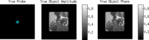
Figure 1: The true probe and object used in the generation of simulated dataset.

Let $x$ (respectively $y$) denote the true probe (true object). For the noiseless simulated data, we compute the measured data vectors using

$$b_{j}=|\mathcal{F}(S_{j}(x)\odot y)|\text{ for }j=1,2,\dots,m.$$

For the simulated data with noise, we use Poisson noise with mean/variance $\lambda=2$.

In typical ptychography experiments one more or less knows a priori what the probe looks like, though its precise structure, due to instrumentation aberrations, is unknown. The object, on the other hand, is assumed to be completely unknown except for certain qualitative properties, for example, that it is not absorbing. For the simulated data, the initial probe estimate consists of a circle of radius slightly larger than the true probe having constant amplitude and phase. Objects are initialized with a random initial guess. We demonstrate the stability of the algorithms in the results shown in Table 3 by purposely constraining the pupil to be smaller than the true pupil. This is not an unreasonable scenario since in practice the true pupil is not known.

Consistent with existing literature, we run several iterations of each algorithm without updating the probe to obtain a better initial object guess. The results of this “warm-up” procedure are then used as initial point $(x^{0},y^{0},\mathbf{z}^{0})$ for the main algorithm of which 300 iterations were performed. Experimentally, the “warm-up” procedure could also be accomplished with an “empty” beam data set consisting of beam images taken without specimen.

Where convenient, we use $u^{k}$ to denote $(x^{k},y^{k},\mathbf{z}^{k})$. Random trials of each problem instance were performed with random object initializations. Tables 1, 2 and 3 report the average, and in brackets, the worst result for the following statistics.

1. The final value of the least-squares objective given by (2.5).

2. The square of the norm of the change between the final two iterations, i.e., $\|u^{300}-u^{299}\|^{2}$.

3. The Root-mean-squared error of the final object and probe as described in [12]. The error is computed up to translation, a global phase shift and a global scaling factor.

4. The $R$-factor at iteration $300$, where

   $$R\text{-factor}^{k}=\frac{\sum_{j=1}^{m}\|b_{j}-S_{j}(x^{k})\odot y^{k}\|}{\sum_{j=1}^{m}b_{j}}.$$ (5.1)

   As in (2.7c), $b_{j}$ denotes the experimental observations.

5. The total time (seconds) for the “warm-up” and main algorithm.

Remark 5.1 (Error metrics).

Theorem 3.8(a) guarantees that the difference between the iterates of Algorithm 2.1 and Algorithm 3.4 converge in norm to zero. To compute the RMS-error a knowledge of the true object and probe are required, which in real applications are not known. The $R$-factor can still be evaluated in experimental settings (see Figure 3) and used as a measure of quality of the reconstruction, though the theoretical behavior of this metric is not covered by our analysis.

Table 1: Average (worst) results for noiseless simulated data.

Algorithm	$F(u^{300})$		$\|u^{300}-u^{299}\|^{2}$		RMS-Object		RMS-Probe		R-factor300		Time (s)
PHeBIE-I	$99.63$	$(126.64)$	$0.5931$	$(0.9383)$	$0.0410$	$(0.0461)$	$0.0155$	$(0.0222)$	$0.0131$	$(0.0154)$	$913.75$	$(925.85)$
PHeBIE-II	$70.76$	$(77.17)$	$0.2210$	$(0.3522)$	$0.0423$	$(0.0471)$	$0.0081$	$(0.0154)$	$0.0101$	$(0.0108)$	$636.74$	$(652.17)$
Rodenburg & Madien	$948.13$	$(1499.11)$	$5.5164$	$(8.4885)$	$0.0542$	$(0.0590)$	$0.0952$	$(0.1714)$	$0.0350$	$(0.0419)$	$1178.21$	$(1198.72)$
Thibault	$4347.08$	$(4554.28)$	$28.8622$	$(34.4422)$	$0.0515$	$(0.0642)$	$0.0240$	$(0.0378)$	$0.0244$	$(0.0264)$	$875.94$	$(887.76)$

Table 2: Average (worst) results for simulated data with Poisson noise.

Algorithm	$F(u^{300})$		$\|u^{300}-u^{299}\|^{2}$		RMS-Object		RMS-Probe		R-factor300		Time (s)
PHeBIE-I	$1.4415e+07$	$(6.9222e+07)$	$4.1504$	$(14.0823)$	$0.1928$	$(0.6840)$	$0.1896$	$(0.7084)$	$0.3499$	$(1.2698)$	$899.30$	$(933.54)$
PHeBIE-II	$1.4364e+07$	$(6.8972e+07)$	$521.9450$	$(2600.9689)$	$0.2807$	$(0.9940)$	$0.2537$	$(0.9746)$	$0.4001$	$(1.5135)$	$685.67$	$(714.21)$
Rodenburg & Madien	$6.7894e+04$	$(3.1414e+05)$	$14633.8000$	$(61868.3743)$	$0.2654$	$(0.9996)$	$0.3205$	$(0.9507)$	$0.3827$	$(1.2814)$	$1168.36$	$(1177.71)$
Thibault	$1.4520e+07$	$(6.9688e+07)$	$247.3130$	$(976.2039)$	$0.2476$	$(1.0000)$	$0.0700$	$(0.2498)$	$0.1748$	$(0.5686)$	$868.07$	$(892.19)$

Table 3: Average (worst) results for noiseless simulated data with over-restrictive pupil constraint.

Algorithm	$F(u^{300})$		$\|u^{300}-u^{299}\|^{2}$		RMS-Object		RMS-Probe		R-factor300		Time (s)
PHeBIE-I	$25653.20$	$(25656.12)$	$0.1474$	$(0.1682)$	$0.0443$	$(0.0501)$	$0.0492$	$(0.0494)$	$0.2936$	$(0.2937)$	$959.26$	$(1108.53)$
PHeBIE-II	$25653.80$	$(25660.13)$	$0.0622$	$(0.0852)$	$0.0314$	$(0.0356)$	$0.0496$	$(0.0499)$	$0.2936$	$(0.2937)$	$632.61$	$(645.10)$
Rodenburg & Madien	$3987.67$	$(4413.77)$	$6.2921$	$(16.3055)$	$0.0689$	$(0.0760)$	$0.0550$	$(0.0570)$	$0.2834$	$(0.2839)$	$1190.19$	$(1309.23)$
Thibault	$306602.00$	$(378554.38)$	$219.2110$	$(267.9303)$	$0.9432$	$(0.9437)$	$0.1898$	$(0.2435)$	$0.3634$	$(0.39160)$	$897.67$	$(962.45)$

For the noiseless simulated dataset, the quality of the reconstructed object and probe from each of the methods examined are comparable. This applies to the quantitative error metrics recorded in Table 1, as well as to a visual comparison of reconstructions (not shown). In the absence of noise, all the methods examined worked well. It is worth noting, that Algorithm 4.1 was significantly faster than all the other methods.

With the addition of Poisson noise, the quality of the reconstructed objects and probes deteriorates. The error metrics are mixed, and no clear “winner” emerges from the values reported in Table 2. The method of Thibault could be expected to be more unstable since it is based on the Douglas–Rachford algorithm, it has the advantage of pushing past local minima that might otherwise trap Algorithm 3.4.

The results for a improperly specified pupil constraint (too small) demonstrate the relative stability of the respective methods. The method of Thibault et al. was the most sensitive to the over-restrictive pupil constraint and performed the worst. This is expected since the modeling errors lead to inconsistency of the underlying feasibility problem: it is well known that Douglas–Rachford does not have fixed points for inconsistent feasibility problems [5]. Visually, the method of Thibault was not able to recover any semblance of the true solution. Algorithms 3.3 and 3.4 are clearly more robust. Visual comparisons also bear this out.

Tables 1, 2 and 3 suggest that is it not appropriate to compare the final objective value and stepsize of the various algorithms directly. Significant variability was exhibited in these metrics between the methods, despite all recording having similar RMS and $R$-factor errors in the ideal case of noiseless data.

5.2 Experimental Data

In this section we examine the four algorithms applied to an experimental data set (from [25]) in which the actual illumination function and specimen are unknown. The reconstructed illumination functions and specimens obtained from the four algorithms are shown in Figure 2. By visual inspection, the reconstructions are of comparable quality, with the exception of the results from method of Madien and Rodenburg, which is of noticeably poorer quality.

In Figure 3 compare two error metrics as a function of number of iterations for the four algorithms. The first graph, Figure 3(a) shows the norm of the difference of successive iterates, which, for PHeBIE, is the only quantity guaranteed to converge to zero by the theory we have developed above. The second graph, Figure 3(b) shows the $R$-factor which, as discussed in Remark 5.1 is computable in experimental settings. The best performance, with respect to both of these metrics, were observed for the fully decomposed parallel PHeBIE-II (Algorithm 4.1). We do not make any direct comparison with the reconstructions in [25], however, because there the authors implement routines beyond the scope of our theory. A more complete benchmarking study on experimental data is forthcoming.

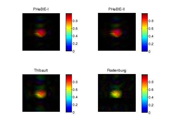
(a) Reconstructed probes.

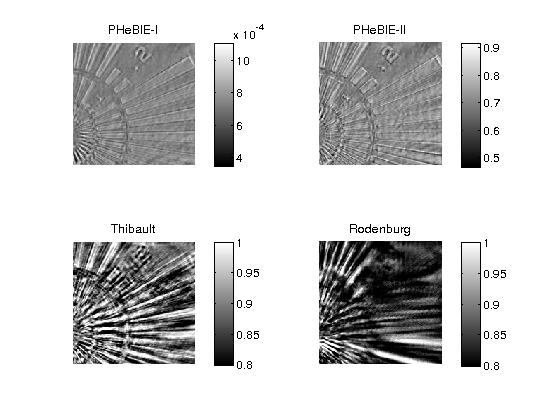
(b) Reconstructed specimen amplitudes.

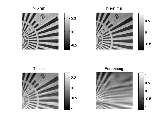
(c) Reconstructed specimen phases.

Figure 2: Results for the experimental dataset for the four different algorithms.

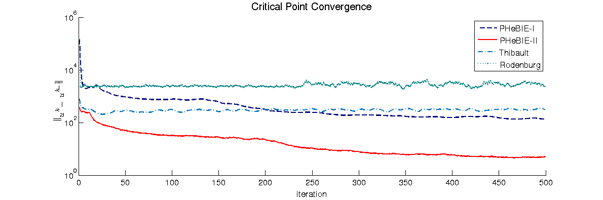
(a) The norm of the differences between successive iterates.

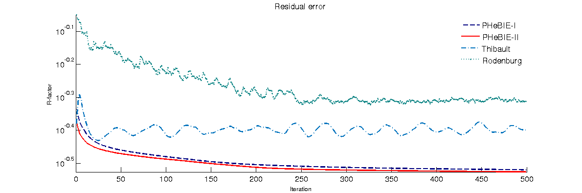
(b) The $R$-factor of the iterates defined by (5.1).

Figure 3: Performance profiles for the four algorithms applied to experimental data.

6 Appendix

6.1 Appendix A: Proof of Equations (4.3)-(4.6)

First, we compute the partial gradient of both functions.

$$\nabla_{x}F\left(x,y,{\bf z}\right) = 2\sum_{j=1}^{m}\left[S_{j}\left(\cdot\right)\odot y\right]^{\ast}\left(S_{j}\left(x\right)\odot y-z_{j}\right)=2\sum_{j=1}^{m}S_{j}^{\ast}\left(\overline{y}\odot\left(S_{j}\left(x\right)\odot y-z_{j}\right)\right)$$ (6.1)

$$= 2\sum_{j=1}^{m}\left[S_{j}^{\ast}\left(\overline{y}\odot y\right)\odot x-S_{j}^{\ast}\left(\overline{y}\odot z_{j}\right)\right]$$

and

$$\nabla_{y}F\left(x,y,{\bf z}\right) = 2\sum_{j=1}^{m}\left[S_{j}\left(x\right)\odot\left(\cdot\right)\right]^{\ast}\left(S_{j}\left(x\right)\odot y-z_{j}\right)=2\sum_{j=1}^{m}\overline{S_{j}\left(x\right)}\odot\left(S_{j}\left(x\right)\odot y-z_{j}\right)$$ (6.2)

$$= 2\sum_{j=1}^{m}\left[S_{j}\left(\overline{x}\odot x\right)\odot y-S_{j}\left(\overline{x}\right)\odot z_{j}\right],$$

where $S_{j}^{\ast}$, $j=1,2,\ldots,m$, denotes the adjoint transformation of $S_{j}$ and $\overline{z}$ denote the element-wise complex conjugate of $z$. We remind the reader that $S_{j}^{\ast}=S_{j}^{-1}$. We also used the following two facts:

$$\left[S_{j}\left(\cdot\right)\odot y\right]^{\ast}=S_{j}^{\ast}\left(\overline{y}\odot\left(\cdot\right)\right)\quad\text{and}\quad\left[S_{j}\left(x\right)\odot\left(\cdot\right)\right]^{\ast}=\overline{S_{j}\left(x\right)}\odot\left(\cdot\right).$$

Using (6.1) we obtain, for any $x,x^{\prime}\in\mathbb{C}^{n}$ that

$$\nabla_{x}F\left(x,y,{\bf z}\right)-\nabla_{x}F\left(x^{\prime},y,{\bf z}\right) =2\sum_{j=1}^{m}\left[S_{j}^{\ast}\left(\overline{y}\odot y\right)\odot x-S_{j}^{\ast}\left(\overline{y}\odot y\right)\odot x^{\prime}\right]$$

$$=2\sum_{j=1}^{m}S_{j}^{\ast}\left(\overline{y}\odot y\right)\odot\left(x-x^{\prime}\right)$$

$$=2\left(\sum_{j=1}^{m}S_{j}^{\ast}\left(\overline{y}\odot y\right)\right)\odot\left(x-x^{\prime}\right),$$ (6.3)

which means that

$$\left\|{\nabla_{x}F\left(x,y,{\bf z}\right)-\nabla_{x}F\left(x^{\prime},y,{\bf z}\right)}\right\|\leq 2\left\|{\sum_{j=1}^{m}S_{j}^{\ast}\left(\overline{y}\odot y\right)}\right\|_{\infty}\cdot\left\|{x-x^{\prime}}\right\|,$$

the last inequality follows from the following fact

$$\left\|{u\odot v}\right\|^{2}=\sum_{j=1}^{m}\left(u_{j}v_{j}\right)^{2}\leq\sum_{j=1}^{m}\left(\left|u_{j*}\right|\cdot\left|v_{j}\right|\right)^{2}=u_{j*}^{2}\sum_{j=1}^{m}v_{j}^{2}=\left\|{u}\right\|_{\infty}^{2}\left\|{v}\right\|^{2},$$

where $j*$ is the index of the largest entry in absolute value of $u$. This proves that

$$L_{x}\left(y,z\right)\leq 2\left\|{\sum_{j=1}^{m}S_{j}^{\ast}\left(\overline{y}\odot y\right)}\right\|_{\infty}.$$

On the other hand, choosing $x^{\prime}=0$ and $x=e_{i}$ (which is the $i$-th standard unit vector) and using (6.3) shows that

$$\nabla_{x}F\left(x,y,{\bf z}\right)-\nabla_{x}F\left(x^{\prime},y,{\bf z}\right)=2\left(\sum_{j=1}^{m}S_{j}^{\ast}\left(\overline{y}\odot y\right)\right)\odot e_{i}=2\left(\sum_{j=1}^{m}S_{j}^{\ast}\left(\overline{y}\odot y\right)\right)_{i},$$

where $(v)_{i}$ denotes the $i$-th component of the vector $v$. This means that we take $i=j*$, the largest entry in absolute value of $\sum_{j=1}^{m}S_{j}^{\ast}\left(\overline{y}\odot y\right)$, then we obtain that

$$\nabla_{x}F\left(x,y,{\bf z}\right)-\nabla_{x}F\left(x^{\prime},y,{\bf z}\right)=2\left\|{\sum_{j=1}^{m}S_{j}^{\ast}\left(\overline{y}\odot y\right)}\right\|_{\infty}.$$

This shows that

$$L_{x}\left(y,z\right)=2\left\|{\sum_{j=1}^{m}S_{j}^{\ast}\left(\overline{y}\odot y\right)}\right\|_{\infty}.$$

Similar arguments shows that

$$L_{y}\left(x,z\right)=2\left\|{\sum_{j=1}^{m}S_{j}\left(\overline{x}\odot x\right)}\right\|_{\infty}.$$

As a direct consequence of (6.3) we achieve

$$L_{x_{i}}\left(y,z\right)=2\left[\sum_{j=1}^{m}S_{j}^{\ast}\left(\overline{y}\odot y\right)\right]_{i}$$

and by similar argument

$$L_{y_{i}}\left(x,z\right)=2\left[{\sum_{j=1}^{m}S_{j}\left(\overline{x}\odot x\right)}\right]_{i}$$

which are (4.5) and (4.6) respectively. $\Box$

Remark 6.1 (Block partial Lipschitz constants).

For more general variable blocks of the form considered in Section 3.3, the corresponding formula for $L_{x_{i}}(y,z)$ (resp. $L_{y_{i}}(x,z)$) are given by taking twice largest entry in the block $X_{i}$ (resp. $Y_{i}$) from the summation. That is,

$$L_{x_{i}}\left(y,z\right)=2\left\|\left.\left(\sum_{j=1}^{m}S_{j}^{\ast}\left(\overline{y}\odot y\right)\right)\right|_{X_{i}}\right\|_{\infty},\quad L_{y_{i}}\left(x,z\right)=2\left\|\left.\left(\sum_{j=1}^{m}S_{j}\left(\overline{x}\odot x\right)\right)\right|_{Y_{i}}\right\|_{\infty},$$

where $|_{X_{i}}$ (res. $|_{Y_{i}}$) denotes the restriction to the block $X_{i}$ (resp. $Y_{i}$).

From these formulae one immediately recovers (4.5) and (4.6) as special cases.

References

- [1] J. M. Rodenburg. Ptychography and related diffractive imaging methods. Adv. Imaging Electron Phys., 150:87–184, 2008.
- [2] H. Attouch and J. Bolte. On the convergence of the proximal algorithm for nonsmooth functions involving analytic features. Math. Program., 116:5–16, 2009.
- [3] H. Attouch, J. Bolte, P. Redont, and A. Soubeyran. Proximal alternating minimization and projection methods for nonconvex problems: an approach based on the Kurdyka-Łojasiewicz inequality. Math. Oper. Res., 35:438–457, 2010.
- [4] H. Attouch, J. Bolte, and B. F. Svaiter. Convergence of descent methods for semi-algebraic and tame problems: proximal algorithms, forward-backward splitting, and regularized Gauss-Seidel methods. Math. Program., 137:91–129, 2013.
- [5] H. H. Bauschke, P. L. Combettes, and D. R. Luke. Finding best approximation pairs relative to two closed convex sets in Hilbert spaces. J. Approx. Theory, 127:178–192, 2004.
- [6] A. Beck and M. Teboulle. A fast iterative shrinkage-thresholding algorithm for linear inverse problems. SIAM J. Imaging Sci., 2:183–202, 2009.
- [7] J. Bolte, A. Daniilidis, and A. Lewis. The Łojasiewicz inequality for nonsmooth subanalytic functions with applications to subgradient dynamical systems. SIAM J. Optim., 17:1205–1223, 2006.
- [8] J. Bolte, A. Daniilidis, A. Lewis, and M. Shiota. Clarke subgradients of stratifiable functions. SIAM J. on Optimization, 18:556–572, 2007.
- [9] J. Bolte, S. Sabach, and M. Teboulle. Proximal alternating linearized minimization for nonconvex and nonsmooth problems. Math. Program., Ser. A,146:459–494 (2014).
- [10] P. L. Combettes and V. R. Wajs. Signal recovery by proximal forward-backward splitting. Multiscale Model. Simul., 4:1168–1200, 2005.
- [11] J. Douglas and H. H. Rachford. On the numerical solution of heat conduction problems in two or three space variables. Trans. Amer. Math. Soc., 82:421–439, 1956.
- [12] M. Guizar-Sicairos, S.T. Thurman, and J.R. Fienup. Efficient subpixel image registration algorithms. Optics letters, 33(2):156–158, 2008.
- [13] R. Hegerl and W. Hoppe. Dynamische theorie der kristallstrukturanalyse durch elektronenbeugung im inhomogenen primärstrahlwellenfeld. Ber. Bunsenges. Phys. Chem, 74(11):1148–1154, 1970.
- [14] P. L. Lions and B. Mercier. Splitting Algorithms for the Sum of Two Nonlinear Operators. SIAM Journal on Numerical Analysis, 16(6):964–979, 1979.
- [15] D. R. Luke. Finding best approximation pairs relative to a convex and a prox-regular set in a Hilbert space. SIAM J. Optim., 19:714–739, 2008.
- [16] D. R. Luke, J. V. Burke, and R. G. Lyon. Optical wavefront reconstruction: theory and numerical methods. SIAM Rev., 44:169–224, 2002.
- [17] D.R. Luke. Relaxed averaged alternating reflections for diffraction imaging. Inverse Problems, 21(1):37, 2005.
- [18] A. M. Maiden and J. M. Rodenburg. An improved ptychographical phase retrieval algorithm for diffractive imaging. Ultramicroscopy, 109:1256–1262, 2009.
- [19] J. Qian, C. Yang, A. Schirotzek, F. Maia, and S. Marchesini. Efficient algorithms for ptychographic phase retrieval. Contemporary Mathematics, 2014.
- [20] R. T. Rockafellar and R. J. Wets. Variational Analysis. Grundlehren der mathematischen Wissenschaften. Springer-Verlag, Berlin, 1998.
- [21] J. M. Rodenburg and R. H. T. Bates. The theory of super-resolution electron microscopy via wigner-distribution deconvolution. Philos. Trans. R. Soc. London Ser. A, 339:521–553, 1992.
- [22] J. M. Rodenburg, A. C. Hurst, A. G. Cullis, B. R. Dobson, F. Pfeiffer, O. Bunk, C. David, K. Jefimovs, and I. Johnson. Hard-x-ray lensless imaging of extended objects. Phys. Rev. Lett., 98:034801, 2007.
- [23] Y. Shechtman, Y. C. Eldar, O. Cohen, H. N. Chapman, J. Miao and M. Segev. Phase retrieval with application to optical imaging. IEEE Magazine, 2014.
- [24] P. Thibault, M. Dierolf, O. Bunk, A. Menzel, and F. Pfeiffer. Probe retrieval in ptychographic coherent diffractive imaging. Ultramicroscopy, 109:338–343, 2009.
- [25] R. N. Wilke, M. Priebe, M. Bartels, K. Giewekemeyer, A. Diaz, P. Karvinen, and T. Salditt. Hard X-ray imaging of bacterial cells: nano-diffraction and ptychographic reconstruction. Optics Express, 20(17):19232–19254, 2012.