Rough surface backscatter and statistics via extended parabolic integral equation

Abstract

This paper extends the parabolic integral equation method, which is very effective for forward scattering from rough surfaces, to include backscatter. This is done by applying left-right splitting to a modified two-way governing integral operator, to express the solution as a series of Volterra operators; this series describes successively higher-order surface interactions between forward and backward going components, and allows highly efficient numerical evaluation. This and equivalent methods such as ordered multiple interactions have been developed for the full Helmholtz integral equations, but not previously applied to the parabolic Green’s function. In addition, the form of this Green’s function allows the mean field and autocorrelation to be found analytically to second order in surface height. These may be regarded as backscatter corrections to the standard parabolic integral equation method.

Department of Applied Mathematics and Theoretical Physics, The University of Cambridge CB3 0WA, UK

1 Introduction

Wave scattering from irregular surfaces continues to present formidable theoretical and computational challenges [1, 2, 3, 4, 5, 6, 7], especially with regard to analytical treatment of statistics, and numerical solution for wave incidence at low grazing angles [8, 9, 10, 11, 12, 13], where the insonified/illuminated region may become very large. Computationally, the cost of the necessary matrix inversion scales badly with wavelength and domain size and can rapidly become prohibitive; this is compounded by the large number of Green’s function evaluations, whose overall cost is therefore sensitive to the form which this function takes.

Under the assumption of purely forward-scattering, a successful approach has been the parabolic integral equation method (PIE)[14, 15, 16]. This makes use of a ‘one-way’ parabolic equation (PE) Green’s function, leading to the replacement of the Helmholtz integral equations by their small-angle analogue. For 2D problems this Green’s function takes a particularly tractable form; this, together with the Volterra (one-sided) form of the governing integral operator, affords the key advantage of high numerical efficiency, and in the perturbation regime allows derivation of analytical results [17, 18, 19, 20]. Nevertheless, the method yields no information about the field scattered back towards the source.

On the other hand, where backscatter is required, operator series solution methods such as left-right splitting and method of ordered multiple interactions [21, 22, 23, 24, 25, 26, 27] have proved highly versatile, in both 2 and 3 dimensions. These use the full free-space Green’s function and proceed by expanding the surface fields about the dominant ‘forward-going’ component, and thereby circumvent the difficulties of tackling the full Helmholtz equations.

In this paper we combine these approaches, extending the standard PIE description to a ‘two-way’ method, thus allowing for both left- and right-travelling waves. This is obtained in the obvious way by replacing the parabolic equation Green’s function by a form symmetrical in range. The integral operator can be split into left- and right-going parts; under the assumption that forward scattering dominates, the solution can then be written as a series and truncated. Every term of this series is a product of Volterra operators and is therefore treated as efficiently as the standard PIE method, which corresponds approximately to truncation at the first term.

In the second part of the paper we impose the additional restriction to the perturbation regime of small surface height $\sigma$, within which analytical expressions for the mean field and autocorrelation function are obtained. This extends the corresponding results[17, 18] derived under the PIE method. The approach there was first to obtain the scattered field to second order in $\sigma$ at the mean surface plane, and find the far-field under the assumption that propagation outwards from the surface is governed by the full Helmholtz equation. In the standard PE case, this modification allows a small amount of backscatter, but precludes any backscatter enhancement which can be thought of as due to coherent addition of reversible paths[29, 30, 31], because interactions at the surface are assumed to be take place in the forward direction only. The formulation presented here allows one to remove this restriction, and separate the forward and backward going interactions to various orders, although this aspect is not explored in detail here. In particular this method produces a correction term, whose statistics can be obtained in the perturbation regime.

The paper is organised as follows: The standard parabolic integral equation method and preliminary results are given in section 2. In section 3 the full two-way parabolic integral equation method is set out, and the iterative solution explained. Analytical results for the statistics under the extended method are derived in section 4.

2 Parabolic integral equation method and preliminaries

We consider the problem of a scalar time-harmonic wave field $p$ scattered from a one-dimensional rough surface $h(x)$ with a pressure release boundary condition. (Equivalently, $p$ is an electromagnetic $s$ or $TE$ polarised wave and $h$ is a perfectly conducting corrugated surface whose generator is in the plane of incidence.) The wavefield has wavenumber $k$ and is governed by the wave equation $(\nabla^{2}+k^{2})p=0$. The coordinate axes are $x$ and $z$ where $x$ is the horizontal and $z$ is the vertical, directed out of the medium (see Fig. 1). Angles of incidence and scatter are assumed to be small with respect to the positive $x$-direction. It will be assumed that the surface is statistically stationary to second order, i.e. its mean and autocorrelation function are translationally invariant. We may choose coordinates so that $h(x)$ has mean zero. The autocorrelation function $<h(x)h(x+\xi)>$ is denoted by $\rho(\xi)$, and we assume that $\rho(\xi)\rightarrow 0$ at large separations $\xi$. (The angled brackets here denote the ensemble average.) Then $\sigma^{2}\equiv\rho(0)$ is the variance of surface height, so that the surface roughness is of order $O(\sigma)$.

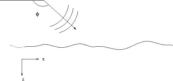
Figure 1: Schematic view of scattering geometry

Since the field components propagate predominantly around the $x$-direction, we can define a slowly-varying part $\psi$ by

$$\psi(x,z)~{}=~{}p(x,z)~{}\exp(-ikx).$$ (1)

Slowly varying incident and scattered components $\psi_{i}$ and $\psi_{s}$ are defined similarly, so that $\psi=\psi_{i}+\psi_{s}$. It may be assumed that $\psi_{i}(x,h(x))=0$ for $x\leq 0$, so that the area of surface insonification is restricted, as it would be for example in the case of a directed Gaussian beam. The governing equations for the standard parabolic equation method [14, 15] are then

$$\psi_{i}({\bf r}_{s})=-\int_{0}^{x}~{}G_{p}({\bf r}_{s};{\bf r^{\prime}})\frac{\partial\psi({\bf r^{\prime}})}{{\partial z}}~{}dx^{\prime}$$ (2)

where both ${\bf r}_{s}=(x,h(x))$, ${\bf r^{\prime}}=(x^{\prime},h(x^{\prime}))$ lie on the surface; and

$$\psi_{s}({\bf r})=\int_{0}^{x}~{}G_{p}({\bf r};{\bf r^{\prime}})\frac{\partial\psi({\bf r^{\prime}})}{{\partial z}}~{}dx^{\prime}$$ (3)

where ${\bf r^{\prime}}$ is again on the surface and ${\bf r}$ is an arbitrary point in the medium. Here $G_{p}$ is the parabolic form of the Green’s function in two dimensions given by

$$G_{p}(x,z;x^{\prime},z^{\prime})\left\{\begin{array}[]{lr}=&\alpha~{}{\sqrt{1\over x-x^{\prime}}}~{}\exp\Bigl{[}{ik(z-z^{\prime})^{2}\over 2(x-x^{\prime})}\Bigr{]}\hfill~{}~{}~{}~{}~{}~{}{\rm for~{}}x^{\prime}~{}<~{}x\\ =&0\hfill~{}~{}~{}~{}~{}~{}~{}~{}~{}~{}~{}~{}~{}~{}{\rm otherwise}\end{array}\right.$$

where $\alpha={1\over 2}~{}{\sqrt{i/2\pi k}}$. This asymmetrical form gives rise to the finite upper limit of integration in (2) and (3). It is derived under the assumption of forward-scattering, and that the field obeys the parabolic wave equation,

$$\psi_{x}~{}+~{}2ik\psi_{zz}~{}=~{}0$$ (4)

which holds provided the angles of incidence and scattering are fairly small with respect to the $x$-direction. ($G_{p}$ can also be obtained directly from the full free space Green’s function under the small-angle approximation.) Equation (2) must be inverted to give the induced source $\partial\psi/\partial z$ at the surface, which is then substituted in (3) to determine the field elsewhere.

Now, equations (2) and (3) do not apply to plane wave scattering at small or negative $x$ because of the truncated lower limit of integration, equivalent to the restricted surface insonification. Nevertheless, we can formally apply the integral equation to a plane wave, to obtain a solution which will be physically meaningful and asymptotically accurate at large values of $x$. This procedure has been used[17, 18] to derive the field statistics; where necessary we will assume that $x$ is sufficiently large for this to hold.

Consider an incident plane wave $p=\exp(ik[x\sin\theta+z\cos\theta])$, where $\theta$ is the angle with respect to the vertical. The grazing angle is then denoted $\mu=\pi/2-\theta$ (see Fig. 1). This plane wave has slowly-varying component $\psi^{\theta}=\exp(ik[Sx+z\cos\theta])$, where

$$S~{}=~{}\sin\theta-1,$$ (5)

which we refer to as the reduced plane wave.

3 Two-way parabolic integral equation method

In this section the two-way version of the PIE method will be described, and the iterative solution will be given. This provides an efficient means of calculating the back-scattered component at small angles of scatter.

3.1 The modified governing equations

The governing equations (2), (3) must first be modified to take into account scattering from the right. To do this, we simply replace $G_{p}$ by its symmetrical analogue $G$. This form arises if we apply the small angle approximation described in section 2 to the full free space Green’s function without requiring $G(x,z;x^{\prime},z^{\prime})$ to vanish when $x^{\prime}\geq x$. We thus obtain

$$G(x,z;x^{\prime},z^{\prime})~{}\left\{\begin{array}[]{lr}{}&=~{}\alpha~{}{\sqrt{1\over x-x^{\prime}}}~{}\exp\Bigl{[}{ik(z-z^{\prime})^{2}\over 2(x-x^{\prime})}\Bigr{]}\hfill~{},~{}~{}~{}~{}~{}~{}~{}~{}~{}~{}~{}~{}~{}~{}~{}~{}~{}~{}~{}~{}~{}~{}x^{\prime}~{}<~{}x\cr{}&=~{}\alpha~{}{\sqrt{1\over x^{\prime}-x}}~{}\exp\Bigl{[}{ik(z-z^{\prime})^{2}\over 2(x^{\prime}-x)}\Bigr{]}~{}\exp\left[2ik(x^{\prime}-x)\right]~{}~{}~{}~{}~{}~{}~{}x^{\prime}~{}\geq~{}x\end{array}\right.$$ (6)

The factor $\exp[-2ik(x^{\prime}-x)]$ arises for $x^{\prime}\geq x$ because we are solving for the reduced wave $\psi$.

Applying this Green’s function to the reduced wave $\psi$ we obtain

$$\psi_{s}(x,z)=\int_{0}^{\infty}G({\bf r},{\bf r}^{\prime}){\partial\psi({\bf r}^{\prime})\over\partial z}dx^{\prime}$$ (7)

where ${\bf r}=(x,z)$, ${\bf r}^{\prime}=(x^{\prime},h(x^{\prime}))$. This is the analogue of equation (2), effectively containing a back-scatter correction. Taking the limit of (7) as $z\rightarrow h(x)$ yields an integral equation relating the incident field to the scattered field at the surface:

$$\psi_{i}(x,h(x))=-\int_{0}^{\infty}G({\bf r}_{s},{\bf r}^{\prime}){\partial\psi({\bf r}^{\prime})\over\partial z}dx^{\prime}$$ (8)

where now ${\bf r}_{s}=(x,h(x))$, ${\bf r}^{\prime}=(x^{\prime},h(x^{\prime}))$ both lie on the surface. (Note that the addition of a correction to the parabolic equation is closely related to a method proposed by Thorsos[14].) Equations (7), (8) can be written in operator notation:

$$\psi_{s}(x,z)=-(L+R){\partial\psi\over\partial z}$$ (9)

$$\psi_{i}(x,h(x))=(L+R){\partial\psi\over\partial z}$$ (10)

where $L$, $R$ are defined by

$$Lf(x,z)=\int_{0}^{x}G({\bf r},{\bf r}^{\prime})f(x^{\prime})dx^{\prime},~{}~{}~{}~{}~{}Rf(x,z)=\int_{x}^{\infty}G({\bf r},{\bf r}^{\prime})f(x^{\prime})dx^{\prime}$$

and ${\bf r}=(x,z)$, ${\bf r}^{\prime}=(x^{\prime},h(x^{\prime}))$. These integral operators and their inverses are Volterra, or ‘one-sided’ in an obvious sense.

3.2 Solution of the modified equations

The main computational task in any such boundary integral method is the inversion of the integral equation (10). One of the principal advantages of the standard forward-going PIE method (equations (2)-(3)) is that its one-way form allows Gaussian elimination to be used, so that inversion is highly efficient. In the above two-way formulation this advantage is initially lost, since direct inversion of $L+R$ in eq. (10) offers no benefit compared with solving the full Helmholtz equations. However, the computational advantage can be regained by forming an iterative series solution, in which each term is a product of Volterra integral operators.

Integral equation (10) has formal solution

$${\partial\psi\over\partial z}=(L+R)^{-1}\psi_{i}$$ (11)

which can be expanded in a series

$${\partial\psi\over\partial z}=\left[L^{-1}-L^{-1}RL^{-1}+\left(L^{-1}R\right)^{2}L^{-1}-...\right]\psi_{i}$$ (12)

Under the assumption that $R$ is small in the following sense the series (12) is convergent, as is already required implicitly for the standard PIE solution; the series can then be truncated after finitely many terms. By ‘small’ we mean that $R\phi/||\phi||$ is small for all terms $\phi$ in the series. It can be shown that this assumption is indeed justified at low grazing angles for surfaces whose slopes are not too large, since the kernel of $R$ oscillates rapidly especially at small wavelengths. It is nevertheless difficult to give this a precise range of validity, and we will not attempt to do so here.

Solution for the field can therefore be obtained by truncating the series (12) and substituting into the integral (7). The first term $L^{-1}\psi_{i}$ in series (12) corresponds to the solution for $\partial\psi/\partial z$ under the standard PIE method (e.g. [15]). Denote this first approximation by ${\tilde{\psi}}$, i.e.

$${\partial\psi\over\partial z}\cong{\tilde{\psi}}=L^{-1}\psi_{i}.$$ (13)

Note however that the integral (7) allows for outgoing components scattered to the left, unlike its PIE analogue (3), so even this lowest order truncation gives backscatter. This can be considered the direct backscatter component.

Truncation of (12) at the second term gives:

$${\partial\psi\over\partial z}\cong{\tilde{\psi}}+C$$ (14)

where $C$ is a correction term,

$$C=L^{-1}RL^{-1}\psi_{i}.$$ (15)

The above expression will be used in section 4 to obtain some statistical measure of the backscattered component in the perturbation regime of small surface height. We remark that this is the lowest-order truncation consistent with reversible ray paths.

3.3 Numerical evaluation

The general term of (12) is a product of the operators $L^{-1}$ and $R$. Evaluation of the integral $R$ is straightforward. For computational purposes we assume that the incident wave insonifies only a finite region of the rough surface; the source may for example be a Gaussian beam. A finite upper limit of integration $x_{max}$, say, may then be assumed.

Numerical inversion of $L$ is also highly efficient since discretization of $L$ gives rise to a lower-triangular matrix. This has been described elsewhere (e.g. [15]) and will only be summarized here.

Consider the equation $L\partial\psi/\partial z=\psi_{i}$ obtained by truncating (12) at the first term. This equation is discretized with respect to range $x$ using, say, $N$ equally spaced points $x_{j}$. This then yields a matrix equation $A\partial\psi/\partial z=\psi_{i}$ in which the matrix $A$ is lower-triangular. Numerical inversion of this expression is carried out by Gaussian elimination, requiring $O(N^{2})$ operations, which compares with $O(N^{3})$ operations required to treat the full Helmholtz integral equation.

The solution is thereby obtained for the first term, ${\tilde{\psi}}$. Typically only one further term, $L^{-1}R{\tilde{\psi}}$, will be required. The simplest way to obtain this is to discretize the integral $R$, evaluate $R{\tilde{\psi}}$ numerically, and then to solve

$$L^{-1}R{\tilde{\psi}}={\partial\psi\over\partial z}-{\tilde{\psi}}$$

by Gaussian elimination as before. The evaluation of the integral $R$ also requires $O(N^{2})$ operations. Subsequent terms in the series may be obtained similarly.

The computation can be simplified further in the perturbation regime of small scaled surface height $k\sigma$, if the operators $L$ and $R$ are replaced by the flat surface forms in the calculation of the correction term $C$. This is described in the section 4.

4 Perturbation solution and statistics of backscatter

4.1 Perturbation solution

The mean field and higher moments based on the standard parabolic equation approximation were obtained elsewhere[17, 18] to second order in surface height in the case of pure forward scattering. In this section the statistics of the backscatter correction (eq. (14)) due to the two-way PIE method will be derived.

Suppose that a reduced plane wave $\psi_{i}^{\theta}=\exp(ik[xS+z\cos\theta])$ is incident on the rough surface at an angle $\theta$ measured from the normal. We first summarize the perturbational calculation used to obtain the scattered field statistics previously. Suppose that a plane $z=z_{1}$, say, can be chosen ‘close’ to every point on the surface. The scattered field is obtained to second order in surface height along this plane, for a given incident plane wave, and the statistics are found from this. Statistical results obtained in this way do not depend on the choice of $z_{1}$ so for convenience we may set $z_{1}=0$. An expression is thus found for the scattered field

$$\psi_{s}(x,0)~{}=~{}-\psi_{i}^{\theta}(x,h)-h\left[{\partial\psi\over\partial z}-{\partial\psi_{i}\over\partial z}\right]-{1\over 2}h^{2}{\partial^{2}\psi_{i}(x,0)\over\partial z^{2}}~{}+~{}O(\sigma^{3}).$$ (16)

The only term here which is not known a priori is $\partial\psi/\partial z$. The standard PIE solution ${\tilde{\psi}}$ for $\partial\psi/\partial z$ is given[17, 18] to second order in $\sigma$ by:

$${\partial\psi\over\partial z}\cong{\tilde{\psi}}=-{1\over\pi}~{}{d~{}\over dx}\int_{0}^{x}~{}{\psi_{i}^{\theta}(x^{\prime},h(x^{\prime}))\over\alpha\sqrt{x-x^{\prime}}}~{}dx^{\prime}.$$ (17)

This arises from (13) by substitution of the flat surface form of $L$ (see (20) below). Denote by ${\tilde{\psi}_{s}}$ the approximation to $\psi_{s}$ obtained by substituting (17) in (16), so that

$$\tilde{\psi}_{s}(x,0)~{}\equiv~{}~{}-~{}\psi_{i}^{\theta}(x,h) +h~{}\biggl{[}{1\over\pi}~{}{d~{}\over dx}\int_{0}^{x}~{}{\psi_{i}^{\theta}(x^{\prime},h(x^{\prime}))\over\alpha\sqrt{x-x^{\prime}}}~{}dx^{\prime}~{}+~{}{\partial\psi_{i}^{\theta}(x,h)\over\partial z}\biggr{]}$$ (18)

$$-~{}{h^{2}\over 2}{\partial^{2}\psi_{i}^{\theta}(x,0)\over\partial z^{2}}.$$

We wish to calculate the backscatter correction to this expression due to the replacement of $\partial\psi/\partial z$ in (16) by the corrected two-way PE solution $({\tilde{\psi}}+C)$ (equations (14), (15)). We therefore repeat the above derivation replacing (13) by (14), to obtain

$$\psi_{s}(x,0)={\tilde{\psi}_{s}}(x,0)+h(x)C(x).$$ (19)

Since the correction term $C$ appears here with a factor $h$, it is necessary to evaluate it only to order $O(\sigma)$.

Expanding $L$ and $R$ (eqs. (9)-(10)) in surface height $h(x)$, it is seen that $L=L_{0}+O(\sigma^{2})$, $R=R_{0}+O(\sigma^{2})$, where $L_{0}$, $R_{0}$ denote the deterministic (i.e. flat surface) forms of the operators $L$ and $R$ respectively:

$$L_{0}=\alpha\int_{0}^{x}{1\over\sqrt{x-x^{\prime}}}~{}dx^{\prime},~{}~{}~{}~{}~{}R_{0}=\alpha\int_{x}^{\infty}{1\over\sqrt{x^{\prime}-x}}~{}dx^{\prime}$$ (20)

In evaluating $C$ (eq. (15)) to order $O(\sigma)$ we may thus ignore fluctuating parts of the operators, and replace $L$, $R$ by $L_{0}$, $R_{0}$ respectively. We can therefore write

$$C=L_{0}^{-1}R_{0}{\tilde{\psi}}+O(\sigma^{2}).$$ (21)

An expression of the form $f=L_{0}^{-1}g$ is Abel’s integral equation, which has the well-known solution[28]

$$g(x)={1\over\alpha\pi}{d\over dx}\int_{0}^{x}{1\over\sqrt{x-y}}f(y)dy.$$

Now to first order in $h$, ${\tilde{\psi}}$ in (21) is given[17] by

$${\tilde{\psi}}(r)\cong-\pi\left[D_{\theta}(r)+{dI(r)\over dr}\right].$$ (22)

where, for large $r$, $D$ takes the form (see eq. (15) of [17])

$$D_{\theta}(r)\sim-2ik\pi\sqrt{2-2\sin\theta}e^{ikSr}$$ (23)

and $I$ is an integral

$$I(r)~{}=~{}~{}\int_{0}^{r}~{}ikh(r^{\prime})\cos\theta{e^{ikSr^{\prime}}\over\alpha\sqrt{r-r^{\prime}}}~{}dr^{\prime}.$$ (24)

Therefore $D$ and $dI/dr$ are $O(1)$ and $O(h)$ respectively, so that in eq. (21) $C$ becomes

$$C(x)={1\over\alpha^{2}\pi}{d\over dx}\left[\int_{0}^{x}{1\over\sqrt{x-y}}\int_{y}^{\infty}{\exp(ikr)\over\sqrt{y-r}}{\tilde{\psi}}(r)~{}dr~{}dy\right].$$ (25)

To second order in surface height the scattered field $\psi_{s}(x,0)$ at the mean surface is therefore described by eq. (19), with $C$ given by (25).

4.2 Mean field

The effect of the correction term $C$ on the scattered field statistics can now be examined. We first find the mean field $<\psi_{s}(x,z)>$. It is sufficient to obtain this quantity on the mean surface plane $z=0$, using equation (19), i.e.

$$<\psi_{s}(x,0)>~{}=~{}<\tilde{\psi}_{s}(x)>+<h(x)C(x)>.$$

The solution for $<\tilde{\psi}_{s}>$ has been obtained previously[17], and we can restrict attention to finding the correction $<hC>$ to this. Denote the correlation $<h(X)C(x)>$ by ${\cal E}$ for any $X$, $x$, i.e.

$${\cal E}(X,x)=<h(X)C(x)>.$$

Consider first the function $<h{\tilde{\psi}}>$. Since $<hD_{\theta}>$ vanishes, eq. (22) gives

$$<h{\tilde{\psi}}>=-\pi<h{\partial I\over\partial x}>.$$ (26)

Now from eq. (25)

$${\cal E}(X,x)=\left<{h(X)\over\alpha^{2}\pi}~{}{d\over dx}\int_{0}^{x}{1\over\sqrt{x-y}}\int_{y}^{\infty}{\exp(ikr)\over\sqrt{y-r}}{\tilde{\psi}}(r)~{}dr~{}dy\right>.$$

The term $h(X)$ can be taken under the integral signs as part of the operand of $d/dx$. The order of integration and averaging can then be reversed so that, by (26),

$${\cal E}(X,x)=-{1\over\alpha^{2}}\left[{d\over dx}\int_{0}^{x}{1\over\sqrt{x-y}}\int_{y}^{\infty}{e^{ikr}\over\sqrt{y-r}}\left<h(X){\partial I(r)\over\partial r}\right>~{}dr~{}dy\right].$$ (27)

Consider the term $<h(X)dI/dr>$ in the inner integrand. By (24),

$$\left<h(X){\partial I(r)\over\partial r}\right>= \left<h(X){d\over dr}~{}\int_{0}^{r}~{}ikh(r^{\prime})\cos\theta{e^{ikSr^{\prime}}\over\alpha\sqrt{r-r^{\prime}}}~{}dr^{\prime}\right>$$ (28)

$$~{}= ik\cos\theta{d\over dr}\left[~{}\int_{0}^{r}~{}{e^{ikSr^{\prime}}\over\alpha\sqrt{r-r^{\prime}}}\rho(X-r^{\prime})~{}dr^{\prime}\right]$$

This may be substituted into (27) to give an analytical expression for the correlation $<h(X)C(x)>$. We can simplify this expression by evaluating the derivatives explicitly. The term $\rho(X-r^{\prime})$ is independent of $r$, so writing

$${e^{ikSr^{\prime}}\over\alpha\sqrt{r-r^{\prime}}}=f(r,r^{\prime})$$ (29)

the expression (28) becomes

$$\left<h(X){\partial I(r)\over\partial r}\right>=ik\cos\theta{d\over dr}\left[~{}\int_{0}^{r}~{}f(r,r^{\prime})\rho(X-r^{\prime})~{}dr^{\prime}\right]$$

$$= ik\cos\theta~{}\lim_{\epsilon\rightarrow 0}{1\over\epsilon}\left[\int_{0}^{r+\epsilon}f(r+\epsilon,r^{\prime})\rho(X-r^{\prime})dr^{\prime}-\int_{0}^{r}f(r,r^{\prime})\rho(X-r^{\prime})dr^{\prime}\right]$$ (30)

$$= ik\cos\theta~{}\lim_{\epsilon\rightarrow 0}{1\over\epsilon}\left[K_{1}+K_{2}-K_{3}\right]$$

where

$$K_{1} =\int_{0}^{\epsilon}f(r+\epsilon,r^{\prime})\rho(X-r^{\prime})dr^{\prime}$$

$$K_{2} =\int_{\epsilon}^{r+\epsilon}f(r+\epsilon,r^{\prime})\rho(X-r^{\prime})dr^{\prime}$$ (31)

$$K_{3} =\int_{0}^{r}f(r,r^{\prime})\rho(X-r^{\prime})dr^{\prime}$$

Consider these three integrals in detail. The first gives

$${1\over\epsilon}K_{1}={1\over\epsilon}\int_{0}^{\epsilon}f(r+\epsilon,r^{\prime})\rho(X-r^{\prime})dr^{\prime}\cong{1\over\epsilon}\rho(X)\int_{0}^{\epsilon}{1\over\sqrt{r+\epsilon-r^{\prime}}}dr^{\prime}$$

$$= {2\over\alpha\epsilon}\rho(X)\left[\sqrt{r+\epsilon}-\sqrt{r}\right]$$ (32)

$$\cong {\rho(X)\over\alpha\sqrt{r}}$$

using a Taylor expansion in $\epsilon$. Changing variables, $K_{2}$ in can be written

$$\int_{\epsilon}^{r+\epsilon}f(r+\epsilon,r^{\prime})\rho(X-r^{\prime})dr^{\prime}=\int_{0}^{r}f(r+\epsilon,r^{\prime\prime}+\epsilon)\rho(X-r^{\prime\prime}-\epsilon)dr^{\prime\prime}.$$ (33)

Now

$$f(r+\epsilon,r^{\prime\prime}+\epsilon)={e^{ikS(r^{\prime\prime}+\epsilon)}\over\alpha\sqrt{r-r^{\prime\prime}}}=e^{ikS\epsilon}f(r,r^{\prime\prime}$$

so from (33)

$$\int_{\epsilon}^{r+\epsilon}f(r+\epsilon,r^{\prime})\rho(X-r^{\prime})dr^{\prime}=\int_{0}^{r}e^{ikS\epsilon}f(r,r^{\prime})\rho(X-r^{\prime}-\epsilon)dr^{\prime}.$$ (34)

Thus the difference $K_{2}-K_{3}$ in (30) becomes

$$\int_{0}^{r}f(r,r^{\prime})\left[e^{ikS\epsilon}\rho(X-r^{\prime}-\epsilon)-\rho(X-r^{\prime})\right]dr^{\prime}$$ (35)

$$\cong \int_{0}^{r}f(r,r^{\prime})\epsilon\left[ikS\rho(X-r^{\prime})-{d\rho(X-r^{\prime})\over dX}\right]dr^{\prime}$$

where $\rho$, which may be assumed to be differentiable, has been expanded to leading order in $\epsilon$. Substituting (32) and (35) in (28), we obtain

$$\left<h(X){\partial I(r)\over\partial r}\right>={ik\over\alpha}\cos\theta\left\{{\rho(X)\over\sqrt{r}}+\int_{0}^{r}{e^{ikSr^{\prime}}\over\sqrt{r-r^{\prime}}}\left[ikS\rho(X-r^{\prime})-{d\rho(X-r^{\prime})\over dX}\right]dr^{\prime}\right\}.$$ (36)

This removes the derivative with respect to $x$ in (27), and indeed for several important autocorrelation functions eq. (36) can be written in closed form. The term $\rho(X)/\sqrt{r}$ is an artifact of the finite lower bound of integration and can be dropped, as we can assume the range variable $X$ to be large. Equation (27) therefore becomes

$${\cal E}(X,x)\equiv\left<h(x)C(x)\right>=-{ik\over\alpha^{3}}\cos\theta\times$$

$$\left[{d\over dx}\int_{0}^{x}{1\over\sqrt{x-y}}\int_{y}^{\infty}{e^{ikr}\over\sqrt{y-r}}\int_{0}^{r}{e^{ikSr^{\prime}}\over\sqrt{r-r^{\prime}}}R(X,r^{\prime})dr^{\prime}~{}dr~{}dy\right]$$ (37)

where

$$R(X,r^{\prime})=ikS\rho(X-r^{\prime})-{d\rho(X-r^{\prime})\over dX}.$$ (38)

The derivative with respect to $x$ in (37) can be evaluated similarly, and after further manipulation (see Appendix) the required expression can be written, setting $X=x$,

$$\left<h(x)C(x)\right>=-{ik\over\alpha^{3}}\cos\theta~{}\times$$

$$\left[{2\over\sqrt{x}}\int_{y}^{\infty}{e^{ikr}\over\sqrt{y-r}}\int_{0}^{r}{e^{ikSr^{\prime}}\over\sqrt{r-r^{\prime}}}R(X,r^{\prime})dr^{\prime}dr\right.$$ (39)

$$-\left.\int_{0}^{x}{1\over\sqrt{x-y}}\int_{y}^{\infty}{e^{ikr}\over\sqrt{y-r}}\int_{0}^{r}{e^{ikSr^{\prime}}\over\sqrt{r-r^{\prime}}}{\cal F}(X,r^{\prime})~{}dr^{\prime}~{}dr~{}dx\right]_{X=x}$$

where

$${\cal F}=\left\{(1+ik\sin\theta)R(X,r^{\prime})+{dR\over dr^{\prime}}\right\}.$$ (40)

4.3 Autocorrelation and angular spectrum

The main quantity of interest is the angular spectrum of intensity, which may be defined as the Fourier transform of the autocorrelation function (i.e. the second moment) of the scattered field. This remains essentially unchanged with distance from the surface, so that we may again concentrate on obtaining the form on the mean surface plane, $z=0$.

Denote the second moment

$$m_{2}(x,y)=\left<\psi_{s}(x,0)\psi_{s}^{*}(y,0)\right>$$

where ^∗ indicates the complex conjugate, and denote its approximation using the standard parabolic equation method by

$${\tilde{m}_{2}}(x,y)\equiv\left<\tilde{\psi}_{s}(x,0)\tilde{\psi}_{s}^{*}(y,0)\right>.$$

The perturbational solution of ${\tilde{m}_{2}}$ was obtained in [18]. It is relatively straightforward to express $m_{2}$, to second order in surface height under the present two-way PIE method, as the sum of ${\tilde{m}_{2}}$ and correction terms. These additional terms, which are expected to be small, represent the ‘indirect’ contribution to the backscatter.

From (19) we have

$$\psi_{s}(x)\psi_{s}^{*}(y)={\tilde{\psi}_{s}}(x){\tilde{\psi}_{s}}^{*}(y)+{\tilde{\psi}_{s}}(x)h(y)C^{*}(y)+{\tilde{\psi}_{s}}^{*}(y)h(x)C(x)+h(x)h(y)C(x)C^{*}(y).$$ (41)

We can write ${\tilde{\psi}_{s}}$ and $C$ to zero and first order in surface height,

$${\tilde{\psi}_{s}}=\psi_{0}+\psi_{1}+O(\sigma^{2})$$

where [17]

$$\psi_{0}(x) =-e^{ikSx}$$ (42)

$$\psi_{1}(x) =-2ikh(x)\sqrt{2-2\sin\theta}e^{ikSx}\equiv h(x)D_{\theta}(x),$$

and

$$C=C_{0}+C_{1}$$ (43)

where

$$C_{0} =-\pi L_{0}^{-1}R_{0}D_{\theta}$$

$$C_{1} =-\pi L_{0}^{-1}R_{0}{dI\over dx}.$$

Therefore to $O(\sigma^{2})$ the second moment can be written

$$m_{2}(x,y)={\tilde{m}_{2}}(x,y)+\psi_{0}(x)\left<h(y)C_{1}^{*}(y)\right>+\left<\psi_{1}(x)h(y)\right>C_{0}^{*}(y)$$ (44)

$$+\psi_{0}^{*}(y)\left<h(x)C_{1}(x)\right>+\left<\psi_{1}^{*}(y)h(x)\right>C_{0}(x)+\rho(x-y)C_{0}(x)C_{0}^{*}(y).$$

Since ${\cal E}=<hC>=<hC_{1}>$, equation (44) can be expressed as

$$m_{2}(x,y)={\tilde{m}_{2}}(x,y)+\psi_{0}(x){\cal E}^{*}(y)+\psi_{0}^{*}(y){\cal E}(x)$$ (45)

$$~{}+\rho(x-y)C_{0}(x)C_{0}^{*}(y)+\left<\psi_{1}(x)h(y)\right>C_{0}^{*}(y)+\left<\psi_{1}^{*}(y)h(x)\right>C_{0}(x).$$

In this equation, only the last two terms remain to be determined. From (42), $<\psi_{1}(x)h(y)>$ is just

$$\left<\psi_{1}(x)h(y)\right>=\rho(x-y)D_{\theta}$$ (46)

and similarly for $\left<\psi_{1}^{*}(x)h(y)\right>$ so that (45) becomes

$$m_{2}(x,y)={\tilde{m}_{2}}(x,y)+\psi_{0}(x){\cal E}^{*}(y)+\psi_{0}^{*}(y){\cal E}(x)$$ (47)

$$~{}+\rho(\xi)\Bigl{[}C_{0}(x)C_{0}^{*}(y)+D_{\theta}(x)C_{0}^{*}(y)+D_{\theta}^{*}(y)C_{0}(x)\Bigr{]}$$

where $\xi=x-y$.

5 Conclusions

The parabolic integral equation method has been extended here to allow the calculation of backscatter of due to a scalar wave impinging on a rough surface at low grazing angles. The solution is written in terms of a series of Volterra operators, each of which is easily evaluated, and which allows examination of multiple scattering resulting from increasing orders of surface interaction. Truncation at the first term the leading forward- and back-scattered components; higher-order multiple scattering are available from subsequent terms. The parabolic Green’s function is applicable for wave components at low angles of incidence and scatter, which imply small surface slopes, but without restriction on surface heights. With the additional assumption of small surface heights, analytical solutions have then been obtained, to second order in height, for the mean field and its autocorrelation. These provide backscatter corrections to the solutions given in the purely forward-scattered case[17, 18] with the potential for further insight into the role of different orders of multiple scattering. (Small height perturbation theory derived directly from Helmholtz equation has of course been well established for many years and yields particularly simple single scattering results. The results here are from a different perspective; the first term already includes ’multiple-forward-scattering’, and subsequent terms incorporate back- and forward-scatter contributions systematically at higher orders.)

In the context of long-range propagation at low grazing angles, parabolic equation methods remain very widely used. In this regime the form of the Green’s function together with the series decomposition provide computational efficiency and the means to extend existing PE methods to include backscatter, in addition to yielding tractable analytical results for statistical moments. These benefits should, nevertheless, be put in context. The computational advantages of the PE Green’s function over the full free space Green’s function are lost in fully 3-dimensional problems (since evaluation of the 3D PE Green’s function is computational expensive), or those for which wide-angle scatter needs to be taken into account. On the other hand there remains a need for further theoretical understanding of the mechanisms of enhanced and multiple backscatter, and the approach here may be applied in a more general setting. Computational and theoretical results in application to long-range propagation over rough sea surfaces will appear in a separate paper.

Appendix

We can write the expression (34) as

$${\cal E}(X,x)=-{ik\over\alpha^{3}}\cos\theta~{}{d\over dx}\int_{0}^{x}g(x,y)H(X,y)dy$$ (48)

where

$$g(x,y)={1\over\sqrt{x-y}},$$ (49)

$$H(X,y)=\int_{y}^{\infty}{e^{ikr}\over\sqrt{y-r}}\int_{0}^{r}{e^{ikSr^{\prime}}\over\sqrt{r-r^{\prime}}}R(X,r^{\prime})dr^{\prime}~{}dr~{},$$ (50)

and $R$ is given by (35). Differentiation with respect to $x$ is carried out as for the $r$-derivative (equations (27)-(33)): The $x$-derivative is thus expressed as a limit of a finite difference, and the integral split into three parts,

$${\cal E}(X,x)=-{ik\over\alpha^{3}}\cos\theta~{}\lim_{\epsilon\rightarrow 0}{1\over\epsilon}\left[L_{1}+L_{2}-L_{3}\right]$$ (51)

where

$$L_{1} =\int_{0}^{\epsilon}g(x+\epsilon,y)H(X,y)dy$$

$$L_{2} =\int_{\epsilon}^{x+\epsilon}g(x+\epsilon,y)H(X,y)dy$$

$$L_{3} =\int_{0}^{x}g(x,y)H(X,y)dy$$

We thereby obtain

$${d\over dx}\int_{0}^{x}g(x,y)H(X,y)dy={2\over\sqrt{x}}H(X,y)+\int_{0}^{x}g(x,y)\left[{dH(X,y)\over dy}-H(X,y)\right]~{}dy.$$ (52)

The term $dH/dy$ is then

$${dH(X,y)\over dy}={d\over dy}\int_{y}^{\infty}a(y,r)J(X,r)dr$$ (53)

where

$$a(y,r)={e^{ikr}\over\sqrt{y-r}},$$ (54)

$$J(X,r)=\int_{0}^{r}{e^{ikSr^{\prime}}\over\sqrt{r-r^{\prime}}}R(X,r^{\prime})dr^{\prime}$$ (55)

Treating the derivative as before gives

$${dH\over dy}=-\int_{y}^{\infty}a(y,r)\left({dJ(X,r)\over dr}+ikJ(X,r)\right)~{}dr.$$ (56)

Finally,

$${dJ\over dr}={d\over dr}\int_{0}^{r}{e^{ikSr^{\prime}}\over\sqrt{r-r^{\prime}}}R(X,r^{\prime})dr^{\prime}$$ (57)

from which we similarly get

$${dJ\over dr}={R(X,0)\over\sqrt{r}}+\int_{0}^{r}{e^{ikSr^{\prime}}\over\sqrt{r-r^{\prime}}}\left\{ikSR(X,r^{\prime})+{dR\over dr^{\prime}}\right\}dr^{\prime}.$$ (58)

As before (see (34)) the expression $R(X,0)$ vanishes for large $X$ and can be dropped. Successively substituting (56), (58), (50) and (52) into (48), we eventually obtain

$$\left<h(X)C(x)\right>=-{ik\over\alpha^{3}}\cos\theta~{}\times$$ (59)

$$\left[{2\over\sqrt{x}}\int_{y}^{\infty}{e^{ikr}\over\sqrt{y-r}}\int_{0}^{r}{e^{ikSr^{\prime}}\over\sqrt{r-r^{\prime}}}R(X,r^{\prime})dr^{\prime}dr\right.$$ (60)

$$-\left.\int_{0}^{x}{1\over\sqrt{x-y}}\int_{y}^{\infty}{e^{ikr}\over\sqrt{y-r}}\int_{0}^{r}{e^{ikSr^{\prime}}\over\sqrt{r-r^{\prime}}}{\cal F}(X,r^{\prime})~{}dr^{\prime}~{}dr~{}dx\right]$$ (61)

where

$${\cal F}=\left\{(1+ik[1+S])R(X,r^{\prime})+{dR\over dr^{\prime}}\right\}.$$ (62)

In this expression, $R$ is given by (35), so that

$${dR\over dr^{\prime}}=ikS{d\rho(X-r^{\prime})\over dr^{\prime}}-{d^{2}\rho(X-r^{\prime})\over dx^{2}}.$$ (63)

It is clear then that the correction term introduces a higher-order dependence on the correlation function.

References

- [1] K.F. Warnick & W.C. Chew, Numerical methods for rough surface scattering, Waves in Random Media, 11, R1-R30 (2001).
- [2] B. Zhang & S.N. Chandler-Wilde, Integral equation methods for scattering by infinite rough surfaces, Math. Meth. in Appl. Sci., 26 (2003), 463-488.
- [3] J. A. Ogilvy, The Theory of Wave Scattering from Random Rough Surfaces (IOP Publishing, Bristol, 1991).
- [4] J.A. DeSanto & G.S. Brown, “Analytical techniques for multiple scattering,” in Progress in Optics 23, ed. E. Wolf (Elsevier, New York, 1986).
- [5] A.G. Voronovitch, Wave Scattering from Rough Surfaces (Springer, Berlin, 1994).
- [6] M. Saillard & A. Sentenac, Rigorous solutions for electromagnetic scattering from rough surfaces, Waves in Random Media, 11, R103-R137 (2001).
- [7] I. Simonsen, A.A. Maradudin, & T.A. Leskova, Scattering of electromagnetic waves from two-dimensional randomly rough perfectly conducting surfaces: The full angular intensity distribution, Physical Review A, 81 013806 (2010) 1-13
- [8] H.C. Chan, Radar sea clutter at low grazing angles, IEE Proc. Radar Signal Processing (1990) F 137 102-112
- [9] J.G. Watson and J.B. Keller, Rough surface scattering via the smoothing method, J. Acoust. Soc. Am. 75, 1705-1708 (1984).
- [10] N.C. Bruce, V. Ruizcortes & J.C. Dainty, Calculations of grazing incidence scattering from rough surfaces using the Kirchhoff approximation, Opt. Comm. (1994) 106, 123-126.
- [11] M.-J. Kim, H.M. Berenyi & R.E. Burge, Scattering of scalar waves by two-dimensional gratings of arbitrary shape; application to rough surfaces near grazing incidence, Proc. R. Soc. Lond. A 446 (1994) 1-20.
- [12] K.S. Sum & J. Pan, Scattering of longitudinal waves (sound) by defects in fluids. Rough surface J. Acoust. Soc. Am. 122 (2007) 333-344.
- [13] C. Qi, Z. Zhao, W. Yang, ZP Nie, & G. Chen, Electromagnetic scattering and Doppler analysis of three-dimensional breaking wave crests at low-grazing angles, Progress In Electromagnetics, 119 (2011) 239-252.
- [14] E. Thorsos, Rough surface scattering using the parabolic wave equation, J. Acoust. Soc. Am. Suppl. 1 82 (1987) S103.
- [15] M. Spivack, A numerical approach to rough surface scattering by the parabolic equation method, J. Acoust. Soc. Am. 87 (1990) 1999-2004.
- [16] F. Tappert & L. Nghiem-Phu, A new split-step Fourier algorithm, J. Acoust. Soc. Am. Suppl. 1 77 (1987) S101.
- [17] M. Spivack, Coherent field and specular reflection at grazing incidence on a rough surface, J. Acoust. Soc. Am. 95 (1994) 694-700.
- [18] M. Spivack, Moments and angular spectrum for rough surface scattering at grazing incidence, J. Acoust. Soc. Am. 97 (1995) 745-753.
- [19] B.J. Uscinski & C.J. Stanek, Acoustic scattering from a rough sea surface: the mean field by the integral equation method, Waves in Random Media, 12, 247-263 (2002).
- [20] M. Spivack, Solution of the inverse scattering problem for grazing incidence upon a rough surface, J. Opt. Soc. A 9 (1992) 1352-1355.
- [21] D.A. Kapp & G.S. Brown, A new numerical method for rough surface scattering calculations, IEEE Trans. Ant. Prop., 44, 711-721 (1996).
- [22] M. Spivack, Forward and inverse scattering from rough surfaces at low grazing incidence J. Acoust. Soc. Am., 95 Pt 2, 3019 (1994).
- [23] M. Spivack, A. Keen, J. Ogilvy, & C. Sillence, Validation of left-right method for scattering by a rough surface, J Modern Optics 48 1021-1033 (2001).
- [24] P. Tran, Calculation of the scattering of electromagnetic waves from a two-dimensional perfectly conducting surface using the method of ordered multiple interaction, Waves in Random Media, 7, 295-302 (1997).
- [25] R.J Adams, Combined field integral equation formulations for electromagnetic scattering from convex geometries, IEEE Trans. Ant. Prop., 52, 1294-1303 (2004).
- [26] M. Spivack, J. Ogilvy, & C. Sillence, C., Electromagnetic scattering by large complex scatterers in 3D, IEE Proc Science, Measurement & Tech 151 464-466 (2004).
- [27] M.R. Pino, L. Landesa, J.L. Rodriguez, F. Obelleiro, & R.J. Burkholder, The generalized forward-backward method for analyzing the scattering from targets on ocean-like rough surfaces IEEE Trans. Ant. Prop., 47, 961-969 (1999).
- [28] C.T.H. Baker, Numerical Treatment of Integral Equations (Clarendon, Oxford 1977).
- [29] E.R. Mendez & K.A. O’Donnell, Observation of depolarization and backscattering enhancement in light scattering from Gaussian random surfaces, Opt. Comm., 61 (1987) 91-95.
- [30] E. Jakeman, Enhanced backscattering through a deep random phase screen, J. Opt. Soc. Am. A 5 (1988) 1638-1648.
- [31] A. Ishimaru, J.S. Chen, P. Phu, & K. Yoshitomi, Numerical, analytical, and experimental studies of scattering from very rough surfaces and backscattering enhancement, Waves in Random Media 1 (1991) S91-S107.