Negative Feedback and Physical Limits of Genes

Abstract

This paper compares the auto-repressed gene to a simple one (a gene without auto-regulation) in terms of response time and output noise under the assumption of fixed metabolic cost. The analysis shows that, in the case of non-vanishing leak expression rate, the negative feedback reduces both the switching on and switching off times of a gene. The noise of the auto-repressed gene will be lower than the one of the simple gene only for low leak expression rates. Summing up, for low, but non-vanishing leak expression rates, the auto-repressed gene is both faster and less noisier compared to the simple one.

1 Introduction

Genes which maintain a functional relationship between the concentration of the regulatory input protein(s) and the concentration of the output protein can be thought of as being capable of performing computations (Weiss et al., 2003; Buchler et al., 2003; Yokobayashi et al., 2002; Mayo et al., 2006; Fernando et al., 2009). For instance, often cells need to respond to the presence or the absence of various chemical factors. In this case, one can say that the cell performs some sort of ”computations” on the input chemical factors and, based on the result of these computations, the cell will produce a specific chemical or physical response (output). A classic example is the lac operon in E.coli where the proteins associated with the lactose metabolism are produced only when the glucose is absent and the lactose is present (Setty et al., 2003). This is often approximated by an AND NOT gate, which suggests that the operon performs logical computations.

These ”computations” performed by genes are characterised by several properties (such as accuracy, speed and energy cost) which are significantly influenced by the specificity of the environment (the cell). For instance, in the case of low number of molecules, inherent fluctuations in reaction rates, caused by thermal noise, induce stochastic fluctuations (noise) in the copy number of molecules (Lei, 2009). Usually, in living cells, there are few copies of mRNA molecules, and one or two copies per gene (Arkin et al., 1998). Consequently, the gene expression process is affected by noise (Kaern et al., 2005). In the context of genes as computational units, stochastic fluctuations can hide useful signals in noise and, thus, the accuracy of the response is reduced.

In addition to accuracy, computations are also characterised by the speed at which they are performed (Bennett, 1982). The response of a gene to a change of input is not instantaneous, but rather affected by a time delay. This time delay is often called the response time of the gene (Alon, 2007a) and is connected to the speed at which the genes ”compute”, in the sense that higher response times translate in slower computations, while lower response times in faster computations. In the case of genes, the speed at which a gene responds to changes in the transcription factors abundance is of high importance. In particular, a cell that is able to respond faster to changes in the environment can have certain advantages over slower cells. For example, a cell that is able to uptake food faster can consume more nutrients compared to a slower cell and, consequently, have an energy advantage over it.

Ideally, one would want to increase both speed and accuracy as much as possible, but this is often limited by the available energy supply (Bennett, 1973, 1982; Lloyd, 2000). Each cellular process (protein production, protein decay and maintenance processes) has a metabolic cost attached to it, which is, usually, measured in number of ATP molecules (Akashi and Gojobori, 2002). The notion of cost used in this paper is not the exact quantitative measure of the actual metabolic cost, but rather a number which describes how the actual metabolic cost scales when the parameters of the genes are changed.

With few exceptions, these three properties (speed, accuracy and cost) were investigated previously in a stand-alone fashion. These exceptions include studies which analysed only the speed and accuracy and disregarded the cost in several molecular systems, such as: DNA based logic gates (Stojanovic and Stefanovic, 2003), protein-protein interaction networks (Wang et al., 2010) and gene regulatory networks (Rosenfeld et al., 2005; Isaacs et al., 2005; Hooshangi et al., 2005; Shahrezaei et al., 2008). A few other studies examined all three properties (speed, accuracy and cost) in various gene regulatory networks, like: auto-repressed genes (Stekel and Jenkins, 2008), toggle switches (Mehta et al., 2008) or gene networks that used frequency encoded signals (Tan et al., 2007). Nevertheless, these studies which integrate all three properties (speed, accuracy and cost) addressed different scenarios and used a different measure of cost compared to the one used in this contribution (for a discussion on the measure of cost see below). For a comprehensive review on computational properties of molecular systems see Zabet (2010).

In addition to the aforementioned studies, Zabet and Chu (2010) showed that, in the case of a simple gene (a gene without auto-regulation), the speed, accuracy and cost properties are interconnected. In particular, they found that under fixed metabolic cost there is a speed-accuracy trade-off, which is controlled by the decay rate, i.e., high decay rates lead to faster and less accurate responses while lower decay rates, to slower and more accurate ones.

One of the central results of this previous work by Zabet and Chu (2010) stated that the speed-accuracy trade-off is optimal for systems with zero leak rates, i.e., there are no solutions that have better speed-accuracy characteristics. The vanishing leak expression rate represents a theoretical performance limit of a gene under fixed cost, but it is difficult to achieve in real systems and would require high metabolic cost (Zabet and Chu, 2010). The current paper will investigate whether the performance of a gene can be improved beyond this optimal configuration (of zero leak rate), i.e., if a gene can display faster response times and less noise at the output without increasing the metabolic cost.

One candidate mechanism to enhance the performance of a gene is the negative feedback, which is a network motif in bacterial cells (Savageau, 1974; Thieffry et al., 1998; Shen-Orr et al., 2002; Alon, 2007a), in the sense that it is a sub-network which is encountered with high occurrence, e.g. in E.coli $40\%$ of the genes are auto-repressed (Austin et al., 2006). The fact that it is encountered with high occurrence suggests that auto-repressed genes have certain advantages compared to simple ones. This paper aims to investigate whether negative feedback can enhance both response time and output noise while keeping the metabolic cost fixed (equal to the one of the gene without auto-repression).

The auto-repressed gene is a well studied system, which received great attention from the community over the past decade (Alon, 2007b). Rosenfeld et al. (2002) showed that negative feedback reduces only the response time of switching on (when the gene goes from a low expression to a high one) . In the current setting (genes as computational units), the switching direction is not important and, thus, the mechanism should be capable of reducing the response times of both switching on and switching off (when the gene goes from a high expression to a low one). One of the assumptions of the aforementioned study of (Rosenfeld et al., 2002) is that genes do not display leaky expression, which is obviously not true for all genes. Actually, most of the genes will display non-zero leak expression rates, because the metabolic cost associated with removing the leak rate would be very high (Zabet and Chu, 2010). Thus, this paper aims to investigate whether, under the assumption of leaky expression, the negative feedback can reduce the response time of both switching on and off.

Furthermore, experimental evidence suggested that a negatively auto-regulated gene displays lower noise compared with the gene without any type of auto-regulation (Becskei and Serrano, 2000). Analytical results confirmed that the noise of the auto-repressed gene is lower than the one of the simple gene (Thattai and van Oudenaarden, 2001; Paulsson, 2004). However, these two studies (Thattai and van Oudenaarden, 2001; Paulsson, 2004) did not consider fixed metabolic cost. Other studies derived the equation of noise analytically under the assumption that the simple gene and the auto-repressed one display equal average number of molecules at steady state (Paulsson and Ehrenberg, 2000; Stekel and Jenkins, 2008; Zhang et al., 2009). Their results confirmed that the auto-repressed gene reduces the output noise. Nevertheless, they assumed that if the two systems have an equal average number of molecules at steady state, they also have an equal metabolic cost.

A better measure for the metabolic cost is the production rate of a gene (Zabet and Chu, 2010; Chu et al., 2011). This is justified by the fact that a measure of metabolic cost should describe the energy consumption per time unit. For example, consider the case of two proteins ($X1$ and $X2$) that have the same average number of molecules at steady state, but the first one ($X1$) is produced and decayed faster compared with the second one ($X2$). Then, more molecules of the first protein ($X1$) will be produced and decayed compared with the second one ($X2$) and, consequently, the metabolic cost associated with the first protein ($X1$) will be higher compared with the one of the second protein ($X2$). Hence, the production rate will describe better the scaling properties of the metabolic cost compared to the average number of molecules at steady state.

This paper aims to compare systems that have equal metabolic cost. In the case of fixed decay rate, imposing the production rates (the measure of metabolic cost) of two systems to be equal leads to the output steady state abundances of the systems to be equal as well. This means that, when production rate is kept fixed, it is ensured that a previously used measure of cost (steady state abundance) is also kept fixed. Nevertheless, the current analysis is not limited to cases where the decay rate is kept fixed (see for example Figure 6) and, in those cases, attempting to keep production rates fixed will lead to variable steady state abundances. Due to the reasons mentioned above, the production rate will be used as the only indicator of metabolic cost when the decay rate is not fixed. Note however that, for fixed decay rate, the two measures are equivalent and, consequently, the results obtained under the assumption of fixed production rates (metabolic cost) are also valid for equal steady state abundances.

The results from this contribution show that negative feedback reduces the response time in the case of leaky expression for both switching on and switching off. In addition, for low leak rates, negative feedback reduces the noise, while for high leak rates it increases the noise. Both these results were obtained under the assumption of fixed metabolic cost. Furthermore, the analysis identified a subset in the parameter space (low but non-vanishing leak rates) where the negatively auto-regulated gene outperforms the simple one in both speed and accuracy, thus, setting a new theoretical performance limit for genes.

2 Model

2.1 Simple Gene

The model of the simple gene consists of a single gene $G_{y}$, which has an output $y$ and is regulated by a single input species $x$; see Figure 1(a). This system is described by the following set of chemical reactions

$$\emptyset\xrightarrow{\beta f(x)}y,\quad y\xrightarrow{\mu}\emptyset$$ (1)

Here, $\beta$ is the maximal expression rate of the gene, $f(x)$ the regulation function, $x$ the concentration of the regulatory input, and $\mu$ is the degradation rate of the product of the gene; see Table 1.

Gene regulation functions are often approximated by Hill functions (Ackers et al., 1982; Bintu et al., 2005; Chu et al., 2009), which are sigmoid functions characterized by two parameters, namely the threshold ($K$) and the Hill coefficient ($l$). The latter determines the steepness of the function, whereas $K$ represents the required input concentration to achieve half activation of the gene. This paper considers two families of regulation functions, namely the Hill activation function ($f\equiv\phi$) and the Hill repression function ($f\equiv\bar{\phi}$).

$${\phi}(x)=\frac{x^{l}}{K^{l}+x^{l}}\qquad\textrm{and}\qquad\bar{\phi}(x)=\frac{K^{l}}{K^{l}+x^{l}}$$ (2)

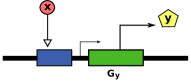
(a) simple gene

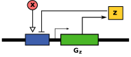
(b) auto-repressed gene

Figure 1: The model. 1(a) Gene $G_{y}$ activity is regulated only by protein $x$. 1(b) The output protein of an auto-repressed gene is regulated by protein $x$ and down regulated by its own product protein.

$x$	abundance of the regulatory input protein
$y$	output abundance of the simple gene
$z$	output abundance of the auto-repressed gene
$\beta$	maximum expression rate for both genes
$\mu$	decay rate of the output proteins
$f(x)$	gene activation function
$K$	threshold of the gene activation function
$l$	Hill coefficient of the gene activation function
$g(z)$	gene auto-repression function
$K_{n}$	threshold of the gene auto-repression function
$x_{L}$	abundance level of the input that leads to low gene expression
$x_{H}$	abundance level of the input that leads to high gene expression
$H$	high abundance level of the output for both the simple and auto-repressed genes
$L$	low abundance level of the output for the simple gene
$L_{n}$	low abundance level of the output for the auto-repressed gene
$m$	relative leak rate, $m=L/H$ or $m=L_{n}/H$
$x_{0},\ y_{0},\ z_{0}$	initial steady state abundance of the specific protein
$x^{*},\ y^{*},\ z^{*}$	new steady state abundance of the specific protein
$y_{\theta},\ z_{\theta}$	fraction $\theta$ of the new steady state abundance
$\tilde{t},\ \tilde{\beta},\ \tilde{T}$	specific parameters when the time is measured in $1/\mu$ (change of variable)
$T_{y}^{LH},\ T_{z}^{LH}$	switching on time
$\ T_{y}^{HL},\ T_{z}^{HL}$	switching off time
$T_{d}^{LH},\ T_{d}^{HL}$	difference between the switching time of the simple gene and the one of the auto-repressed gene
$\sigma^{2}_{y},\ \sigma^{2}_{z}$	variance of the steady state abundance
$\eta_{y},\ \eta_{z}$	normalized variance (noise) of the steady state abundance
$\eta^{\textrm{in}}_{y},\ \eta^{\textrm{in}}_{z}$	intrinsic component of noise
$\eta^{\textrm{up}}_{y},\ \eta^{\textrm{up}}_{z}$	upstream (from input) component of noise
$\eta_{c}^{\textrm{in}},\ \eta_{c}^{\textrm{up}}$	ratio between the noise of the auto-repressed gene and the one of the simple gene

Table 1: Nomenclature

Usually, the equilibrium state (steady-state) and the kinetic behaviour (time evolution) of a system are defined using the differential equation associated to the system (the ODE) (Murray, 2002). In the case of the simple gene, the ODE has the following form

$$\frac{dy(t)}{dt}=\beta f(x)-\mu y(t)$$ (3)

This system is completely determined by the input $x$, which is assumed to change instantaneously between two abundance levels, $x=x_{L}$ and $x=x_{H}$ (Zabet and Chu, 2010; Chu et al., 2011). These two levels of abundances of $x$ will lead to two concentration levels of the output $y$, namely a high concentration state ($y=H$ when $x=x_{H}$) and a low one ($y=L$ when $x=x_{L}$); see Figure 2(a). For convenience, the low state (also called the leak rate) will be denoted as the fraction $m$ from the high state

$$L=mH,\quad m\in[0,1]$$ (4)

where by restricting $m$ to the interval $[0,1]$ it is ensured that $L\leq H$.

Note that Rosenfeld et al. (2002) assumed that the concentration of the output evolved from an initial value of zero ($y_{0}=L=0$) to a new non-zero one ($y^{*}=H>0$), which led to the following limitations: ($i$) they only consider the switching on (or raise) time and ($ii$) they assume that there is no leaky gene expression. The current paper assumes a more general scenario, in which both the initial ($y_{0}$) and the new steady state ($y^{*}$) have positive values ($y_{0}\geq 0$ and $y^{*}\geq 0$) and the system can evolve in both directions, i.e., in the case of switching on, the gene evolves from a low output state ($y_{0}=L$) to high one ($y^{*}=H$), while, in the case of switching off, the gene evolves from a high output state ($y_{0}=H$) to a low one ($y^{*}=L$); see Figure 2(b).

(a) steady state

(b) dynamic behaviour

Figure 2: Steady state and dynamic behaviour of the simple gene. 2(a) The output concentration of gene $G_{y}$ depends on the abundance of the regulatory protein $x$. The activation case was considered. 2(b) The input of the system ($x$) changes instantaneously between a low state $x_{L}$ (corresponding $y=L$) and a high state $x_{H}$ (corresponding to $y=H$). In the case of switching on $y$ evolves from $y_{0}=L$ to $y^{*}=H$, while in the case of switching off $y$ evolves from $y_{0}=H$ to $y^{*}=L$. $t_{r}$ is the response time, which was defined by Rosenfeld et al. (2002) as the time to reach $50\%$ activation. $T_{gene}$ is the time to reach a fraction ($90\%$ in this graph) of the new steady state (Zabet and Chu, 2010).

2.2 Auto-Repressed Gene

A negatively auto-regulated gene is a gene which synthesises a protein that represses its own synthesis; see Figure 1(b). The auto-repressed gene is denoted by $G_{z}$ and this gene synthesises protein $z$. The differential equation that describes this system becomes

$$\frac{dz}{dt}=\beta f(x)g(z)-\mu z$$ (5)

where $g(z)$ is a Hill repression function,

$$g(z)=\gamma\frac{K_{n}^{h}}{K_{n}^{h}+z^{h}}.$$

The auto-repression function, $g(z)$, adds three new parameters, namely: $\gamma$ the maximum contribution of the auto-repression function ($\beta\gamma$ is the maximum production rate), $K_{n}$ the auto-repression threshold and $h$ the auto-repression Hill coefficient. In order to keep the mathematics trackable, this function needs to be brought to a simpler form. First, similarly as in the paper of Rosenfeld et al. (2002), it is assumed that the auto-repression Hill coefficient is $1$. This yields

$$g(z)=\gamma\frac{K_{n}}{K_{n}+z}$$ (6)

Note that bacterial cells can implement auto-repression when the output protein binds to the promoter area of the gene and stops the RNAp molecules to transcribe the gene. In this case and assuming that only monomers auto-regulate the gene, the Hill coefficient of the auto-repression function is $1$ (Chu et al., 2009).

Furthermore, to make the comparison ”fair”, the two systems (the simple gene and the negatively auto-regulated one) will display equal metabolic costs. As previously (Zabet and Chu, 2010; Chu et al., 2011), it is assumed that the metabolic cost of a gene is approximated by the maximum production rate, which represents the pessimistic scenario. This maximal production rate is achieved when $x=x_{H}$, which results in the abundance of the output proteins reaching the maximum value of $y=z=H$. Note that the exact metabolic cost will depend on various additional factors, such as the length of the encoded protein, the average time the gene is active and so on. Nevertheless, these details are irrelevant in the current scenario, where only systems with single genes are considered.

Since the metabolic cost ($\zeta$) is measured as the maximum production rate (when $x=x_{H}$), imposing that the two systems have equal metabolic costs yields

$$\zeta=\beta\cdot f(x_{H})\cdot g(H)=\beta\cdot f(x_{H})$$

which leads to

$$g(z)=\frac{K_{n}+H}{K_{n}+z}$$ (7)

where $\gamma$ was set to $\gamma=(K_{n}+H)/K_{n}$ in order to ensure that the two systems have equal metabolic cost. Hence, the new parameter $\gamma$ was removed from the model.

The steady state abundance levels of the output $y$ which corresponds to the input concentration levels of $x=x_{L}$ and $x=x_{H}$ are computed as follows. First, for $x=x_{H}$, it results from equation (7) that $g(z)=1$ and, thus, the differential equation (5) becomes

$$\frac{dz}{dt}=\beta f(x)-\mu z$$

This yields

$$H_{n}=\frac{\beta}{\mu}f(x_{H})=H$$ (8)

, which led to the same steady state abundance as in the case of the simple gene.

Furthermore, feeding equation (7) into the differential equation (5) and solving at steady state for $x=x_{L}$ leads to only one positive solution:

$$L_{n}=\frac{1}{2}\left(-K_{n}+\sqrt{K_{n}^{2}+4\frac{\beta}{\mu}f(x_{L})\left(K_{n}+H\right)}\right)$$ (9)

The low output state of the negatively auto-regulated gene is denoted by $L_{n}$, as opposed to $L$, the low output state of the simple gene. Since both systems display the same abundance in the high output state, this high output state will be denoted by $H$.

From the form of equations (8) and (9) one can see that the high output state remains constant while changing the strength of the auto-repression, $K_{n}$, but the low state is increased if the auto-repression is strengthened ($K_{n}\searrow\ \Rightarrow\ L_{n}\nearrow$). It can be shown that the low state of the output varies between the following limits

$$\lim_{K_{n}\rightarrow\infty}L_{n} = \frac{\beta}{\mu}f(x_{L})=L$$

$$\lim_{K_{n}\rightarrow 0}L_{n} = \frac{\beta}{\mu}\sqrt{f(x_{L})f(x_{H})}=\sqrt{L\cdot H}=\sqrt{m}\cdot H$$ (10)

Depending on the relationship between $K_{n}$ and $H$, the auto-regulation function (7) can be rewritten in a simpler form. In particular, there are two extreme cases: ($i$) $K_{n}\gg H$ and ($ii$) $K_{n}\ll H$. In the limit of weak auto-repression ($K_{n}\gg H$), the system will be similar to the simple one. This case does not pose any interest, since this paper aims to compare the simple gene to a system that displays different behaviour.

Furthermore, for $K_{n}\ll H$, the auto-repression becomes strong and the auto-regulation function is approximated by

$$g(z)=\frac{K_{n}+H}{K_{n}+z}\approx\frac{H}{z}$$ (11)

Note that the current definition of strong auto-repression is slightly different from the one of Stekel and Jenkins (2008), which considers strong auto-repression in absolute values, i.e., smaller than $<10^{-4}\ \mu M$. The current definition is rather concerned with the relative repression strength ($K_{n}$) compared with the high abundance level of the output species ($H$) and aims to determine a parameter space where the auto-regulation function (7) can be written in a simpler form (11).

In this case, $K_{n}\ll H$, the low output state will be approximated

$$L_{n}\approx\sqrt{m}H$$ (12)

The auto-repression function specified in equation (11) does not contain any of the three additional parameters ($\gamma$, $K_{n}$ and $h$) and, thus, it represents a simpler mathematical formulation of the system. This form of the auto-repression function will be used, in the next section, to compare the two systems (simple gene and auto-repressed one) in both speed and accuracy.

3 Response Time

Generally, one would want to process information as fast as possible, but genes are very slow, in the sense that the time required to turn on/off a gene (the switching time) is of the order of tens of minutes, even for an instant input change. Thus, it is essential to investigate what constrains the speed at which genes function and whether there are any methods to increase this speed.

A common measure of the processing speed of genes is the response time; that is the time required for the output of a gene to reach a new steady state once the input was changed. Note that the regulatory input, $x$, evolves from the initial abundance state $x_{0}$ to the new one $x^{*}$ (switching between $x_{L}$ and $x_{H}$). The input $x$ can either change instantaneously or non-instantaneously and, below, both cases will be considered.

3.1 Instantaneous Change of Input

The time of the simple gene to reach a fraction $\theta$ of the steady state when the input is changed instantaneously was computed previously by Zabet and Chu (2010) as

$$T_{y}=\frac{1}{\mu}\ln\frac{y^{*}-y_{0}}{y^{*}-y_{\theta}}$$ (13)

where $y_{\theta}=y_{0}+(y^{*}-y_{0})\theta$.

In the case of the auto-repressed gene, knowing that the auto-repression function is the one from equation (11), the solution to the differential equation (5) yields

$$z(t)=\sqrt{\frac{\beta}{\mu}f(x)H+\left[(z_{0})^{2}-\frac{\beta}{\mu}f(x)H\right]e^{-2\mu t}}$$ (14)

The time to reach a fraction $\theta$ of the steady state, $z_{\theta}=z_{0}+(z^{*}-z_{0})\theta$, becomes

$$T_{z}=\frac{1}{2\mu}\ln\frac{\frac{\beta}{\mu}f(x)H-\mu^{2}(z_{0})^{2}}{\frac{\beta}{\mu}f(x)H-\mu^{2}(z_{\theta})^{2}}=\frac{1}{2\mu}\ln\frac{(z^{*})^{2}-\mu^{2}(z_{0})^{2}}{(z^{*})^{2}-\mu^{2}(z_{\theta})^{2}}$$ (15)

where the steady state solution for the output protein $z$ was used, $z^{*}=\sqrt{\beta f(x)H/\mu}$.

To make the comparison easier, a change of variable will be performed to the differential equations attached to the two systems, (3) and (5). The time $t$ will be measured in units of $1/\mu$ and this new time is denoted by $\tilde{t}=t/\mu$. The two differential equations become

$$\frac{dy}{d\tilde{t}} = \tilde{\beta}f(x)-y$$ (16)

$$\frac{dz}{d\tilde{t}} = \tilde{\beta}f(x)\frac{H}{z}-z$$ (17)

Recomputing the time to reach a fraction $\theta$ of the steady state yields

$$\tilde{T}_{y} = \ln\frac{y_{0}-y^{*}}{y_{\theta}-y^{*}}$$ (18)

$$\tilde{T}_{z} = \frac{1}{2}\ln\frac{(z^{*})^{2}-(z_{0})^{2}}{(z^{*})^{2}-(z_{\theta})^{2}}$$ (19)

In the case of the simple gene, the switching on and switching off are equal. However, for the auto-repressed gene, these two response times are usually different. The response time of the gene is measured as the maximum between switching on time and switching off time (Zabet et al., 2010).

3.1.1 Switching On

First, the case when the two systems are turned on will be considered, i.e., ($y_{0}=L$, $y^{*}=H$) and ($z_{0}=L_{n}$, $z^{*}=H$). The fraction $\theta$ of the steady state can be written as:

$$y_{\theta} = L+(H-L)\theta=H\left[m+(1-m)\theta\right]$$

$$z_{\theta} = L_{n}+(H-L_{n})\theta=H\left[\sqrt{m}+(1-\sqrt{m})\theta\right]$$ (20)

where the following equations where used $L=m\cdot H$ and $L_{n}=\sqrt{m}\cdot H$

Using equations (18) and (19) the switching on times yield

$$\tilde{T}_{y}^{LH} = \ln{\frac{1}{1-\theta}}$$

$$\tilde{T}_{z}^{LH} = \frac{1}{2}\ln{\frac{1-m}{1-\left[\sqrt{m}+(1-\sqrt{m})\theta\right]^{2}}}$$ (21)

The two times to reach a fraction of the steady state are compared by computing the difference between the two

$$\tilde{T}_{d}^{LH} = \tilde{T}_{y}^{LH}-\tilde{T}_{z}^{LH}$$

$$= \frac{1}{2}\ln{\left[\frac{1}{(1-\theta)^{2}}\frac{1-\left[\sqrt{m}+(1-\sqrt{m})\theta\right]^{2}}{1-m}\right]}$$

$$= \frac{1}{2}\ln{\frac{1-m-2\sqrt{m}\theta+2m\theta-\theta^{2}+2\sqrt{m}\theta^{2}-m\theta^{2}}{1-m-2\theta+2m\theta+\theta^{2}-m\theta^{2}}}$$

This time difference is positive (and consequently negative auto-regulation speeds up the switching on) when the fraction in the logarithm is higher than or equal to $1$, which takes place when

$$\theta(1-\theta)(1-\sqrt{m})\geq 0$$

This is true for any $\theta,m\in[0,1]$. Hence, negative auto-regulation always speeds up the switching on time compared with the simple gene. Figure 3(a) confirms this result and shows that higher fractions $\theta$ of the steady states display better increase in speed that lower ones.

\psfrag{timedifference}{$\tilde{T}_{d}^{LH}$}\includegraphics[scale={0.82}]{graph_time_nar_LH_lines.eps}

(a) switching on

\psfrag{timedifference}{$\tilde{T}_{d}^{LH}$}\includegraphics[scale={0.82}]{graph_time_nar_HL_lines.eps}

(b) switching off

Figure 3: Negative auto-regulation enhances the switching speed. For any combination $(\theta,m)\in[0,1]^{2}$ the difference between the switching time of the simple gene and of the auto-repressed gene is positive. This means that the auto-repressed gene is faster than the simple gene. Note that this time difference is measured in $1/\mu$ and, thus, the actual time enhancement scales by $1/\mu$, i.e., $T_{d}^{LH}=\tilde{T}_{d}^{LH}/\mu$.

In the special case of no leak rate (the optimum configuration for noise), $L=0$ and $L_{n}=0$, the time gain reduces to

$$\tilde{T}_{d}^{LH}=\frac{1}{2}\ln{\frac{1+\theta}{1-\theta}}$$ (22)

which is positive as long as $\theta>0$.

3.1.2 Switching Off

When the gene is turned off, ($y_{0}=H$, $y^{*}=L$) and ($z_{0}=H$, $z^{*}=L_{n}$), the output states ($H$, $L$ and $L_{n}$) remain the same as the ones for switching on, but the fractions $\theta$ of the steady state become

$$y_{\theta} = H+(L-H)\theta=H\left[1-(1-m)\theta\right]$$

$$z_{\theta} = H+(L_{n}-H)\theta=H\left[1-(1-\sqrt{m})\theta\right]$$ (23)

From equations (18) and (19) one can compute the switching off time as

$$\tilde{T}_{y}^{HL} = \ln{\frac{1}{1-\theta}}$$

$$\tilde{T}_{z}^{HL} = \frac{1}{2}\ln{\frac{1-m}{\left[1-(1-\sqrt{m})\theta\right]^{2}-m}}$$ (24)

The difference in time between $\tilde{T}^{HL}$ and $\tilde{T}^{HL}$ yields

$$\tilde{T}_{d}^{HL} = \tilde{T}_{y}^{HL}-\tilde{T}_{z}^{HL}$$

$$= \frac{1}{2}\ln{\left[\frac{1}{(1-\theta)^{2}}\frac{\left[1-(1-\sqrt{m})\theta\right]^{2}-m}{1-m}\right]}$$

$$= \frac{1}{2}\ln{\frac{1-2\theta+2\sqrt{m}\theta+\theta^{2}-2\sqrt{m}\theta^{2}+m\theta^{2}-m}{1-m-2\theta+2m\theta+\theta^{2}-m\theta^{2}}}$$

Analogously, as in the case of switching on, one can determine whether the time difference is positive by verifying if the fraction in the logarithm is higher than or equal to $1$, which reduces to

$$\theta\sqrt{m}(1-\theta)(1-\sqrt{m})\geq 0$$

This means that $\tilde{T}_{d}^{HL}$ is always positive and the time to switch off an auto-repressed gene is at most equal to the time to switch off the simple gene. Figure 3(b) confirms these results.

In the case of vanishing leak rates $m=L=L_{n}=0$, the time difference between the two systems becomes zero

$$\tilde{T}_{d}^{HL}=\frac{1}{2}\ln{\frac{(1-\theta)^{2}}{(1-\theta)^{2}}}=0$$ (25)

Thus, for vanishing leak rates, the auto-repressed gene turns on faster compared with the simple gene, but has an equal speed when turning off. Vanishing leak rates are optimal in terms of noise and require $f(x_{L})$ to be zero. This is usually difficult to achieve. For repressor genes, the gene can be turn off completely if either the Hill coefficient or $x_{L}$ have high values, which comes at a high metabolic cost (Zabet and Chu, 2010). Even for activator genes, having a gene completely turned off can be very difficult to achieve, i.e., the regulator molecule would need to be totally absent and the affinity of RNAp for the non activated promoter should be zero. Putting all together, in the case of non-vanishing leak rates (sub-optimal in terms of noise), the negative auto-regulation speeds the switching in both directions (on and off).

3.2 Non-Instantaneous Change of Input

The assumption that $x$ changes instantaneously between $x_{L}$ and $x_{H}$ will be relaxed now. In the case of non-instantaneous input change, the solution of the differential equations (3) and (5) can only be computed numerically. For very fast, but non-instantaneous input change, one expects the behaviour to be similar to the one predicted by the instantaneous input change. Figure 4(a) confirms that the difference between the switching off time of the simple gene and the one of the auto-repressed gene is always positive.

(a) Fast non-instantaneous input change

(b) Slow non-instantaneous input change

Figure 4: Non-instantaneous input change and speed. The following set of parameters have been used: $\theta=0.9$, $l=2$ and $x_{H}=0.9\ \mu M$. $x_{L}$ was varied in the interval $x_{L}\in[0.0,0.2]$ and, thus, $m$ varied accordingly. The regulation threshold is selected so that the threshold resides midway between the two states of the input $K=0.5\cdot(x_{H}+x_{L})$ and the synthesis rate so that the cost remains fixed to $\zeta=1.2\ \mu Mmin^{-1}$. Both graphs consider the activation case. 4(a) The input is assumed to change ten times faster than the output, i.e., $\mu=1\ min^{-1}$ and $\mu_{x}=10\ min^{-1}$. 4(b) The input is assumed to change at the same speed as the output, i.e., $\mu=1\ min^{-1}$ and $\mu_{x}=1\ min^{-1}$

Usually, it is assumed that the input and the output are affected by the same decay rate (dilution) and, thus, they change at a similar speed. The numerical analysis reveals that for most of the parameter space the relationship between switching times (the signs of $T_{d}^{LH}$ and $T_{d}^{HL}$) is conserved (see Figure 4(b)). However, for no or very small leak rate ($m\leq 0.0002$ in Figure 4(b)) the switching off time seems to be increased by negative auto-regulation. This suggests that negative auto-regulation is beneficial for speed but only for non-vanishing leak rates of the output gene.

4 Noise

Gene expression is affected by noise (Spudich and Koshland Jr., 1976; Arkin et al., 1998; Elowitz et al., 2002). This noise is a consequence of the fact that genes have low copy numbers and that they are slowly expressed (Kaern et al., 2005). In the context of genes as computational units, this output noise is undesirable because it makes difficult the assessment of the output of the gene as either low or high.

At steady state one can compute the variance of the output species $y$ of the simple gene as (Paulsson, 2004; Shibata and Fujimoto, 2005; van Kampen, 2007):

$$\sigma_{y}^{2}=y+\left[\beta f^{\prime}(x)\tau\right]^{2}\frac{1}{1+\tau/\tau_{x}}x$$ (26)

Usually, gene expression is modelled as a three steps process (regulation, transcription and translation), but here it is modelled as a one step process. Consequently, the noise produced by regulation and translation steps is ignored and the output noise stems mainly from transcription. Nevertheless, this assumption is often valid as shown both theoretically and experimentally (Bar-Even et al., 2006; Newman et al., 2006).

As proposed previously (Zabet and Chu, 2010; Zabet et al., 2010; Chu et al., 2011), the noise will be measured by computing the variance in the high state, $y=H$, normalized by the square of the signal strength (the difference between the high and the low state), $\eta_{y}=\sigma_{y}^{2}/(H-L)^{2}=\sigma_{y}^{2}/[H^{2}(1-m)^{2}]$.

$$\eta_{y} = \overbrace{\frac{1}{H(1-m)^{2}}}^{\eta_{y}^{\textrm{in}}}+\overbrace{\left[\frac{f^{\prime}(x_{H})}{f(x_{H})(1-m)}\right]^{2}\frac{1}{1+\tau/\tau_{x}}x_{H}}^{\eta_{y}^{\textrm{up}}}$$ (27)

$$= \frac{1}{(1-m)^{2}}\left[\frac{1}{H}+\left(\frac{f^{\prime}(x_{H})}{f(x_{H})}\right)^{2}\frac{1}{1+\tau/\tau_{x}}x_{H}\right]$$

The noise consists of two components: the intrinsic noise, $\eta^{\textrm{in}}$, (generated by the randomness of the birth/death process) and the upstream (or extrinsic) noise, $\eta^{\textrm{up}}$, (propagated from the upstream component) (Elowitz et al., 2002; Swain et al., 2002; Pedraza and van Oudenaarden, 2005).

In the case of the auto-repressed gene, the steady state variance of the species $z$ yields (Paulsson, 2004; Shibata and Fujimoto, 2005; van Kampen, 2007)

$$\sigma_{z}^{2}=\frac{z}{1+\tau\beta f(x)H/z^{2}}+\left[\frac{\tau\beta f^{\prime}(x)H/z}{\tau\beta f(x)H/z^{2}+1}\right]^{2}\frac{1}{1+\frac{\tau}{\tau_{x}}\frac{1}{1+\tau\beta f(x)H/z^{2}}}x$$

Then, the noise of the auto-repressed gene (the variance in the high state normalised by the square of the signal strength) becomes

$$\eta_{z} = \overbrace{\frac{1}{H2(1-\sqrt{m})^{2}}}^{\eta_{z}^{\textrm{in}}}+\overbrace{\left[\frac{f^{\prime}(x_{H})}{f(x_{H})\sqrt{2}(1-\sqrt{m})^{2}}\right]^{2}\frac{1}{2+\tau/\tau_{x}}x_{H}}^{\eta_{z}^{\textrm{up}}}$$ (28)

$$= \frac{1}{2(1-\sqrt{m})^{2}}\left[\frac{1}{H}+\left(\frac{f^{\prime}(x_{H})}{f(x_{H})}\right)^{2}\frac{1}{2+\tau/\tau_{x}}x_{H}\right]$$

where the following two steady state equations were used: $\beta f(x_{H})\tau/H=1$ and $\tau\beta/H=f(x_{H})$.

The reliability of the analytical method for noise was validated previously by a series of stochastic simulations. The results confirmed that LNA works well for both the simple gene (Zabet and Chu, 2010) and the auto-repressed one (Thattai and van Oudenaarden, 2001; Hayot and Jayaprakash, 2004; Stekel and Jenkins, 2008). However, for extremely strong auto-repression values ($K_{n}<10^{-4}\ \mu M$), the analytical method underestimates the simulation results (Stekel and Jenkins, 2008). In this context, it is worthwhile noting that Zhang et al. (2009) showed that, although the LNA underestimates the actual value of the noise in the auto-repressed gene, it still captures the dependence of noise on the parameters of the system.

The noise of the two systems (the simple and the auto-repressed gene) is compared by analysing the ratio for each component of the noise (intrinsic and upstream).

$$\eta_{c}^{\textrm{in}}=\frac{\eta_{z}^{\textrm{in}}}{\eta_{y}^{\textrm{in}}}=\frac{(1+\sqrt{m})^{2}}{2}\quad\textrm{and}\quad\eta_{c}^{\textrm{up}}=\frac{\eta_{z}^{\textrm{up}}}{\eta_{y}^{\textrm{up}}}=\frac{(1+\sqrt{m})^{2}}{2}\frac{1+\tau/\tau_{x}}{2+\tau/\tau_{x}}$$ (29)

Examining the first equation, one can notice that, for low leak rates ($m\leq 0.17$), the intrinsic component of the noise is not amplified by negative feedback.

$$\eta_{c}^{\textrm{in}}=\frac{(1+\sqrt{m})^{2}}{2}\leq 1\ \Rightarrow\ m\leq(\sqrt{2}-1)^{2}\approx 0.17$$

Furthermore, the fraction $(1+\tau_{y}/\tau_{x})/(2+\tau_{y}/\tau_{x})$ can never be higher than one. This yields

$$\eta_{c}^{\textrm{up}}\leq\frac{(1+\sqrt{m})^{2}}{2}\Rightarrow m\lesssim 0.17$$

Overall, for low leak rates, the intrinsic and the upstream components of the noise are reduced.

Figure 5: The leak rate influences the noise levels of negative auto-regulation. Increasing the leak rate reduces the accuracy. The following set of parameters was used: $\theta=0.9$, $\mu=1min^{-1}$, $x_{H}=0.9\ \mu M$, $K_{n}=0.01\ \mu M$ and $V=8\cdot 10^{-16}\ l$. $\beta$ was selected so that the cost remains fixed to $\zeta=1.2\ \mu Mmin^{-1}$ and $K$ so that the threshold resides at the midpoint between the low and the high state of the input, $K=0.5\cdot(x_{H}+x_{L})$. The noise generated by $x$ is assumed to be Poissonian. The gene is activated by a regulatory input $x$.

Figure 5 confirms that, for low levels of leak rate, negative feedback enhances accuracy. This in conjunction with the fact that negative feedback increases speed for high leak rates suggest that there is a trade-off between speed and accuracy, in the sense that for lower leak rates the auto-repressed gene is more accurate than the simple gene while for higher leak rates the auto-repressed gene becomes faster. Nevertheless, these results indicate that there is a range of values for the leak rate for which the auto-repressed gene is both faster and more accurate compared to the simple one.

A gene with negative feedback and low but non zero leak rate will display less noise ($m<0.1$ in Figure 5) and shorter response time ($m>0$ in Figure 3) compared to the optimal configuration of the simple gene with an equivalent metabolic cost. This shows that negative feedback is able to improve the performance of a gene beyond the one of the zero leak rate configuration and without increasing the metabolic cost.

5 Speed-Accuracy Trade-offs

Recently, Zabet and Chu (2010) showed that the processing speed and accuracy of genes are connected, in the sense that there is a trade-off between speed and accuracy, which is controlled by the decay rate. Figure 6 confirms the existence of this trade-off also in the case of the auto-repressed gene. Furthermore, the graph confirms that for low leak rates the auto-repressed gene displays a better trade-off curve compared to the simple one; see Figure 6(a). Note that not only the metabolic cost is fixed along the curve, but also the two curves display equal costs. In the case of high leak rate, the auto-repressed gene is still faster than the simple one, but this time the noise in the former is higher than the one in the latter.

(a) low leak rate

(b) high leak rate

Figure 6: Speed-accuracy trade-off curves for instantaneous change of input. The following set of parameters was used: $\theta=0.9$, $x_{H}=0.9\ \mu M$, $K=0.7\ \mu M$, $K_{n}=0.01\ \mu M$ and $V=8\cdot 10^{-16}\ l$. $\beta$ was selected so that the cost remains fixed to $\zeta=1.2\mu Mmin^{-1}$ and the decay rate $\mu$ was varied in the interval $\mu\in[0.5,1.5]\ min^{-1}$. $G_{y}$ and $G_{z}$ are activator genes. Similar results can be obtained when the genes are repressed by the regulatory input $x$. The noise generated by $x$ is assumed to be Poissonian. Two cases were considered: 6(a) $x_{L}=0.05\ \mu M$ and 6(b) $x_{L}=0.30\ \mu M$

Figure 6 shows that for low (but non-zero) leak rate it is always better for the gene to display negative feedback, i.e., the auto-repressed gene is both faster and more accurate than the simple one. However, for high leak rates, the cell has to choose between being fast or more accurate, by selecting whether it has negative feedback or not. This result reveals a new speed-accuracy trade-off, which is not controlled by a parameter of the system (as previously identified), but rather by the architecture of the system.

For zero leak rate, both auto-repressed and simple genes display the lowest noise configurations and this is denoted by $m=m_{\eta}$. It is worthwhile noting that, by increasing the leak rate, the speed gain is increased while the accuracy gain is reduced; see Figure 7. However, the increase in speed is achieved up to a certain maximum speed ($m_{T}$), above which the speed cannot be increased further by negative feedback. This indicates that there is no advantage in having leak rates higher than this optimal point in speed, while for any leak rate in the interval $m\in[m_{T},m_{\eta}]$ there is a speed-accuracy trade-off.

(a) instantaneous change of input

(b) exponential change of input

Figure 7: Speed-accuracy trade-off curves and leak rate. The following set of parameters was used: $\theta=0.9$, $\mu=1\ min^{-1}$, $\mu_{x}=1\ min^{-1}$, $x_{H}=0.9\ \mu M$, $K=0.7\ \mu M$, $K_{n}=0.01\ \mu M$ and $V=8\cdot 10^{-16}\ l$. The noise generated by $x$ is assumed to be Poissonian. $\beta$ was selected so that the cost remains fixed to $\zeta=1.2\mu Mmin^{-1}$ and the leak rate $m$ was varied in the interval $m\in[0.0,0.5]$. $G_{y}$ and $G_{z}$ are activator genes.

6 Discussion

Negative auto-regulation was suggested as an alternative approach to reduce the response time of a single gene. Rosenfeld et al. (2002) showed theoretically that negative auto-regulation can speed up only the turn on response time, i.e., the turn on time of a negatively auto-regulated gene is five times smaller than the one of a simple gene. In the context of genes as computational units, the direction of switching is not important in the sense that the system needs to turn both on and off as fast as possible. One of the assumptions of Rosenfeld et al. (2002) is that the auto-repressed gene does not have a leaky expression, which is not always biologically plausible. In this contribution, it is shown that, in the case of leaky gene expression, auto-repressed genes are always faster compared to the simple ones in both turning on and off; see Figures 3 and 4.

Furthermore, several theoretical studies showed that negative auto-regulation reduces the output noise (Thattai and van Oudenaarden, 2001; Paulsson, 2004; Shahrezaei et al., 2008; Hornung and Barkai, 2008; Bruggeman et al., 2009). These results were obtained without comparing two systems with equal cost and, in fact, the negatively auto-regulated system displays a lower metabolic cost. Nevertheless, several studies (Paulsson and Ehrenberg, 2000; Stekel and Jenkins, 2008; Zhang et al., 2009) compared the noise in the simple and auto-repressed gene under the assumption of fixed average number of molecules at steady state, which, in their settings, could be thought as the metabolic cost. A better measure of metabolic cost is the energy consumption per time unit and the scaling properties of this are well given by the protein production rate.

Recently, Chu et al. (2011) found that negative feedback can reduce output noise in a gene cascade under the assumption of fixed production rate. However, the study of Chu et al. (2011) did not identify what parameter controls whether the auto-repressed gene has lower or higher noise compared to the simple one. This current paper considers the case of a single gene (not a cascade) and compares the auto-repressed gene to a simple one by keeping the metabolic cost (maximum production rate) fixed. The results revealed that the leak expression rate plays a crucial role for the output noise, in the sense that, for low leak rates, the auto-repressed gene is less noisier than the simple one, while, for high leak rates, the auto-repressed gene becomes noisier; see Figure 5. This result can be explained by the fact that increasing the leak expression rate reduces the signal strength and, consequently, it reduces the normalisation term of the noise, $(H-L)^{2}$. The reduction in the signal strength is more pronounced in the case of the auto-repressed gene than in the case of the simple gene, because the low state increases faster in the former compared to the latter. Thus, negative feedback increases the sensitivity of noise to the leak expression rate. Note, however, that these analytical results of noise cannot be extended automatically to very strongly auto-repressed genes ($K_{n}<10^{-4}\ \mu M$), where the Linear Noise Approximation seems to fail to represent accurately the noise of the system (Stekel and Jenkins, 2008).

Previously, Zabet and Chu (2010) showed that the speed-accuracy properties of a gene can be enhanced by reducing the leak rate, which comes at an undesirable increase in the metabolic cost. Here, it is proved that negative feedback can further enhance the speed-accuracy properties of genes without increasing the metabolic cost, by actually exploiting the non-zero leak rate of genes; see Figures 3 and 5.

Hence, negative feedback is able to enhance the performance of a gene and this can explain why a high proportion of the bacterial genes display this mechanism. For example, in E.Coli, $40\%$ of the genes are auto-repressed (Austin et al., 2006). Nevertheless, one question that still needs to be addressed is why only $40\%$ of the genes are negatively auto-regulated and not a higher proportion. One possible answer to this question is that for high leak rates the negative feedback only enhances speed, while at the same time reduces accuracy; see Figure 6(b). Thus, a system that displays higher leak rates has to choose between being faster or being more accurate, in the sense that the simple gene is the most accurate system, while the auto-repressed one is the fastest. It might be the case that, sometimes, it is more important for the system to be more accurate that faster, while other times to be faster than more accurate.

Finally, the results revealed that the leak rate controls a speed-accuracy trade-off in a negatively auto-regulated gene. Particularly, there are two specific leak rate values: one which optimises the system in terms of accuracy ($m_{\eta}=0$) and another which optimises the system in speed ($m_{T}>0$); see Figure 7. Increasing the leak rate above $m_{T}$ results in a system that is not faster than the optimal system in speed, but which has higher noise levels. This means that the leak rate determines two speed-accuracy trade-off curves, namely: ($i$) $m\in[0,m_{T}]$ where the system can be optimised in speed or accuracy and ($ii$) $m\in[m_{T},1]$ where the system is always suboptimal in terms of noise and speed compared to the first case. Hence, the optimal parameter set for an auto-repressed gene consists of leak rates smaller than or equal to $m_{T}$, while for higher leak rates the auto-repressed gene becomes suboptimal.

To sum up, negative feedback further introduces additional speed-accuracy trade-offs for genes as information processors. These trade-offs manifest through either sets of parameters (such as leak rate) or the actual architecture of the system (as either with or without feedback). Various configuration of parameters and architectures that are encountered in today’s living organisms are results of long time evolution towards an optimal design.

7 Acknowledgements

The author would like to thank Dr Dominique F.Chu, Professor Andrew N.W. Hone, Dr Boris Adryan and the anonymus reviewers for useful comments which lead to improvements of the manuscript and Felicia Dana Zabet for proofreading the manuscript.

References

- Ackers et al. (1982) Ackers, G. K., Johnson, A. D., Shea, M. A., 1982. Quantitative model for gene regulation by lambda phage repressor. PNAS 79, 1129–1133.
- Akashi and Gojobori (2002) Akashi, H., Gojobori, T., 2002. Metabolic efficiency and amino acid composition in the proteomes of escherichia coli and bacillus subtilis. PNAS 99 (6), 3695–3700.
- Alon (2007a) Alon, U., 2007a. An Introduction To System Biology. Design Principles of Biological Circuits. Chapman & Hall/CRC Mathematical and Computational Biology Series.
- Alon (2007b) Alon, U., 2007b. Network motifs: theory and experimental approaches. Nature Reviews Genetics 8, 450–461.
- Arkin et al. (1998) Arkin, A., Ross, J., McAdams, H. H., 1998. Stochastic kinetic analysis of developmental pathway bifurcation in phage l-infected escherichia coli cells. Genetics 149, 1633–1648.
- Austin et al. (2006) Austin, D. W., Allen, M. S., McCollum, J. M., Dar, R. D., Wilgus, J. R., Sayler, G. S., Samatova, N. F., Cox, C. D., Simpson, M. L., 2006. Gene network shaping of inherent noise spectra. Nature 439 (2), 608–611.
- Bar-Even et al. (2006) Bar-Even, A., Paulsson, J., Maheshri, N., Carmi, M., O’Shea, E., Pilpel, Y., Barkai, N., 2006. Noise in protein expression scales with natural protein abundance. Nature Genetics 38 (6), 636–643.
- Becskei and Serrano (2000) Becskei, A., Serrano, L., 2000. Engineering stability in gene networks by autoregulation. Nature 405, 590–593.
- Bennett (1973) Bennett, C. H., 1973. Logical reversibility of computation. IBM Journal of Research and Development 17 (6), 525–532.
- Bennett (1982) Bennett, C. H., 1982. The thermodynamics of computation – a review. International Journal of Theoretical Physics 21 (12), 905–940.
- Bintu et al. (2005) Bintu, L., Buchler, N. E., Garcia, H. G., Gerland, U., Hwa, T., Kondev, J., Phillips, R., 2005. Transcriptional regulation by the numbers: models. Current Opinion in Genetics and Development 15, 116–124.
- Bruggeman et al. (2009) Bruggeman, F. J., Blüthgen, N., Westerhoff, H. V., 2009. Noise management by molecular networks. PLoS Computational Biology 5 (9), e1000506.
- Buchler et al. (2003) Buchler, N. E., Gerland, U., Hwa, T., 2003. On schemes of combinatorial transcription logic. PNAS 100 (9), 5136–5141.
- Chu et al. (2009) Chu, D., Zabet, N. R., Mitavskiy, B., 2009. Models of transcription factor binding: Sensitivity of activation functions to model assumptions. Journal of Theoretical Biology 257 (3), 419–429.
- Chu et al. (2011) Chu, D. F., Zabet, N. R., Hone, A. N. W., 2011. Optimal parameter settings for information processing in gene regulatory networks. BioSystems 104 (2-3), 99–108.
- Elowitz et al. (2002) Elowitz, M. B., Levine, A. J., Siggia, E. D., Swain, P. S., 2002. Stochastic gene expression in a single cell. Science 297 (5584), 1183–1186.
- Fernando et al. (2009) Fernando, C. T., Liekens, A. M., Bingle, L. E., Beck, C., Lenser, T., Stekel, D. J., Rowe, J. E., 2009. Molecular circuits for associative learning in single-celled organisms. J. R. Soc. Interface 6 (34), 463–469.
- Hayot and Jayaprakash (2004) Hayot, F., Jayaprakash, C., 2004. The linear noise approximation for molecular fluctuations within cells. Physical Biology 1, 205–210.
- Hooshangi et al. (2005) Hooshangi, S., Thiberge, S., Weiss, R., 2005. Ultrasensitivity and noise propagation in a synthetic transcriptional cascade. PNAS 102 (10), 3581–3586.
- Hornung and Barkai (2008) Hornung, G., Barkai, N., 2008. Noise propagation and signaling sensitivity in biological networks: A role for positive feedback. PLoS Computational Biology 4 (1), 0055–0061.
- Isaacs et al. (2005) Isaacs, F. J., Blake, W. J., Collins, J. J., 2005. Signal processing in single cells. Science 307 (5717), 1886–1888.
- Kaern et al. (2005) Kaern, M., Elston, T. C., Blake, W. J., Collins, J. J., 2005. Stochasticity in gene expression: from theories to phenotypes. Nature Reviews Genetics 6, 451–464.
- Lei (2009) Lei, J., 2009. Stochasticity in single gene expression with both intrinsic noise and fluctuation in kinetic parameters. Journal of Theoretical Biology 256, 485 – 492.
- Lloyd (2000) Lloyd, S., 2000. Ultimate physical limits to computation. Nature 406, 1047–1054.
- Mayo et al. (2006) Mayo, A. E., Setty, Y., Shavit, S., Zaslaver, A., Alon, U., 2006. Plasticity of the cis-regulatory input function of a gene. PLOS Biology 4 (4), e45.
- Mehta et al. (2008) Mehta, P., Mukhopadhyay, R., Wingreen, N. S., 2008. Exponential sensitivity of noise-driven switching in genetic networks. Physical Biology 5.
- Murray (2002) Murray, J. D., 2002. Mathematical Biology I. An Introduction. Springer.
- Newman et al. (2006) Newman, J. R. S., Ghaemmaghami, S., Ihmels, J., Breslow, D. K., Noble, M., DeRisi, J. L., Weissman, J. S., 2006. Single-cell proteomic analysis of s. cerevisiae reveals the architecture of biological noise. Nature 441, 840–846.
- Paulsson (2004) Paulsson, J., 2004. Summing up the noise in gene networks. Nature 427, 415–418.
- Paulsson and Ehrenberg (2000) Paulsson, J., Ehrenberg, M., 2000. Random signal fluctuations can reduce random fluctuations in regulated components of chemical regulatory networks. Physical Review Letters 84 (23), 5447–5450.
- Pedraza and van Oudenaarden (2005) Pedraza, J. M., van Oudenaarden, A., 2005. Noise propagation in gene networks. Science 307, 1965–1969.
- Rosenfeld et al. (2002) Rosenfeld, N., Elowitz, M. B., Alon, U., 2002. Negative autoregulation speeds the response times of transcription networks. Journal of Molecular Biology 323, 785–793.
- Rosenfeld et al. (2005) Rosenfeld, N., Young, J. W., Alon, U., Swain, P. S., Elowitz, M. B., 2005. Gene regulation at the single-cell level. Science 307 (5717), 1962–1965.
- Savageau (1974) Savageau, M. A., 1974. Comparison of classical and autogenous systems of regulation in inducible operons. Nature 252 (5484), 546–549.
- Setty et al. (2003) Setty, Y., Mayo, A. E., Surette, M. G., Alon, U., 2003. Detailed map of a cis-regulatory input function. PNAS 100 (13), 7702–7707.
- Shahrezaei et al. (2008) Shahrezaei, V., Ollivier, J. F., Swain, P. S., 2008. Colored extrinsic fluctuations and stochastic gene expression. Molecular Systems Biology 4 (196).
- Shen-Orr et al. (2002) Shen-Orr, S. S., Milo, R., Mangan, S., Alon, U., 2002. Network motifs in the transcriptional regulation network of escherichia coli. Nature Genetics 31, 64–68.
- Shibata and Fujimoto (2005) Shibata, T., Fujimoto, K., 2005. Noisy signal amplification in ultrasensitive signal transduction. PNAS 102 (2), 331–336.
- Spudich and Koshland Jr. (1976) Spudich, J. L., Koshland Jr., D. E., 1976. Non-genetic individuality: chance in the single cell. Nature 262, 467–471.
- Stekel and Jenkins (2008) Stekel, D. J., Jenkins, D. J., 2008. Strong negative self regulation of prokaryotic transcription factors increases the intrinsic noise of protein expression. BMC Systems Biology 2 (6).
- Stojanovic and Stefanovic (2003) Stojanovic, M. N., Stefanovic, D., 2003. A deoxyribozyme-based molecular automaton. Nature Biotechnology 21 (9), 1069–1074.
- Swain et al. (2002) Swain, P. S., Elowitz, M. B., Siggia, E. D., 2002. Intrinsic and extrinsic contributions to stochasticity in gene expression. PNAS 99 (20), 12795–12800.
- Tan et al. (2007) Tan, C., Reza, F., You, L., 2007. Noise-limited frequency signal transmission in gene circuits. Biophysical Journal 93, 3753–3761.
- Thattai and van Oudenaarden (2001) Thattai, M., van Oudenaarden, A., 2001. Intrinsic noise in gene regulatory networks. PNAS 98 (15), 8614–8619.
- Thieffry et al. (1998) Thieffry, D., Huerta, A. M., Perez-Rueda, E., Collado-Vides, J., 1998. From specific gene regulation to genomic networks: a global analysis of transcriptional regulation in escherichia coli. BioEssays 20 (5), 433–440.
- van Kampen (2007) van Kampen, N. G., 2007. Stochastic processes in physics and chemistry, Third Edition (North-Holland Personal Library), 3rd Edition. North Holland.
- Wang et al. (2010) Wang, L., Xin, J., Nie, Q., 2010. A critical quantity for noise attenuation in feedback systems. PLoS Computational Biology 6 (4), e1000764.
- Weiss et al. (2003) Weiss, R., Basu, S., Hooshangi, S., Kalmbach, A., Karig, D., Mehreja, R., Netravali, I., 2003. Genetic circuit building blocks for cellular computation, communications, and signal processing. Natural Computing 2, 47–84.
- Yokobayashi et al. (2002) Yokobayashi, Y., Weiss, R., Arnold, F. H., 2002. Directed evolution of a genetic circuit. PNAS 99 (26), 16587–16591.
- Zabet (2010) Zabet, N. R., 2010. Towards modular, scalable and optimal design of transcriptional logic systems. Ph.D. thesis, School of Computing, University of Kent, UK.
- Zabet and Chu (2010) Zabet, N. R., Chu, D. F., 2010. Computational limits to binary genes. Journal of the Royal Society Interface 7, 945–954.
- Zabet et al. (2010) Zabet, N. R., Hone, A. N. W., Chu, D. F., 19-23 August 2010. Design principles of transcriptional logic circuits. In: Artificial Life XII: Proceedings of the 12th International Conference on the Synthesis and Simulation of Living Systems. MIT Press, Odense, Denmark.
- Zhang et al. (2009) Zhang, J., Yuan, Z., Zhou, T., 2009. Physical limits of feedback noise-suppression in biological networks. Physical Biology 6 (4), 046009.