Mixing of spherical and spheroidal modes in perturbed Kerr black holes

Abstract

The angular dependence of the gravitational radiation emitted in compact binary mergers and gravitational collapse is usually separated using spin-weighted spherical harmonics ${}_{s}Y_{\ell m}$ of spin weight $s$, that reduce to the ordinary spherical harmonics $Y_{\ell m}$ when $s=0$. Teukolsky first showed that the perturbations of the Kerr black hole that may be produced as a result of these events are separable in terms of a different set of angular functions: the spin-weighted spheroidal harmonics ${}_{s}S_{\ell mn}$, where $n$ denotes the “overtone index” of the corresponding Kerr quasinormal mode frequency $\omega_{\ell mn}$. In this paper we compute the complex-valued scalar products of the ${}_{s}S_{\ell mn}$’s with the ${}_{s}Y_{\ell m}$’s (“spherical-spheroidal mixing coefficients”) and with themselves (“spheroidal-spheroidal mixing coefficients”) as functions of the dimensionless Kerr parameter $j$. Tables of these coefficients and analytical fits of their dependence on $j$ are available online for use in gravitational-wave source modeling and in other applications of black-hole perturbation theory.

I Introduction

Various angular functions, including scalar, vector, and tensor spherical harmonics, are used to perform separation of variables in the general relativity literature. These functions include the Regge-Wheeler harmonics, the symmetric, trace-free tensors of Sachs and Pirani, the Newman-Penrose spin-weighted spherical harmonics, and the Mathews-Zerilli Clebsch-Gordan-coupled harmonics. An excellent review article by Thorne Thorne (1980) lists all of these functions and discusses their mutual relations.

The spin-weighted spherical harmonics ${}_{s}Y_{\ell m}$ Newman and Penrose (1966); Goldberg et al. (1967) are most commonly used to separate the angular dependence of the gravitational radiation emitted as a result of compact binary mergers and gravitational collapse in numerical relativity simulations. Unfortunately, the ${}_{s}Y_{\ell m}$’s are not ideal to study the perturbations of the rotating Kerr black holes of mass $M$ and dimensionless angular momentum $j\equiv a/M$ that may be formed as a result of compact binary mergers or gravitational collapse (here and below $a$ is the usual Kerr parameter, and we use geometrical units: $G=c=1$).

Teukolsky Teukolsky (1973); Press and Teukolsky (1973) first realized that the radiation produced by perturbed Kerr black holes is most conveniently studied using a different set of angular functions: the spin-weighted spheroidal harmonics ${}_{s}S_{\ell m}(a\omega)$ (henceforth SWSHs). The differential equation defining these functions is a generalized spheroidal wave equation Leaver (1986), and it results from separating variables in the partial differential equations describing the propagation of a spin-$s$ field in a rotating (Kerr) black hole background. If we use the Kinnersley tetrad and Boyer-Lindquist coordinates $(t,\,r,\,\theta,\,\phi)$, we assume a time dependence of the form $e^{-{\rm i}\omega t}$ and a $\phi$-dependence of the form $e^{{\rm i}m\phi}$, the SWSHs satisfy the equation Teukolsky (1973); Leaver (1985)

$$\left[(1-x^{2}){}_{s}S_{\ell m,x}\right]_{,x}$$

$$+ \left[(cx)^{2}-2csx+s+{}_{s}A_{\ell m}-{(m+sx)^{2}\over 1-x^{2}}\right]{}_{s}S_{\ell m}=0\,,$$

where $x\equiv\cos\theta$, $c\equiv a\omega$ and $\theta$ is the Boyer-Lindquist polar angle. The angular separation constant ${}_{s}A_{\ell m}$ is, in general, complex. The spin-weight parameter takes on the values $s=0,\pm 1/2,\pm 1,\pm 2$ for massless scalar, spinor, vector and tensor perturbations, respectively.

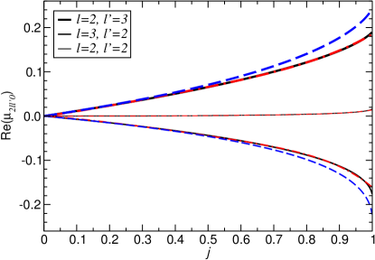
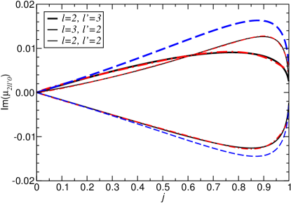
Figure 1: Real (left panel) and imaginary part (right panel) of the spherical-spheroidal mixing coefficients $\mu_{m\ell\ell^{\prime}n^{\prime}}$ for $m=2$, $n^{\prime}=0$. Here we consider the dominant multipoles ($\ell=2,\,\ell^{\prime}=3$) (very thick lines in the upper half of each panel), ($\ell=3,\,\ell^{\prime}=2$) (thick lines in the lower half of each panel) and ($\ell=\ell^{\prime}=2$) (thin lines in each panel). Solid lines (black online) correspond to the numerical calculation presented in this paper; dash-dotted lines (red online, almost indistinguishable from the black lines) are the fitting relations of Eq. (11); dashed lines (blue online) are the leading-order Press-Teukolsky approximation Press and Teukolsky (1973). In the case $\ell=\ell^{\prime}=2$ the mixing coefficients are close to unity, so we actually plot $1-\mu_{2220}$; furthermore, to leading order the Press-Teukolsky calculation predicts that they are exactly equal to unity, so their approximation is not shown in the plot.

When $s=0$ the SWSHs reduce to the ordinary (scalar) spheroidal wave functions Flammer (1957). In the limit $c\to 0$ (corresponding to the Schwarzschild limit) the spin-weighted spheroidal harmonics reduce to spin-weighted spherical harmonics ${}_{s}Y_{\ell m}$ Newman and Penrose (1966); Goldberg et al. (1967), for which

$${}_{s}A_{\ell m}=\ell(\ell+1)-s(s+1)\,.$$ (2)

and

$$\int~{}{{}_{-2}Y_{\ell m}}^{*}~{}_{-2}Y_{\ell^{\prime}m^{\prime}}d\Omega=\delta_{\ell,\ell^{\prime}}\delta_{m,m^{\prime}}\,.$$ (3)

The ordinary spherical harmonics are spin-weighted spherical harmonics with $s=0$.

The gravitational waves emitted by newly formed Kerr black holes can be decomposed as a superposition of complex quasinormal modes (QNMs) with frequencies $\omega_{\ell mn}$, where the “overtone index” $n$ measures the magnitude of the imaginary part of the frequencies: low-$n$ modes damp most slowly, and therefore they dominate the response of the black hole Kokkotas and Schmidt (1999); Berti et al. (2009); Konoplya and Zhidenko (2011). Each QNM can be associated to a SWSH angular eigenfunction ${}_{s}S_{\ell mn}\equiv{}_{s}S_{\ell m}(a\omega_{\ell mn})$ labeled by the corresponding overtone index $n$ Leaver (1985, 1986); Berti et al. (2006a). Due to their importance in black-hole physics, the properties of SWSHs have been investigated in some depth Teukolsky (1973); Press and Teukolsky (1973); Breuer (1977); Fackerell and Crossman (1977); Seidel (1989); Berti et al. (2006b). Press and Teukolsky Press and Teukolsky (1973) provided a polynomial fit in $c$ of the eigenvalues ${}_{s}A_{\ell m}$, which is valid up to $c\sim 3$. A formal perturbation expansion in powers of $c$ was carried out by Fackerell and Crossman Fackerell and Crossman (1977) (see also Seidel (1989), where some typos were corrected). Analytic expansions for small and large values of $c$ were discussed and compared to numerical results in Berti et al. (2006b).

In practice, only the first few QNMs contribute noticeably to the ringdown radiation from a newly formed Kerr black hole. These modes were first investigated in detail by Leaver and Onozawa Leaver (1985); Onozawa (1997). Higher-order modes may have some relevance in the context of black-hole thermodynamics and quantum gravity (see Berti and Kokkotas (2003); Berti et al. (2003); Neitzke (2003); Berti et al. (2004); Hod and Keshet (2005); Keshet and Hod (2007); Keshet and Neitzke (2008); Kao and Tomino (2008)), but they will not be discussed in this paper.

The main motivation for the present study is that the use of spherical harmonics (rather than SWSHs) induces significant mode mixing in numerical relativity simulations of black-hole binary mergers. This mixing is particularly evident in the $(\ell=3,\,m=2)$ spin-weighted spherical harmonic mode, where (as first noticed in Buonanno et al. (2007)) the ringdown radiation is a superposition of the $\omega_{320}$ and $\omega_{220}$ modes. Subsequent studies confirmed this finding Berti et al. (2007a); Schnittman et al. (2008); Baker et al. (2008); Kelly et al. (2011); Pan et al. (2011), and it was recently proved beyond any reasonable doubt that the observed QNM mixing occurs because spherical harmonics contain a superposition of several spheroidal harmonics Kelly and Baker (2013); London et al. (2014); Taracchini et al. (2014).

Mathematically, mode mixing occurs because, to leading order in perturbation theory, SWSHs with angular indices $(\ell,\,m)$ are a superposition of spherical harmonics with the same value of $m$ but different values of $\ell^{\prime}\neq\ell$. As shown by Press and Teukolsky Press and Teukolsky (1973),

$${}_{s}S_{\ell m}={}_{s}Y_{\ell m}+\sum_{\ell^{\prime}\neq\ell}\frac{\langle s\ell^{\prime}m|\mathfrak{h}_{1}|s\ell m\rangle}{\ell(\ell+1)-\ell^{\prime}(\ell^{\prime}+1)}{}_{s}Y_{\ell^{\prime}m}+\dots$$ (4)

where the specific form of $\langle s\ell^{\prime}m|\mathfrak{h}_{1}|s\ell m\rangle$ is not important for the moment (cf. Section A below for details).

A systematic investigation of the mixing between spherical and spheroidal harmonics is needed to construct semianalytical models of the transition from merger to ringdown, both in the extreme mass-ratio limit Taracchini et al. (2014); Harms et al. (2014) and for comparable-mass binaries Damour and Nagar (2014); Healy et al. (2014). Furthermore, a better understanding of this mixing can help in selecting the optimal frame to analyze generic precessing black-hole binary mergers Gualtieri et al. (2008); Campanelli et al. (2009); O’Shaughnessy et al. (2011); Boyle et al. (2011); Boyle (2013). More in general, a “dictionary” relating spherical and spheroidal modes is useful in all applications of black-hole perturbation theory.

Quite surprisingly (and to the best of our knowledge) no systematic investigation of mode mixing is available in the literature. The main goal of this paper is to fill this gap by computing the complex universal functions $\mu_{m\ell\ell^{\prime}n^{\prime}}(j)$ of the dimensionless black-hole spin $j\equiv a/M\in[0,\,1]$ defined by the following inner product:

$$\int{{}_{s}S_{\ell^{\prime}m^{\prime}n^{\prime}}^{*}~{}_{s}Y_{\ell m}}\,d\Omega=\mu_{m\ell\ell^{\prime}n^{\prime}}(j)\delta_{m,m^{\prime}}\,,$$ (5)

where $s=-2$, $-1$ or $0$, and the Kronecker symbol $\delta_{m,m^{\prime}}$ comes from the $e^{{\rm i}m\phi}$-dependence of the harmonics.

Another goal of this paper is to produce a catalog of the following quantities, that are of interest for ringdown data analysis in the context of gravitational-wave detection Berti et al. (2006a, 2007b):

$$\int{{}_{-2}S_{\ell^{\prime}m^{\prime}n^{\prime}}}^{*}~{}_{-2}S_{\ell mn}\,d\Omega=\alpha_{m\ell\ell^{\prime}nn^{\prime}}(j)\delta_{m,m^{\prime}}\,.$$ (6)

The functions $\alpha_{m\ell\ell^{\prime}nn^{\prime}}(j)$ were evaluated numerically for specific values of the indices and for a single value of the spin parameter ($j=0.98$ in Table I, and $j=0.8$ in Tables II and III) in Berti et al. (2006b). Here we extend that calculation to all dominant modes and to all values of $j\in[0,\,1]$. Our numerical results for both sets of coefficients $\mu_{m\ell\ell^{\prime}n^{\prime}}(j)$ (henceforth the spherical-spheroidal mixing coefficients) and $\alpha_{m\ell\ell^{\prime}nn^{\prime}}(j)$ (henceforth the spheroidal-spheroidal mixing coefficients) are available online rdw .

In Fig. 1 we illustrate the importance of going beyond the Press-Teukolsky perturbation-theory calculation in computing the mixing coefficients. There we consider the fundamental ($n^{\prime}=0$) QNM with $m=2$ and we plot $\mu_{m\ell\ell^{\prime}n^{\prime}}(j)$ for $\ell=2,\,3$, $\ell^{\prime}=2,\,3$, i.e. for the dominant multipoles in binary black-hole mergers. The plot compares: (1) the numerical calculation of the coefficients $\mu_{2\ell\ell^{\prime}0}$ reported in this paper, (2) a power-law fit to the numerical results [cf. Eq. (11) below], and (3) the approximate value of these coefficients predicted by the Press-Teukolsky expansion of Eq. (4). Fig. 1 shows that the Press-Teukolsky approximation is adequate for small spins, but it is not accurate enough for fast rotating black holes, with relative errors of order $\sim 30\%$ when $j\to 1$ even for $n^{\prime}=0$.

The outline of the paper is as follows. We first recall some properties of the SWSHs (Section II). Then we show the results of our numerical calculation of the mixing coefficients and we give analytical fits of the $j$-dependence of the cofficients (Section III). In the conclusions we point out possible applications of this calculation and directions for future work.

II Spin-weighted spheroidal harmonics

Leaver Leaver (1985) found the following series solution of the SWSH equation (I):

$${}_{s}S_{\ell mn}(\theta,\phi)=e^{im\phi}e^{c_{\ell mn}x}\left(1+x\right)^{k_{-}}\left(1-x\right)^{k_{+}}\sum_{p=0}^{\infty}a_{p}(1+x)^{p}\,,$$ (7)

where $k_{\pm}\equiv|m\pm s|/2$, and $x=\cos\theta$. The expansion coefficients $a_{p}$ are obtained from a three-term recursion relation that can be found, e.g., in Leaver (1985); Berti et al. (2006b).

The angular separation constant ${}_{s}A_{\ell mn}$, $c_{\ell mn}=a\omega_{\ell mn}$ and the SWSHs ${}_{s}S_{\ell mn}$ are, in general, complex. They take on real values only in the oblate case ($c_{\ell mn}\in\mathbb{R}$) or, alternatively, in the prolate case ($c_{\ell mn}$ pure-imaginary) with $s=0$. Some useful symmetry properties hold (see eg. Leaver (1985)):

• Given eigenvalues for (say) $m>0$, those for $m<0$ are readily obtained by complex conjugation:

  $${}_{s}A_{\ell mn}={}_{s}A_{\ell-mn}^{*}\,;$$ (8)

• Given eigenvalues for (say) $s<0$, those for $s>0$ are given by

  $$_{-s}A_{\ell mn}={}_{s}A_{\ell mn}+2s\,.$$ (9)

  Exploiting these symmetries, in our numerical calculations we only consider $s\leq 0$ and $m\geq 0$. In practice this means that we only compute the positive-frequency QNMs, even though each mode consists of both a positive-frequency and a negative-frequency component: see Leaver (1985); Berti et al. (2006a) for more extensive discussions.

• Let us define $\rho_{\ell mn}\equiv ic_{\ell mn}$. If $\rho_{\ell mn}$ and ${}_{-s}A_{\ell mn}$ correspond to a solution for given $(s,\,l,\,m,\,n)$, then another solution can be obtained by the following replacements: $m\to-m$, $\rho_{\ell mn}\to\rho_{\ell mn}^{*}$, ${}_{-s}A_{\ell mn}\to_{-s}A^{*}_{\ell-mn}$.

Leaver’s solution gives a simple and practical algorithm for the numerical calculation of eigenvalues ${}_{s}A_{\ell mn}$ and eigenfunctions ${}_{s}S_{\ell mn}$ for a perturbed Kerr black hole. The procedure we use is standard and it is described in many papers Leaver (1985); Onozawa (1997); Berti (2004); Berti et al. (2009), so here we give a very concise summary. Start from the analytically known angular eigenvalue for a given overtone $n$ in the Schwarzschild limit, Eq. (2). In the Kerr space-time, linear gravitational perturbations are described by a pair of coupled differential equations: one for the angular part of the perturbations, and the other for the radial part. The radial equation is given, e.g., in Teukolsky (1973); Leaver (1985). The angular equation is the SWSH equation (I). Boundary conditions for the two equations can be cast as a pair of three-term continued fraction relations. Solve the radial continued-fraction equation to find $\omega_{\ell mn}$ in the Schwarzschild limit. Now increase $j$ in small increments and, for given values of $(s,\,\ell,\,m,\,n)$, look for simultaneous zeros of the radial and angular continued fraction equations to find both the “radial eigenvalue” $\omega_{\ell mn}$ and the angular separation constant ${}_{s}A_{\ell mn}$, using the values computed for smaller $j$ as initial guesses in the numerical search. Once the radial and angular eigenvalues are known, the series coefficients $a_{p}$ can be computed using the recursion relation and plugged into the series solution (7) to get the corresponding eigenfunction to the required precision. In our numerical calculations we truncate the series at some $p=p_{\rm max}$ such that the inclusion of subsequent terms would not modify the series by more than one part in $10^{6}$. This algorithm only determines the eigenfunction up to a normalization constant, which can easily be fixed by imposing the normalization condition

$$\int|{}_{s}S_{\ell mn}|^{2}d\Omega=1\,.$$ (10)

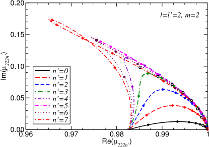
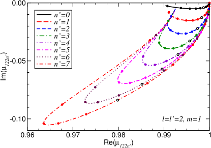
Figure 2: Trajectories traced by the mixing coefficients $\mu_{m\ell\ell^{\prime}n^{\prime}}$ with $\ell=\ell^{\prime}=2$, $m=2$ (left panel) and $m=1$ (right panel) as the Kerr parameter increases from $j=0$ (where $\mu_{m22n^{\prime}}=1$) to the nearly extremal Kerr limit. Each curve can be thought of as a parametric plot, where the parameter is $j$. Filled circles denote the following discrete values of $j$: $j=0,\,0.1,\,0.2,\,\dots,\,0.9,0.99$. To guide the eye, along each trajectory the dimensionless Kerr parameter $j=0.5$ is denoted by a hollow circle.

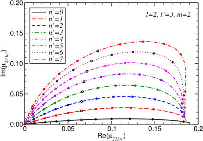
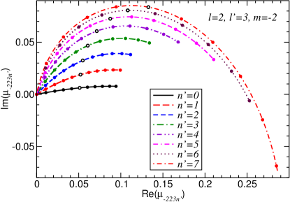
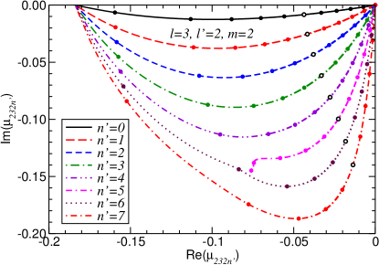
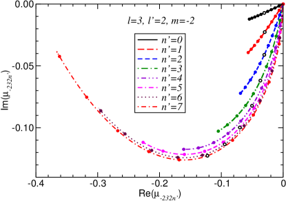
Figure 3: Trajectories traced by the mixing coefficients $\mu_{m\ell\ell^{\prime}n^{\prime}}$ in the complex plane as the Kerr parameter increases from $j=0$ (where $\mu_{m\ell\ell^{\prime}n^{\prime}}=0$ for $\ell\neq\ell^{\prime}$) to $j=1$. Panels in the top row refer to $(\ell,\,\ell^{\prime})=(2,\,3)$, those in the bottom row to $(\ell,\,\ell^{\prime})=(3,\,2)$; left panels are for $m=2$, right panels for $m=-2$.

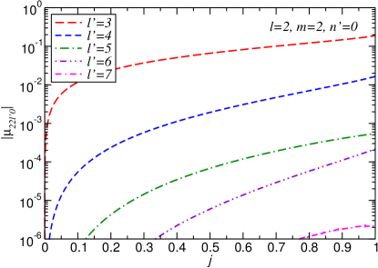
Figure 4: Absolute values of the mixing coefficients $|\mu_{m\ell\ell^{\prime}n^{\prime}}|$ with $\ell=m=2$, $n^{\prime}=0$ and different values of $\ell^{\prime}=3,\,\dots,7$, illustrating the roughly exponential decay of the mixing coefficients with $|\ell^{\prime}-\ell|$.

III Mixing coefficients

In this section we present and discuss our numerical results for both, the spherical-spheroidal mixing coefficients $\mu_{m\ell\ell^{\prime}n^{\prime}}(j)$ and the spheroidal-spheroidal mixing coefficients $\alpha_{m\ell\ell^{\prime}nn^{\prime}}(j)$. We also present power-law fits of the dependence of these coefficients on the dimensionless Kerr parameter $j$.

III.1 The spherical-spheroidal mixing coefficients

Fig. 2 shows how the mixing coefficients for $\ell=\ell^{\prime}=2$ and $m=2$ (left) or $m=1$ (right) behave for the first 8 QNMs ($n^{\prime}=0,\,\dots,\,7$) as the Kerr parameter increases from the Schwarzschild limit $j=0$ (where $\mu_{m\ell\ell^{\prime}n^{\prime}}=1$) to the extremal Kerr limit $j=1$. Each curve can be thought of as a parametric plot, where the parameter along the curve is $j$. Circles denote the following discrete values of $j$: $j=0,\,0.1,\,0.2,\,\dots,\,0.9,0.99$. The numerical data are truncated at $j=0.999$, because the behavior of QNMs for values of $j$ very close to unity requires a special treatment Yang et al. (2013a, b).

As first shown by Detweiler, for corotating modes with $\ell=m$ the imaginary part of the quasinormal frequencies goes to zero as $j\to 1$ Detweiler (1980). The physical reason for this behavior is that QNMs can be thought of as perturbations of null geodesics Mashhoon (1985); Cardoso et al. (2009); Yang et al. (2012, 2013a, 2013b). In the extremal limit the spherical photon orbit approaches the horizon and the frequency of most QNMs with $\ell=m$ becomes equal to $m\Omega_{\rm H}$, where $\Omega_{\rm H}=a/(2Mr_{+})$ is the angular velocity and $r_{+}=M+\sqrt{M^{2}-a^{2}}$ is the Boyer-Lindquist radius of the (outer) horizon. Whenever the QNM frequency tends to the critical value for superradiance $m\Omega_{\rm H}$ the black hole becomes marginally unstable, the eigenvalues of the SWSHs become real, and the SWSHs themselves become oblate in the language of Flammer’s monograph Flammer (1957). A surprising exception to this rule is the overtone with $n^{\prime}=5$: this oddity was first noticed by Onozawa (cf. Fig. 4 of Onozawa (1997)). As a consequence, the mixing coefficient corresponding to the mode with $n^{\prime}=5$ in the left panel of Fig. 2 is also exceptional, and it does not “turn around” to meet the other modes on the real axis as $j\to 1$.

Fig. 3 shows the dominant mixing coefficients for the first 8 QNMs ($n^{\prime}=0,\,\dots,\,7$) with $(\ell,\,\ell^{\prime})=(2,\,3)$, $(\ell,\,\ell^{\prime})=(3,\,2)$ and $m=2$ or $m=-2$. We choose to display these particular values of the mixing coefficients because they are the most relevant to explain the spherical-spheroidal mode mixing studied in Kelly and Baker (2013); London et al. (2014) (for the $m=2$ modes of comparable mass black-hole mergers) and Taracchini et al. (2014) (for the $m=\pm 2$ modes of extreme-mass-ratio black-hole mergers). Once again, note that the inner product becomes purely real near the superradiant frequency for modes with $m=2$, because the imaginary part of the QNM frequencies with $\ell=m$ tends to zero and the harmonics become oblate – the overtone with $n^{\prime}=5$ being, again, the exception. The plot also highlights the fact that the absolute value of the mixing coefficients is typically larger for large spins (at fixed overtone number $n^{\prime}$) and for large overtone numbers (at fixed spin $j$).

In Fig. 4 we plot the absolute value of the mixing coefficients $|\mu_{m\ell\ell^{\prime}n^{\prime}}|$ with $\ell=2$, $m=2$, $n^{\prime}=0$ as $\ell^{\prime}$ increases. The figure shows that (perhaps unsurprisingly) mode coupling decays roughly exponentially with $|\ell^{\prime}-\ell|$.

Numerical tables of $\mu_{m\ell\ell^{\prime}n^{\prime}}(j)$ for all modes with $|s|\leq\ell\leq 7$, $-\ell\leq m\leq\ell$, $-\ell^{\prime}\leq m\leq\ell^{\prime}$, $0\leq n^{\prime}\leq 7$ for $s=-2$, and $0\leq n^{\prime}\leq 3$ for $s=-1$ and $s=0$ can be found online rdw .

III.2 The spheroidal-spheroidal mixing coefficients

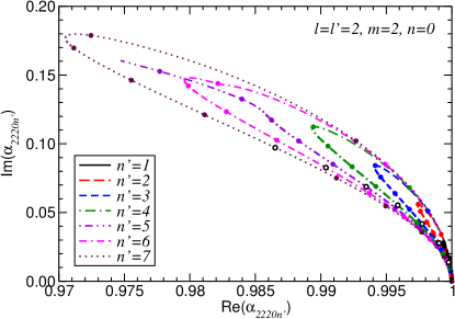
Figure 5: Trajectories described in the complex plane by the spheroidal-spheroidal mixing coefficients $\alpha_{m\ell\ell^{\prime}nn^{\prime}}(j)$ with $\ell=\ell^{\prime}=m=2$, $n=0$ and different values of the overtone index $n^{\prime}\geq 1$ as the dimensionless spin increases from $j=0$ to $j=1$.

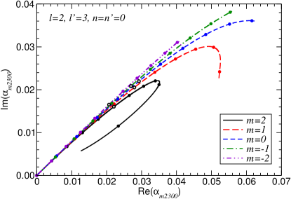
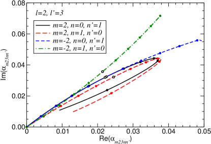
Figure 6: Trajectories described in the complex plane by the spheroidal-spheroidal mixing coefficients $\alpha_{m\ell\ell^{\prime}nn^{\prime}}(j)$ with: (1) $\ell=2$, $\ell^{\prime}=3$, $n=n^{\prime}=0$ and $-\ell\leq m\leq\ell$ (left panel); (2) $\ell=2$, $\ell^{\prime}=3$, $|m|=2$, and either $(n,\,n^{\prime})=(0,\,1)$ or $(n,\,n^{\prime})=(1,\,0)$.

Motivated by the fact that ringdown waveforms should be expanded in terms of SWSHs rather than spin-weighted spherical harmonics Berti et al. (2006a), Ref. Berti et al. (2006b) carried out a limited and preliminary investigation of the spheroidal-spheroidal mixing coefficients. Table I of Berti et al. (2006b) compared a numerical calculation of selected spheroidal-spheroidal mixing coefficients $\alpha_{m\ell\ell^{\prime}nn^{\prime}}(j)$, as defined in Eq. (6), with the Press-Teukolsky perturbation theory calculation. The constants $\alpha_{m\ell\ell^{\prime}nn^{\prime}}(j)$ computed using Leaver’s method were listed in Tables II and III of Berti et al. (2006b) for $j=0.8$ and selected values of the indices.

Here we extend those preliminary calculations to generic values of $j$ and to all modes of relevance for gravitational-wave data analysis. Representative results are shown in Figs. 5 and 6. Fig. 5 shows the scalar product between the dominant mode in black-hole binary merger simulations ($\ell=\ell^{\prime}=m=2$, $n=0$) and higher overtones with the same angular dependence (same $\ell=\ell^{\prime}=m$). All modes describe loops that begin and end close to $\alpha_{2220n^{\prime}}=1$; the one exception, as usual, is the QNM with $n^{\prime}=5$.

The most relevant spheroidal-spheroidal mixing coefficients to understand black-hole binary simulations are small-$n$ overtones with low angular indices $(\ell,~{}\ell^{\prime})$ equal to either $2$ or $3$. Some of these mixing coefficients are plotted, with the usual conventions, in Fig. 6. In particular, we show (1) the $m$-dependence of spheroidal-spheroidal overlaps when $\ell=2$, $\ell^{\prime}=3$, $n=n^{\prime}=0$, and (2) the overlap between the fundamental mode and the first overtone when $\ell=2$, $\ell^{\prime}=3$ and $|m|=2$.

III.3 Fitting formulas for the mixing coefficients

As illustrated in Fig. 1, we can reproduce the numerical data for the mixing coefficients to satisfactory accuracy (absolute deviations being typically smaller than $10^{-4}$ for the dominant modes, and smaller than a few times $10^{-3}$ for all modes we considered) with the following power-law fits:

$${\rm Re}(\mu_{m\ell\ell^{\prime}n^{\prime}}) = \delta_{\ell\ell^{\prime}}+p_{1}j^{p_{2}}+p_{3}j^{p_{4}}\,,$$

$${\rm Im}(\mu_{m\ell\ell^{\prime}n^{\prime}}) = q_{1}j^{q_{2}}+q_{3}j^{q_{4}}\,.$$ (11)

Table 1 lists the fitting parameters $(p_{i},\,q_{i})$ ($i=1,\dots\,,4$) for some combinations of $(m,\ell,\ell^{\prime},n^{\prime})$ that are particularly relevant in black-hole binary mergers. These values were chosen as particularly significant because

• Ref. London et al. (2014) successfully extracted QNMs with $(\ell,\,m,\,n)$=$(2,\,2,\,0)$, $(3,\,2,\,0)$ and $(2,\,2,\,1)$ from numerical simulations of comparable mass black-hole mergers, showing that mode mixing plays an important role in the extraction procedure; and

• Ref. Taracchini et al. (2014) pointed out that mode mixing plays an important role also for extreme mass-ratio binaries (see e.g. their Fig. 7). In addition, they found that negative-$m$, “counterrotating” modes (or “mirror modes”: see Berti et al. (2006a) for a discussion) contribute to the mixing, because frame dragging can change the sign of the orbital frequency of the plunging particle. This finding was confirmed by more recent time-domain calculations Harms et al. (2014).

Table 1 is only representative. Comprehensive tables listing these fitting parameters for scalar, electromagnetic and gravitational modes with $|s|\leq\ell\leq 7$, $-\ell\leq m\leq\ell$, $-\ell\leq m^{\prime}\leq\ell$, $0\leq n^{\prime}\leq 7$, $s=-2$ are publicly available online at rdw , where we also provide fitting parameters for the $\alpha_{m\ell\ell^{\prime}nn^{\prime}}$’s.

Indices				${\rm Re}(\mu_{m\ell\ell^{\prime}n^{\prime}})$				${\rm Im}(\mu_{m\ell\ell^{\prime}n^{\prime}})$
$m$	$\ell$	$\ell^{\prime}$	$n^{\prime}$	$10^{5}p_{1}$	$p_{2}$	$10^{5}p_{3}$	$p_{4}$	$10^{5}q_{1}$	$q_{2}$	$10^{5}q_{3}$	$q_{4}$
$2$	$2$	$2$	$0$	$-740$	$2.889$	$-661$	$17.129$	$1530$	$1.219$	$-934$	$24.992$
$2$	$2$	$2$	$1$	$-873$	$2.655$	$-539$	$15.665$	$4573$	$1.209$	$-2801$	$25.451$
$2$	$2$	$3$	$0$	$14095$	$1.112$	$4395$	$6.144$	$1323$	$0.854$	$-852$	$7.042$
$2$	$3$	$2$	$0$	$-10351$	$1.223$	$-5750$	$8.705$	$-1600$	$0.953$	$1003$	$14.755$
$-2$	$2$	$2$	$0$	$-1437$	$2.118$	$1035$	$2.229$	$-7015$	$1.005$	$67$	$3.527$
$-2$	$2$	$2$	$1$	$-2659$	$2.007$	$53$	$4.245$	$-21809$	$1.008$	$221$	$4.248$
$-2$	$2$	$3$	$0$	$14971$	$1.048$	$-5463$	$1.358$	$18467$	$1.015$	$-10753$	$1.876$
$-2$	$3$	$2$	$0$	$-13475$	$1.088$	$7963$	$1.279$	$-1744$	$1.011$	$516$	$1.821$

Table 1: Fitting function parameters in Eq. (11) for some of the $\mu_{m\ell\ell^{\prime}n^{\prime}}$’s that are most relevant in black-hole binary modeling.

IV Conclusions

This paper was mainly motivated by recent investigations of spherical-spheroidal mode mixing in black-hole binary mergers Buonanno et al. (2007); Kelly and Baker (2013); London et al. (2014); Taracchini et al. (2014). For this reason our analysis was limited to four-dimensional SWSHs and low-order overtones. Despite these limitations, we expect the “dictionary” developed in this paper to be useful in several applications of black hole perturbation theory, including the construction of phenomenological models of black-hole mergers, studies of Green’s functions in black-hole backgrounds, self-force investigations (see e.g. Casals et al. (2013); Wardell et al. (2014)) and calculations of Hawking radiation.

It would be interesting to extend our work to higher overtones, that may have some relation with black-hole area quantization (see e.g. Berti and Kokkotas (2003); Berti et al. (2003); Neitzke (2003); Berti et al. (2004); Hod and Keshet (2005); Keshet and Hod (2007); Keshet and Neitzke (2008); Kao and Tomino (2008)), or Berti (2004); Berti et al. (2009) for reviews). It would also be useful to investigate mixing coefficients for higher-dimensional spheroidal harmonics, that are of interest for the phenomenology of black-hole formation in high-energy particle collisions Kanti (2004) and to assess the stability of higher-dimensional rotating black holes Frolov and Stojkovic (2003); Ida et al. (2003); Berti et al. (2006b); Kunduri et al. (2006); Hoxha et al. (2000); Dias et al. (2012). Furthermore our analysis was limited to spin values that are not very close to $j=1$, and it calls for a more careful investigation of the nearly extremal regime, where a bifurcation of the spectrum can occur Yang et al. (2013a, b) and lead to turbulent behavior Yang et al. (2014).

The numerical data and fitting coefficients computed in this paper are publicly available for download rdw . The webpage includes also spherical-spheroidal mixing coefficients for SWSHs with $s=-1$ and $s=0$, that were not reported in this paper because they are qualitatively similar to the data for spin weight $s=-2$.

Appendix A Perturbative evaluation of the mixing coefficients

As mentioned in the main text, the SWSH equation can be solved via an expansion in powers of $c$ using standard perturbation theory Press and Teukolsky (1973). For $c=0$ the solutions are ordinary spin-weighted spherical harmonics Newman and Penrose (1966); Goldberg et al. (1967). The next-order correction can be found in Eq. (3.7) of Ref. Press and Teukolsky (1973) (see also Appendix F of Tagoshi et al. (1996)); the result is Eq. (4), where

$$\langle s\ell^{\prime}m|\mathfrak{h}_{1}|s\ell m\rangle=\int{}_{s}Y^{*}_{\ell^{\prime}m}\mathfrak{h}_{1}\,{}_{s}Y_{\ell m}\,d\Omega,\,$$ (12)

$$\mathfrak{h}_{1}\equiv(a\omega)^{2}\cos^{2}\theta-2a\omega s\cos\theta\,.$$ (13)

The integral can be evaluated using the identities

$$\langle s\ell^{\prime}m|\cos\theta|s\ell m\rangle$$

$$=\left(\frac{2\ell+1}{2\ell^{\prime}+1}\right)^{1/2}\langle\ell,1,m,0|\ell^{\prime},m\rangle\langle\ell,1,-s,0|\ell^{\prime},-s\rangle\,,$$

$$\langle s\ell^{\prime}m|\cos^{2}\theta|s\ell m\rangle=\frac{1}{3}\delta_{\ell,\ell^{\prime}}$$

$$+\frac{2}{3}\left(\frac{2\ell+1}{2\ell^{\prime}+1}\right)^{1/2}\langle\ell,2,m,0|\ell^{\prime},m\rangle\langle\ell,2,-s,0|\ell^{\prime},-s\rangle\,,$$

where $\langle\ell_{1},\ell_{2},m_{1},m_{2}|L,M\rangle$ is a Clebsch-Gordan coefficient.

References

- Thorne (1980) K. Thorne, Rev.Mod.Phys. 52, 299 (1980).
- Newman and Penrose (1966) E. Newman and R. Penrose, J.Math.Phys. 7, 863 (1966).
- Goldberg et al. (1967) J. Goldberg, A. MacFarlane, E. Newman, F. Rohrlich, and E. Sudarshan, J.Math.Phys. 8, 2155 (1967).
- Teukolsky (1973) S. A. Teukolsky, Astrophys.J. 185, 635 (1973).
- Press and Teukolsky (1973) W. H. Press and S. A. Teukolsky, Astrophys.J. 185, 649 (1973).
- Leaver (1986) E. W. Leaver, J. Math. Phys. 27, 1238 (1986).
- Leaver (1985) E. Leaver, Proc.Roy.Soc.Lond. A402, 285 (1985).
- Flammer (1957) C. Flammer, ed., Stanford University Press, Stanford, CA (1957).
- Kokkotas and Schmidt (1999) K. D. Kokkotas and B. G. Schmidt, Living Rev.Rel. 2, 2 (1999), arXiv:gr-qc/9909058 [gr-qc] .
- Berti et al. (2009) E. Berti, V. Cardoso, and A. O. Starinets, Class.Quant.Grav. 26, 163001 (2009), arXiv:0905.2975 [gr-qc] .
- Konoplya and Zhidenko (2011) R. Konoplya and A. Zhidenko, Rev.Mod.Phys. 83, 793 (2011), arXiv:1102.4014 [gr-qc] .
- Berti et al. (2006a) E. Berti, V. Cardoso, and C. M. Will, Phys.Rev. D73, 064030 (2006a), arXiv:gr-qc/0512160 [gr-qc] .
- Breuer (1977) R. A. Breuer, Gravitational Perturbation Theory and Synchrotron Radiation (Springer-Verlag, Lecture Notes in Physics 44, 1977).
- Fackerell and Crossman (1977) E. D. Fackerell and R. G. Crossman, Journal of Mathematical Physics 18 (1977).
- Seidel (1989) E. Seidel, Class.Quant.Grav. 6, 1057 (1989).
- Berti et al. (2006b) E. Berti, V. Cardoso, and M. Casals, Phys.Rev. D73, 024013 (2006b), arXiv:gr-qc/0511111 [gr-qc] .
- Onozawa (1997) H. Onozawa, Phys.Rev. D55, 3593 (1997), arXiv:gr-qc/9610048 [gr-qc] .
- Berti and Kokkotas (2003) E. Berti and K. D. Kokkotas, Phys.Rev. D68, 044027 (2003), arXiv:hep-th/0303029 [hep-th] .
- Berti et al. (2003) E. Berti, V. Cardoso, K. D. Kokkotas, and H. Onozawa, Phys.Rev. D68, 124018 (2003), arXiv:hep-th/0307013 [hep-th] .
- Neitzke (2003) A. Neitzke, (2003), arXiv:hep-th/0304080 .
- Berti et al. (2004) E. Berti, V. Cardoso, and S. Yoshida, Phys.Rev. D69, 124018 (2004), arXiv:gr-qc/0401052 [gr-qc] .
- Hod and Keshet (2005) S. Hod and U. Keshet, Class. Quant. Grav. 22, L71 (2005), arXiv:gr-qc/0505112 .
- Keshet and Hod (2007) U. Keshet and S. Hod, Phys. Rev. D76, 061501 (2007), arXiv:0705.1179 [gr-qc] .
- Keshet and Neitzke (2008) U. Keshet and A. Neitzke, Phys. Rev. D78, 044006 (2008), arXiv:0709.1532 [hep-th] .
- Kao and Tomino (2008) H.-c. Kao and D. Tomino, Phys. Rev. D77, 127503 (2008), arXiv:0801.4195 [gr-qc] .
- Buonanno et al. (2007) A. Buonanno, G. B. Cook, and F. Pretorius, Phys.Rev. D75, 124018 (2007), arXiv:gr-qc/0610122 [gr-qc] .
- Berti et al. (2007a) E. Berti, V. Cardoso, J. A. Gonzalez, U. Sperhake, M. Hannam, et al., Phys.Rev. D76, 064034 (2007a), arXiv:gr-qc/0703053 [GR-QC] .
- Schnittman et al. (2008) J. D. Schnittman, A. Buonanno, J. R. van Meter, J. G. Baker, W. D. Boggs, et al., Phys.Rev. D77, 044031 (2008), arXiv:0707.0301 [gr-qc] .
- Baker et al. (2008) J. G. Baker, W. D. Boggs, J. Centrella, B. J. Kelly, S. T. McWilliams, et al., Phys.Rev. D78, 044046 (2008), arXiv:0805.1428 [gr-qc] .
- Kelly et al. (2011) B. J. Kelly, J. G. Baker, W. D. Boggs, S. T. McWilliams, and J. Centrella, Phys.Rev. D84, 084009 (2011), arXiv:1107.1181 [gr-qc] .
- Pan et al. (2011) Y. Pan, A. Buonanno, M. Boyle, L. T. Buchman, L. E. Kidder, et al., Phys.Rev. D84, 124052 (2011), arXiv:1106.1021 [gr-qc] .
- Kelly and Baker (2013) B. J. Kelly and J. G. Baker, Phys.Rev. D87, 084004 (2013), arXiv:1212.5553 .
- London et al. (2014) L. London, J. Healy, and D. Shoemaker, (2014), arXiv:1404.3197 [gr-qc] .
- Taracchini et al. (2014) A. Taracchini, A. Buonanno, G. Khanna, and S. A. Hughes, (2014), arXiv:1404.1819 [gr-qc] .
- Harms et al. (2014) E. Harms, S. Bernuzzi, A. Nagar, and A. Zenginoglu, (2014), arXiv:1406.5983 [gr-qc] .
- Damour and Nagar (2014) T. Damour and A. Nagar, (2014), arXiv:1406.0401 [gr-qc] .
- Healy et al. (2014) J. Healy, P. Laguna, and D. Shoemaker, (2014), arXiv:1407.5989 [gr-qc] .
- Gualtieri et al. (2008) L. Gualtieri, E. Berti, V. Cardoso, and U. Sperhake, Phys.Rev. D78, 044024 (2008), arXiv:0805.1017 [gr-qc] .
- Campanelli et al. (2009) M. Campanelli, C. O. Lousto, H. Nakano, and Y. Zlochower, Phys.Rev. D79, 084010 (2009), arXiv:0808.0713 [gr-qc] .
- O’Shaughnessy et al. (2011) R. O’Shaughnessy, B. Vaishnav, J. Healy, Z. Meeks, and D. Shoemaker, Phys.Rev. D84, 124002 (2011), arXiv:1109.5224 [gr-qc] .
- Boyle et al. (2011) M. Boyle, R. Owen, and H. P. Pfeiffer, Phys.Rev. D84, 124011 (2011), arXiv:1110.2965 [gr-qc] .
- Boyle (2013) M. Boyle, Phys.Rev. D87, 104006 (2013), arXiv:1302.2919 [gr-qc] .
- Berti et al. (2007b) E. Berti, J. Cardoso, V. Cardoso, and M. Cavaglia, Phys.Rev. D76, 104044 (2007b), arXiv:0707.1202 [gr-qc] .
-
(44)
Webpage with Mathematica notebooks and
numerical quasinormal mode Tables:
http://www.phy.olemiss.edu/~berti/qnms.html . - Berti (2004) E. Berti, Conf.Proc. C0405132, 145 (2004), arXiv:gr-qc/0411025 [gr-qc] .
- Yang et al. (2013a) H. Yang, F. Zhang, A. Zimmerman, D. A. Nichols, E. Berti, et al., Phys.Rev. D87, 041502 (2013a), arXiv:1212.3271 [gr-qc] .
- Yang et al. (2013b) H. Yang, A. Zimmerman, A. Zenginoğlu, F. Zhang, E. Berti, et al., Phys.Rev. D88, 044047 (2013b), arXiv:1307.8086 [gr-qc] .
- Detweiler (1980) S. L. Detweiler, Astrophys.J. 239, 292 (1980).
- Mashhoon (1985) B. Mashhoon, Phys.Rev. D31, 290 (1985).
- Cardoso et al. (2009) V. Cardoso, A. S. Miranda, E. Berti, H. Witek, and V. T. Zanchin, Phys.Rev. D79, 064016 (2009), arXiv:0812.1806 [hep-th] .
- Yang et al. (2012) H. Yang, D. A. Nichols, F. Zhang, A. Zimmerman, Z. Zhang, et al., Phys.Rev. D86, 104006 (2012), arXiv:1207.4253 [gr-qc] .
- Casals et al. (2013) M. Casals, S. Dolan, A. C. Ottewill, and B. Wardell, Phys.Rev. D88, 044022 (2013), arXiv:1306.0884 [gr-qc] .
- Wardell et al. (2014) B. Wardell, C. R. Galley, A. Zenginoglu, M. Casals, S. R. Dolan, et al., Phys.Rev. D89, 084021 (2014), arXiv:1401.1506 [gr-qc] .
- Kanti (2004) P. Kanti, Int.J.Mod.Phys. A19, 4899 (2004), arXiv:hep-ph/0402168 [hep-ph] .
- Frolov and Stojkovic (2003) V. P. Frolov and D. Stojkovic, Phys.Rev. D67, 084004 (2003), arXiv:gr-qc/0211055 [gr-qc] .
- Ida et al. (2003) D. Ida, Y. Uchida, and Y. Morisawa, Phys.Rev. D67, 084019 (2003), arXiv:gr-qc/0212035 [gr-qc] .
- Kunduri et al. (2006) H. K. Kunduri, J. Lucietti, and H. S. Reall, Phys.Rev. D74, 084021 (2006), arXiv:hep-th/0606076 [hep-th] .
- Hoxha et al. (2000) P. Hoxha, R. Martinez-Acosta, and C. Pope, Class.Quant.Grav. 17, 4207 (2000), arXiv:hep-th/0005172 [hep-th] .
- Dias et al. (2012) O. J. Dias, G. T. Horowitz, D. Marolf, and J. E. Santos, Class.Quant.Grav. 29, 235019 (2012), arXiv:1208.5772 [gr-qc] .
- Yang et al. (2014) H. Yang, A. Zimmerman, and L. Lehner, (2014), arXiv:1402.4859 [gr-qc] .
- Tagoshi et al. (1996) H. Tagoshi, M. Shibata, T. Tanaka, and M. Sasaki, Phys.Rev. D54, 1439 (1996), arXiv:gr-qc/9603028 [gr-qc] .