Multi-frequency study of DEM~L299 in the Large Magellanic Cloud

Abstract

Aims. We have studied the H II region DEM L299 in the Large Magellanic Cloud (LMC) to understand its physical characteristics and morphology in different wavelengths.

Methods. We performed a spectral analysis of archived XMM-Newton EPIC data and studied the morphology of DEM L299 in X-ray, optical, and radio wavelengths. We used H$\alpha$, [S II], and [O III] data from the Magellanic Cloud Emission Line Survey (MCELS) and radio 21 cm line data from the Australia Telescope Compact Array (ATCA) and the Parkes telescope as well as radio continuum data (3 cm, 6 cm, 20 cm, 36 cm) from ATCA and from the Molonglo Synthesis Telescope (MOST).

Results. Our morphological studies imply that, in addition to the supernova remnant SNR B0543-68.9 reported in previous studies, a superbubble also overlaps the SNR in projection. The position of the SNR is clearly defined through the [S II]/H$\alpha$ flux ratio image. Moreover, the optical images show a shell-like structure that is located farther to the north and is filled with diffuse X-ray emission, which again indicates the superbubble. Radio 21 cm line data show a shell around both objects. Radio continuum data show diffuse emission at the position of DEM L299, which appears clearly distinguished from the H ii region LHA 120-N 164 that lies south-west of it. We determined the spectral index of SNR B0543-68.9 to be $\alpha=-0.34$, which indicates the dominance of thermal emission and therefore a rather mature remnant. We determined the basic properties of the diffuse X-ray emission for the SNR, the superbubble, and a possible blowout region of the bubble, as suggested by the optical and X-ray data. We obtained an age of $(8.9^{+9.2}_{-5.4})$ kyr for the SNR and a temperature of $(0.64^{+0.73}_{-0.20})$ keV for the hot gas inside the SNR, as well as a thermal energy content and temperature of the hot gas inside the superbubble of $(4.3^{+8.1}_{-2.6})\times 10^{50}\,\phi^{0.5}$ erg and $(0.74^{+0.36}_{-0.30})$ keV, with $\phi$ being the gas-filling factor.

Conclusions. We conclude that DEM L299 consists of a superposition of SNR B0543-68.9 and a superbubble, which we identified based on optical data.

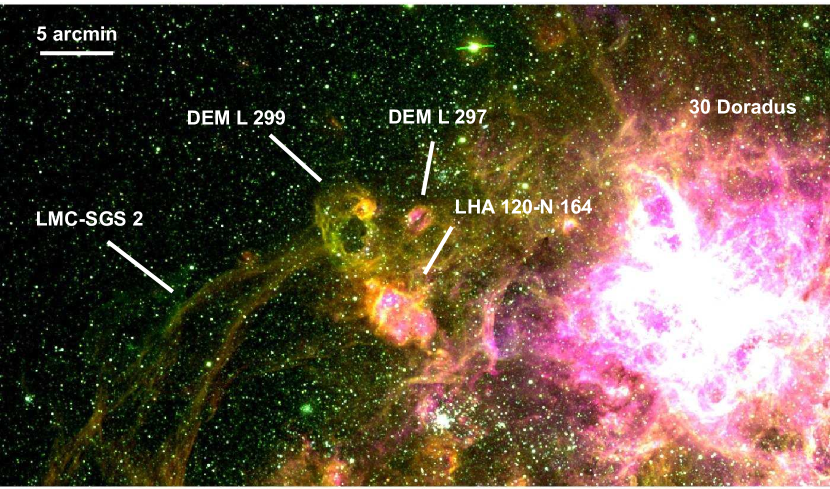
Figure 1: Regions around DEM L299 in the LMC with DEM L299 visible as a cavity, lying north-east of emission region LHA 120-N 164 and east of DEM~L297. Parts of the supergiant shell LMC-SGS 2 can be seen as filaments in the eastern part of the image, while 30 Doradus is visible as a bright emission region in the west. The image is created out of MCELS data and is a three-colour image showing the H$\alpha$ emission in red, [S II] emission in green, and [O III] emission in blue. The whole image shows an area of $60\arcmin\,\times\,34\arcmin$ ($\sim$ 870 $\rm pc\,\times\,500\leavevmode\nobreak\ \rm pc$). North is approximately in the upward direction, east is to the left.

1 Introduction

The interstellar medium (ISM) can be found mainly in three different phases (McKee & Ostriker 1977): a hot phase with temperatures of $\sim$ 10⁶ K, created through stellar winds and supernovae (SNe), observable in X-rays, for example, as supernova remnants (SNRs) or the interiors of bubbles, superbubbles, or supergiant shells; a warm phase with $\sim$ 10⁴ K, heated by the radiation of hot stars, for instance, observable as H II regions in optical emission lines; and a cold phase with temperatures $<$ 100 K, which is found for example in molecular clouds or H I regions, that are visible through the 21 cm hydrogen line. The ISM plays an important role for the understanding of the matter cycle, star formation, and stellar and galactic evolution.

DEM L299 is a complex H II region located in the Large Magellanic Cloud (LMC). It is found east of 30~Doradus and towards the northern rim of the supergiant shell LMC-SGS 2 and is therefore located close to active star-forming regions (see Fig. 1). The region was catalogued as an H$\alpha$ emission nebula (N 165) by Henize (1956) and harbours the supernova remnant SNR B0543-68.9. The remnant was classified as an SNR candidate (DEM L299) in the H$\alpha$ catalogue of Davies et al. (1976) and was optically confirmed to be an SNR by Mathewson et al. (1983). In X-rays, DEM L 299 has been observed and catalogued by the Einstein Observatory (Long et al. 1981; Wang et al. 1991) and ROSAT (Haberl & Pietsch 1999). The optical size of DEM L299 was determined by Desai et al. (2010) from optical data of the Magellanic Clouds Emission Line Survey (MCELS) to be $5\aas@@fstack{\prime}8\times 4\aas@@fstack{\prime}0$, which corresponds to $\sim$ $84\leavevmode\nobreak\ \rm pc\times 58\leavevmode\nobreak\ \rm pc$, assuming a distance to the LMC of 50 kpc (Pietrzyński et al. 2013), and has a central cavity of $1\aas@@fstack{\prime}8\times 2\aas@@fstack{\prime}3$ ($\sim$ $26\leavevmode\nobreak\ \rm pc\times 33\leavevmode\nobreak\ \rm pc$). With a diameter of 4$\aas@@fstack{\prime}$3 ($\sim$ $62\leavevmode\nobreak\ \rm pc$) the X-ray dimensions are about the same as in the optical, while the radio size of 3′ ($\sim$ 44 pc) is much smaller (Berkhuijsen 1986). At the north-western rim of DEM L299, there is a smaller H II region with a diameter of $\sim$ 1′ that is not associated with the SNR. This contains the young stellar object (YSO) and an OB-star (see Desai et al. 2010). In the south-west of DEM L299 lies the bright H II region LHA~120-N~164.

Since we found evidence that the H ii region DEM L299 also harbours a superbubble in addition to the supernova remnant SNR B0543-68.9, we use the nomenclature ’DEM L299’ only for the entire H ii region and not for the remnant, which has previously also been labelled ’DEM L299’.

The aim of this paper is to study this intriguing region using X-ray, optical, and radio observations to investigate the varied morphology of DEM L299 in the different energy bands. In Sect. 2 we describe the X-ray, optical, and radio data we used for our studies and the analysis of these data. The morphological studies can be found in Sect. 3, which contains comparative studies of X-ray, radio, and optical data. The X-ray spectral analysis of both objects is presented in Sect. 4, with a discussion of our results given in Sect. 5. In Sect. 6, we summarise our work and draw conclusions.

Table 1: Overview of the XMM-Newton X-ray observations of DEM L299 and the South Ecliptic Pole. The observations are background-flare filtered.

Observed Region	Obs.-ID	Obs.-Date	PI	Eff. Obs. Time for EPIC			Filter
				MOS1	MOS2	pn
				[ks]	[ks]	[ks]
DEM L299	0094410101	19.10.2001	Y.-H. Chu	11.2	11.3	7.9	Medium
South Ecliptic Pole	0162160101	24.11.2003	B. Altieri	11.9	12.3	8.6	Thin1
South Ecliptic Pole	0162160301	05.12.2003	B. Altieri	08.5	08.5	7.1	Thin1
South Ecliptic Pole	0162160501	14.12.2003	B. Altieri	09.4	09.2	7.0	Thin1

2 Data

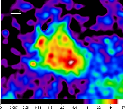
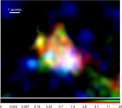
Figure 2: Left: intensity-scaled broadband XMM-Newton X-ray image of DEM L299. The image shows an area of $12\aas@@fstack{\prime}4\times 10\arcmin\$ in the energy range of 0.3–8.0 keV and has been smoothed by a Gaussian with a kernel radius of four pixels, after being adaptively smoothed. Right: three-colour image created out of XMM-Newton data. Red: 0.3–0.8 keV, green: 0.8–1.5 keV, blue: 1.5–4.5 keV. To create the image, the same area, the same kernel radius, and the same scale units were used as for the broadband image. The scales are in counts/s/deg².

2.1 X-ray data

For the X-ray studies, we analysed the archived data of the European Photon Imaging Camera (EPIC) of the ESA satellite XMM-Newton (Jansen et al. 2001) with Obs.-ID 0094410101 (PI: Y.-H. Chu) from the year 2001. The observation was performed in full-frame mode and has an effective observation time of $\sim$ 11 ks for the EPIC MOS1 and EPIC MOS2 detectors (Turner et al. 2001), and $\sim$ 8 ks for the EPIC pn detector (Strüder et al. 2001). Table 1 summarises the observations.

We processed the data with the XMM-Newton Extended Source Analysis Software (XMM-ESAS) package version 4.3 (Snowden & Kuntz 2011a, b), which is part of the XMM-Newton Scientific Analysis Software version 11.0.0 (SAS). We filtered out soft proton flares by light-curve screening, removed point sources, subtracted the quiescent-particle background using filter-wheel-closed data and unexposed corners of the detectors, and checked for EPIC MOS CCDs operating in an anomalous state. This is a state that shows an enhanced background in the energy range $\la 1$ keV (Kuntz & Snowden 2008). MOS1 CCD#5 was identified to be in this state and was therefore excluded from our analysis. More details about these ESAS procedures can be found in Snowden et al. (2008).

To estimate the cosmic X-ray background (CXB) for the spectral analysis, we used three archived XMM-Newton EPIC observations of the South Ecliptic Pole (SEP) from 2003 with Obs.-IDs 0162160101, 0162160301, and 0162160501 (PI: B. Altieri). We assumed that the CXB of the SEP observations is representative of the DEM L299 observation. All three SEP observations have been taken in full-frame mode and result in a total effective observation time of $\sim$ 30 ks (see Table 1). The data of these observations were analysed in the same way as described above. For Obs.-ID 0162160301, MOS1 CCD#4 was found to be operating in an anomalous state and thus excluded from further analysis. The resulting data sets of these three observations were combined to obtain one dataset with an effective exposure time of 30 ks for the MOS1 and MOS2 detectors, and 23 ks for the pn detector.

Images of DEM L299 created out of the XMM-Newton data are shown in Fig. 2 (see Sect. 3 for details).

2.2 Optical data

For our optical studies, we used H$\alpha$, [S II], and [O III] data of the MCELS (e.g. Smith et al. 2000), which mapped the Large and the Small Magellanic Clouds in H$\alpha$ (6563 Å), [S II] (6724 Å), [O III] (5007 Å), and at two continuum bands, which were used to subtract the stellar continuum emission. The survey was carried out by the University of Michigan (UM) and the Cerro Tololo Inter-American Observatory (CTIO) and was performed with the UM/CTIO Curtis Schmidt telescope situated in Chile. This telescope is a 0.6 m Schmidt telescope with a resolution of 2$\aas@@fstack{\prime\prime}$3/pixel. Its camera is a SITE $2048\times 2048$ CCD and produces images with a field of view of $1.35^{\circ}\times 1.35^{\circ}$ per image. The data we used for our studies were sky-subtracted, flux-calibrated, and continuum-subtracted. For the smoothed images created out of these data, the exposure time was normalised to one second.

2.3 Radio-continuum data

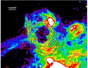
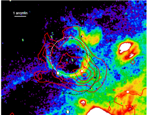
Figure 3: MCELS images in H$\alpha$ (left) and [O III] (right). The images are continuum-subtracted, flux-calibrated, sky-subtracted, and smoothed. The same area of the sky is shown as in the X-ray images in Fig. 2. The contours are taken from the smoothed X-ray broadband image, with 5 contour levels at 18, 28.5, 39, 49.5, and 60 counts/s/deg². The white dashed circle shows the position of the H$\alpha$ cavity, and the black dashed circle the position of the shell in the [S II]/H$\alpha$ image (see Fig. 4).

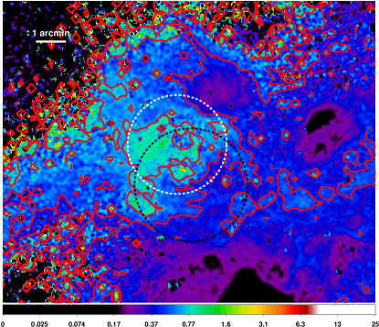
Figure 4: [S II]/H$\alpha$ flux-ratio image created out of the flux-calibrated, continuum-subtracted MCELS H$\alpha$ and [S II] data (see Fig. 3). A circular structure is visible, indicated by the black dashed circle. The north-eastern part of this structure has a [S II]/H$\alpha$ flux ratio greater than 0.67 and thus seems to be shock-ionised. Therefore, this structure is indicative of an SNR. The position of the H$\alpha$ cavity is marked in white. The flux ratio contours are shown with contour levels at 0.46 and 0.67. The area of the sky is the same as in Fig. 3.

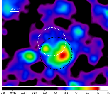
Figure 5: Intensity-scaled X-ray image of DEM L299 in an energy range of 1.5–4.5 keV. The black dashed circle indicates the position and size of the SNR as indicated through the [S II]/H$\alpha$ flux ratio image (Fig. 4), and the white dashed circle the superbubble as indicated through the optical images (Fig. 3). Most of the hard X-ray emission is confined inside the SNR region. Area of the sky, scale units, and smoothing parameters are the same as in Fig. 2.

We used radio observations at four frequencies (see Table 2) to study and measure flux densities of DEM L299. For the 36 cm (Molonglo Synthesis Telescope, MOST) flux density measurement given in Table 2 we used unpublished images as described by Mills et al. (1984), and for the 20 cm we used image from Hughes et al. (2007). The Australia Telescope Compact Array (ATCA) project C634 (at 6/3 cm) observations were combined with mosaic observations from project C918 (Dickel et al. 2005). Data for project C634 were taken by the ATCA on 1997 October 6/7 and 17/18, using the array configuration EW375 and 750C. For the final image (Stokes parameter I) we excluded baselines created with the $6^{\mathrm{th}}$ ATCA antenna, leaving the remaining five antennas to be arranged in a compact configuration. C634 observations were carried out in snap-shot mode, totalling $\sim$ 4.5 hours of integration over two 12 hour periods. Source PKS B1934–638 was used as the primary calibrator and source PKS B0530–727 as the secondary calibrator. The miriad (Sault & Killeen 2006) and karma (Gooch 1996) software packages were used for reduction and analysis. The 6 cm and 3 cm images were constructed using miriad multi-frequency synthesis (Sault & Wieringa 1994). Deconvolution was achieved with the clean and restor tasks with primary-beam correction applied using the linmos task. Similar procedures were used for the U and Q Stokes parameters. Using the flux density measurements shown in Table 2, we estimated a radio spectral index for DEM L299 of $\alpha=-0.34\pm 0.03$. More information on the observing procedure and other sources observed in this session/project can be found in Bojičić et al. (2007), Crawford et al. (2008a, b, 2010), Cajko et al. (2009), de Horta et al. (2012), Grondin et al. (2012), Haberl et al. (2012), Maggi et al. (2012), Kavanagh et al. (2013), and Bozzetto et al. (2010, 2012a, 2012b, 2012c, 2012d, 2013).

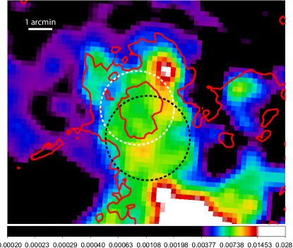
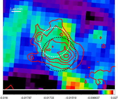
Figure 6: Left: 20 cm radio-continuum image of DEM L299 with overlaid H$\alpha$ contours, showing the same area of $12\aas@@fstack{\prime}4\times 10\arcmin\$ as the X-ray images in Fig. 2. The image was smoothed with a Gaussian using a kernel radius of one pixel. The contours are taken from the H$\alpha$ image in Fig. 3 with one contour level at 2. The black dashed circle indicates the position of the SNR, while the white dashed circle shows the position of the superbubble. The scales are in Jy/beam. Right: same as left, but for the 36 cm radio-continuum data and with the same X-ray contours as in Fig. 3.

3 Morphology studies

3.1 X-rays

To create smoothed, exposure-corrected images in different energy bands, we combined the data of the MOS1, MOS2, and pn detectors using ESAS, rebinned the data with a factor of two, and adaptively smoothed it with a smoothing counts value of 50 using the ESAS task adapt_900. Afterwards, the images were smoothed again with a Gaussian using a smoothing kernel radius of four pixels for a better presentation.

A zoom-in on the DEM L299 region is shown on the left side of Fig. 2 in the energy range of 0.3–8.0 keV (broadband). We furthermore created images in energy bands of 0.3–0.8 keV (soft band), 0.8–1.5 keV (medium band), and 1.5–4.5 keV (hard band). These images were combined to produce the three-colour image on the right side of Fig. 2. Both images show the same area of the sky with a size of $12\aas@@fstack{\prime}4\times 10\arcmin$, which corresponds to $\sim$ 180 $\rm pc\times 145\leavevmode\nobreak\ \rm pc$. At the northern rim of DEM L299, a point-source was excluded that correlates with the position of the stellar X-ray source [SHP2000] LMC 347 (Sasaki et al. 2000). The highest X-ray emission is reached in the south-west (see Fig. 2, left). This part is bright in all three energy bands, as can be seen in the three-colour image on the right side of Fig. 2, where it appears white in colour. Since the emission around the brightest region declines in all three energy bands and not only in the soft energy band, the difference in brightness does not seem to be an effect of absorption.

3.2 Optical

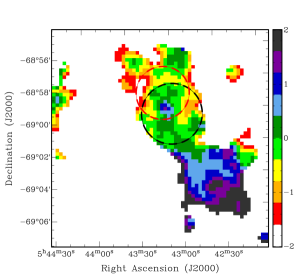
Figure 7: Spectral index map of the DEM L299 region created out of the 20 cm and 36 cm images. The position of the SNR and of the superbubble are marked in black and red (white in other figures). DEM L299 can be easily distinguished from the H II region LHA 120-N 164, which lies to the south-west of it, because of their different spectral indices.

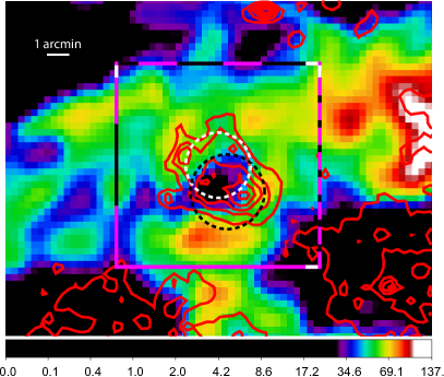
Figure 8: Combined ATCA and Parkes H I 21 cm radio data showing a velocity slice at $\sim$ 264 km/s in the region of $22\arcmin\ \times 17\arcmin\$ around DEM L299 with overlaid X-ray contours of Fig. 2. Scales represent the brightness temperature and are in Kelvin. The data have been smoothed by a Gaussian using a kernel radius of two pixels. The black dashed circle indicates the approximate size and position of the SNR based on the [S II]/H$\alpha$ ratio, while the white dashed circle marks the position of the H$\alpha$ cavity. The box indicates the area that we used to create the images in Fig. 9 at different heliocentric velocities and the position-velocity images shown in Fig. 10. The different line styles of the box mark its individual sides and their orientation (white mark), for an easier comparison with the plots shown in Fig. 10.

We created sky-subtracted, flux-calibrated, continuum-subtracted, and smoothed images from the MCELS data. These images can be seen in Fig. 3 and show the same area of the sky as in Fig. 2 in H$\alpha$ (left side) and [O III] (right side), with overlaid X-ray contours.

These images reveal a completely different appearance of DEM L299 in the optical than in X-rays. The emission line images are dominated by a circular shell-like structure, which is about 4′ ($\sim$ 60 pc) in diameter and possess a visible cavity with a diameter of $\sim$ 2$\aas@@fstack{\prime}$5 ($\sim$ 35 pc). Compared with the X-ray image, the optical cavity lies in the eastern, fainter part of the X-ray emission, and does not include the brightest area of X-ray emission in the south-west. The border of the supergiant shell LMC-SGS 2 can be seen as a filament east of DEM L299. While the optical shell is quite clearly defined in the west and the east (cf. [O iii], Fig. 3, right side), the north-north-eastern border shows less emission and is much more diffuse than the rest of the shell-like structure. The [S II] emission (not shown here) bears a strong resemblance to the H$\alpha$ emission (Fig. 3, left). The [O iii] emission (Fig. 3, right) shows some distinct differences than the H$\alpha$ and [S II] emission. The shell of the cavity is much narrower with a very circular shape. There is a break in this shell in the north-east where the H$\alpha$ and [S II] emission show a diffuse structure (see Fig. 3), indicating a possible blowout. This suggestion is supported by a slight enhancement of the X-ray emission in this region, which is discussed in Sect. 4. The main difference between these optical images is the lack of [O iii] emission in the south-west below the cavity, which is located just south of the brightest region in X-rays.

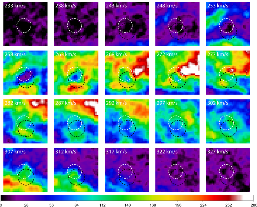
Figure 9: H I data cube channel maps showing the H I distribution for a certain heliocentric velocity interval. Each plot is created out of three velocity slices, corresponding to a velocity interval of $\sim$ 5 km/s from top left to bottom right. The upper left plot starts with a mean heliocentric velocity of $\sim$ 233 km/s, the last plot in the lower right with $\sim$ 327 km/s. The black dashed circle marks the position of the SNR, while the white dashed circle corresponds to the H$\alpha$ cavity. Each image shows an area of $10\aas@@fstack{\prime}3\times 10\aas@@fstack{\prime}3$, which is also indicated by the box in Fig. 8. Scales represent the brightness temperature and are in Kelvin.

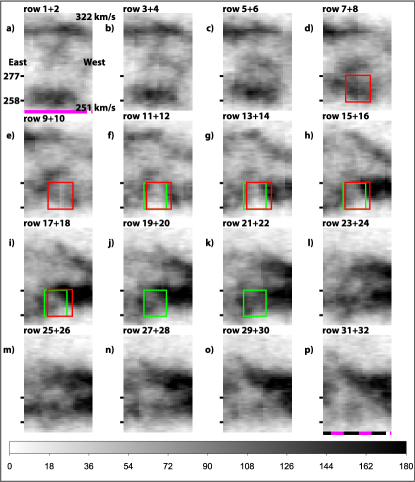
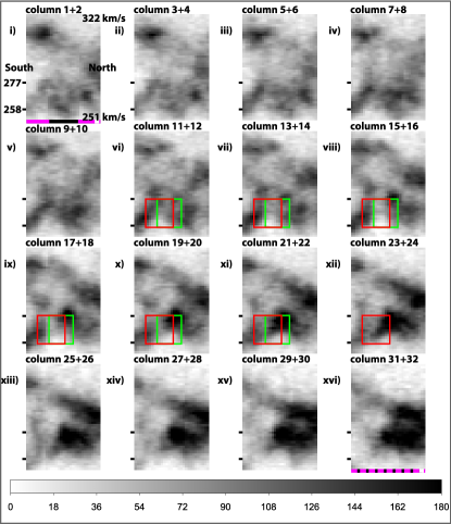
Figure 10: Average H i distribution image of the DEM L299 region at a certain position (left: east-west direction, right: south-north direction) for a velocity range of 251–322 km/s. Left: position-velocity plot showing the intensity of the H i emission in dependence of the velocity (ordinate) of the gas within the box in Fig. 8 against its position (abscissa) in the east-west direction of that box. The ordinate shows the velocity in the range of 251 km/s (at the bottom of each plot) to 322 km/s (at the top of each plot), with a velocity resolution of 1.649 km/s. The abscissa covers a range of 10$\aas@@fstack{\prime}$3 in east-west direction, corresponding to $\sim$ 150 pc at the LMC distance. The different plots show from a) to p) the velocity information for two added pixel rows of the box in Fig. 8, as indicated above each plot. These pixel rows are taken from the box of Fig. 8 from bottom to top. Since the abscissa of plot a) corresponds to the lowest two pixel rows of the box in Fig. 8, both are marked with a magenta line of the same line style (here: solid), also indicating their orientation through a white bar, for an easier comparison of these plots with Fig. 8. The same holds for plot p). The red rectangle indicates the position of the SNR as indicated by the [S II]/H$\alpha$ flux ratio, while the green rectangle shows the position of the H$\alpha$ central cavity. The velocity range of these rectangles corresponds to 258–277 km/s, as determined for the SNR and the superbubble in Fig. 9. This velocity range is marked in the plots by two black tick marks. Scales are in Kelvin. Right: same as left, but for the south-north direction of the box in Fig. 8, i.e. for the different pixel columns of the box (stepped from left to right) instead of pixel rows.

To determine the exact position of the SNR, we examined the flux ratio of [S II] and H$\alpha$. Fesen et al. (1985, and references therein) stated that a [S II]/H$\alpha$ flux ratio of $\gtrsim$ 0.67 is a strong indication for the shock-ionised shell of an SNR that is located in an H II region. We created a [S II]/H$\alpha$ ratio image as shown in Fig. 4. In this image, a clear circular structure with an enhanced [S II]/H$\alpha$ ratio is visible (black dashed circle). This circular structure has its centre at RA 05:43:02.2, Dec -69:00:00.0 (J2000) and a radius of $\sim$ 2′ ($\sim$ 30 pc). Emission located along the north-eastern rim of this structure shows a flux ratio of $\geq 0.67$, which is an indicator for shock-ionised gas. Most likely, this structure represents the border of the SNR. Surprisingly, this shell is not at the same position as the H$\alpha$ cavity (cf. Fig. 4, left side). Its centre lies $\sim$ 1$\aas@@fstack{\prime}$4 more to the south and $\sim$ 0.5′ more to the west than the centre of the cavity. In contrast, no shell-like structure is visible in the [S II]/H$\alpha$ image at the position of the cavity in H$\alpha$ or [O III]. This led us to conclude that we see a superposition of two separate objects: an SNR and a superbubble. The superbubble lies north of the SNR and corresponds to the position of a shell clearly visible in [O III], with some overlap. The south-western part of the SNR, which has a lower flux ratio, corresponds to the position of the X-ray bright region, which is confined inside the borders of the optical SNR (see Fig. 5).

3.3 Radio-continuum

The 20 cm and 36 cm radio-continuum data of the DEM L299 region are shown in Fig. 6. The two images show the same area of the sky as the X-ray images in Fig. 2. The 20 cm and 36 cm images show extended emission coincident with the X-ray position of DEM L299. The emission follows the H$\alpha$ emission rather than the X-ray emission (see Fig. 6, left). A shell-like structure can be seen in the 36 cm image, corresponding to the position of the two objects. Figure 7 shows the spectral index map of DEM L299 using the 36 cm and 20 cm images. This spectral index map allows a clear differentiation of the SNR from the H II region LHA 120-N 164, which lies south-west of it (see Fig.1). However, our spectral index estimate for the entire SNR ($\alpha=-0.34$) based on all measured flux densities is slightly on the flatter side, indicating the dominance of the thermal emission and the therefore somewhat older age of the remnant. We also point out that the H II region LHA 120-N 164 shows the canonical values of $\alpha\approx\,$+0.4.

Table 2: Integrated flux densities of DEM L299. The flux density was estimated using images from Mills et al. (1984) at $\lambda$=36 cm and from Hughes et al. (2007) at $\lambda$=20 cm.

$\nu$	$\lambda$	Beam Size	R.M.S	STotal
(MHz)	(cm)	(″)	(mJy)	(mJy)
0843	36	43.0$\times$43.0	0.50	154
1377	20	40.0$\times$40.0	0.50	146
4800	06	17.3$\times$14.0	0.11	91
8640	03	17.3$\times$14.0	0.06	72

3.4 H I 21 cm

To investigate the relative position of the SNR and the superbubble, we investigated the 21 cm emission line map of neutral hydrogen. We downloaded combined ATCA and Parkes H I 21 cm radio data in the direction of DEM L299 from the Magellanic Cloud Survey web page. More information about the survey can be found in Kim et al. (1998, 2003). Figure 8 shows the neutral hydrogen in an area of $22\arcmin\times 17\arcmin$ ($\sim$ 320 $\rm pc\times 247\leavevmode\nobreak\ \rm pc$) with a heliocentric velocity of $\sim$ 264 km/s, which we chose since it shows a clear shell-like structure. As can be seen in Fig. 8, the position of the SNR and the possible superbubble coincide with an area of low H I emission. Around them, a shell-like structure with stronger H I emission is visible that surrounds both objects. This shell can also be seen in Fig. 9, which shows the H I data for different velocity slices between 233–327 km/s. The shell is visible at velocities from 258–277 km/s (images in the second row). This suggests the existence of a hydrogen shell that surrounds both objects, indicating that both objects are close to each other.

The H I catalogue in Kim et al. (2007) assigns a velocity of 276.24 km/s ($\sigma$ = 7.798 km/s) to the large H I cloud projected towards DEM L299, and Points et al. (1999) determined the heliocentric velocities of the front- and backside of SGS-LMC 2 to be $\sim$ 250 km/s and $\sim$ 300 km/s, as can be seen in Fig. 9, e.g., at 302 km/s to 312 km/s, with DEM L299 being projected along the northern rim of this supergiant shell.

Out of the Magellanic Cloud Survey H i data, we created a H i map at a certain position corresponding to a narrow line in the projected sky over a range of velocities, which we call position-velocity plots. These plots are presented in Fig. 10 and show the intensity of the H i emission as a function of the velocity of the gas within the box of Fig. 8 plotted against its RA and its Dec position (left and right side of Fig. 10). For every position-velocity plot, we combined two pixel rows (or columns) of Fig. 8. According to the resolution of the Magellanic Cloud Survey, the velocity information has a resolution of 1.649 km/s. We chose the velocity extensions of the boxes that indicate the position of the SNR and of the superbubble based upon the existence of a radio shell at the respective velocity slice of Fig. 9. In these position-velocity plots, an enhanced emission can be recognized at velocities that Points et al. (1999) determined for the borders of SGS-LMC 2, visible as horizontal lines in the plots of Fig. 10a)–d). Furthermore, a circular structure of enhanced emission is visible in the plots of Fig. 10ix)–xv), which corresponds to the projected Dec position of the YSO 2MASS J05425375-6857116 that lies north-west of DEM L299 with respect to the position of the SNR and the superbubble. This feature is centred at a velocity of $\sim\,275$ km/s and has an extent of $\pm$8 km/s.

At the position of the SNR and the superbubble, the position-velocity plots show an enhanced 21 cm line emission feature at the position where a common shell of neutral hydrogen around both objects would be expected to lie within projection. Although there is evidence for a hydrogen shell, the data do not allow us to distinguish between a common shell around both objects or two separate shells. Since in particular the border of the shell that lies at lower velocities cannot be clearly distinguished, the data are ambiguous and require further studies, which goes beyond the scope of this paper.

4 Spectral analysis

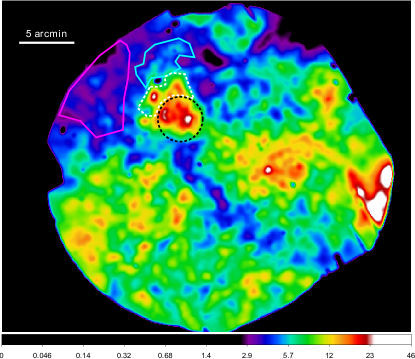
Figure 11: FOV of the XMM-Newton observation 0094410101 in an energy band of 0.8–1.5 keV, smoothed by a Gaussian with a kernel radius of three pixels. The colour-scale is in units of counts/s/deg². The marked areas are the fitting regions used for the spectral fits of the SNR (black), the part of the superbubble that does not overlap the SNR (white), the blowout of the superbubble (cyan), and the local background (magenta).

We analysed the XMM-Newton EPIC spectra to investigate the properties of the hot gas of DEM L299. The fitting was performed with Xspec version 12.7.1 (Arnaud 1996). The model we used for the background is based upon the example given in the ESAS cookbook (see footnote 1). To estimate the X-ray background, our model includes an unabsorbed thermal component (Xspec-model: apec) for the Local Hot Bubble with $k_{\mathrm{B}}T=0.1$ keV, two thermal components that are absorbed by the Milky Way (Xspec-models: phabs $\times$ (apec + apec)) for the cooler halo emission with $k_{\mathrm{B}}T=0.1$ keV and the hotter halo with $k_{\mathrm{B}}T=0.5$ keV. The unresolved extragalactic background was modelled using an absorbed power law (Xspec-model: powerlaw) with a spectral index $\alpha=1.46$ (Chen et al. 1997), which is absorbed by the Milky Way (Xspec-model: phabs) and the LMC (Xspec-model: vphabs) ISM. For the Milky Way, an $N_{\rm H,MW}$ of $0.06\times 10^{22}$ cm^-2 was assumed (Dickey & Lockman 1990). The chemical abundances for the LMC were set to $50$ % of solar abundances (Russell & Dopita 1992). This X-ray background was estimated by simultaneously fitting the used LMC observation and the three combined SEP observations, with frozen energies, photon index, and $N_{\rm H,MW}$, and with linked normalisations between all detectors and observations.

To account for instrumental fluorescence lines, Gaussians with zero width are included in the model, e.g. for MOS1 and MOS2 at $1.49$ keV ($\@element{\mathrm{Al}}$ K$\alpha$) and $1.75$ keV ($\@element{\mathrm{Si}}$ K$\alpha$), and for pn at $1.49$ keV ($\@element{\mathrm{Al}}$ K$\alpha$). The more energetic fluorescence lines were also fitted, but since the emission above $\sim$ 4 keV is irrelevant for these soft X-ray studies, they are not listed here. The energies were fitted and then frozen, while their normalisations remained free for every detector and observation. Another Gaussian was added at $0.65$ keV to account for possible O VIII emission caused by solar wind charge exchange (SWCX) as reported in Koutroumpa et al. (2009) for all three SEP observations.

The residual soft proton spectrum was fitted in a separate power-law model for each detector and each observation. The power laws are not folded with the instrumental response matrix, but instead through a diagonal unitary response matrix. While their normalisations were fitted freely, the statistics of the data were not high enough to do the same for the photon index. Hence, the photon index of each power law was set to one, lying within the reasonable range between 0.2–1.3 (see ESAS cookbook v4.3).

To model the background that was determined by the SEP data, the SEP spectrum was multiplied by a factor to correct for the different areas. As a test for the appropriateness of our background estimation through the SEP observations, we extracted the spectrum of a region as local background within the same pointing as the superbubble and SNR. This local background region is marked in magenta in Fig. 11 and lies east of the superbubble and SNR in a region of the FOV as empty as possible. We fitted the spectra of this region simultaneously with the combined SEP observations to detect deviations. The local background spectrum has a slight excess, indicating that an additional thermal component is necessary, probably as a result of local hot ISM in the busy FOV. The fitting results are listed in Table 3. However, the statistics of this region are far too low to take this area for background estimation instead of the SEP observations, but we consider its contribution in the following discussion.

Since the projections of the SNR and the superbubble strongly overlap (cf. Fig. 5), there should be an additional emission component of the superbubble in the spectrum of the SNR and vice versa. To take this into account, we defined a polygonal region for the fits of the superbubble that does not overlap the remnant as defined by the [S II]/H$\alpha$ data, so that no additional emission component accounting for the SNR emission is needed in the model for this polygonal superbubble-only region. We first fitted this superbubble-only spectrum. Since the SNR has well-defined borders through the circular structure in the [S II]/H$\alpha$ image, we took this circle as our extraction region for the SNR (see Fig. 11 for the fitting regions). To investigate a possible blowout of the superbubble to the north-east, as strongly indicated by the optical and X-ray data, we performed a spectral analysis of this blowout region as marked in cyan in Fig. 11, which shows the whole FOV of the XMM-Newton observation in an energy range of 0.8–1.5 keV.

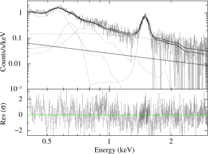
Figure 12: Fitted pn spectrum of the SEP observation used for estimating the local X-ray background in an energy range of 0.4–3.0 keV with model components and residuals. This spectrum has been fitted simultaneously with the SNR spectrum shown in Fig. 13. The straight line is the modelled residual soft proton component. Crosses are data points, while the solid line shows the fitted model. The model components are dotted.

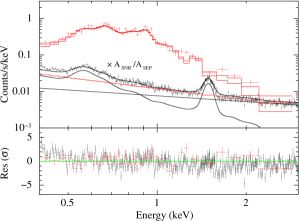
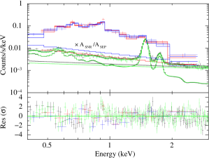
Figure 13: Fitted source and background spectra for the SNR for pn (left) and MOS1/2 (right) with residuals in the energy range of 0.4–3.0 keV. The component for the SNR emission was fitted with a vpshock model. The straight lines are the modelled residual soft proton components for the corresponding detector and observation. Crosses stand for data points, while the solid lines are the fitted models. The source spectra are plotted in red (pn and MOS1) or blue (MOS2) and the the background spectra in black (pn and MOS1) or green (MOS2). For better presentation, the background spectra are scaled down to the area of the SNR region, which was much smaller than the extraction region for the SEP spectrum.

For the spectra, the data were binned to a minimum of 50 counts per channel and were fitted in an energy range of 0.3–10.0 keV. We first fitted the combined SEP observations simultaneously with the individual DEM L299 regions to estimate the X-ray photon background. For the source component, we first tried the apec model (Smith et al. 2001), which is a thermal plasma model with a bremsstrahlung continuum and line emission. However, no good fits were achieved. We then tried two different non-equilibrium models: a non-equilibrium ionisation plasma model (Xspec model: vnei, Borkowski (2000)), and a plane-parallel shocked plasma model (Xspec model: vpshock, Borkowski (2000)). For the parameters of these two components, we fixed the metal abundances at 50 % of the solar abundances, appropriate for the LMC.

To fit the SNR spectrum, we added an additional thermal emission component to our model to account for the superbubble emission in this region. We froze the temperature and ionisation timescale $\tau$ of this superbubble component to the fitted values we derived from our fits of the polygonal superbubble-only region. The normalisation was frozen as well after multiplying it with a factor to account for the different sizes of the polygon and the approximate overlap region of the superbubble with the SNR fitting region.

Since the large number of included model components bear an uncertainty, we performed a series of fits in which we tested more than 20 different temperatures in the range between 0.1 keV and 7 keV for both the superbubble and the remnant. This resulted in several favoured sets of fitting results, which we compared based on the goodness of the fit and the ability to determine the 90 % uncertainty limits for the parameters. Compared with these two regions, the SEP data have a much higher count statistic and therefore dominate the goodness of the fit (cf. Figs.12, 13). To obtain a more meaningful fit of the superbubble and remnant spectra, we first fitted the entire data as described before, then froze all background components at these fitted values, removed the SEP data, and just fitted the DEM L299 spectra with the previously estimated and frozen background components. With this method, we now obtained more meaningful reduced chi-squared for the different sets of fitting results.

Table 3: Resulting best-fit parameters for the polygon (i.e. part of the superbubble), SNR, superbubble blowout, and local background region. For all regions, the best-fit values were obtained with the vpshock model. The column density $n_{\mathrm{H,LMC}}$ is given in units of $10^{22}$ cm^-2, the temperature $k_{\mathrm{B}}T_{\mathrm{x}}$ in keV, the ionisation timescale $\tau$ in s cm^-3, and the normalization $norm$ in cm^-5. The parameter $norm$ is the normalisation of the Xspec model vpshock and is a function of the emission measure. In the last row, the reduced $\chi^{2}$ of the fit is given. The uncertainties given are the upper and lower 90 % confidence ranges.

	Polygon	SNR	Blowout	Local Bkg
$nH_{\mathrm{LMC}}$	0.30 (0.07–0.66)	0.66 (0.59–0.77)	0.27 (0–1.2)	0.07 ($<$0.3)
$k_{\mathrm{B}}T_{\mathrm{x}}$	0.74 (0.44–1.1)	0.64 (0.44–1.37)	0.62 (0.2–1.0)	0.69 (0.62–0.82)
$\tau$	8.5 0(2.6–28) $\times$ 1010	2.1 0(1.5–3.4) $\times$ 1010	3.7 0(0.25–15) $\times$ 1011	4.6 0(1.4–11) $\times$ 1011
$norm$	1.7 0(1.28–7.5) $\times$ 10-4	8.3 0(1.8–17.3) $\times$ 10-4	1.2 0(0.5–63.1) $\times$ 10-4	1.22 (0.93–1.6) $\times$ 10-4
Red. $\chi^{2}$	0.8	1.2	0.9	1.3

For the superbubble, we achieved a best-fit result with the vpshock-model with a temperature of $k_{\mathrm{B}}T_{\mathrm{x,SB}}=(0.74^{+0.36}_{-0.30})$ keV and an ionisation timescale of $\tau_{\mathrm{SB}}=(8.5^{+19.5}_{-5.9})\times 10^{10}$ s cm^-3. The errors represent 90 % confidence intervals throughout the paper. For the foreground column density of the LMC without the Milky Way contribution, we determined a value of $n_{\mathrm{H,LMC,SB}}=(0.30^{+0.36}_{-0.23})\times 10^{22}$ cm^-2. Table 3 lists these best-fit parameters for the superbubble with lower and upper 90 % limits and reduced chi-squared.

We used this result for the superbubble as an additional component in the model for the SNR as described above to account for the superbubble contamination in the SNR spectrum. With the same method as for the superbubble, our best-fit for the remnant was again a vpshock model and resulted in a temperature of $k_{\mathrm{B}}T_{\mathrm{x,SNR}}=(0.64^{+0.73}_{-0.20})$ keV, an ionisation timescale of $\tau_{\mathrm{SNR}}=(2.1^{+1.3}_{-0.6})\times 10^{10}$ s cm^-3, and an LMC column density of $n_{\mathrm{H,LMC,SNR}}=(0.66^{+0.11}_{-0.07})\times 10^{22}$ cm^-2 (see Table 3). The corresponding spectrum of the SNR fit can be seen in Fig. 13.

For the blowout, we used the same fitting procedure as described above for the superbubble. We obtained similar best-fit values for this region as for the superbubble; these are consistent with a blowout. The blowout is expected to be slightly cooler than the superbubble, but the poor statistics of the observation led to high uncertainties of the resulting fit and prevented a good measurement of these parameters. The best-fit model was a vpshock model with a temperature of $k_{\mathrm{B}}T_{\mathrm{x,BL}}=(0.62^{+0.38}_{-0.42})$ keV, a column density of $n_{\mathrm{H,LMC,BL}}=(0.27^{+0.93}_{-0.27})\times 10^{22}$ cm^-2, and an ionisation timescale of $\tau_{\mathrm{BL}}=(3.7^{+11.3}_{-3.45})\times 10^{11}$ s cm^-3 (see Table 3).

We calculated the luminosities in the energy band from 0.5–8 keV for the SNR, superbubble, blowout, and the local background fitting regions. The resulting luminosities for the different fitting regions can be found in Table 4. For the SNR, we obtained an unabsorbed luminosity of $(1.5^{+1.6}_{-1.2})\times 10^{36}$ erg s^-1, after subtracting the local background we obtain the same rounded value: $(1.5^{+1.6}_{-1.2})\times 10^{36}$ erg s^-1. For the superbubble, we added the values for the polygon and the superbubble contribution in the SNR region, and obtained $(3.7^{+8.5}_{-1.3})\times 10^{35}$ erg s^-1 (local background subtracted: $(3.4^{+7.8}_{-1.2})\times 10^{35}$ erg s^-1), and for the blowout region $(8.3^{+425.8}_{-4.9})\times 10^{34}$ erg s^-1 (local background subtracted: $(5.6^{+286.5}_{-3.3})\times 10^{34}$ erg s^-1). In the rest of this paper, the unabsorbed luminosities with local background subtraction are used, if not stated differently.

Table 4: X-ray luminosities in the 0.5–8 keV energy band for the fitting region of the polygon (i.e. part of the superbubble), blowout, local background, and SNR. The luminosity of the SNR fitting region is separated into the contributions of the SNR, the superbubble, and the total luminosity of this region. The uncertainties given are the upper and lower 90 % confidence ranges.

Fitting region		Polygon	Blowout	Local Bkg.	SNR
					Total	SNR	SB
Abs. $L_{\mathrm{x}}$	1034 [erg s-1]	7.9 (7.7–34.6)	3.4 (1.4–179)	5.0 (3.8–6.6)	14.8 (3.2–30.8)	12.9 (2.8–26.9)	2.0 (0.4–4.1)
Unabs. $L_{\mathrm{x}}$	1035 [erg s-1]	2.4 (1.8–10.7)	0.8 (0.3–43.4)	0.8 (0.5–1.0)	16.0 (3.4–33.3)	14.7 (3.1–30.6)	1.3 (0.2–2.7)
Loc. bkg.
subtr. $L_{\mathrm{x}}$	1034 [erg s-1]	6.5 (4.9–22.8)	1.6 (0.6–85.7)	0	12.9 (2.8–26.9)	11.7 (2.5–24.9)	1.2 (0.2–2.6)
Unabs. loc.
bkg. subtr. $L_{\mathrm{x}}$	1035 [erg s-1]	2.2 (1.6–9.8)	0.6 (0.2–29.2)	0	15.7 (3.4–32.7)	14.5 (3.1–30.2)	1.2 (0.2–2.5)

5 Discussion

5.1 SNR B0543-68.9

To derive more properties of the remnant, we performed calculations based on the Sedov-Taylor-von Neumann self-similar solution, which describes the evolution of a remnant in its adiabatic phase (Sedov 1959; Taylor 1950; von Neumann 1947), similar to what has been done in Sasaki et al. (2004) and Bozzetto et al. (2014). We assumed a late adiabatic phase for the remnant since, with a radius of $\sim$ 30 pc, it is relatively large. Furthermore, we obtained a good chi-squared for the fits with the vpshock model assuming LMC abundances, implying that emission from shocked ISM, and not from the ejecta, dominates the remnant.

From the normalisation of the vpshock or vnei model, we can determine the emission measure ($EM=\int n_{\mathrm{e}}n_{\rm{H}}dV$) of the X-ray emitting plasma using the relation

$$K=\frac{10^{-14}}{4\pi D^{2}}\int{n_{\mathrm{e}}n_{\mathrm{H}}}\,dV\,,$$ (1)

with distance $D$ in cm, electron number density $n_{\mathrm{e}}$, and hydrogen number density $n_{\mathrm{H}}$ in cm^-3. This yields $EM=(2.5^{+2.7}_{-2.0})\times 10^{58}$ cm^-3.

The preshock H density ($n_{\rm{H},0}$) in front of the blast wave can be determined from $EM$. Evaluating the emission integral over the Sedov solution using the approximation of Kahn (1975) gives

$$EM=2.07\left(\frac{n_{\mathrm{e}}}{n_{\rm{H}}}\right)n_{\rm{H},0}^{2}V,$$ (2)

where V is the volume (e.g., Hamilton et al. 1983). We determined the volume of the SNR by estimating the radius of the SNR from the [S II]/H$\alpha$ image (see Fig. 4) as $\alpha_{\mathrm{SNR}}=113\arcsec^{+16\arcsec}_{-8\arcsec}$. Assuming a distance to the LMC of 50 kpc, we obtain a radius of $R_{\mathrm{SNR}}=(27.4^{+4.1}_{-2.2})$ pc. Assuming a spherically symmetric shape of the remnant, we obtain the volume $V_{\mathrm{SNR}}=(2.53^{+1.14}_{-0.62})\times 10^{60}$ cm³. Taking $n_{\mathrm{e}}/n_{\rm{H}}=1.21$ yields $n_{\rm{H},0}=(0.063^{+0.037}_{-0.027})$ cm^-3. The preshock density of nuclei is given as $n_{0}\sim 1.1n_{\rm{H},0}$, and it follows that $n_{0}=(0.069^{+0.041}_{-0.030})\,ff\,$ cm^-3, with $ff$ being the filling factor of gas in the shell. Hence, the SNR is expanding into a medium whose density is consistent with an H II region (McKee & Ostriker 1977). To calculate this density, a compression factor of four was assumed for the shocked gas (Rankine 1870; Hugoniot 1887, 1889) and that no energy is lost to cosmic rays.

When a shock runs through a low-density medium like the ISM, the collisional ionisation equilibrium (CIE) is destroyed. This means that the ionisation state of the ions does not correspond anymore to their temperature. The low value of $2.1\times 10^{10}$ s cm^-3 for $\tau_{\mathrm{SNR}}$ indicates non-equilibrium ionisation (NEI) for the SNR (Smith & Hughes 2010). This is also supported by the fact that the CIE model apec yielded much poorer fits than the NEI model vpshock (see Sect. 4).

To investigate how much the gas deviates from temperature equilibrium, we used the method of Itoh (1978) to test whether temperature equilibration was reestablished, that is, if the ions and electrons have the same temperature. Itoh showed a way to estimate the ratio $f_{\mathrm{T}}$ between the X-ray temperature and the shock temperature: $f_{\mathrm{T}}=T_{\mathrm{x,SNR}}/T_{\mathrm{S}}$, where $f_{\mathrm{T}}=1$ corresponds to temperature equilibration, while lower values indicate its absence. This is done by determining the intersection point between the curve for Coulomb equilibration $<T_{\mathrm{e}}>/T_{\mathrm{S}}$ and the curve determined by $T_{\mathrm{x,SNR}}/T_{\mathrm{S}}=0.043T_{\mathrm{x,SNR}}(R_{\mathrm{SNR}}n_{\mathrm{0}})^{-1/2}\nu^{7/5}$, where $\nu$ is a reduced time variable. Analogously to this, we determined the intersection point $f_{\mathrm{T}}$ of these curves using the previously determined values for $T_{\mathrm{x,SNR}}$, $R_{\mathrm{SNR}}$, and $n_{\mathrm{0}}$. We obtained $f_{\mathrm{T}}=T_{\mathrm{x,SNR}}/T_{\mathrm{S}}=0.37^{+0.59}_{-0.35}$. This indicates that temperature equilibration has not been reestablished. However, one should take this value with caution, as Itoh (1978) used Galactic values for the chemical composition of the ISM, taken from Allen (1973), whereas DEM L299 is located in the LMC. We use this temperature ratio $f_{\rm T}=0.37$ for further consideration.

From our fitted X-ray temperature, we determined the shock velocity, using the relation

$$T_{\mathrm{S}}=\frac{3\bar{m}}{16k_{\mathrm{B}}}\mathrm{v}_{\mathrm{S}}^{2}\,,$$ (3)

with the Boltzmann constant $k_{\mathrm{B}}=1.38\times 10^{-16}$ erg K^-1 and the mean mass per free particle $\bar{m}=0.61\,m_{\mathrm{p}}$ for a fully ionised plasma, which can be obtained out of the mean mass per nucleus $\bar{m}_{\mathrm{n}}=1.4\,m_{\mathrm{p}}$. If we assume $f_{\rm T}=0.37$ we derive $T_{\mathrm{S}}\approx T_{\mathrm{x,SNR}}/0.37$. Therefore, we obtain a shock velocity of $\mathrm{v}_{\mathrm{S}}=[(16k_{\mathrm{B}}T_{\mathrm{x,SNR}})/(0.4\times 3\times 0.61m_{\mathrm{p}})]^{1/2}=(1\,200^{+1\,200}_{-700})$ km s^-1.

We can now use the Sedov-Taylor-von Neumann similarity solution to determine the age of the SNR and the initial energy of the explosion out of these values. We obtain the age $t_{\mathrm{SNR}}$ of the remnant through the relation

$$\mathrm{v}_{\mathrm{S}}=\frac{2R_{\mathrm{SNR}}}{5t_{\mathrm{SNR}}}\,.$$ (4)

Assuming $f_{\rm T}=0.37$, we obtain an age of $t_{\mathrm{SNR}}=(2R_{\mathrm{SNR}})/(5\mathrm{v}_{\mathrm{S}})=(8.9^{+9.2}_{-5.4})$ kyr.

For the initial energy $E_{\mathrm{0}}$, the following equation holds:

$$R_{\mathrm{SNR}}=\left(\frac{2.02E_{\mathrm{0}}t_{\mathrm{SNR}}^{2}}{\bar{m}_{\mathrm{n}}n_{\mathrm{0}}}\right)^{1/5}\,.$$ (5)

This leads to an initial energy of the explosion of $E_{\mathrm{0}}=(1.4m_{\mathrm{p}}n_{\mathrm{0}}R_{\mathrm{SNR}}^{5})/(2.02t_{\mathrm{SNR}}^{2})\approx 4.3\,(<14.0)\times 10^{51}$ erg, consistent with the canonical value of $10^{51}$ erg, when assuming $f_{\rm T}=0.37$. Out of the volume of the SNR and the density of the ambient medium at the time of the explosion, we can estimate the mass $M_{\mathrm{ISM}}$ of the ISM that has been swept up by the shock front, assuming a spherically symmetric remnant and a homogeneous density of the ISM:

$$M_{\mathrm{ISM}}=V_{\mathrm{SNR}}\,\rho_{\mathrm{0}}=\frac{4}{3}\pi R_{\mathrm{SNR}}^{3}1.4m_{\mathrm{p}}n_{\mathrm{0}}=210\,(^{+150}_{-110})\leavevmode\nobreak\ \rm{M}_{\sun}.$$ (6)

This large swept-up mass justifies our earlier assumption of a remnant well into the adiabatic phase.

5.2 DEM L299 superbubble

We used our fitting results of the polygonal region and the equations for an ideal gas, which we assumed for the gas, to calculate the physical properties of the superbubble. We determined the number density of hydrogen within this region out of the normalisation $K$ of the vpshock model. Equation 1 holds with the only difference of that the densities are now multiplied by a filling factor $\phi$. This filling factor accounts for the assumed filling fraction of the superbubble volume with hot gas, which can be assumed to be $\sim$ 1 for a young interstellar bubble (Sasaki et al. 2011). For the volume of the polygonal fitting region, we approximated the polygon through an ellipsoid with radii of $a=153\arcsec^{+2\arcsec}_{-1\arcsec}$ = $(37.1^{+1.2}_{-1.1})$ pc and $b=65\arcsec^{+6\arcsec}_{-3\arcsec}$ = $(15^{+3}_{-2})$ pc, estimated from the H$\alpha$ image, and the depth $c=108\arcsec\pm 12\arcsec$ = $(26.2^{+3.1}_{-3.1})$ pc, assumed to be identical to the superbubble radius. This results in an estimate of the volume of the polygonal fitting region of $V_{\mathrm{poly}}=4/3\pi\,abc=(1.8^{+0.5}_{-0.4})\times 10^{60}$ cm³, assuming the LMC distance. Since the size of the polygonal extraction region and the size of the superbubble as defined through the H$\alpha$ image differ, we additionally calculated a volume for the latter. We determined a radius of $R_{\mathrm{SB}}=108\arcsec^{+12\arcsec}_{-12\arcsec}$ = $(26.2^{+3.1}_{-3.1})$ pc for the superbubble through the H$\alpha$ image, which leads to a volume of $V_{\mathrm{SB}}=4/3\pi R_{\mathrm{SB}}^{3}=(2.21^{+0.79}_{-0.79})\times 10^{60}$ cm³. By using the same assumptions for the particle density as in Sect. 5.1 and the normalisation constant of the polygon-fit, Equation 1 yields the hydrogen number density of

$$n_{\mathrm{H,SB}}=\left(\frac{4\pi KD^{2}}{1.2\times 10^{-14}V_{\mathrm{poly}}\,\phi}\right)^{1/2}=(0.048^{+0.083}_{-0.009})\,\phi^{-0.5}\leavevmode\nobreak\ \rm{cm}^{-3}$$ (7)

for the hot gas inside the superbubble, with $\phi$ being the filling factor. For the gas pressure inside the superbubble, the ideal gas equation

$$p_{\mathrm{SB,i}}V_{\mathrm{SB}}=Nk_{\mathrm{B}}T_{\mathrm{SB}}$$ (8)

holds, with the pressure $p_{\mathrm{SB,i}}$ in g cm^-1 s^-2, the volume $V_{\mathrm{SB}}$ of the superbubble in cm³, the total number of the particles $N$, the Boltzmann constant $k_{\mathrm{B}}$, and the temperature $T_{\mathrm{SB}}\approx T_{\mathrm{x,SB}}$ of the gas in Kelvin. We can include the total number density $n_{\mathrm{tot}}$ in Equation 8 and express it in terms of the electron and hydrogen number density as $n_{\mathrm{tot}}=n_{\mathrm{e}}+1.1n_{\mathrm{H}}$. Since $n_{\mathrm{e}}=(1.2+0.013\zeta_{\mathrm{LMC}})\,n_{\mathrm{H}}$, Equation 8 becomes

$$p_{\mathrm{SB,i}}/k_{\mathrm{B}}=2.31n_{\mathrm{H}}T_{\mathrm{x,SB}}\,$$ (9)

using our fitted X-ray temperature $T_{\mathrm{x,SB}}$ in Kelvin and the hydrogen density as determined above. This results in $p_{\mathrm{SB,i}}/k_{\mathrm{B}}=(9.5^{+17.2}_{-4.3})\times 10^{5}\,\phi^{-0.5}$ cm^-3 K.

The thermal energy of the gas inside the superbubble can be written as

$$E_{\mathrm{th,SB}}=\frac{3}{2}Nk_{\mathrm{B}}T_{\mathrm{x,SB}}\,\phi\,,$$ (10)

with $N$ being the number of particles. With Equation 8, the thermal energy becomes $E_{\mathrm{th,SB}}=3/2p_{\mathrm{SB,i}}V_{\mathrm{SB}}\,\phi=(4.3^{+8.1}_{-2.6})\times 10^{50}\,\phi^{0.5}$ erg. The mass $M_{\mathrm{SB,i}}$ of the gas inside the superbubble can be calculated through the number density, the volume and the average mass per particle:

$$M_{\mathrm{SB,i}}=n_{\mathrm{tot}}\,\mu\,m_{\mathrm{H}}V_{\mathrm{SB}}\,,$$ (11)

with $\mu=0.61$ being the mean molecular weight of a fully ionised gas. Expressing $n_{\mathrm{tot}}$ in terms of the hydrogen density, the mass becomes $M_{\mathrm{SB,i}}=2.31\,n_{\mathrm{H}}\,\mu\,m_{\mathrm{H}}V_{\mathrm{SB}}=(130^{+230}_{-60})$ M_☉.

We made the same calculations for the blowout region, using an ellipse to approximate the volume of the fitting region for the blowout and for the blowout itself. For the fitting region, we chose radii of $a=166\arcsec^{+2\arcsec}_{-5\arcsec}$ = ($40.2^{+1.2}_{-1.7})$ pc, $b=84\arcsec^{+8\arcsec}_{-9\arcsec}$ = $(20^{+4}_{-4})$ pc, and $c=108\arcsec^{+12\arcsec}_{-12\arcsec}$= $(26.2^{+3.1}_{-3.1})$ pc, assuming the LMC distance. $c$ is again assumed to be the same as the radius of the superbubble. This resulted in a volume of $V_{\mathrm{BL,fit}}=(2.6^{+0.7}_{-0.7})\times 10^{60}$ cm³ for the extraction region of the blowout. With the same method as above, we obtained a hydrogen number density of $n_{\mathrm{H,BL}}=(0.034^{+0.871}_{-0.011})\,\phi^{-0.5}$ cm^-3 for the hot gas inside the blowout fitting region. Since the size of the blowout differs from the size of its fitting region, we additionally determined the X-ray size of the blowout and therefore the estimated volume of the blowout using our medium energy range X-ray image (Fig. 11), obtaining $a=157\arcsec^{+11\arcsec}_{-11\arcsec}$ = $(38^{+3}_{-3})$ pc and $b=60\arcsec^{+11\arcsec}_{-7\arcsec}$ = $(15^{+4}_{-3})$ pc, and assumed again $c=108\arcsec^{+12\arcsec}_{-12\arcsec}$ = $(26.2^{+3.1}_{-3.1})$ pc. This leads to a volume of the blowout as defined by the medium X-ray image of $V_{\mathrm{BL}}=(1.8^{+0.6}_{-0.5})\times 10^{60}$ cm³. This results in a pressure of $p_{\mathrm{BL,i}}/k_{\mathrm{B}}=(0.57^{+14.50}_{-0.43})\times 10^{6}\,\phi^{-0.5}$ cm^-3 K, a thermal energy of $E_{\mathrm{th,BL}}=(2.0^{+54.1}_{-1.8})\times 10^{50}\,\phi^{0.5}$ erg, and a mass of $M_{\mathrm{BL,i}}=(70^{+1\,861}_{-36})$ M_☉ for the hot gas inside the blowout. Although the large uncertainties of the fits of the X-ray spectrum, resulting from the low statistics, lead to high uncertainties in these values, we estimated the total thermal energy of the superbubble plus blowout region of $E_{\mathrm{th}}=(6.3^{+54.8}_{-3.2})\times 10^{50}\phi^{0.5}$ erg and the total mass of $M_{\mathrm{i}}=(200^{+1\,876}_{-70})$ M_☉.

We determined the dynamic age of the superbubble using the formula

$$R=\alpha(E_{\mathrm{th,SB}}/\rho)^{1/5}t_{\mathrm{dyn,SB}}^{2/5}\,,$$ (12)

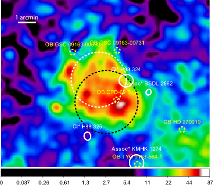
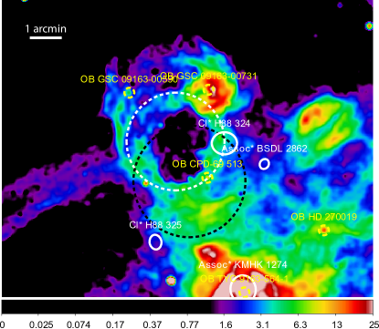
Figure 14: Stellar population in the DEM L299 region. Shown are OB-stars (yellow dashed small circles), clusters and associations of stars (white circles). The position of the remnant and of the superbubble are marked with a black and a white dashed circle. The images show the region in the broadband (0.3–8 keV) X-ray (left) and in the H$\alpha$ light (right). To create the images, the same parameters as in Figs. 2, left side, and 3, left side, have been used. Scales of the left image are in units of counts/s/deg², while the scales on the right side are in 10^-15 erg/cm²/s. The population study has been performed with SIMBAD.

with $R\approx R_{\mathrm{SB}}$ being the radius of the outer shell in cm, $E_{\mathrm{th,SB}}$ the thermal energy content of the superbubble in erg, $t_{\mathrm{dyn,SB}}$ the dynamic age of the superbubble in s, $\rho=n\,\mu\,m_{\mathrm{p}}$ is the mass density of all particles of the ambient medium in g/cm³, with the particle density $n$ of the ambient medium, the mean molecular mass $\mu$ and the proton mass $m_{\mathrm{p}}$. This is the same formula as given in Eq. 5, but this time with the coefficient $\alpha$ set to 0.76, according to a bubble in its intermediate stage (Weaver et al. 1977), in contrast to a coefficient of $2.02^{1/5}\approx 1.15$ used for the SNR. Solving this equation for $t_{\mathrm{dyn,SB}}$, we derive a dynamic age of $(70^{+73}_{-35})$ kyr for the superbubble, which is younger than the age found for other superbubbles. Considering the mass and thermal energy of the superbubble as determined above (without the blowout), this leads to an average mass-loss rate of $(1.9^{+3.9}_{-1.3})\times 10^{-3}$ M_☉/yr and an average energy input rate of $(2.0^{+4.3}_{-1.6})\times 10^{38}$ erg/s. However, this age seems too young with respect to the stellar ages of the stars that blew the superbubble. Such young ages for superbubbles have been found in other studies as well, for example by Sasaki et al. (2011) or Cooper et al. (2004). This might be explained by the growth rate discrepancy that has been observed in several superbubbles (e.g. Cooper et al. 2004; Jaskot et al. 2011). It states that, compared with the standard model of Weaver et al. (1977) for stellar bubbles and superbubbles, the growth rate of the superbubbles is too low regarding the stellar wind input. A discrepancy in the energy budget has been observed for superbubbles, since the thermal energy of the hot gas and the kinetic energy of the shells has been found to be too low to balance the energy input through stellar winds and supernovae (Cooper et al. 2004; Maddox et al. 2009). A possible explanation for this discrepancy is an energy loss of the superbubble through a blowout, as suggested for this superbubble through optical data. Other possible explanations are evaporation of cooler, denser cloudlets within the superbubble (e.g. Jaskot et al. 2011; Silich et al. 1996).

5.3 Input from stars

Table 5: OB-stars, associations of stars, and clusters of stars located within a radius of 4$\aas@@fstack{\prime}$5 from the centre of the SNR as defined by the [S II]/H$\alpha$ image. We have searched SIMBAD for the stellar populations in this area. We list the right ascension, declination, identifier and the type of each object. The last column indicates a possible physical connection as reported in Bica et al. (1999).

RA (J2000)	Dec (J2000)	Identifier	Type	Comments
05:42:54.93	-68:56:54.5	GSC 09163-00731	OB-star
05:43:24.67	-68:57:00.1	GSC 09163-00590	OB-star
05:42:55.414	-68:59:52.81	CPD-69 513	OB-star
05:42:11.561	-69:01:39.33	HD 270019	OB-star
05:42:41.496	-69:03:45.10	TYC 9163-564-1	OB-star
05:42:42	-69:03.7	KMHK 1274	Assoc. of stars	in LMC N-164
05:42:34	-68:59.4	BSDL 2862	Assoc. of stars
05:43:15	-69:02.0	H88 325	Cluster of stars
05:42:49	-68:58.7	H88 324	Cluster of stars	in DEM L299

We investigated the stellar population in the vicinity of DEM L299 to estimate the influence of the stellar population on the remnant and the superbubble emission. This influence can be a contribution to the X-ray flux through either OB-stars or low-mass stars for both objects, as well as energy input and mass input through supernova explosions and stellar winds for the superbubble.

For this purpose, a population study was performed with the SIMBAD astronomical database. Within a radius of 4$\aas@@fstack{\prime}$5 (65 pc) from the centre of the remnant as defined by the [S II]/H$\alpha$ image, we found five OB-stars, two clusters of stars, and two associations. These sources can be found in Table 5 and are plotted in Fig. 14, with the position and size of the clusters and associations as given in the catalogue of Bica et al. (1999). The association KMHK 1274, which is marked as possibly connected to LHA 120-N 164 by Bica et al. (1999), and the two OB-stars in the south-west of DEM L299 lie too far from the remnant (4′) and the superbubble (2′ and 3′) to be of much influence. One OB-star is projected towards DEM L299 at the north-western rim of the superbubble close to a star-forming region. The remaining two OB-stars, two clusters, and one association lie close to the borders of the remnant and/or the superbubble in projection, with one OB-star being inside the remnant. The cluster H88 324 was found to be possibly connected to DEM L299 by Bica et al. (1999). Unfortunately, no deeper study of this cluster or for the other cluster and association lying close to the superbubble could be found, and no further information about the spectral types of the OB-stars is listed in SIMBAD.

5.3.1 Energy and mass input for the superbubble

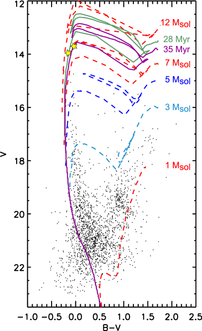
Figure 15: Colour-magnitude diagram for stars projected 2′ around the centre of the superbubble. Plotted are $\sim$ 1 900 stars from the photometric catalogue of Zaritsky et al. (2004). The dashed lines show the evolutionary tracks for stars with 1, 3 (light blue), 5 (dark blue), 7 and 12 M_☉ (marked in red if not stated differently, from bottom to top). The two most massive stars are marked with yellow star symbols. Two isochrones at 28 Myr (green) and 35 Myr (purple), which are taken from Lejeune & Schaerer (2001), are plotted as solid curves.

We estimated the energy and mass input of previous supernova explosions and stellar winds of massive stars to compare them with observed values. For this estimate, we needed the number of massive stars that were initially formed in this region, as well as the age of the stellar population. We used two different ways to estimate these numbers: via a colour-magnitude diagram, and via the software package Starburst99 (Leitherer et al. 1999; Vázquez & Leitherer 2005). This package allows model predictions for a variety of photometrical and spectral properties of a population of stars.

For the first method, we created a colour-magnitude diagram using the photometric catalogue of Zaritsky et al. (2004) for stars within a radius of 2′ (30 pc) around the centre of the superbubble. Figure 15 shows the resulting colour-magnitude diagram, including two isochrones at 28 Myr and 35 Myr (solid lines) as well as the evolutionary tracks for stars with an initial mass of 1, 3, 5, 7, and 12 M_☉ from Lejeune & Schaerer (2001). For these tracks, we chose the basic model set for the Johnson-Cousins-Glass photometry, calculated for a metallicity of Z=0.008, since this lies close to the metallicity of the LMC, which is about half of the solar value $Z_{\sun}$=0.02 (see Lejeune & Schaerer (2001) for more details about the evolutionary tracks and isochrones). In the diagram, $\sim$ 1 900 stars are plotted, with the most massive main-sequence stars having approximately 10 M_☉. Stars that are obviously separated from the main sequence but not at the turn-off point from the main sequence of the stellar population are considered as fore- and background stars and are therefore not taken into account.

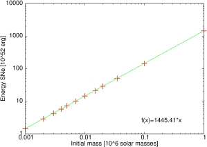
Figure 16: Logarithm of the energy input through supernovae as a function of the initial mass of the simulated stellar population with an age of 32 Myr. The simulation was made using Starburst99. Crosses are the simulation results and the dashed line is a fit to these values. This fitted function f(x) has been used to extrapolate to masses below the lower initial mass limit.

Assuming an IMF with a Salpeter power-law exponent of $\Gamma$=-1.35 (Salpeter 1955) in the mass range from 1–100 M_☉, we calculated the number of stars in the mass bin from 8–100 M_☉, with 8 M_☉ being the lower initial mass limit for a star to become a supernova. This was based on numbers in six different mass bins between 3–7 M_☉. We received an average number of 9${}^{+3}_{-3}$ stars for the mass bin from 8–100 M_☉. Since two stars lie above the evolutionary tracks for 8 M_☉ in the colour-magnitude diagram, we conclude that 7${}^{+3}_{-3}$ supernovae should have already occurred in the superbubble region.

We used the colour-magnitude diagram to determine the approximate age of the population. Since the two most massive stars, which lie between 7–12 M_☉ (marked with yellow star symbols), are both on or close to the main sequence, no turn-off point from the main sequence could be determined, but an upper age limit of 28–35 Myr can be inferred for the superbubble population, as indicated by the two plotted isochrones in Fig. 15. In addition, we determined the total initial mass for the stars between 1–100 M_☉ and obtained an average total mass of $(636^{+157}_{-158})\leavevmode\nobreak\$M_☉.

As a second way to determine the number of already occurred SNe, we used the Starburst99 v6.0.4 software and data package. As input parameters, we used the age and the total mass as obtained from the colour-magnitude diagram, a Salpeter IMF, and a metallicity of Z=0.008. Since Starburst99 was designed for simulating the population of whole galaxies, it has a lower initial mass limit of $1\times 10^{3}$ M_☉ and considers only masses in steps of $1\,000$ M_☉. Since our average initial mass of $\sim$ $640\leavevmode\nobreak\$M_☉ lies below the limit of Starburst99, we ran 12 different simulations with initial masses between $1\times 10^{3}$ M_☉ and $1\times 10^{6}$ M_☉ and extrapolated to our lower mass. We found that both the energy input and the total mass loss of the stars are a linear function of the mass (see Fig. 16 for the energy input of supernovae). We extrapolated an energy input through core-collapse supernovae of $\sim$ $(9.1^{+3.1}_{-3.1})\times 10^{51}$ erg (errors with respect to the upper and lower mass and time limits), leading to $\sim$ $9^{+3}_{-3}$ previous supernovae, assuming an energy input of $10^{51}$ erg per supernova. This large number of SNe and therefore a large energy input might be a result of uncertainties in the colour-magnitude diagram concerning the confusion with fore- and background stars and the error propagation of this to the input parameters for Starburst99. As a wind input, we derive $\sim$ $(1.6^{+0.4}_{-0.4})\times 10^{51}$ erg. For the total mass loss through supernovae and stellar winds, Starburst99 yields a value of approximately $(164^{+48}_{-46})\leavevmode\nobreak\$M_☉. This is similar to the mass that we found for the hot gas inside the superbubble, although the superbubble mass has a very high upper limit. Indeed, the superbubble mass is expected to be higher than the mass loss through stellar winds and supernovae, since evaporation of the swept-up shell (Silich et al. 1996) is an important mass contribution to the superbubble.

5.3.2 Stellar contribution to the X-ray luminosity

To estimate the X-ray luminosity of the superbubble and the SNR, we have to determine the amount of X-ray emission originating from stars in these regions that were not masked as point sources in our previous analysis. Within the fitting regions for the superbubble and the SNR, there are two catalogued OB-stars, one in each region. Since an O-star has an X-ray luminosity of typically $\sim$ $10^{31}$–$10^{33}$ erg s^-1 (Chlebowski et al. 1989; Berghoefer et al. 1997; Sana et al. 2006), the high-mass stars account for $\sim$ $2\times 10^{31}$–$2\times 10^{33}$ erg s^-1 of the X-ray luminosity of our X-ray spectra. The other stellar contribution of X-ray luminosity that has to be taken into account are low-mass stars between 0.008–3 M_☉. Although the X-ray luminosity of each of these low-mass stars is lower than that of an OB-star, these low-mass stars are so abundant that their X-ray emission might be observed as a diffuse emission (Oskinova 2005). Therefore, we have to know their number and average X-ray luminosity per mass bin to be able to estimate their fraction of diffuse emission in our X-ray images. To do so, we created a second colour-magnitude diagram for the area enclosed by a circle with a radius of 2′ around the centre of the superbubble and a circle around the SNR with a radius of 2$\aas@@fstack{\prime}$3. We obtained a value of $306^{+58}_{-58}$ low-mass stars. An estimate of the luminosity per star in a certain mass bin can be found by comparing our population with the population of the well-studied Orion nebula cluster (ONC), assuming that both populations differ only in their size and age and have the same IMF (for this method, see e.g. Getman et al. (2006); Ezoe et al. (2006); Broos et al. (2007); Kavanagh et al. (2012)). The Orion nebula cluster has been studied in great detail through the Chandra Orion Ultradeep Project (COUP, Getman et al. 2005). Using this COUP observation, Feigelson et al. (2005) determined the number of stars and the integrated luminosity per mass bin for the ONC as well as the relative contribution of each mass bin to the X-ray luminosity. For example, in the mass bin from 1–3 M_☉, they reported an integrated, unabsorbed luminosity in the energy band from 0.5–8 keV of $9.12\times 10^{32}$ erg s^-1, with 70 stars lying in this mass bin. Rescaling these values to the size of our stellar population, we used our upper limit of 364 stars in the 1–3 M_☉ bin and obtained an integrated luminosity of $4.7\times 10^{33}$ erg s^-1. According to Feigelson et al. (2005), the X-ray luminosity in this bin contributes 41 % of the total X-ray luminosity, while stars below 1 M_☉ account for another 33 %. Using these numbers, we obtain a total X-ray luminosity of $8.6\times 10^{33}$ erg s^-1 for our population of stars below 3 M_☉. Out of the colour-magnitude diagram, we determined an age of 28–35 Myr for the superbubble plus SNR population, which therefore seems to be older than the ONC population, for which Preibisch & Feigelson (2005) derived age estimates of $\lesssim$ 10 Myr for their star sample within the ONC, and Getman et al. (2005) stated that 80 % of the stars within 1 pc from the centre of the ONC are younger than 1 Myr. Since the X-ray luminosity of stars below 3 M_☉ decreases with time (see Preibisch & Feigelson 2005), the determined value for the X-ray luminosity of the low-mass stars can be considered as an upper limit. Compared with the X-ray luminosity of $1.79\times 10^{36}$ erg s^-1 in the same energy band from 0.5–8 keV that we obtained in Sect. 4 from our X-ray fits for the superbubble plus the SNR (i.e. for the polygonal superbubble-only and the SNR fitting-region), the X-ray luminosity of low-mass stars only accounts for $\sim$ 0.5 % of the diffuse X-ray emission in this region and can therefore be neglected in the context of this analysis.

6 Summary

We presented a multi-wavelength study of DEM L299 in the LMC. The morphological study of X-ray, optical, and radio data revealed that in addition to the supernova remnant SNR B0543-68.9, there is evidence for a superbubble. The position of the SNR (centre: RA 05:43:02.2, Dec -69:00:00.0 (J2000), radius: $\sim$ 30 pc) and the superbubble (centre: RA 05:43:07.4, Dec -68:58:39.3 (J2000), radius: $\sim$ 25 pc) were identified using the [S II]/H$\alpha$ flux-ratio image of the remnant and through a shell-like structure visible in the optical data for the superbubble. The two objects show diffuse X-ray emission, and a cold hydrogen shell-like structure is visible around both objects in H I data. The projection of the objects overlaps, with the superbubble lying slightly farther to the north. An indication for a blowout of the superbubble at its northern rim was found in the optical and X-ray data. We found an indication for a common hydrogen shell around the two objects, which means that they lie in the vicinity of each other, although the data are ambiguous. But since the DEM L299 region is located next to an active star formation region in the LMC and since the centre of the remnant is projected inside the superbubble, it seems likely that the two objects are connected and that the progenitor star of the SNR was part of the stellar association that formed the superbubble. Although there is evidence for a hydrogen shell, the data do not allow us to distinguish whether this is a common shell or two separate shells. Out of the radio continuum data, we found a spectral index of $\alpha=-0.34$ for the radio emission of SNR B0543-68.9. Since this index is rather flat, it indicates a dominance of the thermal emission and therefore a rather mature remnant, which was also found from the results of the X-ray spectral analysis.

In the X-ray spectral analysis, we fitted three different regions of DEM L299: a superbubble-only region, an SNR region that also contains superbubble emission, which we estimated through the fitting results of the superbubble-only region, and the blowout region north of the superbubble. For all three regions, the plane-parallel shock model vpshock gave the best fit results. We obtained a temperature $k_{\mathrm{B}}T$ for SNR B0543-68.9 of $(0.64^{+0.73}_{-0.20})$ keV, for the superbubble of $(0.74^{+0.36}_{-0.30})$ keV, and for the blowout of $(0.62^{+0.38}_{-0.42})$ keV, and determined the luminosities of the objects. Applying the Sedov solution, we used these results for the remnant to calculate its other properties, such as an age of $8.9^{+9.2}_{-5.4}$ kyr, a shock velocity of $(1\,200^{+1\,200}_{-700})$ km s^-1, a swept-up mass of $210\,(^{+150}_{-110})\leavevmode\nobreak\ \rm{M}_{\sun}$, and an initial energy of the explosion of $4.3\,(<14.0)\times 10^{51}$ erg. For the superbubble, we used the ideal gas equation to determine properties such as a pressure of $(9.5^{+17.2}_{-4.3})\times 10^{5}\,\phi^{-0.5}$ cm^-3 K, a mass of the hot gas inside the superbubble of $(130^{+230}_{-60})$ M_☉, a thermal energy content of $(4.3^{+8.1}_{-2.6})\times 10^{50}\,\phi^{0.5}$ erg of the hot gas, and a dynamic age of $(70^{+73}_{-35})$ kyr.

We estimated the influence from stars on our results by estimating their energy and mass input for the superbubble. Using the colour-magnitude diagram, we obtained a number of $(7^{+3}_{-3})$ past supernovae in the DEM L299 region and an age estimate of $\lesssim$28–35 Myr for the population that created the superbubble. We used Starburst99 to extrapolate the mass input through supernovae and stellar winds of $(164^{+48}_{-46})\leavevmode\nobreak\$M_☉, and an energy input of $\sim$ $(1.6^{+0.4}_{-0.4})\times 10^{51}$ erg through stellar winds and of $\sim$ $(9.1^{+3.1}_{-3.1})\times 10^{51}$ erg through supernovae. Thus, considering both results, we determined the number of already occurred supernovae in the DEM L299 region to be 4–12. Furthermore, we showed that the stellar X-ray contribution is negligible when estimating the diffuse X-ray emission of this region, since we found the high-mass and low-mass stars to account for only 0.6 % and 0.5 % of the diffuse emission.