Higgs \rightarrow μτ𝜇𝜏\mu\tau as an indication for S4subscript𝑆4S_{4} flavor symmetry

Miguel D. Campos Max-Planck-Institut für Kernphysik, Saupfercheckweg 1, 69117 Heidelberg, Germany    A. E. Cárcamo Hernández  Universidad Técnica Federico Santa María and Centro Científico-Tecnológico de Valparaíso
Casilla 110-V, Valparaíso, Chile
   H. Päs Fakultät für Physik, Technische Universität Dortmund, 44221 Dortmund, Germany    E. Schumacher Fakultät für Physik, Technische Universität Dortmund, 44221 Dortmund, Germany
Abstract

Lepton flavor violating Higgs decays can arise in flavor symmetry models where the Higgs sector is responsible for both the electroweak and the flavor symmetry breaking. Here we advocate an S4subscript𝑆4S_{4} three-Higgs-doublet model where tightly constrained flavor changing neutral currents are suppressed by a remnant Z3subscript𝑍3Z_{3} symmetry. A small breaking of this Z3subscript𝑍3Z_{3} symmetry can explain the 2.4σ2.4𝜎2.4\,\sigma excess of Higgs decay final states with a μτ𝜇𝜏\mu\tau topology reported recently by CMS if the new neutral scalars are light. The model also predicts sizable rates for lepton flavor violating Higgs decays in the eτ𝑒𝜏e\tau and eμ𝑒𝜇e\mu channels because of the unifying S4subscript𝑆4S_{4} flavor symmetry.

pacs:
11.30.Hv, 14.60.-z, 14.80.Ec
preprint: DO-TH 14/18

I Introduction

Lepton flavor violating (LFV) Higgs decays have been advocated as a harbinger of flavor symmetries explaining the large amount of lepton flavor mixing Bhattacharyya:2010hp ; Cao:2011df ; Bhattacharyya:2012ze ; Bhattacharyya:2012pi . Indeed, substantial LFV Higgs couplings can arise quite naturally in such models as a consequence of the maximal atmospheric μτ𝜇𝜏\mu-\tau mixing in the Pontecorvo-Maki-Nakagawa-Sakata (PMNS) matrix. To manifest itself in the physical mass basis, a misalignment of the Higgs doublets, typically utilized to yield a realistic symmetry breaking pattern, is necessary. While the scalar sector in Bhattacharyya:2010hp ; Cao:2011df ; Bhattacharyya:2012ze ; Bhattacharyya:2012pi decomposes into a Standard Model (SM)-like Higgs doublet and new exotic scalars experiencing LFV decays, in the following we present an S4subscript𝑆4S_{4} flavor model where these states mix, resulting in sizable LFV decays of the SM-like Higgs boson. This is particularly interesting after the recent report by the CMS Collaboration of a 2.4σ2.4𝜎2.4\,\sigma anomaly in the hμτ𝜇𝜏h\rightarrow\mu\tau channel with a best fit of Br(hμτ)0.84%𝜇𝜏percent0.84(h\rightarrow\mu\tau)\approx 0.84\% Khachatryan:2015kon , which as a possible hint of new physics beyond the SM, has drawn some attention Dery:2014kxa ; Lee:2014rba ; Celis:2014roa ; Sierra:2014nqa ; Heeck:2014qea ; Dorsner:2015mja ; Crivellin:2015lwa .

Notably, the discrete group S4subscript𝑆4S_{4} has been shown to be the most natural flavor symmetry of the tribimaximal (TBM) mixing scheme in the leptonic sector, with purely group theoretical arguments Hall:2013yha ; Bazzocchi:2012st ; Lam:2008sh , as well as in explicit flavor models Bazzocchi:2008ej ; Ishimori:2011mt ; Morisi:2010rk . Furthermore, together with the groups A4subscript𝐴4A_{4} and Δ(27)Δ27\Delta(27), the S4subscript𝑆4S_{4} group is the smallest group containing an irreducible triplet representation that can accommodate the three fermion families of the SM. Nonsupersymmetric S4subscript𝑆4S_{4} models based on TBM mixing but accommodating a large θ13subscript𝜃13\theta_{13} have been discussed e.g. in Krishnan:2012me ; Krishnan:2012sb ; Mohapatra:2012tb . To evade bounds from the tightly constrained radiative decays lαlβγsubscript𝑙𝛼subscript𝑙𝛽𝛾l_{\alpha}\rightarrow l_{\beta}\gamma, we consider the special case in which S4subscript𝑆4S_{4} is broken down to a residual Z3subscript𝑍3Z_{3} subgroup (see Cao:2011df in the context of the symmetry groups A4subscript𝐴4A_{4}, T7subscript𝑇7T_{7}, and Δ(27)Δ27\Delta(27), referred to as lepton flavor triality or LFT for short). This discrete Z3subscript𝑍3Z_{3} symmetry is obtained when scalar doublets in the irreducible triplet representation 𝟑superscript3\mathbf{3^{\prime}} of S4subscript𝑆4S_{4} assume the specific vacuum alignment (1,1,1)111(1,1,1) Bazzocchi:2008ej . If only the charged lepton sector is considered, the distinct Z3subscript𝑍3Z_{3} quantum numbers prevent any mixing of the physical scalars in this model. The Z3subscript𝑍3Z_{3} symmetry is, however, broken to some degree by perturbations arising from other scalar S4subscript𝑆4S_{4} triplets required to extend the model to quarks and neutrinos. These perturbations enable mixing between the scalars and consequently lead to LFV Higgs decays.

The measurement of hμτ𝜇𝜏h\rightarrow\mu\tau can be translated into a bound on the combination of Yukawa couplings |yμτ|2+|yτμ|2superscriptsubscript𝑦𝜇𝜏2superscriptsubscript𝑦𝜏𝜇2|y_{\mu\tau}|^{2}+|y_{\tau\mu}|^{2} Dorsner:2015mja . These couplings directly affect predictions for constrained LFV processes such as τμγ𝜏𝜇𝛾\tau\rightarrow\mu\gamma or τ3μ𝜏3𝜇\tau\rightarrow 3\mu which can be used to set bounds on the scalar masses in our 3HDM.

The paper is structured as follows. In Sec. II we develop a model with LFT that leads to realistic fermion masses and mixings. In Sec. III we analyze the breaking of the Z3subscript𝑍3Z_{3} group associated with LFT and its consequences for Higgs decays. In particular we focus on the hμτ𝜇𝜏h\rightarrow\mu\tau channel explaining the recent 2.4σ2.4𝜎2.4\,\sigma anomaly and summarize predictions of our model for other rare LFV processes. The hγγ𝛾𝛾h\rightarrow\gamma\gamma rate is considered in Sec. IV and a summary is given in Sec. V.

II The Model

II.1 Charged leptons

In the following we use the charged lepton sector as a starting point to introduce the relevant scalar content. Some of the additional scalars needed to accommodate quarks and neutrinos have an effect on the lepton phenomenology, which we can exploit to explain the excess in hμτ𝜇𝜏h\rightarrow\mu\tau reported by CMS, as will be discussed in Sec. III.
The particle assignments relevant for the charged lepton sector in the notation (S4,SU(2),Z12)subscript𝑆4𝑆𝑈2subscript𝑍12(S_{4},SU(2),Z_{12}) are

L=(Le,Lμ,Lτ):(3,2,1),:𝐿subscript𝐿𝑒subscript𝐿𝜇subscript𝐿𝜏superscript321\displaystyle L=(L_{e},L_{\mu},L_{\tau})\leavevmode\nobreak\ :\leavevmode\nobreak\ (3^{\prime},2,1)\,, τR:(1,1,i),(eR,μR):(2,1,e7iπ6),:subscript𝜏𝑅11𝑖subscript𝑒𝑅subscript𝜇𝑅:21superscript𝑒7𝑖𝜋6\displaystyle\tau_{R}\leavevmode\nobreak\ :\leavevmode\nobreak\ (1,1,-i)\,,\quad(e_{R},\mu_{R})\leavevmode\nobreak\ :\leavevmode\nobreak\ (2,1,e^{\frac{7i\pi}{6}})\,, (1)
ϕ=(ϕ1,ϕ2,ϕ3):(3,2,1),:italic-ϕsubscriptitalic-ϕ1subscriptitalic-ϕ2subscriptitalic-ϕ3superscript321\displaystyle\phi=(\phi_{1},\phi_{2},\phi_{3})\leavevmode\nobreak\ :\leavevmode\nobreak\ (3^{\prime},2,1)\,, η1:(1,1,eiπ6),η2:(1,1,eiπ6).:subscript𝜂111superscript𝑒𝑖𝜋6subscript𝜂2:superscript11superscript𝑒𝑖𝜋6\displaystyle\eta_{1}\leavevmode\nobreak\ :\leavevmode\nobreak\ (1,1,e^{\frac{i\pi}{6}}),\quad\eta_{2}\leavevmode\nobreak\ :\leavevmode\nobreak\ (1^{\prime},1,e^{\frac{i\pi}{6}})\,.

The scalar fields ϕjsubscriptitalic-ϕ𝑗\phi_{j} (j=1,2,3𝑗123j=1,2,3) and the left-handed fermion SU(2)𝑆𝑈2SU(2) doublets are both assigned to an S4subscript𝑆4S_{4} triplet representation 𝟑superscript3\mathbf{3^{\prime}}. The former break the electroweak (EW) symmetry of the SM by spontaneously acquiring VEVs at the EW scale. Such models are usually referred to as three-Higgs-doublet models (3HDMs) and have been extensively analyzed in the past, e.g., in Felipe:2013ie ; Keus:2013hya .

To describe the hierarchy among the charged fermion masses, we introduce two EW scalar singlets, η1subscript𝜂1\eta_{1} and η2subscript𝜂2\eta_{2}. For the VEVs of η1,2subscript𝜂12\eta_{1,2} we assume vη1,2=λΛsubscript𝑣subscript𝜂12𝜆Λv_{\eta_{1,2}}=\lambda\Lambda with λ0.22𝜆0.22\lambda\approx 0.22, where ΛΛ\Lambda is a high scale defining the breakdown of our effective theory. By choosing suitable Z12subscript𝑍12Z_{12} charges we ensure that the tau and muon mass arise from seven and nine dimensional Yukawa terms, respectively. The smallness of the electron mass on the other hand is explained by the destructive interference between the contributions coming from the nine dimensional Yukawa operators and by a small breaking of the universality of the corresponding Yukawa couplings. The Z12subscript𝑍12Z_{12}, therefore, functions as a Froggatt–Nielson-like symmetry by creating mass hierarchies in the lepton and quark sector with 𝒪(1)𝒪1\mathcal{O}(1) Yukawa couplings Wang:2011ub .

As a consequence of the particle assignments given in Eq. (1) the scalar potential V(ϕ)𝑉italic-ϕV(\phi) involving only the ϕitalic-ϕ\phi field is the general S4subscript𝑆4S_{4}-invariant scalar potential of a 3HDM Keus:2013hya . Since the singlet scalars are assumed to be very heavy, the mixing between ϕisubscriptitalic-ϕ𝑖\phi_{i} and η1,2subscript𝜂12\eta_{1,2} is suppressed. For simplicity we also assume a CP-conserving scalar potential with only real couplings as done in, e.g., Machado:2010uc . The renormalizable low-energy scalar potential is

V(ϕ)=𝑉italic-ϕabsent\displaystyle V(\phi)= μ12i=13ϕiϕi+α(i=13ϕiϕi)2+i,j=1,ij3(β(ϕiϕi)(ϕjϕj)+γ|ϕiϕj|2+δ(ϕiϕj)2)superscriptsubscript𝜇12superscriptsubscript𝑖13superscriptsubscriptitalic-ϕ𝑖subscriptitalic-ϕ𝑖𝛼superscriptsuperscriptsubscript𝑖13superscriptsubscriptitalic-ϕ𝑖subscriptitalic-ϕ𝑖2superscriptsubscriptformulae-sequence𝑖𝑗1𝑖𝑗3𝛽superscriptsubscriptitalic-ϕ𝑖subscriptitalic-ϕ𝑖superscriptsubscriptitalic-ϕ𝑗subscriptitalic-ϕ𝑗𝛾superscriptsuperscriptsubscriptitalic-ϕ𝑖subscriptitalic-ϕ𝑗2𝛿superscriptsuperscriptsubscriptitalic-ϕ𝑖subscriptitalic-ϕ𝑗2\displaystyle-\mu_{1}^{2}\sum_{i=1}^{3}\phi_{i}^{\dagger}\phi_{i}+\alpha\left(\sum_{i=1}^{3}\phi_{i}^{\dagger}\phi_{i}\right)^{2}+\sum_{i,j=1,i\neq j}^{3}(\beta(\phi_{i}^{\dagger}\phi_{i})(\phi_{j}^{\dagger}\phi_{j})+\gamma|\phi_{i}^{\dagger}\phi_{j}|^{2}+\delta(\phi_{i}^{\dagger}\phi_{j})^{2}) (2)

with the low-energy scalar content given by

ϕj=[ϕj+,12(v3+ϕjR0+iϕjI0)].subscriptitalic-ϕ𝑗matrixsuperscriptsubscriptitalic-ϕ𝑗12𝑣3subscriptsuperscriptitalic-ϕ0𝑗𝑅𝑖subscriptsuperscriptitalic-ϕ0𝑗𝐼\displaystyle\phi_{j}=\begin{bmatrix}{\phi_{j}^{+}},\quad{\frac{1}{\sqrt{2}}\left(\frac{v}{\sqrt{3}}+\phi^{0}_{jR}+i\phi^{0}_{jI}\right)}\end{bmatrix}. (3)

It includes three CP-even neutral scalars ϕjR0superscriptsubscriptitalic-ϕ𝑗𝑅0\phi_{jR}^{0} (j=1,2,3𝑗123j=1,2,3), and three CP-odd neutral scalars ϕjI0superscriptsubscriptitalic-ϕ𝑗𝐼0\phi_{jI}^{0}, as well as three complex charged scalars (ϕj+superscriptsubscriptitalic-ϕ𝑗\phi_{j}^{+}), of which three degrees of freedom are absorbed by the W±superscript𝑊plus-or-minusW^{\pm} and Z𝑍Z gauge boson masses. The corresponding physical mass spectrum reads

mϕ(a,b)R02=v23κ,mϕcR02=v23(3α+2κ),mϕ(a,b)I02=v2δ,mϕa,b±2=v2(κβ),mϕcI02=0,mϕc±2=0,subscriptsuperscript𝑚2subscriptsuperscriptitalic-ϕ0𝑎𝑏𝑅superscript𝑣23𝜅missing-subexpressionsubscriptsuperscript𝑚2subscriptsuperscriptitalic-ϕ0𝑐𝑅superscript𝑣233𝛼2𝜅missing-subexpressionsubscriptsuperscript𝑚2subscriptsuperscriptitalic-ϕ0𝑎𝑏𝐼superscript𝑣2𝛿subscriptsuperscript𝑚2subscriptsuperscriptitalic-ϕplus-or-minus𝑎𝑏superscript𝑣2𝜅𝛽missing-subexpressionsubscriptsuperscript𝑚2subscriptsuperscriptitalic-ϕ0𝑐𝐼0missing-subexpressionsubscriptsuperscript𝑚2subscriptsuperscriptitalic-ϕplus-or-minus𝑐0\begin{array}[]{rclcrclcrcl}m^{2}_{\phi^{0}_{(a,b)R}}&=&-\tfrac{v^{2}}{3}\kappa,&&m^{2}_{\phi^{0}_{cR}}&=&\tfrac{v^{2}}{3}(3\alpha+2\kappa),&&m^{2}_{\phi^{0}_{(a,b)I}}&=&-v^{2}\delta,\\ m^{2}_{\phi^{\pm}_{a,b}}&=&-v^{2}(\kappa-\beta),&&m^{2}_{\phi^{0}_{cI}}&=&0,&&m^{2}_{\phi^{\pm}_{c}}&=&0,\end{array} (4)

with κ:=β+γ+δassign𝜅𝛽𝛾𝛿\kappa:=\beta+\gamma+\delta.

The mass eigenstates ϕa,b,csubscriptitalic-ϕ𝑎𝑏𝑐\phi_{a,b,c} are given by the following linear combinations of the S4subscript𝑆4S_{4} basis scalars ϕ1,2,3subscriptitalic-ϕ123\phi_{1,2,3}:

ϕa=12(ϕ3ϕ2),ϕb=16(2ϕ1ϕ2ϕ3),ϕc=13(ϕ1+ϕ2+ϕ3).subscriptitalic-ϕ𝑎12subscriptitalic-ϕ3subscriptitalic-ϕ2missing-subexpressionsubscriptitalic-ϕ𝑏162subscriptitalic-ϕ1subscriptitalic-ϕ2subscriptitalic-ϕ3missing-subexpressionsubscriptitalic-ϕ𝑐13subscriptitalic-ϕ1subscriptitalic-ϕ2subscriptitalic-ϕ3\begin{array}[]{rclcrclcrcl}\phi_{a}&=&\frac{1}{\sqrt{2}}(\phi_{3}-\phi_{2}),&&\phi_{b}&=&\frac{1}{\sqrt{6}}(2\phi_{1}-\phi_{2}-\phi_{3}),&&\phi_{c}&=&\frac{1}{\sqrt{3}}(\phi_{1}+\phi_{2}+\phi_{3}).\end{array} (5)

These equations hold for the charged, CP-even and CP-odd components of ϕitalic-ϕ\phi, and they imply that

ϕa=ϕb=0andϕcformulae-sequencedelimited-⟨⟩subscriptitalic-ϕ𝑎delimited-⟨⟩subscriptitalic-ϕ𝑏0anddelimited-⟨⟩subscriptitalic-ϕ𝑐\displaystyle\langle\phi_{a}\rangle=\langle\phi_{b}\rangle=0\quad\text{and}\quad\langle\phi_{c}\rangle =v.absent𝑣\displaystyle=v. (6)

The fact that ϕcsubscriptitalic-ϕ𝑐\phi_{c} is the only mass eigenstate from the S4subscript𝑆4S_{4} triplet acquiring a VEV proves essential for LFT. Along with the degeneracy of the scalars ϕ(a,b)R0superscriptsubscriptitalic-ϕ𝑎𝑏𝑅0\phi_{(a,b)R}^{0} (cf. Eq. (4)), it suggests that ϕcR0superscriptsubscriptitalic-ϕ𝑐𝑅0\phi_{cR}^{0} can be identified as the SM Higgs particle found at the LHC with a mass of approximately 125 GeV.

Using Eq. (5) we obtain the three- and four-point vertices of the physical scalars and the gauge bosons W±,Z0superscript𝑊plus-or-minussuperscript𝑍0W^{\pm},Z^{0} and A𝐴A from the kinetic terms of the Lagrangian. In the case of the three-point interactions, the only induced decay channels are ϕcR0W+Wsubscriptsuperscriptitalic-ϕ0𝑐𝑅superscript𝑊superscript𝑊\phi^{0}_{cR}\to W^{+}W^{-} and ϕcR0(Z0)2subscriptsuperscriptitalic-ϕ0𝑐𝑅superscriptsuperscript𝑍02\phi^{0}_{cR}\to(Z^{0})^{2}. Hence, the SM-like Higgs ϕcR0superscriptsubscriptitalic-ϕ𝑐𝑅0\phi_{cR}^{0} is the only physical scalar giving masses to the SM gauge bosons with SM couplings. As a consequence, the masses of the neutral scalars ϕ(a,b)R0subscriptsuperscriptitalic-ϕ0𝑎𝑏𝑅\phi^{0}_{(a,b)R} are not constrained by the usual Higgs searches performed in the LEP and LHC experiments ATLAS-CONF-2012-019 ; CMS-PAS-HIG-12-008 .

The relevant S4Z12tensor-productsubscript𝑆4subscript𝑍12S_{4}\otimes Z_{12}-invariant Yukawa terms for the charged leptons

y1[Lϕ]1τRη13+ε0η1η22Λ3+y2[Lϕ]2(eRμR)η15+ε1η13η22+ε2η1η24Λ5+y3[Lϕ]2(eRμR)η25+ε3η23η12+ε4η2η14Λ5subscript𝑦1subscriptdelimited-[]𝐿italic-ϕ1subscript𝜏𝑅superscriptsubscript𝜂13subscript𝜀0subscript𝜂1superscriptsubscript𝜂22superscriptΛ3subscript𝑦2subscriptdelimited-[]𝐿italic-ϕ2subscript𝑒𝑅subscript𝜇𝑅superscriptsubscript𝜂15subscript𝜀1superscriptsubscript𝜂13superscriptsubscript𝜂22subscript𝜀2subscript𝜂1superscriptsubscript𝜂24superscriptΛ5subscript𝑦3subscriptdelimited-[]𝐿italic-ϕ2subscript𝑒𝑅subscript𝜇𝑅superscriptsubscript𝜂25subscript𝜀3superscriptsubscript𝜂23superscriptsubscript𝜂12subscript𝜀4subscript𝜂2superscriptsubscript𝜂14superscriptΛ5\mathcal{L}\supset y_{1}\left[L\phi\right]_{1}\tau_{R}\frac{\eta_{1}^{3}+\varepsilon_{0}\eta_{1}\eta_{2}^{2}}{\Lambda^{3}}+y_{2}\left[L\phi\right]_{2}\left(\begin{array}[]{c}e_{R}\\ \mu_{R}\end{array}\right)\frac{\eta_{1}^{5}+\varepsilon_{1}\eta_{1}^{3}\eta_{2}^{2}+\varepsilon_{2}\eta_{1}\eta_{2}^{4}}{\Lambda^{5}}+y_{3}\left[L\phi\right]_{2}\left(\begin{array}[]{c}e_{R}\\ \mu_{R}\end{array}\right)\frac{\eta_{2}^{5}+\varepsilon_{3}\eta_{2}^{3}\eta_{1}^{2}+\varepsilon_{4}\eta_{2}\eta_{1}^{4}}{\Lambda^{5}} (7)

lead to the following mass matrix for charged leptons:

Mlsubscript𝑀𝑙\displaystyle M_{l} =12(v1(y~2y~3)λ5v1(y~2+y~3)λ5v1y~1λ3v2ω2(y~2y~3)λ5v2ω(y~2+y~3)λ5v2y~1λ3v3ω(y~2y~3)λ5v3ω2(y~2+y~3)λ5v3y~1λ3)absent12subscript𝑣1subscript~𝑦2subscript~𝑦3superscript𝜆5subscript𝑣1subscript~𝑦2subscript~𝑦3superscript𝜆5subscript𝑣1subscript~𝑦1superscript𝜆3subscript𝑣2superscript𝜔2subscript~𝑦2subscript~𝑦3superscript𝜆5subscript𝑣2𝜔subscript~𝑦2subscript~𝑦3superscript𝜆5subscript𝑣2subscript~𝑦1superscript𝜆3subscript𝑣3𝜔subscript~𝑦2subscript~𝑦3superscript𝜆5subscript𝑣3superscript𝜔2subscript~𝑦2subscript~𝑦3superscript𝜆5subscript𝑣3subscript~𝑦1superscript𝜆3\displaystyle=\frac{1}{\sqrt{2}}\left(\begin{array}[]{ccc}v_{1}\left(\widetilde{y}_{2}-\widetilde{y}_{3}\right)\lambda^{5}&v_{1}\left(\widetilde{y}_{2}+\widetilde{y}_{3}\right)\lambda^{5}&v_{1}\widetilde{y}_{1}\lambda^{3}\\ v_{2}\omega^{2}\left(\widetilde{y}_{2}-\widetilde{y}_{3}\right)\lambda^{5}&v_{2}\omega\left(\widetilde{y}_{2}+\widetilde{y}_{3}\right)\lambda^{5}&v_{2}\widetilde{y}_{1}\lambda^{3}\\ v_{3}\omega\left(\widetilde{y}_{2}-\widetilde{y}_{3}\right)\lambda^{5}&v_{3}\omega^{2}\left(\widetilde{y}_{2}+\widetilde{y}_{3}\right)\lambda^{5}&v_{3}\widetilde{y}_{1}\lambda^{3}\end{array}\right) (11)
=v16(111ω2ω1ωω21)diag((y~2y~3)λ5,(y~2+y~3)λ5,y~1λ3)absent𝑣16111superscript𝜔2𝜔1𝜔superscript𝜔21diagsubscript~𝑦2subscript~𝑦3superscript𝜆5subscript~𝑦2subscript~𝑦3superscript𝜆5subscript~𝑦1superscript𝜆3\displaystyle=v\frac{1}{\sqrt{6}}\left(\begin{array}[]{ccc}1&1&1\\ \omega^{2}&\omega&1\\ \omega&\omega^{2}&1\end{array}\right)\text{diag}(\left(\widetilde{y}_{2}-\widetilde{y}_{3}\right)\lambda^{5},\left(\widetilde{y}_{2}+\widetilde{y}_{3}\right)\lambda^{5},\widetilde{y}_{1}\lambda^{3}) (15)

with v1=v2=v3=v3subscript𝑣1subscript𝑣2subscript𝑣3𝑣3v_{1}=v_{2}=v_{3}=\tfrac{v}{\sqrt{3}}, ω=e2iπ/3𝜔superscript𝑒2𝑖𝜋3\omega=e^{2i\pi/3} and y~1subscript~𝑦1\widetilde{y}_{1}, y~2subscript~𝑦2\widetilde{y}_{2}, y~3subscript~𝑦3\widetilde{y}_{3} given by

y~1=(1+ε0)y1,y~2=(1+ε1+ε2)y2,y~3=(1+ε3+ε4)y3,formulae-sequencesubscript~𝑦11subscript𝜀0subscript𝑦1formulae-sequencesubscript~𝑦21subscript𝜀1subscript𝜀2subscript𝑦2subscript~𝑦31subscript𝜀3subscript𝜀4subscript𝑦3\widetilde{y}_{1}=\left(1+\varepsilon_{0}\right)y_{1},\hskip 5.69046pt\hskip 5.69046pt\hskip 5.69046pt\hskip 5.69046pt\hskip 5.69046pt\hskip 5.69046pt\hskip 5.69046pt\widetilde{y}_{2}=\left(1+\varepsilon_{1}+\varepsilon_{2}\right)y_{2},\hskip 5.69046pt\hskip 5.69046pt\hskip 5.69046pt\hskip 5.69046pt\hskip 5.69046pt\hskip 5.69046pt\hskip 5.69046pt\widetilde{y}_{3}=\left(1+\varepsilon_{3}+\varepsilon_{4}\right)y_{3}, (16)

where the dimensionless couplings y1subscript𝑦1y_{1}, y2subscript𝑦2y_{2}, y3subscript𝑦3y_{3}, ε0subscript𝜀0\varepsilon_{0}, ε1subscript𝜀1\varepsilon_{1}, ε2subscript𝜀2\varepsilon_{2}, ε3subscript𝜀3\varepsilon_{3} and ε4subscript𝜀4\varepsilon_{4} are 𝒪(1)𝒪1\mathcal{O}(1) parameters. Consequently the charged lepton masses are

me=(y~2y~3)λ5v2,mμ=(y~2+y~3)λ5v2,mτ=y~1λ3v2.formulae-sequencesubscript𝑚𝑒subscript~𝑦2subscript~𝑦3superscript𝜆5𝑣2formulae-sequencesubscript𝑚𝜇subscript~𝑦2subscript~𝑦3superscript𝜆5𝑣2subscript𝑚𝜏subscript~𝑦1superscript𝜆3𝑣2m_{e}=\left(\widetilde{y}_{2}-\widetilde{y}_{3}\right)\lambda^{5}\frac{v}{\sqrt{2}},\hskip 5.69046pt\hskip 5.69046pt\hskip 5.69046pt\hskip 5.69046pt\hskip 5.69046pt\hskip 5.69046pt\hskip 5.69046ptm_{\mu}=\left(\widetilde{y}_{2}+\widetilde{y}_{3}\right)\lambda^{5}\frac{v}{\sqrt{2}},\hskip 5.69046pt\hskip 5.69046pt\hskip 5.69046pt\hskip 5.69046pt\hskip 5.69046pt\hskip 5.69046pt\hskip 5.69046ptm_{\tau}=\widetilde{y}_{1}\lambda^{3}\frac{v}{\sqrt{2}}. (17)

The mass hierarchy me,mμmτmuch-less-thansubscript𝑚𝑒subscript𝑚𝜇subscript𝑚𝜏m_{e},m_{\mu}\ll m_{\tau}, therefore, is a natural consequence of our model.

Equation (11) shows a characteristic feature of LFT that the mass basis of the charged leptons coincides with the Z3subscript𝑍3Z_{3} basis; i.e., the charged lepton fields can be identified as Z3subscript𝑍3Z_{3} eigenstates e1,μω2,τωformulae-sequencesimilar-to𝑒1formulae-sequencesimilar-to𝜇superscript𝜔2similar-to𝜏𝜔e\sim 1,\mu\sim\omega^{2},\tau\sim\omega.

The structures for the couplings of the charged leptons to the physical scalars ϕaR0,ϕbR0subscriptsuperscriptitalic-ϕ0𝑎𝑅subscriptsuperscriptitalic-ϕ0𝑏𝑅\phi^{0}_{aR},\phi^{0}_{bR} and ϕcR0subscriptsuperscriptitalic-ϕ0𝑐𝑅\phi^{0}_{cR} are given by

Y(a)b=(i)1v2(0mμω2()mτω()meω0mτω2meω2()mμω0),Yc=1v(me000mμ000mτ),formulae-sequencesubscript𝑌𝑎𝑏𝑖1𝑣20subscript𝑚𝜇superscript𝜔2subscript𝑚𝜏𝜔subscript𝑚𝑒𝜔0subscript𝑚𝜏superscript𝜔2subscript𝑚𝑒superscript𝜔2subscript𝑚𝜇𝜔0subscript𝑌𝑐1𝑣subscript𝑚𝑒000subscript𝑚𝜇000subscript𝑚𝜏\displaystyle Y_{(a)b}=(i)\frac{1}{v\sqrt{2}}\left(\begin{array}[]{ccc}0&m_{\mu}\omega^{2}&(-)m_{\tau}\omega\\ (-)m_{e}\omega&0&m_{\tau}\omega^{2}\\ m_{e}\omega^{2}&(-)m_{\mu}\omega&0\end{array}\right),\quad Y_{c}=\frac{1}{v}\left(\begin{array}[]{ccc}m_{e}&0&0\\ 0&m_{\mu}&0\\ 0&0&m_{\tau}\end{array}\right), (24)

where the factors in parentheses apply only to the structure of Yasubscript𝑌𝑎Y_{a}. As can be seen from Eq. (24), ϕcsubscriptitalic-ϕ𝑐\phi_{c} only couples diagonally to the charged leptons and, hence, should be uncharged under Z3subscript𝑍3Z_{3}. This can be understood by expressing the fields ϕa,b,csubscriptitalic-ϕ𝑎𝑏𝑐\phi_{a,b,c} in terms of the Z3subscript𝑍3Z_{3} eigenstates

(ϕxϕyϕz)=13(1111ω2ω1ωω2)(ϕ1ϕ2ϕ3)withϕx,y,z1,ω,ω2formulae-sequencesubscriptitalic-ϕ𝑥subscriptitalic-ϕ𝑦subscriptitalic-ϕ𝑧131111superscript𝜔2𝜔1𝜔superscript𝜔2subscriptitalic-ϕ1subscriptitalic-ϕ2subscriptitalic-ϕ3withsimilar-tosubscriptitalic-ϕ𝑥𝑦𝑧1𝜔superscript𝜔2\displaystyle\left(\begin{array}[]{c}\phi_{x}\\ \phi_{y}\\ \phi_{z}\end{array}\right)=\frac{1}{\sqrt{3}}\left(\begin{array}[]{ccc}1&1&1\\ 1&\omega^{2}&\omega\\ 1&\omega&\omega^{2}\end{array}\right)\left(\begin{array}[]{c}\phi_{1}\\ \phi_{2}\\ \phi_{3}\end{array}\right)\qquad\text{with}\quad\phi_{x,y,z}\sim 1,\omega,\omega^{2} (34)

and consequently realizing that

ϕcϕx,ϕb12(ϕy+ϕz),ϕa12(ϕyϕz).formulae-sequencesubscriptitalic-ϕ𝑐subscriptitalic-ϕ𝑥formulae-sequencesubscriptitalic-ϕ𝑏12subscriptitalic-ϕ𝑦subscriptitalic-ϕ𝑧subscriptitalic-ϕ𝑎12subscriptitalic-ϕ𝑦subscriptitalic-ϕ𝑧\displaystyle\phi_{c}\equiv\phi_{x},\qquad\phi_{b}\equiv\frac{1}{\sqrt{2}}(\phi_{y}+\phi_{z}),\qquad\phi_{a}\equiv\frac{1}{\sqrt{2}}(\phi_{y}-\phi_{z}). (35)

Considering that ϕcsubscriptitalic-ϕ𝑐\phi_{c} is the only mass eigenstate from the ϕitalic-ϕ\phi S4subscript𝑆4S_{4} triplet that acquires a VEV (cf. Eq. (6)), Z3subscript𝑍3Z_{3} remains unbroken at this point.

II.2 Neutrino sector

To generate the neutrino masses via a type I seesaw mechanism, we extend the SM particle content by two heavy Majorana neutrinos N1Rsubscript𝑁1𝑅N_{1R} and N2Rsubscript𝑁2𝑅N_{2R} as well as four S4subscript𝑆4S_{4} triplets scalar fields χ𝜒\chi, ξ𝜉\xi, σ𝜎\sigma and ζ𝜁\zeta, which are singlets under SU(2)𝑆𝑈2SU(2). Additionally we employ two Z2subscript𝑍2Z_{2} symmetries to enforce a specific mass pattern and decouple the scalars from interactions with the other fermion sectors. The corresponding S4Z2Z2Z12tensor-productsubscript𝑆4subscript𝑍2superscriptsubscript𝑍2subscript𝑍12S_{4}\otimes Z_{2}\otimes Z_{2}^{\prime}\otimes Z_{12} assignments are

N1R:(1,1,1,1),N2R:(1,1,1,1),:subscript𝑁1𝑅1111subscript𝑁2𝑅:1111\displaystyle N_{1R}\leavevmode\nobreak\ :\leavevmode\nobreak\ (1,-1,1,1)\,,\quad N_{2R}\leavevmode\nobreak\ :\leavevmode\nobreak\ (1,-1,-1,1), (36)
χ:(3,1,1,1):𝜒superscript3111\displaystyle\chi:\leavevmode\nobreak\ (3^{\prime},-1,1,1) ,ξ:(3,1,1,1),σ:(3,1,1,1),ζ:(3,1,1,1).\displaystyle\,,\quad\xi\leavevmode\nobreak\ :\leavevmode\nobreak\ (3,-1,1,1)\,,\quad\sigma:\leavevmode\nobreak\ (3^{\prime},-1,-1,1)\,,\quad\zeta:\leavevmode\nobreak\ (3,-1,-1,1).

Therefore the relevant S4Z2Z2Z12tensor-productsubscript𝑆4subscript𝑍2superscriptsubscript𝑍2subscript𝑍12S_{4}\otimes Z_{2}\otimes Z_{2}^{\prime}\otimes Z_{12} -invariant neutrino Yukawa terms read

\displaystyle\mathcal{L} superset-of\displaystyle\supset y1(ν)[Lϕ]3N1RχΛ+y2(ν)[Lϕ]3N1RξΛ+y3(ν)[Lϕ]3N2RσΛ+y4(ν)[Lϕ]3N2RζΛ+y5(ν)ΛL[ϕχ]3N1Rsuperscriptsubscript𝑦1𝜈subscriptdelimited-[]𝐿italic-ϕsuperscript3subscript𝑁1𝑅𝜒Λsuperscriptsubscript𝑦2𝜈subscriptdelimited-[]𝐿italic-ϕ3subscript𝑁1𝑅𝜉Λsuperscriptsubscript𝑦3𝜈subscriptdelimited-[]𝐿italic-ϕsuperscript3subscript𝑁2𝑅𝜎Λsuperscriptsubscript𝑦4𝜈subscriptdelimited-[]𝐿italic-ϕ3subscript𝑁2𝑅𝜁Λsuperscriptsubscript𝑦5𝜈Λ𝐿subscriptdelimited-[]italic-ϕ𝜒superscript3subscript𝑁1𝑅\displaystyle y_{1}^{\left(\nu\right)}\left[L\phi\right]_{3^{\prime}}N_{1R}\leavevmode\nobreak\ \frac{\chi}{\Lambda}+y_{2}^{\left(\nu\right)}\left[L\phi\right]_{3}N_{1R}\leavevmode\nobreak\ \frac{\xi}{\Lambda}+y_{3}^{\left(\nu\right)}\left[L\phi\right]_{3^{\prime}}N_{2R}\leavevmode\nobreak\ \frac{\sigma}{\Lambda}+y_{4}^{\left(\nu\right)}\left[L\phi\right]_{3}N_{2R}\leavevmode\nobreak\ \frac{\zeta}{\Lambda}+\frac{y_{5}^{\left(\nu\right)}}{\Lambda}L\left[\phi\chi\right]_{3^{\prime}}N_{1R}\leavevmode\nobreak\ (37)
+y6(ν)ΛL[ϕξ]3N1R+y7(ν)ΛL[ϕσ]3N2R+y8(ν)ΛL[ϕζ]3N2R+M1N¯1RN1Rc+M2N¯2RN2Rc.superscriptsubscript𝑦6𝜈Λ𝐿subscriptdelimited-[]italic-ϕ𝜉superscript3subscript𝑁1𝑅superscriptsubscript𝑦7𝜈Λ𝐿subscriptdelimited-[]italic-ϕ𝜎superscript3subscript𝑁2𝑅superscriptsubscript𝑦8𝜈Λ𝐿subscriptdelimited-[]italic-ϕ𝜁superscript3subscript𝑁2𝑅subscript𝑀1subscript¯𝑁1𝑅superscriptsubscript𝑁1𝑅𝑐subscript𝑀2subscript¯𝑁2𝑅superscriptsubscript𝑁2𝑅𝑐\displaystyle+\frac{y_{6}^{\left(\nu\right)}}{\Lambda}L\left[\phi\xi\right]_{3^{\prime}}N_{1R}+\frac{y_{7}^{\left(\nu\right)}}{\Lambda}L\left[\phi\sigma\right]_{3^{\prime}}N_{2R}+\frac{y_{8}^{\left(\nu\right)}}{\Lambda}L\left[\phi\zeta\right]_{3^{\prime}}N_{2R}+M_{1}\overline{N}_{1R}N_{1R}^{c}+M_{2}\overline{N}_{2R}N_{2R}^{c}.

With the VEV patterns of the scalar fields χ𝜒\chi, ξ𝜉\xi, σ𝜎\sigma and ζ𝜁\zeta

χ=vχ(1,0,0),ξ=vξ(1,0,0),σ=vσ(0,i,0),ζ=vζ(0,1,0)formulae-sequencedelimited-⟨⟩𝜒subscript𝑣𝜒100formulae-sequencedelimited-⟨⟩𝜉subscript𝑣𝜉100formulae-sequencedelimited-⟨⟩𝜎subscript𝑣𝜎0𝑖0delimited-⟨⟩𝜁subscript𝑣𝜁010\left\langle\chi\right\rangle=v_{\chi}\left(1,0,0\right)\,,\quad\left\langle\xi\right\rangle=v_{\xi}\left(1,0,0\right)\,,\quad\left\langle\sigma\right\rangle=v_{\sigma}\left(0,i,0\right)\,,\quad\left\langle\zeta\right\rangle=v_{\zeta}\left(0,1,0\right)\,\, (38)

and the simplification

y1(ν)=y2(ν)=y5(ν)=y6(ν)=y(ν),superscriptsubscript𝑦1𝜈superscriptsubscript𝑦2𝜈superscriptsubscript𝑦5𝜈superscriptsubscript𝑦6𝜈superscript𝑦𝜈y_{1}^{\left(\nu\right)}=y_{2}^{\left(\nu\right)}=y_{5}^{\left(\nu\right)}=y_{6}^{\left(\nu\right)}=y^{\left(\nu\right)}\,, (39)

it follows that the full 5×5555\times 5 neutrino mass matrix is

ML(ν)=(03×3MνD(MνD)TMR),superscriptsubscript𝑀𝐿𝜈subscript033superscriptsubscript𝑀𝜈𝐷superscriptsuperscriptsubscript𝑀𝜈𝐷𝑇subscript𝑀𝑅M_{L}^{\left(\nu\right)}=\left(\begin{array}[]{cc}0_{3\times 3}&M_{\nu}^{D}\\ \left(M_{\nu}^{D}\right)^{T}&M_{R}\end{array}\right), (40)

where

MνDsuperscriptsubscript𝑀𝜈𝐷\displaystyle M_{\nu}^{D} =\displaystyle= (0λ[(y4(ν)+y6(ν))i(y3(ν)+y7(ν))]4λy(ν)00λ[(y4(ν)+y6(ν))+i(y3(ν)+y7(ν))])v3=(0aeiτb00aeiτ)v3,MR=(M100M2),formulae-sequence0𝜆delimited-[]superscriptsubscript𝑦4𝜈superscriptsubscript𝑦6𝜈𝑖superscriptsubscript𝑦3𝜈superscriptsubscript𝑦7𝜈4𝜆superscript𝑦𝜈00𝜆delimited-[]superscriptsubscript𝑦4𝜈superscriptsubscript𝑦6𝜈𝑖superscriptsubscript𝑦3𝜈superscriptsubscript𝑦7𝜈𝑣30𝑎superscript𝑒𝑖𝜏𝑏00𝑎superscript𝑒𝑖𝜏𝑣3subscript𝑀𝑅subscript𝑀100subscript𝑀2\displaystyle\left(\begin{array}[]{cc}0&\lambda\left[\left(y_{4}^{\left(\nu\right)}+y_{6}^{\left(\nu\right)}\right)-i\left(y_{3}^{\left(\nu\right)}+y_{7}^{\left(\nu\right)}\right)\right]\\ 4\lambda y^{\left(\nu\right)}&0\\ 0&\lambda\left[\left(y_{4}^{\left(\nu\right)}+y_{6}^{\left(\nu\right)}\right)+i\left(y_{3}^{\left(\nu\right)}+y_{7}^{\left(\nu\right)}\right)\right]\end{array}\right)\frac{v}{\sqrt{3}}=\left(\begin{array}[]{cc}0&ae^{i\tau}\\ b&0\\ 0&ae^{-i\tau}\end{array}\right)\frac{v}{\sqrt{3}},\hskip 28.45274ptM_{R}=\left(\begin{array}[]{cc}M_{1}&0\\ 0&M_{2}\end{array}\right), (49)
a𝑎\displaystyle a =\displaystyle= λ(y4(ν)+y6(ν))2+(y3(ν)+y7(ν))2,b=4λy(ν),tanτ=y3(ν)+y7(ν)y4(ν)+y6(ν).formulae-sequence𝜆superscriptsuperscriptsubscript𝑦4𝜈superscriptsubscript𝑦6𝜈2superscriptsuperscriptsubscript𝑦3𝜈superscriptsubscript𝑦7𝜈2𝑏4𝜆superscript𝑦𝜈𝜏superscriptsubscript𝑦3𝜈superscriptsubscript𝑦7𝜈superscriptsubscript𝑦4𝜈superscriptsubscript𝑦6𝜈\displaystyle\lambda\sqrt{\left(y_{4}^{\left(\nu\right)}+y_{6}^{\left(\nu\right)}\right)^{2}+\left(y_{3}^{\left(\nu\right)}+y_{7}^{\left(\nu\right)}\right)^{2}},\hskip 28.45274pt\hskip 28.45274ptb=4\lambda y^{\left(\nu\right)},\hskip 28.45274pt\hskip 28.45274pt\tan\tau=-\frac{y_{3}^{\left(\nu\right)}+y_{7}^{\left(\nu\right)}}{y_{4}^{\left(\nu\right)}+y_{6}^{\left(\nu\right)}}. (50)

Since (MR)iivmuch-greater-thansubscriptsubscript𝑀𝑅𝑖𝑖𝑣\left(M_{R}\right)_{ii}\gg v, the light neutrino mass matrix arises from a type I seesaw mechanism and is given by:

ML(ν)=MνDMR1(MνD)T=(a2e2iτ0a20b2M2M10a20a2e2iτ)v23M2=(Ae2iτ0A0B0A0Ae2iτ)superscriptsubscript𝑀𝐿𝜈superscriptsubscript𝑀𝜈𝐷superscriptsubscript𝑀𝑅1superscriptsuperscriptsubscript𝑀𝜈𝐷𝑇superscript𝑎2superscript𝑒2𝑖𝜏0superscript𝑎20superscript𝑏2subscript𝑀2subscript𝑀10superscript𝑎20superscript𝑎2superscript𝑒2𝑖𝜏superscript𝑣23subscript𝑀2𝐴superscript𝑒2𝑖𝜏0𝐴0𝐵0𝐴0𝐴superscript𝑒2𝑖𝜏M_{L}^{\left(\nu\right)}=M_{\nu}^{D}M_{R}^{-1}\left(M_{\nu}^{D}\right)^{T}=\left(\begin{array}[]{ccc}a^{2}e^{2i\tau}&0&a^{2}\\ 0&b^{2}\frac{M_{2}}{M_{1}}&0\\ a^{2}&0&a^{2}e^{-2i\tau}\end{array}\right)\frac{v^{2}}{3M_{2}}=\left(\begin{array}[]{ccc}Ae^{2i\tau}&0&A\\ 0&B&0\\ A&0&Ae^{-2i\tau}\end{array}\right) (51)

with

A=a2v23M2,B=b2v23M1.formulae-sequence𝐴superscript𝑎2superscript𝑣23subscript𝑀2𝐵superscript𝑏2superscript𝑣23subscript𝑀1A=a^{2}\frac{v^{2}}{3M_{2}},\hskip 5.69046pt\hskip 5.69046pt\hskip 5.69046pt\hskip 5.69046pt\hskip 5.69046pt\hskip 5.69046pt\hskip 5.69046ptB=b^{2}\frac{v^{2}}{3M_{1}}. (52)

It is worth mentioning that the neutrino mass matrix depends only on three effective parameters, A,B𝐴𝐵A,B and τ𝜏\tau, of which A𝐴A and B𝐵B are inverse proportional to M2subscript𝑀2M_{2} and M1subscript𝑀1M_{1}, respectively. Furthermore, the smallness of the active neutrino masses arises from their inverse scaling with the large Majorana neutrino masses as well as from the quadratic dependence of the neutrino Yukawa couplings, which is a characteristic feature of the type I seesaw mechanism. The right handed Majorana neutrinos obtain large masses due to their Yukawa interactions with EW scalar singlets, which acquire VEVs much larger than the electroweak scale.

The squared mass matrix ML(ν)(ML(ν))superscriptsubscript𝑀𝐿𝜈superscriptsuperscriptsubscript𝑀𝐿𝜈M_{L}^{\left(\nu\right)}\left(M_{L}^{\left(\nu\right)}\right)^{\dagger} is diagonalized by a unitary rotation matrix Vνsubscript𝑉𝜈V_{\nu} as follows Hernandez:2013dta ; Campos:2014lla ; Hernandez:2015tna ; Hernandez:2015cra :

VνMν(1)(Mν(1))Vν=(m12000m22000m32),withVν=(cosψ0sinψeiϕ010sinψeiϕ0cosψ),ψ=±π4,ϕ=2τ,formulae-sequencesuperscriptsubscript𝑉𝜈superscriptsubscript𝑀𝜈1superscriptsuperscriptsubscript𝑀𝜈1subscript𝑉𝜈superscriptsubscript𝑚12000superscriptsubscript𝑚22000superscriptsubscript𝑚32withformulae-sequencesubscript𝑉𝜈𝜓0𝜓superscript𝑒𝑖italic-ϕ010𝜓superscript𝑒𝑖italic-ϕ0𝜓formulae-sequence𝜓plus-or-minus𝜋4italic-ϕ2𝜏V_{\nu}^{\dagger}M_{\nu}^{\left(1\right)}\left(M_{\nu}^{\left(1\right)}\right)^{\dagger}V_{\nu}=\left(\begin{array}[]{ccc}m_{1}^{2}&0&0\\ 0&m_{2}^{2}&0\\ 0&0&m_{3}^{2}\end{array}\right),\hskip 14.22636pt\mbox{with}\hskip 14.22636ptV_{\nu}=\left(\begin{array}[]{ccc}\cos\psi&0&\sin\psi e^{-i\phi}\\ 0&1&0\\ -\sin\psi e^{i\phi}&0&\cos\psi\end{array}\right),\hskip 14.22636pt\psi=\pm\frac{\pi}{4},\hskip 14.22636pt\phi=-2\tau, (53)

where ψ=+π/4𝜓𝜋4\psi=+\pi/4 and ψ=π/4𝜓𝜋4\psi=-\pi/4 correspond to the normal (NH) and inverted (IH) mass hierarchies, respectively. The light active neutrino masses for NH and IH are:

NH ::\displaystyle: ψ=+π4:mν1=0,mν2=B,mν3=2|A|,\displaystyle\psi=+\frac{\pi}{4}:\hskip 28.45274ptm_{\nu_{1}}=0,\hskip 28.45274ptm_{\nu_{2}}=B,\hskip 28.45274ptm_{\nu_{3}}=2\left|A\right|, (54)
IH ::\displaystyle: ψ=π4:mν1=2|A|,mν2=B,mν3=0.\displaystyle\psi=-\frac{\pi}{4}:\hskip 28.45274ptm_{\nu_{1}}=2\left|A\right|,\hskip 22.76219ptm_{\nu_{2}}=B,\hskip 28.45274ptm_{\nu_{3}}=0. (55)

By combining Eqs. (11) and (53) we obtain the PMNS leptonic mixing matrix

U=VlLVν=(cosψ3eiϕ2iπ3sinψ3e2iπ33e2iπ3cosψ3+eiϕsinψ3cosψ3eiϕ+2iπ3sinψ3e2iπ33e2iπ3cosψ3+eiϕsinψ3cosψ3eiϕsinψ313cosψ3+eiϕsinψ3),𝑈superscriptsubscript𝑉𝑙𝐿subscript𝑉𝜈𝜓3superscript𝑒𝑖italic-ϕ2𝑖𝜋3𝜓3superscript𝑒2𝑖𝜋33superscript𝑒2𝑖𝜋3𝜓3superscript𝑒𝑖italic-ϕ𝜓3missing-subexpressionmissing-subexpressionmissing-subexpression𝜓3superscript𝑒𝑖italic-ϕ2𝑖𝜋3𝜓3superscript𝑒2𝑖𝜋33superscript𝑒2𝑖𝜋3𝜓3superscript𝑒𝑖italic-ϕ𝜓3missing-subexpressionmissing-subexpressionmissing-subexpression𝜓3superscript𝑒𝑖italic-ϕ𝜓313𝜓3superscript𝑒𝑖italic-ϕ𝜓3U=V_{lL}^{{\dagger}}V_{\nu}=\left(\begin{array}[]{ccc}\frac{\cos\psi}{\sqrt{3}}-\frac{e^{i\phi-\frac{2i\pi}{3}}\sin\psi}{\sqrt{3}}&\frac{e^{\frac{2i\pi}{3}}}{\sqrt{3}}&\frac{e^{-\frac{2i\pi}{3}}\cos\psi}{\sqrt{3}}+\frac{e^{-i\phi}\sin\psi}{\sqrt{3}}\\ &&\\ \frac{\cos\psi}{\sqrt{3}}-\frac{e^{i\phi+\frac{2i\pi}{3}}\sin\psi}{\sqrt{3}}&\frac{e^{-\frac{2i\pi}{3}}}{\sqrt{3}}&\frac{e^{\frac{2i\pi}{3}}\cos\psi}{\sqrt{3}}+\frac{e^{-i\phi}\sin\psi}{\sqrt{3}}\\ &&\\ \frac{\cos\psi}{\sqrt{3}}-\frac{e^{i\phi}\sin\psi}{\sqrt{3}}&\frac{1}{\sqrt{3}}&\frac{\cos\psi}{\sqrt{3}}+\frac{e^{-i\phi}\sin\psi}{\sqrt{3}}\end{array}\right), (56)

which only depends on a single parameter ϕitalic-ϕ\phi, whereas the neutrino mass squared splittings are determined by the parameters A𝐴A and B𝐵B.

Furthermore, we find that the lepton mixing angles are given by:

sin2θ12=|Ue2|21|Ue3|2=24±(cosϕ3sinϕ),superscript2subscript𝜃12superscriptsubscript𝑈𝑒221superscriptsubscript𝑈𝑒322plus-or-minus4italic-ϕ3italic-ϕ\displaystyle\sin^{2}\theta_{12}=\frac{\left|U_{e2}\right|^{2}}{1-\left|U_{e3}\right|^{2}}=\frac{2}{4\pm\left(\cos\phi-\sqrt{3}\sin\phi\right)},\hskip 56.9055pt (57)
sin2θ13=|Ue3|2=16[2(cosϕ3sinϕ)],superscript2subscript𝜃13superscriptsubscript𝑈𝑒3216delimited-[]minus-or-plus2italic-ϕ3italic-ϕ\displaystyle\sin^{2}\theta_{13}=\left|U_{e3}\right|^{2}=\frac{1}{6}\left[2\mp(\cos\phi-\sqrt{3}\sin\phi)\right], (58)
sin2θ23=|Uμ3|21|Ue3|2=2(cosϕ+3sinϕ)4±(cosϕ3sinϕ).superscript2subscript𝜃23superscriptsubscript𝑈𝜇321superscriptsubscript𝑈𝑒32minus-or-plus2italic-ϕ3italic-ϕplus-or-minus4italic-ϕ3italic-ϕ\displaystyle\sin^{2}\theta_{23}=\frac{\left|U_{\mu 3}\right|^{2}}{1-\left|U_{e3}\right|^{2}}=\frac{2\mp(\cos\phi+\sqrt{3}\sin\phi)}{4\pm\left(\cos\phi-\sqrt{3}\sin\phi\right)}. (59)

The Jarlskog invariant and the CP-violating phase are given by PDG-2014

J=Im(Ue1Uμ2Ue2Uμ1)=163cos2ψ,sinδ=8Jcosθ13sin2θ12sin2θ23sin2θ13.formulae-sequence𝐽I𝑚subscript𝑈𝑒1subscript𝑈𝜇2superscriptsubscript𝑈𝑒2superscriptsubscript𝑈𝜇11632𝜓𝛿8𝐽subscript𝜃132subscript𝜃122subscript𝜃232subscript𝜃13J=\mathop{\mathrm{I}m}\left(U_{e1}U_{\mu 2}U_{e2}^{\ast}U_{\mu 1}^{\ast}\right)=\frac{1}{6\sqrt{3}}\cos 2\psi,\hskip 56.9055pt\sin\delta=\frac{8J}{\cos\theta_{13}\sin 2\theta_{12}\sin 2\theta_{23}\sin 2\theta_{13}}. (60)

Since ψ=±π4𝜓plus-or-minus𝜋4\psi=\pm\frac{\pi}{4}, we predict J=0𝐽0J=0 and δ=0𝛿0\delta=0, which corresponds to CP conservation in neutrino oscillations.

In what follows we adjust the three free effective parameters ϕitalic-ϕ\phi, A𝐴A and B𝐵B of the light neutrino sector to accommodate the experimental values of three leptonic mixing parameters and two neutrino mass squared splittings, reported in Tables 1 and 2 for NH and IH, respectively. We fit the ϕitalic-ϕ\phi parameter to adjust the values of the leptonic mixing parameters sin2θijsuperscript2subscript𝜃𝑖𝑗\sin^{2}\theta_{ij}, whereas A𝐴A and B𝐵B are given by

NH:mν1=0,mν2=B=Δm2129meV,mν3=2|A|=Δm31250meV;\displaystyle\mbox{NH}:\ m_{\nu_{1}}=0,\ \ \ m_{\nu_{2}}=B=\sqrt{\Delta m_{21}^{2}}\approx 9\,\mbox{meV},\ \ \ m_{\nu_{3}}=2\left|A\right|=\sqrt{\Delta m_{31}^{2}}\approx 50\,\mbox{meV}; (61)
IH:mν2=B=Δm212+Δm13250meV,mν1=2|A|=Δm13249meV,mν3=0,\displaystyle\mbox{IH}\hskip 5.69054pt:\ m_{\nu_{2}}=B=\sqrt{\Delta m_{21}^{2}+\Delta m_{13}^{2}}\approx 50\,\mbox{meV},\ \ \ \ \ m_{\nu_{1}}=2\left|A\right|=\sqrt{\Delta m_{13}^{2}}\approx 49\,\mbox{meV},\ \ \ m_{\nu_{3}}=0, (62)

resulting from Eqs. (54) and (55), the definition Δmij2=mi2mj2Δsuperscriptsubscript𝑚𝑖𝑗2superscriptsubscript𝑚𝑖2superscriptsubscript𝑚𝑗2\Delta m_{ij}^{2}=m_{i}^{2}-m_{j}^{2}, and the best-fit values of Δmij2Δsuperscriptsubscript𝑚𝑖𝑗2\Delta m_{ij}^{2} from Tables 1 and 2 for NH and IH, respectively.

By varying ϕitalic-ϕ\phi we obtain the following best-fit result:

NH:ϕ=0.453π,sin2θ120.34,sin2θ230.61,sin2θ130.0232;:NHformulae-sequenceitalic-ϕ0.453𝜋formulae-sequencesuperscript2subscript𝜃120.34formulae-sequencesuperscript2subscript𝜃230.61superscript2subscript𝜃130.0232\displaystyle\mbox{NH}\ :\ \phi=-0.453\pi,\ \ \ \sin^{2}\theta_{12}\approx 0.34,\ \ \ \sin^{2}\theta_{23}\approx 0.61,\ \ \ \sin^{2}\theta_{13}\approx 0.0232; (63)
IH:ϕ= 0.546π,sin2θ120.34,sin2θ230.61,sin2θ130.024.:IHformulae-sequenceitalic-ϕ0.546𝜋formulae-sequencesuperscript2subscript𝜃120.34formulae-sequencesuperscript2subscript𝜃230.61superscript2subscript𝜃130.024\displaystyle\mbox{IH}\hskip 7.11317pt:\ \phi=\ \ 0.546\,\pi,\ \ \ \ \ \sin^{2}\theta_{12}\approx 0.34,\ \ \ \sin^{2}\theta_{23}\approx 0.61,\ \ \ \ \,\sin^{2}\theta_{13}\approx 0.024. (64)

Comparing Eqs. (63) and (64) with Tables 1 and 2, we obtain sin2θ13superscript2subscript𝜃13\sin^{2}\theta_{13} and sin2θ23superscript2subscript𝜃23\sin^{2}\theta_{23} in excellent agreement with the experimental data, for both mass hierarchies, whereas sin2θ12superscript2subscript𝜃12\sin^{2}\theta_{12} deviates 2σ2𝜎2\sigma away from its best-fit values. Consequently, our predictions for the neutrino mass squared splittings and leptonic mixing parameters are in very good agreement with the experimental data on neutrino oscillations. Furthermore, our model predicts the absence of CP violation in neutrino oscillations.

Parameter Δm212Δsuperscriptsubscript𝑚212\Delta m_{21}^{2}(105superscript10510^{-5}eV2) Δm312Δsuperscriptsubscript𝑚312\Delta m_{31}^{2}(103superscript10310^{-3}eV2) (sin2θ12)expsubscriptsuperscript2subscript𝜃12\left(\sin^{2}\theta_{12}\right)_{\exp} (sin2θ23)expsubscriptsuperscript2subscript𝜃23\left(\sin^{2}\theta_{23}\right)_{\exp} (sin2θ13)expsubscriptsuperscript2subscript𝜃13\left(\sin^{2}\theta_{13}\right)_{\exp}
Best fit 7.607.607.60 2.482.482.48 0.3230.3230.323 0.5670.5670.567 0.02340.02340.0234
1σ1𝜎1\sigma range 7.427.797.427.797.42-7.79 2.412.532.412.532.41-2.53 0.3070.3390.3070.3390.307-0.339 0.4390.5990.4390.5990.439-0.599 0.02140.02540.02140.02540.0214-0.0254
2σ2𝜎2\sigma range 7.267.997.267.997.26-7.99 2.352.592.352.592.35-2.59 0.2920.3570.2920.3570.292-0.357 0.4130.6230.4130.6230.413-0.623 0.01950.02740.01950.02740.0195-0.0274
3σ3𝜎3\sigma range 7.118.117.118.117.11-8.11 2.302.652.302.652.30-2.65 0.2780.3750.2780.3750.278-0.375 0.3920.6430.3920.6430.392-0.643 0.01830.02970.01830.02970.0183-0.0297
Table 1: Range for experimental values of neutrino mass squared splittings and leptonic mixing parameters, taken from Ref. Forero:2014bxa , for the case of normal hierarchy.
Parameter Δm212Δsuperscriptsubscript𝑚212\Delta m_{21}^{2}(105superscript10510^{-5}eV2) Δm132Δsuperscriptsubscript𝑚132\Delta m_{13}^{2}(103superscript10310^{-3}eV2) (sin2θ12)expsubscriptsuperscript2subscript𝜃12\left(\sin^{2}\theta_{12}\right)_{\exp} (sin2θ23)expsubscriptsuperscript2subscript𝜃23\left(\sin^{2}\theta_{23}\right)_{\exp} (sin2θ13)expsubscriptsuperscript2subscript𝜃13\left(\sin^{2}\theta_{13}\right)_{\exp}
Best fit 7.607.607.60 2.382.382.38 0.3230.3230.323 0.5730.5730.573 0.02400.02400.0240
1σ1𝜎1\sigma range 7.427.797.427.797.42-7.79 2.322.432.322.432.32-2.43 0.3070.3390.3070.3390.307-0.339 0.5300.5980.5300.5980.530-0.598 0.02210.02590.02210.02590.0221-0.0259
2σ2𝜎2\sigma range 7.267.997.267.997.26-7.99 2.262.482.262.482.26-2.48 0.2920.3570.2920.3570.292-0.357 0.4320.6210.4320.6210.432-0.621 0.02020.02780.02020.02780.0202-0.0278
3σ3𝜎3\sigma range 7.118.117.118.117.11-8.11 2.202.542.202.542.20-2.54 0.2780.3750.2780.3750.278-0.375 0.4030.6400.4030.6400.403-0.640 0.01830.02970.01830.02970.0183-0.0297
Table 2: Range for experimental values of neutrino mass squared splittings and leptonic mixing parameters, taken from Ref. Forero:2014bxa , for the case of inverted hierarchy.

II.3 Quark sector

To obtain realistic quark masses and mixings we add SM scalar singlets, i.e., two S4subscript𝑆4S_{4} triplets, ρ𝜌\rho and φ𝜑\varphi, and three S4subscript𝑆4S_{4} singlets Ω1subscriptΩ1\Omega_{1}, Ω2subscriptΩ2\Omega_{2} and Ω3subscriptΩ3\Omega_{3}. Again we use a Z2′′superscriptsubscript𝑍2′′Z_{2}^{\prime\prime} symmetry to decouple these scalars from the other fermion sectors, whereas a Z6subscript𝑍6Z_{6} symmetry accounts for the top and bottom mass hierarchy. The S4Z2′′Z6Z12tensor-productsubscript𝑆4superscriptsubscript𝑍2′′subscript𝑍6subscript𝑍12S_{4}\otimes Z_{2}^{\prime\prime}\otimes Z_{6}\otimes Z_{12} assignments are:

tRsubscript𝑡𝑅\displaystyle t_{R} ::\displaystyle: (1,1,1,1),cR:(1,1,1,1),uR:(1,1,1,1),bR:(1,1,1,1),sR:(1,1,1,1),dR:(1,1,1,1),:1111subscript𝑐𝑅1111subscript𝑢𝑅:1111subscript𝑏𝑅:1111subscript𝑠𝑅:1111subscript𝑑𝑅:1111\displaystyle\leavevmode\nobreak\ (1,1,1,1),\quad c_{R}:\leavevmode\nobreak\ (1,1,1,1),\quad u_{R}:\leavevmode\nobreak\ (1,1,1,-1),\quad b_{R}:\leavevmode\nobreak\ (1,1,-1,1),\quad s_{R}:\leavevmode\nobreak\ (1,1,-1,1),\quad d_{R}:\leavevmode\nobreak\ (1,1,-1,-1),
Q𝑄\displaystyle Q ::\displaystyle: (3,1,1,1),ρ:(3,1,1,1),φ:(3,1,1,1),Ω1:(1,1,1,i),Ω2:(1,1,1,ω12),Ω3:(1,1,ω12,1):superscript3111𝜌superscript3111𝜑:3111subscriptΩ1:111𝑖subscriptΩ2:111superscript𝜔12subscriptΩ3:11superscript𝜔121\displaystyle\leavevmode\nobreak\ (3^{\prime},-1,1,1),\ \ \rho:\leavevmode\nobreak\ (3^{\prime},-1,1,1),\ \ \varphi:\leavevmode\nobreak\ (3,-1,1,1),\ \ \Omega_{1}:\leavevmode\nobreak\ (1,1,1,i),\ \ \Omega_{2}:\leavevmode\nobreak\ (1,-1,1,\omega^{\frac{1}{2}}),\ \ \Omega_{3}:\leavevmode\nobreak\ (1,1,\omega^{\frac{1}{2}},1) (65)

with the VEV patterns of the scalar fields ρ𝜌\rho, φ𝜑\varphi, Ω1subscriptΩ1\Omega_{1}, Ω2subscriptΩ2\Omega_{2} and Ω3subscriptΩ3\Omega_{3}

ρ=vρ(i,0,0),φ=vφ(1,0,0),Ω1=vΩ1,Ω2=vΩ2eiθΩ,Ω3=vΩ3.formulae-sequencedelimited-⟨⟩𝜌subscript𝑣𝜌𝑖00formulae-sequencedelimited-⟨⟩𝜑subscript𝑣𝜑100formulae-sequencedelimited-⟨⟩subscriptΩ1subscript𝑣subscriptΩ1formulae-sequencedelimited-⟨⟩subscriptΩ2subscript𝑣subscriptΩ2superscript𝑒𝑖subscript𝜃Ωdelimited-⟨⟩subscriptΩ3subscript𝑣subscriptΩ3\left\langle\rho\right\rangle=v_{\rho}\left(i,0,0\right),\quad\quad\left\langle\varphi\right\rangle=v_{\varphi}\left(1,0,0\right)\,,\quad\quad\left\langle\Omega_{1}\right\rangle=v_{\Omega_{1}},\quad\quad\left\langle\Omega_{2}\right\rangle=v_{\Omega_{2}}e^{i\theta_{\Omega}},\quad\quad\left\langle\Omega_{3}\right\rangle=v_{\Omega_{3}}.\,\, (66)

The Z12subscript𝑍12Z_{12} symmetry creates a hierarchy among the columns of the quark mass matrices which leads to the quark mass hierarchies observed in experiments without additional fine-tuning. The relevant S4Z2′′Z6Z12tensor-productsubscript𝑆4superscriptsubscript𝑍2′′subscript𝑍6subscript𝑍12S_{4}\otimes Z_{2}^{\prime\prime}\otimes Z_{6}\otimes Z_{12} -invariant Yukawa terms for the up- and down-type quarks are given in Appendix C. Using the S4subscript𝑆4S_{4} multiplication rules listed in Appendix A, it follows that the quark mass matrices are given by

Mq=(Cqeiθ1q00Dqeiθ2qEqeiθ3qFqeiθ4qDqeiθ2qEqeiθ3qFqeiθ4q),q=U,D.formulae-sequencesubscript𝑀𝑞subscript𝐶𝑞superscript𝑒𝑖subscript𝜃1𝑞00subscript𝐷𝑞superscript𝑒𝑖subscript𝜃2𝑞subscript𝐸𝑞superscript𝑒𝑖subscript𝜃3𝑞subscript𝐹𝑞superscript𝑒𝑖subscript𝜃4𝑞subscript𝐷𝑞superscript𝑒𝑖subscript𝜃2𝑞subscript𝐸𝑞superscript𝑒𝑖subscript𝜃3𝑞subscript𝐹𝑞superscript𝑒𝑖subscript𝜃4𝑞𝑞𝑈𝐷M_{q}=\left(\begin{array}[]{ccc}C_{q}e^{i\theta_{1q}}&0&0\\ D_{q}e^{-i\theta_{2q}}&E_{q}e^{-i\theta_{3q}}&F_{q}e^{-i\theta_{4q}}\\ D_{q}e^{i\theta_{2q}}&E_{q}e^{i\theta_{3q}}&F_{q}e^{i\theta_{4q}}\end{array}\right),\quad\quad q=U,D. (67)

Then the quark mass matrices satisfy the following relation:

MqMqsubscript𝑀𝑞superscriptsubscript𝑀𝑞\displaystyle M_{q}M_{q}^{\dagger} =\displaystyle= (Cqeiθ1q00Dqeiθ2qEqeiθ3qFqeiθ4qDqeiθ2qEqeiθ3qFqeiθ4q)(Cqeiθ1qDqeiθ2qDqeiθ2q0Eqeiθ3qEqeiθ3q0Fqeiθ4qFqeiθ4q)subscript𝐶𝑞superscript𝑒𝑖subscript𝜃1𝑞00subscript𝐷𝑞superscript𝑒𝑖subscript𝜃2𝑞subscript𝐸𝑞superscript𝑒𝑖subscript𝜃3𝑞subscript𝐹𝑞superscript𝑒𝑖subscript𝜃4𝑞subscript𝐷𝑞superscript𝑒𝑖subscript𝜃2𝑞subscript𝐸𝑞superscript𝑒𝑖subscript𝜃3𝑞subscript𝐹𝑞superscript𝑒𝑖subscript𝜃4𝑞subscript𝐶𝑞superscript𝑒𝑖subscript𝜃1𝑞subscript𝐷𝑞superscript𝑒𝑖subscript𝜃2𝑞subscript𝐷𝑞superscript𝑒𝑖subscript𝜃2𝑞0subscript𝐸𝑞superscript𝑒𝑖subscript𝜃3𝑞subscript𝐸𝑞superscript𝑒𝑖subscript𝜃3𝑞0subscript𝐹𝑞superscript𝑒𝑖subscript𝜃4𝑞subscript𝐹𝑞superscript𝑒𝑖subscript𝜃4𝑞\displaystyle\left(\begin{array}[]{ccc}C_{q}e^{i\theta_{1q}}&0&0\\ D_{q}e^{-i\theta_{2q}}&E_{q}e^{-i\theta_{3q}}&F_{q}e^{-i\theta_{4q}}\\ D_{q}e^{i\theta_{2q}}&E_{q}e^{i\theta_{3q}}&F_{q}e^{i\theta_{4q}}\end{array}\right)\left(\begin{array}[]{ccc}C_{q}e^{-i\theta_{1q}}&D_{q}e^{i\theta_{2q}}&D_{q}e^{-i\theta_{2q}}\\ 0&E_{q}e^{i\theta_{3q}}&E_{q}e^{-i\theta_{3q}}\\ 0&F_{q}e^{i\theta_{4q}}&F_{q}e^{-i\theta_{4q}}\end{array}\right) (74)
=\displaystyle= (Cq2CqDqei(θ1q+θ2q)CqDqei(θ1qθ2q)CqDqei(θ1q+θ2q)Dq2+Eq2+Fq2Dq2e2iθ2q+Eq2e2iθ3q+Fq2e2iθ4qCqDqei(θ1qθ2q)Dq2e2iθ2q+Eq2e2iθ3q+Fq2e2iθ4qDq2+Eq2+Fq2)superscriptsubscript𝐶𝑞2subscript𝐶𝑞subscript𝐷𝑞superscript𝑒𝑖subscript𝜃1𝑞subscript𝜃2𝑞subscript𝐶𝑞subscript𝐷𝑞superscript𝑒𝑖subscript𝜃1𝑞subscript𝜃2𝑞subscript𝐶𝑞subscript𝐷𝑞superscript𝑒𝑖subscript𝜃1𝑞subscript𝜃2𝑞superscriptsubscript𝐷𝑞2superscriptsubscript𝐸𝑞2superscriptsubscript𝐹𝑞2superscriptsubscript𝐷𝑞2superscript𝑒2𝑖subscript𝜃2𝑞superscriptsubscript𝐸𝑞2superscript𝑒2𝑖subscript𝜃3𝑞superscriptsubscript𝐹𝑞2superscript𝑒2𝑖subscript𝜃4𝑞subscript𝐶𝑞subscript𝐷𝑞superscript𝑒𝑖subscript𝜃1𝑞subscript𝜃2𝑞superscriptsubscript𝐷𝑞2superscript𝑒2𝑖subscript𝜃2𝑞superscriptsubscript𝐸𝑞2superscript𝑒2𝑖subscript𝜃3𝑞superscriptsubscript𝐹𝑞2superscript𝑒2𝑖subscript𝜃4𝑞superscriptsubscript𝐷𝑞2superscriptsubscript𝐸𝑞2superscriptsubscript𝐹𝑞2\displaystyle\allowbreak\left(\begin{array}[]{ccc}C_{q}^{2}&C_{q}D_{q}e^{i\left(\theta_{1q}+\theta_{2q}\right)}&C_{q}D_{q}e^{i\left(\theta_{1q}-\theta_{2q}\right)}\\ C_{q}D_{q}e^{-i\left(\theta_{1q}+\theta_{2q}\right)}&D_{q}^{2}+E_{q}^{2}+F_{q}^{2}&D_{q}^{2}e^{-2i\theta_{2q}}+E_{q}^{2}e^{-2i\theta_{3q}}+F_{q}^{2}e^{-2i\theta_{4q}}\\ C_{q}D_{q}e^{i\left(\theta_{1q}-\theta_{2q}\right)}&D_{q}^{2}e^{2i\theta_{2q}}+E_{q}^{2}e^{2i\theta_{3q}}+F_{q}^{2}e^{2i\theta_{4q}}&D_{q}^{2}+E_{q}^{2}+F_{q}^{2}\end{array}\right) (78)
=\displaystyle= (XqYqeiθaqYqeiθbqYqeiθaqUqVqeiθcqYqeiθbqVqeiθcqUq)subscript𝑋𝑞subscript𝑌𝑞superscript𝑒𝑖subscript𝜃𝑎𝑞subscript𝑌𝑞superscript𝑒𝑖subscript𝜃𝑏𝑞subscript𝑌𝑞superscript𝑒𝑖subscript𝜃𝑎𝑞subscript𝑈𝑞subscript𝑉𝑞superscript𝑒𝑖subscript𝜃𝑐𝑞subscript𝑌𝑞superscript𝑒𝑖subscript𝜃𝑏𝑞subscript𝑉𝑞superscript𝑒𝑖subscript𝜃𝑐𝑞subscript𝑈𝑞\displaystyle\left(\begin{array}[]{ccc}X_{q}&Y_{q}e^{i\theta_{aq}}&Y_{q}e^{i\theta_{bq}}\\ Y_{q}e^{-i\theta_{aq}}&U_{q}&V_{q}e^{i\theta_{cq}}\\ Y_{q}e^{-i\theta_{bq}}&V_{q}e^{-i\theta_{cq}}&U_{q}\end{array}\right) (82)

where Xqsubscript𝑋𝑞X_{q}, Yqsubscript𝑌𝑞Y_{q}, Vqsubscript𝑉𝑞V_{q} and Uqsubscript𝑈𝑞U_{q} are real parameters. For the sake of simplicity we assume θcq=θbqθaqsubscript𝜃𝑐𝑞subscript𝜃𝑏𝑞subscript𝜃𝑎𝑞\theta_{cq}=\theta_{bq}-\theta_{aq}, so that the relevant physical part of the quark mass matrices can be rewritten as follows:

MqMq=PqJqPq,Pq=(1000eiθaq000eiθcq),Jq=(XqYqYqYqUqVqYqVqUq).formulae-sequencesubscript𝑀𝑞superscriptsubscript𝑀𝑞subscript𝑃𝑞subscript𝐽𝑞superscriptsubscript𝑃𝑞formulae-sequencesubscript𝑃𝑞1000superscript𝑒𝑖subscript𝜃𝑎𝑞000superscript𝑒𝑖subscript𝜃𝑐𝑞subscript𝐽𝑞subscript𝑋𝑞subscript𝑌𝑞subscript𝑌𝑞subscript𝑌𝑞subscript𝑈𝑞subscript𝑉𝑞subscript𝑌𝑞subscript𝑉𝑞subscript𝑈𝑞M_{q}M_{q}^{\dagger}=P_{q}J_{q}P_{q}^{\dagger},\hskip 28.45274ptP_{q}=\left(\begin{array}[]{ccc}1&0&0\\ 0&e^{-i\theta_{aq}}&0\\ 0&0&e^{-i\theta_{cq}}\end{array}\right),\hskip 28.45274ptJ_{q}=\left(\begin{array}[]{ccc}X_{q}&Y_{q}&Y_{q}\\ Y_{q}&U_{q}&V_{q}\\ Y_{q}&V_{q}&U_{q}\end{array}\right). (83)

The matrix Jqsubscript𝐽𝑞J_{q} corresponds to a modification of the Fukuyama-Nishiura texture proposed in Hernandez:2014zsa and is diagonalized by an orthogonal matrix Rqsubscript𝑅𝑞R_{q} as follows:

RqJqRqT=diag(mq12,mq22,mq32),Rq=(cqsq0sq2cq212sq2cq212),formulae-sequencesubscript𝑅𝑞subscript𝐽𝑞superscriptsubscript𝑅𝑞𝑇𝑑𝑖𝑎𝑔superscriptsubscript𝑚subscript𝑞12superscriptsubscript𝑚subscript𝑞22superscriptsubscript𝑚subscript𝑞32subscript𝑅𝑞subscript𝑐𝑞subscript𝑠𝑞0subscript𝑠𝑞2subscript𝑐𝑞212subscript𝑠𝑞2subscript𝑐𝑞212R_{q}J_{q}R_{q}^{T}=diag\left(-m_{q_{1}}^{2},m_{q_{2}}^{2},m_{q_{3}}^{2}\right),\hskip 28.45274pt\hskip 28.45274ptR_{q}=\left(\begin{array}[]{ccc}c_{q}&s_{q}&0\\ -\frac{s_{q}}{\sqrt{2}}&\frac{c_{q}}{\sqrt{2}}&-\frac{1}{\sqrt{2}}\\ -\frac{s_{q}}{\sqrt{2}}&\frac{c_{q}}{\sqrt{2}}&\frac{1}{\sqrt{2}}\end{array}\right), (84)

where:

cq=mq22Xqmq22+mq12,sq=mq12+Xqmq22+mq12formulae-sequencesubscript𝑐𝑞superscriptsubscript𝑚subscript𝑞22subscript𝑋𝑞superscriptsubscript𝑚subscript𝑞22superscriptsubscript𝑚subscript𝑞12subscript𝑠𝑞superscriptsubscript𝑚subscript𝑞12subscript𝑋𝑞superscriptsubscript𝑚subscript𝑞22superscriptsubscript𝑚subscript𝑞12c_{q}=\sqrt{\frac{m_{q_{2}}^{2}-X_{q}}{m_{q_{2}}^{2}+m_{q_{1}}^{2}}},\hskip 28.45274pt\hskip 28.45274pts_{q}=\sqrt{\frac{m_{q_{1}}^{2}+X_{q}}{m_{q_{2}}^{2}+m_{q_{1}}^{2}}} (85)

with the quark masses

mq12superscriptsubscript𝑚subscript𝑞12\displaystyle-m_{q_{1}}^{2} =\displaystyle= 12(Uq+Vq+Xq(XqUqVq)2+8Yq2),12subscript𝑈𝑞subscript𝑉𝑞subscript𝑋𝑞superscriptsubscript𝑋𝑞subscript𝑈𝑞subscript𝑉𝑞28superscriptsubscript𝑌𝑞2\displaystyle\frac{1}{2}\left(U_{q}+V_{q}+X_{q}-\sqrt{\left(X_{q}-U_{q}-V_{q}\right)^{2}+8Y_{q}^{2}}\right), (86)
mq22superscriptsubscript𝑚subscript𝑞22\displaystyle m_{q_{2}}^{2} =\displaystyle= 12(Uq+Vq+Xq+(XqUqVq)2+8Yq2),12subscript𝑈𝑞subscript𝑉𝑞subscript𝑋𝑞superscriptsubscript𝑋𝑞subscript𝑈𝑞subscript𝑉𝑞28superscriptsubscript𝑌𝑞2\displaystyle\frac{1}{2}\left(U_{q}+V_{q}+X_{q}+\sqrt{\left(X_{q}-U_{q}-V_{q}\right)^{2}+8Y_{q}^{2}}\right), (87)
mq32superscriptsubscript𝑚subscript𝑞32\displaystyle m_{q_{3}}^{2} =\displaystyle= UqVq.subscript𝑈𝑞subscript𝑉𝑞\displaystyle U_{q}-V_{q}. (88)

Furthermore, for the CKM quark mixing matrix we obtain

K=OUTPUDOD=(cUcD+12sUsD(eiϑ+eiϱ)cUsD12sUcD(eiϑ+eiϱ)12sU(eiϑeiϱ)sUcD12cUsD(eiϑ+eiϱ)sUsD+12cUcD(eiϑ+eiϱ)12cU(eiϱeiϑ)12sD(eiϑeiϱ)12cD(eiϱeiϑ)12(eiϑ+eiϱ)),𝐾superscriptsubscript𝑂𝑈𝑇subscript𝑃𝑈𝐷subscript𝑂𝐷subscript𝑐𝑈subscript𝑐𝐷12subscript𝑠𝑈subscript𝑠𝐷superscript𝑒𝑖italic-ϑsuperscript𝑒𝑖italic-ϱsubscript𝑐𝑈subscript𝑠𝐷12subscript𝑠𝑈subscript𝑐𝐷superscript𝑒𝑖italic-ϑsuperscript𝑒𝑖italic-ϱ12subscript𝑠𝑈superscript𝑒𝑖italic-ϑsuperscript𝑒𝑖italic-ϱsubscript𝑠𝑈subscript𝑐𝐷12subscript𝑐𝑈subscript𝑠𝐷superscript𝑒𝑖italic-ϑsuperscript𝑒𝑖italic-ϱsubscript𝑠𝑈subscript𝑠𝐷12subscript𝑐𝑈subscript𝑐𝐷superscript𝑒𝑖italic-ϑsuperscript𝑒𝑖italic-ϱ12subscript𝑐𝑈superscript𝑒𝑖italic-ϱsuperscript𝑒𝑖italic-ϑ12subscript𝑠𝐷superscript𝑒𝑖italic-ϑsuperscript𝑒𝑖italic-ϱ12subscript𝑐𝐷superscript𝑒𝑖italic-ϱsuperscript𝑒𝑖italic-ϑ12superscript𝑒𝑖italic-ϑsuperscript𝑒𝑖italic-ϱK=O_{U}^{T}P_{UD}O_{D}=\left(\begin{array}[]{ccc}c_{U}c_{D}+\frac{1}{2}s_{U}s_{D}\left(e^{i\vartheta}+e^{i\varrho}\right)&c_{U}s_{D}-\frac{1}{2}s_{U}c_{D}\left(e^{i\vartheta}+e^{i\varrho}\right)&\frac{1}{2}s_{U}\left(e^{i\vartheta}-e^{i\varrho}\right)\\ s_{U}c_{D}-\frac{1}{2}c_{U}s_{D}\left(e^{i\vartheta}+e^{i\varrho}\right)&s_{U}s_{D}+\frac{1}{2}c_{U}c_{D}\left(e^{i\vartheta}+e^{i\varrho}\right)&\frac{1}{2}c_{U}\left(e^{i\varrho}-e^{i\vartheta}\right)\\ \frac{1}{2}s_{D}\left(e^{i\vartheta}-e^{i\varrho}\right)&\frac{1}{2}c_{D}\left(e^{i\varrho}-e^{i\vartheta}\right)&\frac{1}{2}\left(e^{i\vartheta}+e^{i\varrho}\right)\end{array}\right),\allowbreak (89)

where PUD=PUPD=diag(1,eiϑ,eiϱ)subscript𝑃𝑈𝐷superscriptsubscript𝑃𝑈subscript𝑃𝐷𝑑𝑖𝑎𝑔1superscript𝑒𝑖italic-ϑsuperscript𝑒𝑖italic-ϱP_{UD}=P_{U}^{\dagger}P_{D}=diag\left(1,e^{i\vartheta},e^{i\varrho}\right), with ϑ=θaUθaDitalic-ϑsubscript𝜃𝑎𝑈subscript𝜃𝑎𝐷\vartheta=\theta_{aU}-\theta_{aD} and ϱ=θbUθbDitalic-ϱsubscript𝜃𝑏𝑈subscript𝜃𝑏𝐷\varrho=\theta_{bU}-\theta_{bD}.

Using the values of the quark masses at the MZsubscript𝑀𝑍M_{Z} scale shown in Table 3 and varying the parameters XU,Dsubscript𝑋𝑈𝐷X_{U,D}, ϑitalic-ϑ\vartheta and ϱitalic-ϱ\varrho we fit the magnitudes of the CKM matrix elements, the CP-violating phase and the Jarlskog invariant J𝐽J to the experimental values shown in Table 4. The values of the quark masses at the MZsubscript𝑀𝑍M_{Z} scale have been taken from Ref. Bora:2012tx , whereas the experimental values of the CKM magnitudes and the Jarlskog invariant J𝐽J are taken from Ref. Beringer:1900zz .

Quark masses Experimental Value
md(MeV)subscript𝑚𝑑MeVm_{d}(\text{MeV}) 2.90.4+0.5superscriptsubscript2.90.40.52.9_{-0.4}^{+0.5}
ms(MeV)subscript𝑚𝑠MeVm_{s}(\text{MeV}) 57.715.7+16.8superscriptsubscript57.715.716.857.7_{-15.7}^{+16.8}
mb(MeV)subscript𝑚𝑏MeVm_{b}(\text{MeV}) 282040+90superscriptsubscript282040902820_{-40}^{+90}
mu(MeV)subscript𝑚𝑢MeVm_{u}(\text{MeV}) 1.450.45+0.56superscriptsubscript1.450.450.561.45_{-0.45}^{+0.56}
mc(MeV)subscript𝑚𝑐MeVm_{c}(\text{MeV}) 635±86plus-or-minus63586635\pm 86
mt(MeV)subscript𝑚𝑡MeVm_{t}(\text{MeV}) 172.1±0.6±0.9plus-or-minus172.10.60.9172.1\pm 0.6\pm 0.9
Table 3: Experimental values of the quark masses at the MZsubscript𝑀𝑍M_{Z} scale. Bora:2012tx .
Observable Fukuyama like texture Experimental Value
|Vud|subscript𝑉𝑢𝑑\bigl{|}V_{ud}\bigr{|}    0.9740.9740.974    0.97427±0.00015plus-or-minus0.974270.000150.97427\pm 0.00015
|Vus|subscript𝑉𝑢𝑠\bigl{|}V_{us}\bigr{|}    0.2250.2250.225    0.22534±0.00065plus-or-minus0.225340.000650.22534\pm 0.00065
|Vub|subscript𝑉𝑢𝑏\bigl{|}V_{ub}\bigr{|}    0.003510.003510.00351    0.003510.00014+0.00015superscriptsubscript0.003510.000140.000150.00351_{-0.00014}^{+0.00015}
|Vcd|subscript𝑉𝑐𝑑\bigl{|}V_{cd}\bigr{|}    0.2250.2250.225    0.22520±0.00065plus-or-minus0.225200.000650.22520\pm 0.00065
|Vcs|subscript𝑉𝑐𝑠\bigl{|}V_{cs}\bigr{|}    0.9730.9730.973    0.97344±0.00016plus-or-minus0.973440.000160.97344\pm 0.00016
|Vcb|subscript𝑉𝑐𝑏\bigl{|}V_{cb}\bigr{|}    0.04120.04120.0412    0.04120.0005+0.0011superscriptsubscript0.04120.00050.00110.0412_{-0.0005}^{+0.0011}
|Vtd|subscript𝑉𝑡𝑑\bigl{|}V_{td}\bigr{|}    0.008670.008670.00867    0.008670.00031+0.00029superscriptsubscript0.008670.000310.000290.00867_{-0.00031}^{+0.00029}
|Vts|subscript𝑉𝑡𝑠\bigl{|}V_{ts}\bigr{|}    0.04040.04040.0404    0.04040.0005+0.0011superscriptsubscript0.04040.00050.00110.0404_{-0.0005}^{+0.0011}
|Vtb|subscript𝑉𝑡𝑏\bigl{|}V_{tb}\bigr{|}    0.9990.9990.999    0.9991460.000046+0.000021superscriptsubscript0.9991460.0000460.0000210.999146_{-0.000046}^{+0.000021}
J𝐽J    2.96×1052.96superscript1052.96\times 10^{-5}    (2.960.16+0.20)×105superscriptsubscript2.960.160.20superscript105(2.96_{-0.16}^{+0.20})\times 10^{-5}
δ𝛿\delta    69.2superscript69.269.2^{\circ}    68superscript6868^{\circ}
Table 4: Experimental CKM magnitudes and Jarlskog invariant compared with results obtained from our fit.

Using the values

XU=2.90×10³GeV2,XD=1.38×10⁴GeV2,ϑ=87.9,ϱ=92.6,formulae-sequencesubscript𝑋𝑈2.90superscript103superscriptGeV2formulae-sequencesubscript𝑋𝐷1.38superscript104superscriptGeV2formulae-sequenceitalic-ϑsuperscript87.9italic-ϱsuperscript92.6X_{U}=2.90\times 10^{-3}\,\text{GeV}^{2},\hskip 28.45274ptX_{D}=1.38\times 10^{-4}\,\text{GeV}^{2},\hskip 28.45274pt\vartheta=87.9^{\circ},\hskip 28.45274pt\varrho=92.6^{\circ}, (90)

the obtained magnitudes of the CKM matrix elements, the CP-violating phase and the Jarlskog invariant are in excellent agreement with the experimental data.

III Z3subscript𝑍3Z_{3} breaking

III.1 Scalar sector

The S4subscript𝑆4S_{4} symmetry of the model is broken down to a residual Z3subscript𝑍3Z_{3} symmetry once the S4subscript𝑆4S_{4} triplet ϕitalic-ϕ\phi acquires VEVs in the direction v(1,1,1)𝑣111v(1,1,1). However, perturbations can arise from other scalars without a mechanism to protect the necessary VEV alignments, e.g., from a scalar triplet χ𝜒\chi acquiring VEVs in the vχ(1,0,0)subscript𝑣𝜒100v_{\chi}(1,0,0) direction to generate neutrino masses and mixings (cf. Eqs. (3638)). These perturbations are caused by quartic interactions of the form (ϕϕ)(χχ)superscriptitalic-ϕitalic-ϕsuperscript𝜒𝜒(\phi^{\dagger}\phi)(\chi^{\dagger}\chi) that appear in the scalar potential and cannot be forbidden by a flavor symmetry since the combinations ϕϕsuperscriptitalic-ϕitalic-ϕ\phi^{\dagger}\phi and χχsuperscript𝜒𝜒\chi^{\dagger}\chi are always invariant.

In our model the scalar triplet responsible for the charged lepton masses is ϕitalic-ϕ\phi with ϕ=v(1,1,1)delimited-⟨⟩italic-ϕ𝑣111\langle\phi\rangle=v(1,1,1), assigned to (3,2)superscript32(3^{\prime},2) under S4SU(2)tensor-productsubscript𝑆4𝑆𝑈2S_{4}\otimes SU(2), whereas several scalars responsible for mixings in the quark and neutrino sector cause deviations from this alignment through quartic interactions with ϕitalic-ϕ\phi. If we assume a VEV hierarchy among those scalars to simplify the discussion, i.e., vρ,vφvχ,vξ,vσ,vζformulae-sequencemuch-greater-thansubscript𝑣𝜌subscript𝑣𝜑subscript𝑣𝜒subscript𝑣𝜉subscript𝑣𝜎subscript𝑣𝜁v_{\rho},v_{\varphi}\gg v_{\chi},v_{\xi},v_{\sigma},v_{\zeta}, the perturbations coming from scalars involved in neutrino interactions can be neglected. The remaining fields being

ρ:(3,1),φ:(3,1)withρ=vρ(i,0,0),φ=vφ(1,0,0).\rho:\leavevmode\nobreak\ (3^{\prime},1)\,,\qquad\varphi\leavevmode\nobreak\ :\leavevmode\nobreak\ (3,1)\,\qquad\text{with}\qquad\langle\rho\rangle=v_{\rho}\left(i,0,0\right)\,,\qquad\left\langle\varphi\right\rangle=v_{\varphi}\left(1,0,0\right).

Thus, the relevant cross couplings in the scalar potential are

Vinti=𝟏,𝟐,𝟑,𝟑(ϕϕ)i[λρi(ρρ)i+λφi(φφ)i],subscript𝑖123superscript3subscriptsuperscriptitalic-ϕitalic-ϕ𝑖delimited-[]subscript𝜆subscript𝜌𝑖subscriptsuperscript𝜌𝜌𝑖subscript𝜆subscript𝜑𝑖subscriptsuperscript𝜑𝜑𝑖subscript𝑉intV_{\text{int}}\supset\sum_{i=\mathbf{1},\mathbf{2},\mathbf{3},\mathbf{3^{\prime}}}(\phi^{\dagger}\phi)_{i}\left[\lambda_{\rho_{i}}(\rho^{\dagger}\rho)_{i}+\lambda_{\varphi_{i}}(\varphi^{\dagger}\varphi)_{i}\right], (91)

where i=𝟏,𝟐,𝟑,𝟑𝑖123superscript3i=\mathbf{1},\mathbf{2},\mathbf{3},\mathbf{3^{\prime}} denotes the corresponding S4subscript𝑆4S_{4} contraction. Eventually only the 𝟐2\mathbf{2}-contractions, e.g., j,k=1,jk32|ϕj|2|ρj|2|ϕj|2|ρk|2subscriptsuperscript3formulae-sequence𝑗𝑘1𝑗𝑘2superscriptsubscriptitalic-ϕ𝑗2superscriptsubscript𝜌𝑗2superscriptsubscriptitalic-ϕ𝑗2superscriptsubscript𝜌𝑘2\sum^{3}_{j,k=1,j\neq k}2|\phi_{j}|^{2}|\rho_{j}|^{2}-|\phi_{j}|^{2}|\rho_{k}|^{2}, result in perturbations of the Z3subscript𝑍3Z_{3} conserving VEV alignment v(1,1,1)𝑣111v(1,1,1) as the other contractions are invariant under the Z3subscript𝑍3Z_{3} conserving generator after the scalars ρ𝜌\rho and φ𝜑\varphi acquire their VEVs. Therefore we only need to consider the following terms in the scalar potential to analyze the breaking of Z3subscript𝑍3Z_{3}

Vintsubscript𝑉int\displaystyle V_{\text{int}} (ϕϕ)𝟐[λρ(ρρ)𝟐+λφ(φφ)𝟐]subscriptsuperscriptitalic-ϕitalic-ϕ2delimited-[]subscript𝜆𝜌subscriptsuperscript𝜌𝜌2subscript𝜆𝜑subscriptsuperscript𝜑𝜑2absent\displaystyle\supset(\phi^{\dagger}\phi)_{\mathbf{2}}\left[\lambda_{\rho}(\rho^{\dagger}\rho)_{\mathbf{2}}+\lambda_{\varphi}(\varphi^{\dagger}\varphi)_{\mathbf{2}}\right] (92)
=j,k=1,jk3|ϕj|2[λρ(2|ρj|2|ρk|2)+λφ(2|φj|2|φk|2)].absentsubscriptsuperscript3formulae-sequence𝑗𝑘1𝑗𝑘superscriptsubscriptitalic-ϕ𝑗2delimited-[]subscript𝜆𝜌2superscriptsubscript𝜌𝑗2superscriptsubscript𝜌𝑘2subscript𝜆𝜑2superscriptsubscript𝜑𝑗2superscriptsubscript𝜑𝑘2\displaystyle=\sum^{3}_{j,k=1,j\neq k}|\phi_{j}|^{2}\left[\lambda_{\rho}(2|\rho_{j}|^{2}-|\rho_{k}|^{2})+\lambda_{\varphi}(2|\varphi_{j}|^{2}-|\varphi_{k}|^{2})\right]. (93)

Assuming for simplicity that the coupling constants are the same order of magnitude, i.e., λρλφλs/2subscript𝜆𝜌subscript𝜆𝜑subscript𝜆𝑠2\lambda_{\rho}\approx\lambda_{\varphi}\approx\lambda_{s}/2, the VEV alignment of the triplet ϕitalic-ϕ\phi is approximately shifted by a perturbation ϵitalic-ϵ\epsilon in the following way

ϕ=v(1+2ϵ,1ϵ,1ϵ),delimited-⟨⟩italic-ϕ𝑣12italic-ϵ1italic-ϵ1italic-ϵ\displaystyle\langle\phi\rangle=v(1+2\epsilon,1-\epsilon,1-\epsilon), (94)

where the contributions from ρ𝜌\rho and φ𝜑\varphi are summarized in the parameter ϵitalic-ϵ\epsilon. Doing so, we adopt a similar approach as in Heeck:2014qea , who recently analyzed a triality model based on an A4subscript𝐴4A_{4} flavor symmetry.

As a consequence, one of the physical Higgs doublets which was initially inert before the breaking of Z3subscript𝑍3Z_{3}, ϕb=0delimited-⟨⟩subscriptitalic-ϕ𝑏0\langle\phi_{b}\rangle=0, now acquires a small VEV depending on the size of the perturbation parameter ϵitalic-ϵ\epsilon

(ϕaϕbϕc)=(01212231616131313)(v3(1+2ϵ)v3(1ϵ)v3(1ϵ))=v(02ϵ1).delimited-⟨⟩subscriptitalic-ϕ𝑎delimited-⟨⟩subscriptitalic-ϕ𝑏delimited-⟨⟩subscriptitalic-ϕ𝑐01212231616131313𝑣312italic-ϵ𝑣31italic-ϵ𝑣31italic-ϵ𝑣02italic-ϵ1\displaystyle\left(\begin{array}[]{c}\langle\phi_{a}\rangle\\ \langle\phi_{b}\rangle\\ \langle\phi_{c}\rangle\end{array}\right)=\left(\begin{array}[]{ccc}0&-\frac{1}{\sqrt{2}}&\frac{1}{\sqrt{2}}\\ \frac{\sqrt{2}}{\sqrt{3}}&-\frac{1}{\sqrt{6}}&-\frac{1}{\sqrt{6}}\\ \frac{1}{\sqrt{3}}&\frac{1}{\sqrt{3}}&\frac{1}{\sqrt{3}}\end{array}\right)\left(\begin{array}[]{c}\frac{v}{\sqrt{3}}(1+2\epsilon)\\ \frac{v}{\sqrt{3}}(1-\epsilon)\\ \frac{v}{\sqrt{3}}(1-\epsilon)\end{array}\right)=v\left(\begin{array}[]{c}0\\ \sqrt{2}\epsilon\\ 1\end{array}\right). (107)

Following Heeck:2014qea we use the parametrization

(ϕa,ϕb,ϕc)T=v(0,sinθ,cosθ),delimited-⟨⟩superscriptsubscriptitalic-ϕ𝑎subscriptitalic-ϕ𝑏subscriptitalic-ϕ𝑐𝑇𝑣0𝜃𝜃\displaystyle\langle(\phi_{a},\phi_{b},\phi_{c})^{T}\rangle=v(0,\sin\theta,\cos\theta), (108)

where θ𝜃\theta is given by a combination of parameters from the scalar potential to account for the deviation from LFT. From now onwards we will use the abbreviations sinθ:=sθassign𝜃subscript𝑠𝜃\sin\theta:=s_{\theta} and cosθ:=cθassign𝜃subscript𝑐𝜃\cos\theta:=c_{\theta}.

The breaking of Z3subscript𝑍3Z_{3} induces new mixing of the doublets ϕbsubscriptitalic-ϕ𝑏\phi_{b} and ϕcsubscriptitalic-ϕ𝑐\phi_{c} which were initially mass eigenstates. The CP-odd neutral scalars ϕ(b,c),I0superscriptsubscriptitalic-ϕ𝑏𝑐𝐼0\phi_{(b,c),I}^{0} and the charged scalars ϕb,c+superscriptsubscriptitalic-ϕ𝑏𝑐\phi_{b,c}^{+} mix via

(H±π±)=(cθsθsθcθ)(ϕb±ϕc±)and(ηI0πI0)=(cθsθsθcθ)(ϕb,I0ϕc,I0),formulae-sequencesuperscript𝐻plus-or-minussuperscript𝜋plus-or-minussubscript𝑐𝜃subscript𝑠𝜃subscript𝑠𝜃subscript𝑐𝜃superscriptsubscriptitalic-ϕ𝑏plus-or-minussuperscriptsubscriptitalic-ϕ𝑐plus-or-minusandsubscriptsuperscript𝜂0𝐼subscriptsuperscript𝜋0𝐼subscript𝑐𝜃subscript𝑠𝜃subscript𝑠𝜃subscript𝑐𝜃superscriptsubscriptitalic-ϕ𝑏𝐼0superscriptsubscriptitalic-ϕ𝑐𝐼0\displaystyle\left(\begin{array}[]{c}H^{\pm}\\ \pi^{\pm}\end{array}\right)=\left(\begin{array}[]{cc}c_{\theta}&s_{\theta}\\ -s_{\theta}&c_{\theta}\end{array}\right)\left(\begin{array}[]{c}\phi_{b}^{\pm}\\ \phi_{c}^{\pm}\end{array}\right)\quad\text{and}\quad\left(\begin{array}[]{c}\eta^{0}_{I}\\ \pi^{0}_{I}\end{array}\right)=\left(\begin{array}[]{cc}c_{\theta}&s_{\theta}\\ -s_{\theta}&c_{\theta}\end{array}\right)\left(\begin{array}[]{c}\phi_{b,I}^{0}\\ \phi_{c,I}^{0}\end{array}\right), (121)

where π±superscript𝜋plus-or-minus\pi^{\pm} and πI0subscriptsuperscript𝜋0𝐼\pi^{0}_{I} are massless goldstone bosons. In the case of the CP-even neutral scalars the situation is more complicated and the mixing results in a mass splitting of the scalars which were initially degenerate in mass. The complete mass spectrum reads

mϕa,I02subscriptsuperscript𝑚2subscriptsuperscriptitalic-ϕ0𝑎𝐼\displaystyle m^{2}_{\phi^{0}_{a,I}} =mηI02=v2δ,mπI02=0,formulae-sequenceabsentsubscriptsuperscript𝑚2subscriptsuperscript𝜂0𝐼superscript𝑣2𝛿subscriptsuperscript𝑚2subscriptsuperscript𝜋0𝐼0\displaystyle=m^{2}_{\eta^{0}_{I}}=-v^{2}\delta,\qquad m^{2}_{\pi^{0}_{I}}=0, (122)
mϕa±2subscriptsuperscript𝑚2subscriptsuperscriptitalic-ϕplus-or-minus𝑎\displaystyle m^{2}_{\phi^{\pm}_{a}} =mH±2=v2(κβ),mπ±2=0,formulae-sequenceabsentsubscriptsuperscript𝑚2superscript𝐻plus-or-minussuperscript𝑣2𝜅𝛽subscriptsuperscript𝑚2superscript𝜋plus-or-minus0\displaystyle=m^{2}_{H^{\pm}}=-v^{2}(\kappa-\beta),\qquad m^{2}_{\pi^{\pm}}=0, (123)
mϕa,R02subscriptsuperscript𝑚2subscriptsuperscriptitalic-ϕ0𝑎𝑅\displaystyle m^{2}_{\phi^{0}_{a,R}} =16v2(2+22cθsθ+sθ2)κ,absent16superscript𝑣2222subscript𝑐𝜃subscript𝑠𝜃superscriptsubscript𝑠𝜃2𝜅\displaystyle=\frac{1}{6}v^{2}(-2+2\sqrt{2}c_{\theta}s_{\theta}+s_{\theta}^{2})\kappa, (124)
mh2subscriptsuperscript𝑚2\displaystyle m^{2}_{h} =12(v2αmϕa,R02)+Δ,mH2=12(v2αmϕa,R02)Δformulae-sequenceabsent12superscript𝑣2𝛼subscriptsuperscript𝑚2subscriptsuperscriptitalic-ϕ0𝑎𝑅Δsubscriptsuperscript𝑚2𝐻12superscript𝑣2𝛼subscriptsuperscript𝑚2subscriptsuperscriptitalic-ϕ0𝑎𝑅Δ\displaystyle=\frac{1}{2}(v^{2}\alpha-m^{2}_{\phi^{0}_{a,R}})+\Delta,\qquad m^{2}_{H}=\frac{1}{2}(v^{2}\alpha-m^{2}_{\phi^{0}_{a,R}})-\Delta (125)
withΔwithΔ\displaystyle\text{with}\qquad\Delta =16v29(α+κ)2+3κsθ[22cθ(α+κ)3sθ(5α+3κ)]+𝒪(sθ3).absent16superscript𝑣29superscript𝛼𝜅23𝜅subscript𝑠𝜃delimited-[]22subscript𝑐𝜃𝛼𝜅3subscript𝑠𝜃5𝛼3𝜅𝒪subscriptsuperscript𝑠3𝜃\displaystyle=\frac{1}{6}v^{2}\sqrt{9(\alpha+\kappa)^{2}+3\kappa s_{\theta}\left[2\sqrt{2}c_{\theta}(\alpha+\kappa)-3s_{\theta}(5\alpha+3\kappa)\right]+\mathcal{O}(s^{3}_{\theta})}. (126)

Note that only the masses of the CP-even scalars depend on the perturbation parameter θ𝜃\theta. Hence Z3subscript𝑍3Z_{3} breaking in this direction does not affect the phenomenology of the CP-odd and charged scalars in our triality model. In the triality limit θ0𝜃0\theta\rightarrow 0 the mixing vanishes and the original mass spectrum is recovered with mh2θ0mϕc,R02𝜃0subscriptsuperscript𝑚2subscriptsuperscript𝑚2superscriptsubscriptitalic-ϕ𝑐𝑅0m^{2}_{h}\xrightarrow{\theta\rightarrow 0}m^{2}_{\phi_{c,R}^{0}} and mH2θ0mϕb,R02=mϕa,R02𝜃0subscriptsuperscript𝑚2𝐻subscriptsuperscript𝑚2superscriptsubscriptitalic-ϕ𝑏𝑅0subscriptsuperscript𝑚2superscriptsubscriptitalic-ϕ𝑎𝑅0m^{2}_{H}\xrightarrow{\theta\rightarrow 0}m^{2}_{\phi_{b,R}^{0}}=m^{2}_{\phi_{a,R}^{0}}. Therefore the scalar hh should play the role of the SM-like Higgs with mh125subscript𝑚125m_{h}\approx 125\,GeV, whereas H𝐻H will be a new heavy Higgs as in regular two-Higgs-doublet models (2HDM). The mixing angle ϑitalic-ϑ\vartheta between the CP even neutral scalars is defined by

(Hh)𝐻\displaystyle\left(\begin{array}[]{c}H\\ h\end{array}\right) =(cϑsϑsϑcϑ)(ϕb,R0ϕc,R0)andabsentsubscript𝑐italic-ϑsubscript𝑠italic-ϑsubscript𝑠italic-ϑsubscript𝑐italic-ϑsuperscriptsubscriptitalic-ϕ𝑏𝑅0superscriptsubscriptitalic-ϕ𝑐𝑅0and\displaystyle=\left(\begin{array}[]{cc}c_{\vartheta}&s_{\vartheta}\\ -s_{\vartheta}&c_{\vartheta}\end{array}\right)\left(\begin{array}[]{c}\phi_{b,R}^{0}\\ \phi_{c,R}^{0}\end{array}\right)\qquad\text{and} (133)
tan2ϑ2italic-ϑ\displaystyle\tan 2\vartheta =4sθ(2κsθ2cθ(3α+κ))6(1+2sθ2)α+(622cθsθ+11sθ2)κabsent4subscript𝑠𝜃2𝜅subscript𝑠𝜃2subscript𝑐𝜃3𝛼𝜅612superscriptsubscript𝑠𝜃2𝛼622subscript𝑐𝜃subscript𝑠𝜃11superscriptsubscript𝑠𝜃2𝜅\displaystyle=-\frac{4s_{\theta}(\sqrt{2}\kappa s_{\theta}-2c_{\theta}(3\alpha+\kappa))}{6(-1+2s_{\theta}^{2})\alpha+(-6-2\sqrt{2}c_{\theta}s_{\theta}+11s_{\theta}^{2})\kappa} (134)

with ϑ0italic-ϑ0\vartheta\rightarrow 0 for θ0𝜃0\theta\rightarrow 0 in the unbroken triality limit. In terms of the scalar masses mh125subscript𝑚125m_{h}\approx 125\,GeV and mϕa,R0:=maassignsubscript𝑚subscriptsuperscriptitalic-ϕ0𝑎𝑅subscript𝑚𝑎m_{\phi^{0}_{a,R}}:=m_{a} this is

tan2ϑ2italic-ϑ\displaystyle\tan 2\vartheta =ABwithabsent𝐴𝐵with\displaystyle=\frac{A}{B}\qquad\text{with} (135)
A𝐴\displaystyle A =sθ(cθ(4ma2mh2sθ2(27sθ2)+4mh4(4+4sθ27sθ4)8ma4(25sθ2+3sθ4))\displaystyle=s_{\theta}(c_{\theta}(4m_{a}^{2}m_{h}^{2}s_{\theta}^{2}(2-7s_{\theta}^{2})+4m_{h}^{4}(4+4s_{\theta}^{2}-7s_{\theta}^{4})-8m_{a}^{4}(2-5s_{\theta}^{2}+3s_{\theta}^{4}))
42sθ(4mh4(23sθ2+sθ4)+ma2mh2(27sθ2+4sθ4)+ma4(619sθ2+15sθ4))),\displaystyle-4\sqrt{2}s_{\theta}(4m_{h}^{4}(2-3s_{\theta}^{2}+s_{\theta}^{4})+m_{a}^{2}m_{h}^{2}(2-7s_{\theta}^{2}+4s_{\theta}^{4})+m_{a}^{4}(6-19s_{\theta}^{2}+15s_{\theta}^{4}))),
B𝐵\displaystyle B =2ma2mh2(416sθ2+17sθ4+42cθsθ57sθ6)absent2superscriptsubscript𝑚𝑎2superscriptsubscript𝑚2416superscriptsubscript𝑠𝜃217superscriptsubscript𝑠𝜃442subscript𝑐𝜃superscriptsubscript𝑠𝜃57superscriptsubscript𝑠𝜃6\displaystyle=2m_{a}^{2}m_{h}^{2}(4-16s_{\theta}^{2}+17s_{\theta}^{4}+4\sqrt{2}c_{\theta}s_{\theta}^{5}-7s_{\theta}^{6})
+mh4(1+2sθ2)(4+4sθ27sθ4+42cθsθ(2+sθ2))superscriptsubscript𝑚412superscriptsubscript𝑠𝜃244superscriptsubscript𝑠𝜃27superscriptsubscript𝑠𝜃442subscript𝑐𝜃subscript𝑠𝜃2superscriptsubscript𝑠𝜃2\displaystyle+m_{h}^{4}(-1+2s_{\theta}^{2})(4+4s_{\theta}^{2}-7s_{\theta}^{4}+4\sqrt{2}c_{\theta}s_{\theta}(-2+s_{\theta}^{2}))
+ma4(4+12sθ211sθ4+5sθ622cθsθ(414sθ2+13sθ4)).superscriptsubscript𝑚𝑎4412superscriptsubscript𝑠𝜃211superscriptsubscript𝑠𝜃45superscriptsubscript𝑠𝜃622subscript𝑐𝜃subscript𝑠𝜃414superscriptsubscript𝑠𝜃213superscriptsubscript𝑠𝜃4\displaystyle+m_{a}^{4}(-4+12s_{\theta}^{2}-11s_{\theta}^{4}+5s_{\theta}^{6}-2\sqrt{2}c_{\theta}s_{\theta}(4-14s_{\theta}^{2}+13s_{\theta}^{4})).

Since the mass of the scalar hh is fixed, the mixing angle ϑitalic-ϑ\vartheta depends only on two parameters. Here we chose the perturbation angle θ𝜃\theta and the mass of the exotic Higgs ϕa,R0superscriptsubscriptitalic-ϕ𝑎𝑅0\phi_{a,R}^{0}. Through the relation ma2=v2α(mh2+mH2)superscriptsubscript𝑚𝑎2superscript𝑣2𝛼superscriptsubscript𝑚2superscriptsubscript𝑚𝐻2m_{a}^{2}=v^{2}\alpha-(m_{h}^{2}+m_{H}^{2}) one can alternatively display the results in terms of mHsubscript𝑚𝐻m_{H}, which is the heavy Higgs in our pseudo 2HDM.

III.2 Consequences for lepton mixing

As a consequence of the perturbed alignment v(0,sθ,cθ)𝑣0subscript𝑠𝜃subscript𝑐𝜃v(0,s_{\theta},c_{\theta}) the mass matrix of the charged leptons takes the form

Mlsubscript𝑀𝑙\displaystyle M_{l} =v6((cθ+2sθ)(y~2y~3)λ5(cθ+2sθ)(y~2+y~3)λ5(cθ+2sθ)y~1λ312(2cθ2sθ)(y~2y~3)λ5ω212(2cθ2sθ)(y~2+y~3)λ5ω12(2cθ2sθ)y~1λ312(2cθ2sθ)(y~2y~3)λ5ω12(2cθ2sθ)(y~2+y~3)λ5ω212(2cθ2sθ)y~1λ3)absent𝑣6subscript𝑐𝜃2subscript𝑠𝜃subscript~𝑦2subscript~𝑦3superscript𝜆5subscript𝑐𝜃2subscript𝑠𝜃subscript~𝑦2subscript~𝑦3superscript𝜆5subscript𝑐𝜃2subscript𝑠𝜃subscript~𝑦1superscript𝜆3122subscript𝑐𝜃2subscript𝑠𝜃subscript~𝑦2subscript~𝑦3superscript𝜆5superscript𝜔2122subscript𝑐𝜃2subscript𝑠𝜃subscript~𝑦2subscript~𝑦3superscript𝜆5𝜔122subscript𝑐𝜃2subscript𝑠𝜃subscript~𝑦1superscript𝜆3122subscript𝑐𝜃2subscript𝑠𝜃subscript~𝑦2subscript~𝑦3superscript𝜆5𝜔122subscript𝑐𝜃2subscript𝑠𝜃subscript~𝑦2subscript~𝑦3superscript𝜆5superscript𝜔2122subscript𝑐𝜃2subscript𝑠𝜃subscript~𝑦1superscript𝜆3\displaystyle=\frac{v}{\sqrt{6}}\left(\begin{array}[]{ccc}\left(\text{$c_{\theta}$}+\sqrt{2}\text{$s_{\theta}$}\right)(\widetilde{y}_{2}-\widetilde{y}_{3})\lambda^{5}&\left(\text{$c_{\theta}$}+\sqrt{2}\text{$s_{\theta}$}\right)(\widetilde{y}_{2}+\widetilde{y}_{3})\lambda^{5}&\left(\text{$c_{\theta}$}+\sqrt{2}\text{$s_{\theta}$}\right)\widetilde{y}_{1}\lambda^{3}\\ \frac{1}{2}\left(2\text{$c_{\theta}$}-\sqrt{2}\text{$s_{\theta}$}\right)(\widetilde{y}_{2}-\widetilde{y}_{3})\lambda^{5}\omega^{2}&\frac{1}{2}\left(2\text{$c_{\theta}$}-\sqrt{2}\text{$s_{\theta}$}\right)(\widetilde{y}_{2}+\widetilde{y}_{3})\lambda^{5}\omega&\frac{1}{2}\left(2\text{$c_{\theta}$}-\sqrt{2}\text{$s_{\theta}$}\right)\widetilde{y}_{1}\lambda^{3}\\ \frac{1}{2}\left(2\text{$c_{\theta}$}-\sqrt{2}\text{$s_{\theta}$}\right)(\widetilde{y}_{2}-\widetilde{y}_{3})\lambda^{5}\omega&\frac{1}{2}\left(2\text{$c_{\theta}$}-\sqrt{2}\text{$s_{\theta}$}\right)(\widetilde{y}_{2}+\widetilde{y}_{3})\lambda^{5}\omega^{2}&\frac{1}{2}\left(2\text{$c_{\theta}$}-\sqrt{2}\text{$s_{\theta}$}\right)\widetilde{y}_{1}\lambda^{3}\\ &&\end{array}\right) (140)
=v213(111ω2ω1ωω21)Uω(cθ(y~2y~3)λ5sθ(y~2+y~3)λ52sθy~1λ32sθ(y~2y~3)λ52cθ(y~2+y~3)λ5sθy~1λ32sθ(y~2y~3)λ52sθ(y~2+y~3)λ52cθy~1λ3),absent𝑣2subscript13111superscript𝜔2𝜔1𝜔superscript𝜔21subscript𝑈𝜔subscript𝑐𝜃subscript~𝑦2subscript~𝑦3superscript𝜆5subscript𝑠𝜃subscript~𝑦2subscript~𝑦3superscript𝜆52subscript𝑠𝜃subscript~𝑦1superscript𝜆32subscript𝑠𝜃subscript~𝑦2subscript~𝑦3superscript𝜆52subscript𝑐𝜃subscript~𝑦2subscript~𝑦3superscript𝜆5subscript𝑠𝜃subscript~𝑦1superscript𝜆32subscript𝑠𝜃subscript~𝑦2subscript~𝑦3superscript𝜆52subscript𝑠𝜃subscript~𝑦2subscript~𝑦3superscript𝜆52subscript𝑐𝜃subscript~𝑦1superscript𝜆3\displaystyle=\frac{v}{\sqrt{2}}\underbrace{\frac{1}{\sqrt{3}}\left(\begin{array}[]{ccc}1&1&1\\ \omega^{2}&\omega&1\\ \omega&\omega^{2}&1\end{array}\right)}_{U_{\omega}}\left(\begin{array}[]{ccc}\text{$c_{\theta}$}(\widetilde{y}_{2}-\widetilde{y}_{3})\lambda^{5}&\frac{\text{$s_{\theta}$}(\widetilde{y}_{2}+\widetilde{y}_{3})\lambda^{5}}{\sqrt{2}}&\frac{\text{$s_{\theta}$}\widetilde{y}_{1}\lambda^{3}}{\sqrt{2}}\\ \frac{\text{$s_{\theta}$}(\widetilde{y}_{2}-\widetilde{y}_{3})\lambda^{5}}{\sqrt{2}}&\text{$c_{\theta}$}(\widetilde{y}_{2}+\widetilde{y}_{3})\lambda^{5}&\frac{\text{$s_{\theta}$}\widetilde{y}_{1}\lambda^{3}}{\sqrt{2}}\\ \frac{\text{$s_{\theta}$}(\widetilde{y}_{2}-\widetilde{y}_{3})\lambda^{5}}{\sqrt{2}}&\frac{\text{$s_{\theta}$}(\widetilde{y}_{2}+\widetilde{y}_{3})\lambda^{5}}{\sqrt{2}}&\text{$c_{\theta}$}\widetilde{y}_{1}\lambda^{3}\end{array}\right), (147)

hence with off-diagonal elements that vanish in the limit θ0𝜃0\theta\rightarrow 0 it is no longer diagonal in the Z3subscript𝑍3Z_{3} basis of the charged leptons. The perturbed charged lepton mass matrix can be diagonalized to a good approximation by

VLMlVR=diag(me,mμ,mτ)superscriptsubscript𝑉𝐿subscript𝑀𝑙subscript𝑉𝑅diagsubscript𝑚𝑒subscript𝑚𝜇subscript𝑚𝜏\displaystyle V_{L}^{\dagger}M_{l}V_{R}=\text{diag}(m_{e},m_{\mu},m_{\tau}) (148)

with

VRsubscript𝑉𝑅\displaystyle V_{R} (12sθ(y~2y~3)(y~2+y~3)2sθ(y~2y~3)λ2y~12sθ(y~2y~3)(y~2+y~3)12sθ(y~2+y~3)λ2y~12sθ(y~2y~3)λ2y~12sθ(y~2+y~3)λ2y~11),similar-to-or-equalsabsent12subscript𝑠𝜃subscript~𝑦2subscript~𝑦3subscript~𝑦2subscript~𝑦32subscript𝑠𝜃subscript~𝑦2subscript~𝑦3superscript𝜆2subscript~𝑦12subscript𝑠𝜃subscript~𝑦2subscript~𝑦3subscript~𝑦2subscript~𝑦312subscript𝑠𝜃subscript~𝑦2subscript~𝑦3superscript𝜆2subscript~𝑦12subscript𝑠𝜃subscript~𝑦2subscript~𝑦3superscript𝜆2subscript~𝑦12subscript𝑠𝜃subscript~𝑦2subscript~𝑦3superscript𝜆2subscript~𝑦11\displaystyle\simeq\left(\begin{array}[]{ccc}1&-\frac{\sqrt{2}\text{$s_{\theta}$}(\widetilde{y}_{2}-\widetilde{y}_{3})}{(\widetilde{y}_{2}+\widetilde{y}_{3})}&-\frac{\sqrt{2}\text{$s_{\theta}$}(\widetilde{y}_{2}-\widetilde{y}_{3})\lambda^{2}}{\widetilde{y}_{1}}\\ \frac{\sqrt{2}\text{$s_{\theta}$}(\widetilde{y}_{2}-\widetilde{y}_{3})}{(\widetilde{y}_{2}+\widetilde{y}_{3})}&1&-\frac{\sqrt{2}\text{$s_{\theta}$}(\widetilde{y}_{2}+\widetilde{y}_{3})\lambda^{2}}{\widetilde{y}_{1}}\\ \frac{\sqrt{2}\text{$s_{\theta}$}(\widetilde{y}_{2}-\widetilde{y}_{3})\lambda^{2}}{\widetilde{y}_{1}}&\frac{\sqrt{2}\text{$s_{\theta}$}(\widetilde{y}_{2}+\widetilde{y}_{3})\lambda^{2}}{\widetilde{y}_{1}}&1\end{array}\right), (149)
VLsubscript𝑉𝐿\displaystyle V_{L} UωRO23(θ)RTO12(αL),R=(1212012120001),formulae-sequencesimilar-to-or-equalsabsentsubscript𝑈𝜔𝑅subscript𝑂23𝜃superscript𝑅𝑇subscript𝑂12subscript𝛼𝐿𝑅1212012120001\displaystyle\simeq U_{\omega}RO_{23}(\theta)R^{T}O_{12}(\alpha_{L}),\qquad R=\left(\begin{array}[]{ccc}-\frac{1}{\sqrt{2}}&\frac{1}{\sqrt{2}}&0\\ \frac{1}{\sqrt{2}}&\frac{1}{\sqrt{2}}&0\\ 0&0&1\end{array}\right),

where Oijsubscript𝑂𝑖𝑗O_{ij} are rotation matrices in the ij𝑖𝑗ij-plane and

tan2αL=sθ(42c3θ+122cθ7s3θ3sθ)10c3θ+6cθ+82sθ3.2subscript𝛼𝐿subscript𝑠𝜃42subscript𝑐3𝜃122subscript𝑐𝜃7subscript𝑠3𝜃3subscript𝑠𝜃10subscript𝑐3𝜃6subscript𝑐𝜃82superscriptsubscript𝑠𝜃3\displaystyle\tan 2\alpha_{L}=\frac{\text{$s_{\theta}$}\left(4\sqrt{2}\text{$c_{3\theta}$}+12\sqrt{2}\text{$c_{\theta}$}-7\text{$s_{3\theta}$}-3\text{$s_{\theta}$}\right)}{10\text{$c_{3\theta}$}+6\text{$c_{\theta}$}+8\sqrt{2}\text{$s_{\theta}$}^{3}}. (150)

Using the rotation matrices (Eq. 149)) we find the charged lepton Yukawa couplings yll(l,l=e,μ,τ)y_{ll^{\prime}}(l,l^{\prime}=e,\mu,\tau) that eventually lead to flavor violation in the lepton sector. With

(L¯1,L¯2,L¯3)=(L¯e,L¯μ,L¯τ)VL,(e1,e2,e3)T=VR(e,μ,τ)T,(ϕ1,ϕ2,ϕ3)T=Us(ϕa,H,h)T,formulae-sequencesubscript¯𝐿1subscript¯𝐿2subscript¯𝐿3subscript¯𝐿𝑒subscript¯𝐿𝜇subscript¯𝐿𝜏superscriptsubscript𝑉𝐿formulae-sequencesuperscriptsubscript𝑒1subscript𝑒2subscript𝑒3𝑇subscript𝑉𝑅superscript𝑒𝜇𝜏𝑇superscriptsubscriptitalic-ϕ1subscriptitalic-ϕ2subscriptitalic-ϕ3𝑇subscript𝑈𝑠superscriptsubscriptitalic-ϕ𝑎𝐻𝑇\displaystyle(\overline{L}_{1},\overline{L}_{2},\overline{L}_{3})=(\overline{L}_{e},\overline{L}_{\mu},\overline{L}_{\tau})V_{L}^{\dagger},\qquad(e_{1},e_{2},e_{3})^{T}=V_{R}\cdot(e,\mu,\tau)^{T},\qquad(\phi_{1},\phi_{2},\phi_{3})^{T}=U_{s}\cdot(\phi_{a},H,h)^{T}, (151)
whereUs(02313121613121613)(1000cϑsϑ0sϑcϑ),wheresubscript𝑈𝑠023131216131216131000subscript𝑐italic-ϑsubscript𝑠italic-ϑ0subscript𝑠italic-ϑsubscript𝑐italic-ϑ\displaystyle\text{where}\quad U_{s}\equiv\left(\begin{array}[]{ccc}0&\sqrt{\frac{2}{3}}&\frac{1}{\sqrt{3}}\\ -\frac{1}{\sqrt{2}}&-\frac{1}{\sqrt{6}}&\frac{1}{\sqrt{3}}\\ \frac{1}{\sqrt{2}}&-\frac{1}{\sqrt{6}}&\frac{1}{\sqrt{3}}\end{array}\right)\cdot\left(\begin{array}[]{ccc}1&0&0\\ 0&\text{$c_{\vartheta}$}&-\text{$s_{\vartheta}$}\\ 0&\text{$s_{\vartheta}$}&\text{$c_{\vartheta}$}\end{array}\right), (158)

we can identify the coefficients of hlLlRsubscript𝑙𝐿subscriptsuperscript𝑙𝑅hl_{L}l^{\prime}_{R} as the Yukawas yllsubscript𝑦𝑙superscript𝑙y_{ll^{\prime}}. In leading order, i.e., memμmτmuch-less-thansubscript𝑚𝑒subscript𝑚𝜇much-less-thansubscript𝑚𝜏m_{e}\ll m_{\mu}\ll m_{\tau}, the dominant flavor violating couplings are

yeτsubscript𝑦𝑒𝜏\displaystyle y_{e\tau} mτv(cαLsαL)sϑ+θ,similar-to-or-equalsabsentsubscript𝑚𝜏𝑣subscript𝑐subscript𝛼𝐿subscript𝑠subscript𝛼𝐿subscript𝑠italic-ϑ𝜃\displaystyle\simeq-\frac{m_{\tau}}{v}(c_{\alpha_{L}}-s_{\alpha_{L}})s_{\vartheta+\theta}, (159)
yμτsubscript𝑦𝜇𝜏\displaystyle y_{\mu\tau} mτv(cαL+sαL)sϑ+θ,similar-to-or-equalsabsentsubscript𝑚𝜏𝑣subscript𝑐subscript𝛼𝐿subscript𝑠subscript𝛼𝐿subscript𝑠italic-ϑ𝜃\displaystyle\simeq-\frac{m_{\tau}}{v}(c_{\alpha_{L}}+s_{\alpha_{L}})s_{\vartheta+\theta}, (160)
yeμsubscript𝑦𝑒𝜇\displaystyle y_{e\mu} mμ4v(2cϑ(cαL(cθ2sθ21)sαL(cθ2sθ2+1))\displaystyle\simeq\frac{m_{\mu}}{4v}\left(2\text{$c_{\vartheta}$}\left(\text{$c_{\alpha_{L}}$}\left(\text{$c_{\theta}$}-2\text{$s_{\theta}$}^{2}-1\right)-\text{$s_{\alpha_{L}}$}\left(\text{$c_{\theta}$}-2\text{$s_{\theta}$}^{2}+1\right)\right)\right. (161)
sϑ(cαL(cθ(4sθ+2)2sθ+2)+sαL(cθ(4sθ+2)+2sθ+2))).\displaystyle\qquad\leavevmode\nobreak\ -\leavevmode\nobreak\ \text{$s_{\vartheta}$}\left.\left(\text{$c_{\alpha_{L}}$}\left(\text{$c_{\theta}$}\left(4\text{$s_{\theta}$}+\sqrt{2}\right)-2\text{$s_{\theta}$}+\sqrt{2}\right)+\text{$s_{\alpha_{L}}$}\left(-\text{$c_{\theta}$}\left(4\text{$s_{\theta}$}+\sqrt{2}\right)+2\text{$s_{\theta}$}+\sqrt{2}\right)\right)\right).

The remaining off-diagonal couplings are negligibly small and therefore irrelevant for the discussion

yτeyeτ,yμeyeμ,yτμyμτ,formulae-sequencemuch-less-thansubscript𝑦𝜏𝑒subscript𝑦𝑒𝜏formulae-sequencemuch-less-thansubscript𝑦𝜇𝑒subscript𝑦𝑒𝜇much-less-thansubscript𝑦𝜏𝜇subscript𝑦𝜇𝜏\displaystyle y_{\tau e}\ll y_{e\tau},\qquad y_{\mu e}\ll y_{e\mu},\qquad y_{\tau\mu}\ll y_{\mu\tau}, (162)

which means that yμτsubscript𝑦𝜇𝜏y_{\mu\tau} dominates the hμτ𝜇𝜏h\rightarrow\mu\tau decay channel in our model. The perturbation of the VEV alignment has an effect on the PMNS mixing matrix that is negligible for sufficiently small values of θ𝜃\theta. This extra contribution modifies the charged lepton contribution to the PMNS mixing matrix as follows

VL=UωWLwithWL(1θ23θ24θ2θ2+3θ241θ2θ2θ21).formulae-sequencesubscript𝑉𝐿subscript𝑈𝜔subscript𝑊𝐿withsimilar-to-or-equalssubscript𝑊𝐿1𝜃23superscript𝜃24𝜃2𝜃23superscript𝜃241𝜃2𝜃2𝜃21V_{L}=U_{\omega}W_{L}\quad\text{with}\quad W_{L}\simeq\left(\begin{array}[]{ccc}1&\frac{\theta}{\sqrt{2}}-\frac{3\theta^{2}}{4}&\frac{\theta}{\sqrt{2}}\\ -\frac{\theta}{\sqrt{2}}+\frac{3\theta^{2}}{4}&1&\frac{\theta}{\sqrt{2}}\\ -\frac{\theta}{\sqrt{2}}&-\frac{\theta}{\sqrt{2}}&1\end{array}\right). (163)

As we will explain in Sec. III.3 the values required to explain the hμτ𝜇𝜏h\rightarrow\mu\tau measurement are in the region |θ|0.10less-than-or-similar-to𝜃0.10|\theta|\lesssim 0.10 @ 95% C.L. The leptonic mixing angles on the other hand stay within their experimentally determined 3σ3𝜎3\,\sigma ranges for θ<0.08𝜃0.08\theta<0.08, but deviations in θ12subscript𝜃12\theta_{12} quickly become too large for increasing values of θ𝜃\theta. The full PMNS matrix and the deviations in the mixing angles caused by the perturbation θ𝜃\theta are given in Eqs. (259) and (260) - (263) of Appendix D.

The breaking of Z3subscript𝑍3Z_{3} also affects the Jarlskog invariant as follows

Jcos(2ψ)63+112θ(6sin(2ψ)cos(ϕ)2sin(2ψ)sin(ϕ))+124θ2(33cos(2ψ)sin(2ψ)sin(ϕ)+3)𝐽2𝜓63112𝜃62𝜓italic-ϕ22𝜓italic-ϕ124superscript𝜃2332𝜓2𝜓italic-ϕ3J\approx\frac{\cos(2\psi)}{6\sqrt{3}}+\frac{1}{12}\theta\left(\sqrt{6}\sin(2\psi)\cos(\phi)-\sqrt{2}\sin(2\psi)\sin(\phi)\right)+\frac{1}{24}\theta^{2}\left(-3\sqrt{3}\cos(2\psi)-\sin(2\psi)\sin(\phi)+\sqrt{3}\right) (164)

and therefore induces CP violation in neutrino oscillations.

By varying ϕitalic-ϕ\phi, for θ=0.07𝜃0.07\theta=0.07, we obtain the following best-fit result:

NH:ϕ=0.446π,sin2θ120.375,sin2θ230.586,sin2θ130.0232,J1.11×102,:NHformulae-sequenceitalic-ϕ0.446𝜋formulae-sequencesuperscript2subscript𝜃120.375formulae-sequencesuperscript2subscript𝜃230.586formulae-sequencesuperscript2subscript𝜃130.0232𝐽1.11superscript102\displaystyle\mbox{NH}\ :\ \phi=-0.446\pi,\ \ \ \sin^{2}\theta_{12}\approx 0.375,\ \ \ \sin^{2}\theta_{23}\approx 0.586,\ \ \ \sin^{2}\theta_{13}\approx 0.0232,\ \ \ J\approx 1.11\times 10^{-2}, (165)
IH:ϕ= 0.553π,sin2θ120.375,sin2θ230.588,sin2θ130.0238,J1.10×102.:IHformulae-sequenceitalic-ϕ0.553𝜋formulae-sequencesuperscript2subscript𝜃120.375formulae-sequencesuperscript2subscript𝜃230.588formulae-sequencesuperscript2subscript𝜃130.0238𝐽1.10superscript102\displaystyle\mbox{IH}\hskip 7.11317pt:\ \phi=\ \ 0.553\,\pi,\ \ \ \ \ \sin^{2}\theta_{12}\approx 0.375,\ \ \ \sin^{2}\theta_{23}\approx 0.588,\ \ \ \ \,\sin^{2}\theta_{13}\approx 0.0238,\ \ \ J\approx 1.10\times 10^{-2}. (166)

Since the obtained Jarlskog invariant for both NH and IH is approximately 102superscript10210^{-2}, the Z3subscript𝑍3Z_{3} symmetry breaking can generate a sizeable strength of CP violation in neutrino oscillations for larger θ𝜃\theta values.

III.3 Flavor-violating Higgs decays

As stated in Sec I, the measurement of hμτ𝜇𝜏h\rightarrow\mu\tau is equivalent to a bound on the off-diagonal Yukawa couplings Dorsner:2015mja

0.0019(0.0008)<|yμτ|2+|yτμ|2<0.0032(0.0036)@ 68%(95%)C.L.,0.00190.0008superscriptsubscript𝑦𝜇𝜏2superscriptsubscript𝑦𝜏𝜇20.00320.0036@percent68percent95C.L.\displaystyle 0.0019(0.0008)<\sqrt{|y_{\mu\tau}|^{2}+|y_{\tau\mu}|^{2}}<0.0032(0.0036)\leavevmode\nobreak\ @\leavevmode\nobreak\ 68\%(95\%)\leavevmode\nobreak\ \text{C.L.}, (167)

where it is assumed that hμτ𝜇𝜏h\rightarrow\mu\tau is the only additional contribution to the SM Higgs decay width. The result in Eq. (167) is well compatible with the current bounds Br(τμγ)<4.4×10⁸@ 90%Br𝜏𝜇𝛾4.4superscript108@percent90\text{Br}(\tau\rightarrow\mu\gamma)<4.4\times 10^{-8}\leavevmode\nobreak\ @\leavevmode\nobreak\ 90\% C.L. and Br(τeγ)<3.3×10⁸@ 90%Br𝜏𝑒𝛾3.3superscript108@percent90\text{Br}(\tau\rightarrow e\gamma)<3.3\times 10^{-8}\leavevmode\nobreak\ @\leavevmode\nobreak\ 90\% PDG-2014 . However, while small compared to yμτsubscript𝑦𝜇𝜏y_{\mu\tau}, yeμsubscript𝑦𝑒𝜇y_{e\mu} dominates heμ𝑒𝜇h\rightarrow e\mu and is tightly constrained by Br(μeγ)<5.7×10¹³Br𝜇𝑒𝛾5.7superscript1013\text{Br}(\mu\rightarrow e\gamma)<5.7\times 10^{-13} Adam:2013mnn , which consequently restricts the allowed values of θ𝜃\theta and masubscript𝑚𝑎m_{a} or mHsubscript𝑚𝐻m_{H}. The corresponding diagrams mediating these processes in our model are shown in Fig. 1. Analytically the branching ratio of llγ𝑙superscript𝑙𝛾l\rightarrow l^{\prime}\gamma is given by Harnik:2012pb

Br(llγ)=τlαEMml564π4(|cL|2+|cR|2),Br𝑙superscript𝑙𝛾subscript𝜏𝑙subscript𝛼EMsuperscriptsubscript𝑚𝑙564superscript𝜋4superscriptsubscript𝑐𝐿2superscriptsubscript𝑐𝑅2\displaystyle\text{Br}(l\rightarrow l^{\prime}\gamma)=\frac{\tau_{l}\alpha_{\text{EM}}m_{l}^{5}}{64\pi^{4}}\left(|c_{L}|^{2}+|c_{R}|^{2}\right), (168)

where cLsubscript𝑐𝐿c_{L} and cRsubscript𝑐𝑅c_{R} are the Wilson coefficients. To calculate cLsubscript𝑐𝐿c_{L} and cRsubscript𝑐𝑅c_{R} one-loop (cf. Fig. 1) and two-loop contributions are taken into account, where the latter can dominate the branching ratio in certain regions of the parameter space. The full set of equations is shown in Eqs. (265)-(274) of Appendix E Harnik:2012pb ; Chang:1993kw .

Refer to caption
Refer to caption
Figure 1: One-Loop diagrams contributing to llγ𝑙superscript𝑙𝛾l\rightarrow l^{\prime}\gamma. Since |yll||yll|much-greater-thansubscript𝑦𝑙𝑙subscript𝑦superscript𝑙superscript𝑙|y_{ll}|\gg|y_{l^{\prime}l^{\prime}}|, the left diagram is the dominating one.

Using Eqs. (135), (150) and (159) we determine numerically the allowed values of θ𝜃\theta and mHsubscript𝑚𝐻m_{H} that can explain the 2.4σ𝜎\,\sigma anomaly in hμτ𝜇𝜏h\rightarrow\mu\tau and at the same time respect the bound on Br(μeγ)Br𝜇𝑒𝛾\text{Br}(\mu\rightarrow e\gamma), which constraints the yeμsubscript𝑦𝑒𝜇y_{e\mu} coupling. Scanning the parameter space for negative and positive values of θ𝜃\theta, we find that a window opens up for rather light masses of the extra scalars H𝐻H and η𝜂\eta in the vicinity of the SM Higgs mass, leading to overlap of the regions complying with either Br(μeγ)Br𝜇𝑒𝛾\text{Br}(\mu\rightarrow e\gamma) or Br(hμτ)Br𝜇𝜏\text{Br}(h\rightarrow\mu\tau), as shown in Figs. 2a) and 2b). This is where the contributions of the Higgs hh to Br(μeγ)Br𝜇𝑒𝛾\text{Br}(\mu\rightarrow e\gamma) are partly canceled by the contributions of the neutral scalars H𝐻H and η𝜂\eta, allowing for larger flavor violating Yukawa couplings in these regions. The parameter space is practically symmetric around θ=0𝜃0\theta=0, i.e., at 68%C.L.(95%C.L.)percent68C.L.percent95C.L.68\%\leavevmode\nobreak\ \text{C.L.}(95\%\leavevmode\nobreak\ \text{C.L.}) and mη=200subscript𝑚𝜂200m_{\eta}=200\,GeV

0.002(0.001)<θ<0.090(0.104),126(126)GeV<mH<204(214)GeV,0.004(0.001)>θ>0.082(0.082),127(126)GeV<mH<190(190)GeV.0.0020.001absent𝜃absent0.0900.104126126GeVabsentsubscript𝑚𝐻absent204214GeV0.0040.001absent𝜃absent0.0820.082127126GeVabsentsubscript𝑚𝐻absent190190GeV\begin{array}[]{cccrcl}0.002\,(0.001)&<\theta<&0.090\,(0.104)\,,&126\,(126)\,\text{GeV}&<m_{H}<&204\,(214)\,\text{GeV},\\ -0.004\,(-0.001)&>\theta>&-0.082\,(-0.082)\,,&127\,(126)\,\text{GeV}&<m_{H}<&190\,(190)\,\text{GeV}.\end{array} (169)
Refer to caption
Refer to caption
Figure 2: Parameter values leading to |yμτ|subscript𝑦𝜇𝜏|y_{\mu\tau}| required by CMS data on hμτ𝜇𝜏h\rightarrow\mu\tau in brown (68% C.L.) and yellow (95% C.L.) for (a) positive and (b) negative θ𝜃\theta. Parameter regions shaded in blue are allowed by Br(μeγ)<5.7×10¹³Br𝜇𝑒𝛾5.7superscript1013\text{Br}(\mu\rightarrow e\gamma)<5.7\times 10^{-13}. Solid (dashed) lines mark the 1σ1𝜎1\,\sigma (3σ3𝜎3\,\sigma) intervals of |yμτ|subscript𝑦𝜇𝜏|y_{\mu\tau}|, where both regions overlap. Overlap occurs for 0.01θ0.09less-than-or-similar-to0.01𝜃less-than-or-similar-to0.090.01\lesssim\theta\lesssim 0.09, 126GeVmH204GeVless-than-or-similar-to126GeVsubscript𝑚𝐻less-than-or-similar-to204GeV126\,\text{GeV}\lesssim m_{H}\lesssim 204\,\text{GeV} (68% C.L.) and 0.08θ0.01less-than-or-similar-to0.08𝜃less-than-or-similar-to0.01-0.08\lesssim\theta\lesssim-0.01, 127GeVmH190GeVless-than-or-similar-to127GeVsubscript𝑚𝐻less-than-or-similar-to190GeV127\,\text{GeV}\lesssim m_{H}\lesssim 190\,\text{GeV} (68% C.L.) allowing us to explain the excess in hμτ𝜇𝜏h\rightarrow\mu\tau and at the same time to comply with the tight bound on Br(μeγ)Br𝜇𝑒𝛾\text{Br}(\mu\rightarrow e\gamma) (mη=200subscript𝑚𝜂200m_{\eta}=200\,GeV).

Using the determined 1σ1𝜎1\,\sigma parameter ranges (Eq. (169)), we can also make other predictions for rare decays, where by far the strongest constraints come from the radiative decays llγ𝑙superscript𝑙𝛾l\rightarrow l^{\prime}\gamma. The flavor violating modes Br(τ3μ)<2.1×10⁸Br𝜏3𝜇2.1superscript108\text{Br}(\tau\rightarrow 3\mu)<2.1\times 10^{-8}, Br(τ3e)<2.7×10⁸Br𝜏3𝑒2.7superscript108\text{Br}(\tau\rightarrow 3e)<2.7\times 10^{-8} and Br(μ3e)<1.0×10¹²Br𝜇3𝑒1.0superscript1012\text{Br}(\mu\rightarrow 3e)<1.0\times 10^{-12} PDG-2014 are approximately

Br(l3l)=τlαEM2ml572(2π)5[12logml2ml2+29+6log4](|cL|2+|cR|2),Br𝑙3superscript𝑙subscript𝜏𝑙subscriptsuperscript𝛼2EMsuperscriptsubscript𝑚𝑙572superscript2𝜋5delimited-[]12superscriptsuperscriptsubscript𝑚𝑙2superscriptsubscript𝑚𝑙22964superscriptsubscript𝑐𝐿2superscriptsubscript𝑐𝑅2\displaystyle\text{Br}(l\rightarrow 3l^{\prime})=-\frac{\tau_{l}\alpha^{2}_{\text{EM}}m_{l}^{5}}{72(2\pi)^{5}}\left[12\log\frac{{m_{l}^{\prime}}^{2}}{m_{l}^{2}}+29+6\log 4\right]\left(|c_{L}|^{2}+|c_{R}|^{2}\right), (170)

assuming that loop diagrams in the spirit of Fig. 1 (γ𝛾\gamma decays into l+lsuperscript𝑙superscript𝑙l^{+}l^{-}) dominate over the tree level exchange of a neutral scalar field Harnik:2012pb .

Our predictions for 0.01θ0.09less-than-or-similar-to0.01𝜃less-than-or-similar-to0.090.01\lesssim\theta\lesssim 0.09, 126GeVmH204GeVless-than-or-similar-to126GeVsubscript𝑚𝐻less-than-or-similar-to204GeV126\,\text{GeV}\lesssim m_{H}\lesssim 204\,\text{GeV} (mη=200subscript𝑚𝜂200m_{\eta}=200\,GeV),

Br(τμγ)(0.31.3)×108,Br(τeγ)(0.31.3)×108,Br(τ3μ)(1.98.1)×1010,Br(τ3e)(0.94.1)×109,Br(heτ)(0.41.2)×102,Br(heμ)(1.54.2)×105,Br𝜏𝜇𝛾absent0.31.3superscript108Br𝜏𝑒𝛾absent0.31.3superscript108Br𝜏3𝜇absent1.98.1superscript1010Br𝜏3𝑒absent0.94.1superscript109Br𝑒𝜏absent0.41.2superscript102Br𝑒𝜇absent1.54.2superscript105\begin{array}[]{llll}\text{Br}(\tau\rightarrow\mu\gamma)&\in(0.3-1.3)\times 10^{-8},&\qquad\text{Br}(\tau\rightarrow e\gamma)&\in(0.3-1.3)\times 10^{-8},\\ \text{Br}(\tau\rightarrow 3\mu)&\in(1.9-8.1)\times 10^{-10},&\qquad\text{Br}(\tau\rightarrow 3e)&\in(0.9-4.1)\times 10^{-9},\\ \text{Br}(h\rightarrow e\tau)&\in(0.4-1.2)\times 10^{-2},&\qquad\text{Br}(h\rightarrow e\mu)&\in(1.5-4.2)\times 10^{-5},\end{array} (171)

and 0.08θ0.01less-than-or-similar-to0.08𝜃less-than-or-similar-to0.01-0.08\lesssim\theta\lesssim-0.01, 127GeVmH190GeVless-than-or-similar-to127GeVsubscript𝑚𝐻less-than-or-similar-to190GeV127\,\text{GeV}\lesssim m_{H}\lesssim 190\,\text{GeV},

Br(τμγ)(0.31.2)×108,Br(τeγ)(0.31.2)×108,Br(τ3μ)(2.07.6)×1010,Br(τ3e)(1.14.1)×109,Br(heτ)(0.51.4)×102,Br(heμ)(1.54.1)×105,Br𝜏𝜇𝛾absent0.31.2superscript108Br𝜏𝑒𝛾absent0.31.2superscript108Br𝜏3𝜇absent2.07.6superscript1010Br𝜏3𝑒absent1.14.1superscript109Br𝑒𝜏absent0.51.4superscript102Br𝑒𝜇absent1.54.1superscript105\begin{array}[]{llll}\text{Br}(\tau\rightarrow\mu\gamma)&\in(0.3-1.2)\times 10^{-8},&\qquad\text{Br}(\tau\rightarrow e\gamma)&\in(0.3-1.2)\times 10^{-8},\\ \text{Br}(\tau\rightarrow 3\mu)&\in(2.0-7.6)\times 10^{-10},&\qquad\text{Br}(\tau\rightarrow 3e)&\in(1.1-4.1)\times 10^{-9},\\ \text{Br}(h\rightarrow e\tau)&\in(0.5-1.4)\times 10^{-2},&\qquad\text{Br}(h\rightarrow e\mu)&\in(1.5-4.1)\times 10^{-5},\end{array} (172)

are throughout below the current bounds in these particular parameter regions, but not too small to be out of reach for future experiments. A measurement of the heτ𝑒𝜏h\rightarrow e\tau channel using the newest LHC data should be the fastest way to rule out this model in the near future, as our prediction for this channel is unambiguously connected to hμτ𝜇𝜏h\rightarrow\mu\tau and expected to be the same order of magnitude,

Br(hμτ)Br(heτ)|yμτ|2|yeτ|2(cαL+sαL)2(cαLsαL)2,Br𝜇𝜏Br𝑒𝜏superscriptsubscript𝑦𝜇𝜏2superscriptsubscript𝑦𝑒𝜏2superscriptsubscript𝑐subscript𝛼𝐿subscript𝑠subscript𝛼𝐿2superscriptsubscript𝑐subscript𝛼𝐿subscript𝑠subscript𝛼𝐿2\frac{\text{Br}(h\rightarrow\mu\tau)}{\text{Br}(h\rightarrow e\tau)}\approx\frac{|y_{\mu\tau}|^{2}}{|y_{e\tau}|^{2}}\approx\frac{(c_{\alpha_{L}}+s_{\alpha_{L}})^{2}}{(c_{\alpha_{L}}-s_{\alpha_{L}})^{2}},

which is approximately 1 for small values of θ𝜃\theta. Using Eqs. (60) and (164), we also predict a nonvanishing leptonic CP phase δCPL0.3superscriptsubscript𝛿𝐶𝑃𝐿0.3\delta_{CP}^{L}\approx 0.3 at θ=0.07𝜃0.07\theta=0.07, the maximal value still in agreement with the lepton mixing angle θ12subscript𝜃12\theta_{12}.

IV Constraints from hγγ𝛾𝛾h\rightarrow\gamma\gamma

As shown in the previous section, small Z3subscript𝑍3Z_{3} breaking perturbations allow to successfully accommodate the experimental CMS data on the hμτ𝜇𝜏h\to\mu\tau excess. Consequently and in order to make definite predictions, it is reasonable to neglect these perturbations in the computation of the Higgs diphoton decay rate. In the SM, the hγγ𝛾𝛾h\rightarrow\gamma\gamma decay is dominated by W𝑊W-loop diagrams which can interfere destructively with the subdominant top quark loop. In our 3HDM, the hγγ𝛾𝛾h\rightarrow\gamma\gamma decay receives additional contributions from loops with charged scalars ϕ(a,b)±superscriptsubscriptitalic-ϕ𝑎𝑏plus-or-minus\phi_{(a,b)}^{\pm}, as shown in Fig. 3, and therefore sets bounds on the masses of these scalars.

Refer to caption
Figure 3: One-loop Feynman diagrams in the unitary gauge contributing to the hγγ𝛾𝛾h\rightarrow\gamma\gamma decay.

The explicit form of the hγγ𝛾𝛾h\rightarrow\gamma\gamma decay rate is Shifman:1979eb ; Gavela:1981ri ; Kalyniak:1985ct ; Gunion:1989we ; Spira:1997dg ; Djouadi:2005gj

Γ(hγγ)=αem2mh3256π3v2|fahffNcQf2F1/2(βf)+F1(βW)+s=a,bλhϕs±ϕsv2mϕs±2F0(βϕs±)|2Γ𝛾𝛾superscriptsubscript𝛼𝑒𝑚2superscriptsubscript𝑚3256superscript𝜋3superscript𝑣2superscriptsubscript𝑓subscript𝑎𝑓𝑓subscript𝑁𝑐superscriptsubscript𝑄𝑓2subscript𝐹12subscript𝛽𝑓subscript𝐹1subscript𝛽𝑊subscript𝑠𝑎𝑏subscript𝜆superscriptsubscriptitalic-ϕ𝑠plus-or-minussuperscriptsubscriptitalic-ϕ𝑠minus-or-plus𝑣2superscriptsubscript𝑚superscriptsubscriptitalic-ϕ𝑠plus-or-minus2subscript𝐹0subscript𝛽superscriptsubscriptitalic-ϕ𝑠plus-or-minus2\Gamma\left(h\rightarrow\gamma\gamma\right)=\frac{\alpha_{em}^{2}m_{h}^{3}}{256\pi^{3}v^{2}}\left|\sum_{f}a_{hff}N_{c}Q_{f}^{2}F_{1/2}\left(\beta_{f}\right)+F_{1}\left(\beta_{W}\right)+\sum_{s=a,b}\frac{\lambda_{h\phi_{s}^{\pm}\phi_{s}^{\mp}}v}{2m_{\phi_{s}^{\pm}}^{2}}F_{0}\left(\beta_{\phi_{s}^{\pm}}\right)\right|^{2} (173)

Here βisubscript𝛽𝑖\beta_{i} are the mass ratios βi=mh24Mi2subscript𝛽𝑖superscriptsubscript𝑚24superscriptsubscript𝑀𝑖2\beta_{i}=\frac{m_{h}^{2}}{4M_{i}^{2}}, with Mi=mf,MWsubscript𝑀𝑖subscript𝑚𝑓subscript𝑀𝑊M_{i}=m_{f},M_{W}, and mϕa,b±subscript𝑚superscriptsubscriptitalic-ϕ𝑎𝑏plus-or-minusm_{\phi_{a,b}^{\pm}}, αemsubscript𝛼𝑒𝑚\alpha_{em} is the fine structure constant, NCsubscript𝑁𝐶N_{C} is the color factor (NC=1subscript𝑁𝐶1N_{C}=1 for leptons, NC=3subscript𝑁𝐶3N_{C}=3 for quarks), and Qfsubscript𝑄𝑓Q_{f} is the electric charge of the fermion in the loop. From the fermion-loop contributions we consider only the dominant top quark term. Furthermore, λhϕs±ϕssubscript𝜆superscriptsubscriptitalic-ϕ𝑠plus-or-minussuperscriptsubscriptitalic-ϕ𝑠minus-or-plus\lambda_{h\phi_{s}^{\pm}\phi_{s}^{\mp}} is the trilinear coupling between the SM-like Higgs and a pair of charged Higgses, which in the case of an exact Z3subscript𝑍3Z_{3} symmetry is given by

λhϕs±ϕs=23(3α+2βγδ)v=2(mh2mϕs±2)v,s=a,b.formulae-sequencesubscript𝜆superscriptsubscriptitalic-ϕ𝑠plus-or-minussuperscriptsubscriptitalic-ϕ𝑠minus-or-plus233𝛼2𝛽𝛾𝛿𝑣2superscriptsubscript𝑚2superscriptsubscript𝑚superscriptsubscriptitalic-ϕ𝑠plus-or-minus2𝑣𝑠𝑎𝑏\lambda_{h\phi_{s}^{\pm}\phi_{s}^{\mp}}=\frac{2}{3}\left(3\alpha+2\beta-\gamma-\delta\right)v=\frac{2\left(m_{h}^{2}-m_{\phi_{s}^{\pm}}^{2}\right)}{v},\qquad s=a,b. (174)

The dimensionless loop factors F1/2(β)subscript𝐹12𝛽F_{1/2}\left(\beta\right) and F1(β)subscript𝐹1𝛽F_{1}\left(\beta\right) can be found in Eqs. (275) - (278) of Appendix F.

In what follows we determine the range of values for the charged Higgs boson masses mϕa,b±subscript𝑚superscriptsubscriptitalic-ϕ𝑎𝑏plus-or-minusm_{\phi_{a,b}^{\pm}} which are consistent with the hγγ𝛾𝛾h\rightarrow\gamma\gamma results at the LHC. To this end, we introduce the ratio Rγγsubscript𝑅𝛾𝛾R_{\gamma\gamma}, which normalizes the γγ𝛾𝛾\gamma\gamma signal predicted by our model relative to that of the SM:

Rγγsubscript𝑅𝛾𝛾\displaystyle R_{\gamma\gamma} =\displaystyle= σ(pph)Γ(hγγ)σ(pph)SMΓ(hγγ)SMahtt2Γ(hγγ)Γ(hγγ)SM,similar-to-or-equals𝜎𝑝𝑝Γ𝛾𝛾𝜎subscript𝑝𝑝𝑆𝑀Γsubscript𝛾𝛾𝑆𝑀subscriptsuperscript𝑎2𝑡𝑡Γ𝛾𝛾Γsubscript𝛾𝛾𝑆𝑀\displaystyle\frac{\sigma\left(pp\rightarrow h\right)\Gamma\left(h\rightarrow\gamma\gamma\right)}{\sigma\left(pp\rightarrow h\right)_{SM}\Gamma\left(h\rightarrow\gamma\gamma\right)_{SM}}\simeq a^{2}_{htt}\frac{\Gamma\left(h\rightarrow\gamma\gamma\right)}{\Gamma\left(h\rightarrow\gamma\gamma\right)_{SM}}, (175)

where ahttsubscript𝑎𝑡𝑡a_{htt} is the deviation of the Higgs-top quark coupling with respect to the SM. Here we set ahttsubscript𝑎𝑡𝑡a_{htt} to be equal to one as in the SM based on the fact that in our model single Higgs production is also dominated by gluon fusion. The normalization given by Eq. (175) for hγγ𝛾𝛾h\rightarrow\gamma\gamma was also used in Refs. Wang:2012gm ; Carcamo-Hernandez:2013ypa ; Hernandez:2015xka .

The ratio Rγγsubscript𝑅𝛾𝛾R_{\gamma\gamma} has been measured by CMS and ATLAS with the best-fit signals Khachatryan:2014ira ; Aad:2014eha

RγγCMS=1.140.23+0.26andRγγATLAS=1.17±0.27,formulae-sequencesuperscriptsubscript𝑅𝛾𝛾CMSsuperscriptsubscript1.140.230.26andsuperscriptsubscript𝑅𝛾𝛾ATLASplus-or-minus1.170.27\displaystyle R_{\gamma\gamma}^{\text{CMS}}=1.14_{-0.23}^{+0.26}\qquad\text{and}\qquad R_{\gamma\gamma}^{\text{ATLAS}}=1.17\pm 0.27, (176)

which are used to limit the charged scalar masses contributing to hγγ𝛾𝛾h\rightarrow\gamma\gamma. Figure 4 shows the sensitivity of the ratio Rγγsubscript𝑅𝛾𝛾R_{\gamma\gamma} under variations of the charged Higgs masses mϕs±subscript𝑚superscriptsubscriptitalic-ϕ𝑠plus-or-minusm_{\phi_{s}^{\pm}} (s=a,b𝑠𝑎𝑏s=a,b), between 200200200 GeV and 111 TeV. We consider charged Higgs boson masses larger than 200200200 GeV to ensure they are in the region above the W±hsuperscript𝑊plus-or-minusW^{\pm}h threshold, as done in Ref Enberg:2015swa . The ratio Rγγsubscript𝑅𝛾𝛾R_{\gamma\gamma} slowly increases when the charged Higgs boson masses are increased. Requiring that the hγγ𝛾𝛾h\to\gamma\gamma signal stays within the range 1.14Rγγ1.17less-than-or-similar-to1.14subscript𝑅𝛾𝛾less-than-or-similar-to1.171.14\lesssim R_{\gamma\gamma}\lesssim 1.17 (the central values of the recent CMS and ATLAS results, respectively), yields the bound 200200200 GeVmϕa,b±205less-than-or-similar-toabsentsubscript𝑚superscriptsubscriptitalic-ϕ𝑎𝑏plus-or-minusless-than-or-similar-to205\lesssim m_{\phi_{a,b}^{\pm}}\lesssim 205 GeV for the charged Higgs boson masses. However, considering the experimental errors of the measurements, the parameter space consistent with the Higgs diphoton signal becomes larger, i.e., masses in the range 200200200 GeVmϕa,b±1less-than-or-similar-toabsentsubscript𝑚superscriptsubscriptitalic-ϕ𝑎𝑏plus-or-minusless-than-or-similar-to1\lesssim m_{\phi_{a,b}^{\pm}}\lesssim 1 TeV can successfully account for the hγγ𝛾𝛾h\to\gamma\gamma rate observed at the LHC. The scalar sector can be constrained further from the analysis of the T𝑇T and S𝑆S parameters, for details see Appendix B.
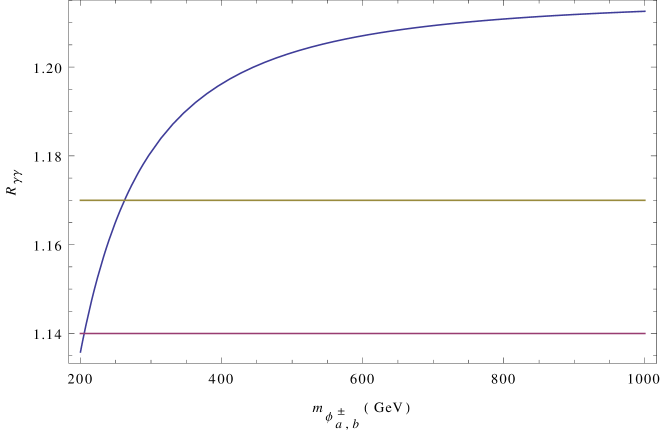
Refer to caption
Figure 4: The ratio Rγγsubscript𝑅𝛾𝛾R_{\gamma\gamma} as a function of the charged Higgs masses mϕs±subscript𝑚superscriptsubscriptitalic-ϕ𝑠plus-or-minusm_{\phi_{s}^{\pm}} (s=a,b𝑠𝑎𝑏s=a,b) for ahtt=1subscript𝑎𝑡𝑡1a_{htt}=1. The horizontal lines are the Rγγsubscript𝑅𝛾𝛾R_{\gamma\gamma} experimental values given by CMS and ATLAS, which are equal to 1.140.23+0.26superscriptsubscript1.140.230.261.14_{-0.23}^{+0.26} and 1.17±0.27plus-or-minus1.170.271.17\pm 0.27, respectively Khachatryan:2014ira ; Aad:2014eha .

V Conclusions

In summary we have presented a 3HDM with LFT, where strongly constrained FCNCs are suppressed by virtue of a residual Z3subscript𝑍3Z_{3} symmetry. A small breaking of the Z3subscript𝑍3Z_{3} symmetry can give rise to LFV Higgs decays, occuring naturally in our model due to SU(2)𝑆𝑈2SU(2) singlet scalars in the scalar potential. Furthermore, a small breaking of the Z3subscript𝑍3Z_{3} symmetry also gives rise to CP violation in neutrino oscillations. We obtain a sizable branching ratio particularly in the flavor violating hμτc𝜇superscript𝜏𝑐h\rightarrow\mu\tau^{c} channel, accounting for the 2.4σ2.4𝜎2.4\,\sigma deviation from the SM as indicated by recent CMS results. This is a consequence of mixing between an SM-like Higgs with a nonstandard neutral scalar that can decay into flavor violating final states. If the extra neutral scalars are light, they can partly cancel Higgs loop contributions to llγ𝑙superscript𝑙𝛾l\rightarrow l^{\prime}\gamma, allowing for large flavor violating Yukawa couplings. We thus also expect large branching fractions for heμ𝑒𝜇h\rightarrow e\mu and heτ𝑒𝜏h\rightarrow e\tau in our model, where the latter will be a decisive measurement for its exclusion. Furthermore, the hγγ𝛾𝛾h\rightarrow\gamma\gamma rate measured by ATLAS and CMS favors charged Higgs boson masses of less than 205 GeV, but the large experimental uncertainties still allow for masses of up to 1 TeV in our model.

Acknowledgments

We thank Gautam Bhattacharyya and Ivo de Medeiros Varzielas for useful discussions. A.E.C.H thanks the TU Dortmund for hospitality and for partially financing his visit. A.E.C.H was partially supported by Fondecyt (Chile), Grant No. 11130115 and by DGIP internal Grant No. 111458. M.D.C. thanks the DAAD for supporting his visit to the TU Dortmund.

Appendix A S4subscript𝑆4S_{4} Symmetry

S4subscript𝑆4S_{4}, the group of permutations of four objects, contains five irreducible representations 𝟏,1,2,3,31superscript123superscript3{\mathbf{1},1^{\prime},2,3,3^{\prime}} obeying the following tensor product rules Ishimori:2010au :

𝟑𝟑=𝟏𝟐𝟑𝟑,𝟑𝟑=𝟏𝟐𝟑𝟑,𝟑𝟑=𝟏𝟐𝟑𝟑,formulae-sequencetensor-product33direct-sum123superscript3formulae-sequencetensor-productsuperscript3superscript3direct-sum123superscript3tensor-product3superscript3direct-sumsuperscript123superscript3\displaystyle\mathbf{3}\otimes\mathbf{3}=\mathbf{1}\oplus\mathbf{2}\oplus\mathbf{3}\oplus\mathbf{3^{\prime}},\qquad\mathbf{3^{\prime}}\otimes\mathbf{3^{\prime}}=\mathbf{1}\oplus\mathbf{2}\oplus\mathbf{3}\oplus\mathbf{3^{\prime}},\qquad\mathbf{3}\otimes\mathbf{3^{\prime}}=\mathbf{1^{\prime}}\oplus\mathbf{2}\oplus\mathbf{3}\oplus\mathbf{3^{\prime}}, (177)
𝟐𝟐=𝟏𝟏𝟐,𝟐𝟑=𝟑𝟑,𝟐𝟑=𝟑𝟑,formulae-sequencetensor-product22direct-sum1superscript12formulae-sequencetensor-product23direct-sum3superscript3tensor-product2superscript3direct-sumsuperscript33\displaystyle\mathbf{2}\otimes\mathbf{2}=\mathbf{1}\oplus\mathbf{1^{\prime}}\oplus\mathbf{2},\qquad\mathbf{2}\otimes\mathbf{3}=\mathbf{3}\oplus\mathbf{3^{\prime}},\qquad\mathbf{2}\otimes\mathbf{3^{\prime}}=\mathbf{3^{\prime}}\oplus\mathbf{3}, (178)
𝟑𝟏=𝟑,𝟑𝟏=𝟑,𝟐𝟏=𝟐.formulae-sequencetensor-product3superscript1superscript3formulae-sequencetensor-productsuperscript3superscript13tensor-product2superscript12\displaystyle\mathbf{3}\otimes\mathbf{1^{\prime}}=\mathbf{3^{\prime}},\qquad\mathbf{3^{\prime}}\otimes\mathbf{1^{\prime}}=\mathbf{3},\qquad\mathbf{2}\otimes\mathbf{1^{\prime}}=\mathbf{2}. (179)

Explicitly, the basis used in this paper corresponds to Ref. Ishimori:2010au and results in

(𝐀)𝟑×(𝐁)𝟑=(𝐀𝐁)𝟏+(𝐀Σ𝐁𝐀Σ𝐁)𝟐+({AyBz}{AzBx}{AxBy})𝟑+([AyBz][AzBx][AxBy])𝟑,subscript𝐀3subscript𝐁3subscript𝐀𝐁1subscript𝐀Σ𝐁𝐀superscriptΣ𝐁2subscriptsubscript𝐴𝑦subscript𝐵𝑧subscript𝐴𝑧subscript𝐵𝑥subscript𝐴𝑥subscript𝐵𝑦3subscriptdelimited-[]subscript𝐴𝑦subscript𝐵𝑧delimited-[]subscript𝐴𝑧subscript𝐵𝑥delimited-[]subscript𝐴𝑥subscript𝐵𝑦superscript3\displaystyle({\mathbf{A}})_{\mathbf{3}}\times({\mathbf{B}})_{\mathbf{3}}=({\mathbf{A}}\cdot{\mathbf{B}})_{\mathbf{1}}+\left(\begin{array}[]{c}{\mathbf{A}}\cdot\Sigma\cdot{\mathbf{B}}\\ {\mathbf{A}}\cdot\Sigma^{*}\cdot{\mathbf{B}}\end{array}\right)_{\mathbf{2}}+\left(\begin{array}[]{c}\{A_{y}B_{z}\}\\ \{A_{z}B_{x}\}\\ \{A_{x}B_{y}\}\end{array}\right)_{\mathbf{3}}+\left(\begin{array}[]{c}\left[A_{y}B_{z}\right]\\ \left[A_{z}B_{x}\right]\\ \left[A_{x}B_{y}\right]\end{array}\right)_{\mathbf{3}^{\prime}}, (188)
(𝐀)𝟑×(𝐁)𝟑=(𝐀𝐁)𝟏+(𝐀Σ𝐁𝐀Σ𝐁)𝟐+({AyBz}{AzBx}{AxBy})𝟑+([AyBz][AzBx][AxBy])𝟑,subscript𝐀superscript3subscript𝐁superscript3subscript𝐀𝐁1subscript𝐀Σ𝐁𝐀superscriptΣ𝐁2subscriptsubscript𝐴𝑦subscript𝐵𝑧subscript𝐴𝑧subscript𝐵𝑥subscript𝐴𝑥subscript𝐵𝑦3subscriptdelimited-[]subscript𝐴𝑦subscript𝐵𝑧delimited-[]subscript𝐴𝑧subscript𝐵𝑥delimited-[]subscript𝐴𝑥subscript𝐵𝑦superscript3\displaystyle({\mathbf{A}})_{\mathbf{3}^{\prime}}\times({\mathbf{B}})_{\mathbf{3}^{\prime}}=({\mathbf{A}}\cdot{\mathbf{B}})_{\mathbf{1}}+\left(\begin{array}[]{c}{\mathbf{A}}\cdot\Sigma\cdot{\mathbf{B}}\\ {\mathbf{A}}\cdot\Sigma^{*}\cdot{\mathbf{B}}\end{array}\right)_{\mathbf{2}}+\left(\begin{array}[]{c}\{A_{y}B_{z}\}\\ \{A_{z}B_{x}\}\\ \{A_{x}B_{y}\}\end{array}\right)_{\mathbf{3}}+\left(\begin{array}[]{c}\left[A_{y}B_{z}\right]\\ \left[A_{z}B_{x}\right]\\ \left[A_{x}B_{y}\right]\end{array}\right)_{\mathbf{3}^{\prime}}, (197)
(𝐀)𝟑×(𝐁)𝟑=(𝐀𝐁)𝟏+(𝐀Σ𝐁𝐀Σ𝐁)𝟐+({AyBz}{AzBx}{AxBy})𝟑+([AyBz][AzBx][AxBy])𝟑,subscript𝐀3subscript𝐁superscript3subscript𝐀𝐁superscript1subscript𝐀Σ𝐁𝐀superscriptΣ𝐁2subscriptsubscript𝐴𝑦subscript𝐵𝑧subscript𝐴𝑧subscript𝐵𝑥subscript𝐴𝑥subscript𝐵𝑦superscript3subscriptdelimited-[]subscript𝐴𝑦subscript𝐵𝑧delimited-[]subscript𝐴𝑧subscript𝐵𝑥delimited-[]subscript𝐴𝑥subscript𝐵𝑦3\displaystyle({\mathbf{A}})_{\mathbf{3}}\times({\mathbf{B}})_{\mathbf{3}^{\prime}}=({\mathbf{A}}\cdot{\mathbf{B}})_{\mathbf{1}^{\prime}}+\left(\begin{array}[]{c}{\mathbf{A}}\cdot\Sigma\cdot{\mathbf{B}}\\ -{\mathbf{A}}\cdot\Sigma^{*}\cdot{\mathbf{B}}\end{array}\right)_{\mathbf{2}}+\left(\begin{array}[]{c}\{A_{y}B_{z}\}\\ \{A_{z}B_{x}\}\\ \{A_{x}B_{y}\}\end{array}\right)_{\mathbf{3}^{\prime}}+\left(\begin{array}[]{c}\left[A_{y}B_{z}\right]\\ \left[A_{z}B_{x}\right]\\ \left[A_{x}B_{y}\right]\end{array}\right)_{\mathbf{3}}, (206)
(𝐀)𝟐×(𝐁)𝟐={AxBy}𝟏+[AxBy]𝟏+(AyByAxBx)𝟐,subscript𝐀2subscript𝐁2subscriptsubscript𝐴𝑥subscript𝐵𝑦1subscriptdelimited-[]subscript𝐴𝑥subscript𝐵𝑦superscript1subscriptsubscript𝐴𝑦subscript𝐵𝑦subscript𝐴𝑥subscript𝐵𝑥2\displaystyle({\mathbf{A}})_{\mathbf{2}}\times({\mathbf{B}})_{\mathbf{2}}=\{A_{x}B_{y}\}_{\mathbf{1}}+\left[A_{x}B_{y}\right]_{\mathbf{1}^{\prime}}+\left(\begin{array}[]{c}A_{y}B_{y}\\ A_{x}B_{x}\end{array}\right)_{\mathbf{2}}, (209)
(AxAy)𝟐×(BxByBz)𝟑=((Ax+Ay)Bx(ω2Ax+ωAy)By(ωAx+ω2Ay)Bz)𝟑+((AxAy)Bx(ω2AxωAy)By(ωAxω2Ay)Bz)𝟑,subscriptsubscript𝐴𝑥subscript𝐴𝑦2subscriptsubscript𝐵𝑥subscript𝐵𝑦subscript𝐵𝑧3subscriptsubscript𝐴𝑥subscript𝐴𝑦subscript𝐵𝑥superscript𝜔2subscript𝐴𝑥𝜔subscript𝐴𝑦subscript𝐵𝑦𝜔subscript𝐴𝑥superscript𝜔2subscript𝐴𝑦subscript𝐵𝑧3subscriptsubscript𝐴𝑥subscript𝐴𝑦subscript𝐵𝑥superscript𝜔2subscript𝐴𝑥𝜔subscript𝐴𝑦subscript𝐵𝑦𝜔subscript𝐴𝑥superscript𝜔2subscript𝐴𝑦subscript𝐵𝑧superscript3\displaystyle\left(\begin{array}[]{c}A_{x}\\ A_{y}\end{array}\right)_{\mathbf{2}}\times\left(\begin{array}[]{c}B_{x}\\ B_{y}\\ B_{z}\end{array}\right)_{\mathbf{3}}=\left(\begin{array}[]{c}(A_{x}+A_{y})B_{x}\\ (\omega^{2}A_{x}+\omega A_{y})B_{y}\\ (\omega A_{x}+\omega^{2}A_{y})B_{z}\end{array}\right)_{\mathbf{3}}+\left(\begin{array}[]{c}(A_{x}-A_{y})B_{x}\\ (\omega^{2}A_{x}-\omega A_{y})B_{y}\\ (\omega A_{x}-\omega^{2}A_{y})B_{z}\end{array}\right)_{{\mathbf{3}}^{\prime}}, (221)
(AxAy)𝟐×(BxByBz)𝟑=((Ax+Ay)Bx(ω2Ax+ωAy)By(ωAx+ω2Ay)Bz)𝟑+((AxAy)Bx(ω2AxωAy)By(ωAxω2Ay)Bz)𝟑,subscriptsubscript𝐴𝑥subscript𝐴𝑦2subscriptsubscript𝐵𝑥subscript𝐵𝑦subscript𝐵𝑧superscript3subscriptsubscript𝐴𝑥subscript𝐴𝑦subscript𝐵𝑥superscript𝜔2subscript𝐴𝑥𝜔subscript𝐴𝑦subscript𝐵𝑦𝜔subscript𝐴𝑥superscript𝜔2subscript𝐴𝑦subscript𝐵𝑧superscript3subscriptsubscript𝐴𝑥subscript𝐴𝑦subscript𝐵𝑥superscript𝜔2subscript𝐴𝑥𝜔subscript𝐴𝑦subscript𝐵𝑦𝜔subscript𝐴𝑥superscript𝜔2subscript𝐴𝑦subscript𝐵𝑧3\displaystyle\left(\begin{array}[]{c}A_{x}\\ A_{y}\end{array}\right)_{\mathbf{2}}\times\left(\begin{array}[]{c}B_{x}\\ B_{y}\\ B_{z}\end{array}\right)_{{\mathbf{3}}^{\prime}}=\left(\begin{array}[]{c}(A_{x}+A_{y})B_{x}\\ (\omega^{2}A_{x}+\omega A_{y})B_{y}\\ (\omega A_{x}+\omega^{2}A_{y})B_{z}\end{array}\right)_{{\mathbf{3}}^{\prime}}+\left(\begin{array}[]{c}(A_{x}-A_{y})B_{x}\\ (\omega^{2}A_{x}-\omega A_{y})B_{y}\\ (\omega A_{x}-\omega^{2}A_{y})B_{z}\end{array}\right)_{\mathbf{3}}, (233)

with

𝐀𝐁𝐀𝐁\displaystyle{\mathbf{A}}\cdot{\mathbf{B}} =AxBx+AyBy+AzBz,absentsubscript𝐴𝑥subscript𝐵𝑥subscript𝐴𝑦subscript𝐵𝑦subscript𝐴𝑧subscript𝐵𝑧\displaystyle=A_{x}B_{x}+A_{y}B_{y}+A_{z}B_{z}, (234)
{AxBy}subscript𝐴𝑥subscript𝐵𝑦\displaystyle\{A_{x}B_{y}\} =AxBy+AyBx,absentsubscript𝐴𝑥subscript𝐵𝑦subscript𝐴𝑦subscript𝐵𝑥\displaystyle=A_{x}B_{y}+A_{y}B_{x}, (235)
[AxBy]delimited-[]subscript𝐴𝑥subscript𝐵𝑦\displaystyle\left[A_{x}B_{y}\right] =AxByAyBx,absentsubscript𝐴𝑥subscript𝐵𝑦subscript𝐴𝑦subscript𝐵𝑥\displaystyle=A_{x}B_{y}-A_{y}B_{x}, (236)
𝐀Σ𝐁𝐀Σ𝐁\displaystyle{\mathbf{A}}\cdot\Sigma\cdot{\mathbf{B}} =AxBx+ωAyBy+ω2AzBz,absentsubscript𝐴𝑥subscript𝐵𝑥𝜔subscript𝐴𝑦subscript𝐵𝑦superscript𝜔2subscript𝐴𝑧subscript𝐵𝑧\displaystyle=A_{x}B_{x}+\omega A_{y}B_{y}+\omega^{2}A_{z}B_{z}, (237)
𝐀Σ𝐁𝐀superscriptΣ𝐁\displaystyle{\mathbf{A}}\cdot\Sigma^{*}\cdot{\mathbf{B}} =AxBx+ω2AyBy+ωAzBz,absentsubscript𝐴𝑥subscript𝐵𝑥superscript𝜔2subscript𝐴𝑦subscript𝐵𝑦𝜔subscript𝐴𝑧subscript𝐵𝑧\displaystyle=A_{x}B_{x}+\omega^{2}A_{y}B_{y}+\omega A_{z}B_{z}, (238)

where ω=e2πi/3𝜔superscript𝑒2𝜋𝑖3\omega=e^{2\pi i/3} is a complex square root of unity.

Appendix B T and S parameter constraints

The inclusion of the extra scalar particles modifies the oblique corrections of the SM, the values which have been extracted from high precision experiments. Consequently, the validity of the different flavor models that we are considering depends on the condition that the extra particles do not contradict those experimental results. These oblique corrections are parametrized in terms of the two well-known quantities T𝑇T and S𝑆S. The T𝑇T parameter is defined as Peskin:1991sw ; Altarelli:1990zd ; Barbieri:2004qk ; Barbieri:2007gi :

T=Π33(0)Π11(0)MW2αem(mZ).𝑇subscriptΠ330subscriptΠ110superscriptsubscript𝑀𝑊2subscript𝛼𝑒𝑚subscript𝑚𝑍T=\frac{\Pi_{33}\left(0\right)-\Pi_{11}\left(0\right)}{M_{W}^{2}\ \alpha_{em}\left(m_{Z}\right)}. (239)

where Π11(0)subscriptΠ110\Pi_{11}\left(0\right) and Π33(0)subscriptΠ330\Pi_{33}\left(0\right) are the vacuum polarization amplitudes at q2=0superscript𝑞20q^{2}=0 for loop diagrams having gauge bosons Wμ1superscriptsubscript𝑊𝜇1W_{\mu}^{1}, Wμ1superscriptsubscript𝑊𝜇1W_{\mu}^{1} and Wμ3superscriptsubscript𝑊𝜇3W_{\mu}^{3}, Wμ3superscriptsubscript𝑊𝜇3W_{\mu}^{3} in the external lines, respectively.

In turn, the S𝑆S parameter is defined by Peskin:1991sw ; Altarelli:1990zd ; Barbieri:2004qk ; Barbieri:2007gi :

S=4sin2θWαem(mZ)ggdΠ30(q2)dq2|q2=0,S=\frac{4\sin^{2}\theta_{W}}{\alpha_{em}\left(m_{Z}\right)}\frac{g}{g^{\prime}}\frac{d\Pi_{30}\left(q^{2}\right)}{dq^{2}}\biggl{|}_{q^{2}=0}, (240)

where Π30(q2)subscriptΠ30superscript𝑞2\Pi_{30}\left(q^{2}\right) is the vacuum polarization amplitude for a loop diagram having Wμ3superscriptsubscript𝑊𝜇3W_{\mu}^{3} and Bμsubscript𝐵𝜇B_{\mu} in the external lines.

The Feynman diagrams contributing to the T𝑇T and S𝑆S parameters are shown in Figs. 5 and 6.

Refer to caption
Figure 5: One-loop Feynman diagrams contributing to the T𝑇T parameter.
Refer to caption
Figure 6: One-loop Feynman diagrams contributing to the S𝑆S parameter.

We can split the T𝑇T and S𝑆S parameters as T=TSM+ΔT𝑇subscript𝑇𝑆𝑀Δ𝑇T=T_{SM}+\Delta T and S=SSM+ΔS𝑆subscript𝑆𝑆𝑀Δ𝑆S=S_{SM}+\Delta S, where TSMsubscript𝑇𝑆𝑀T_{SM} and SSMsubscript𝑆𝑆𝑀S_{SM} are the contributions from the SM, while ΔTΔ𝑇\Delta T and ΔSΔ𝑆\Delta S contain all the contributions involving the extra particles

TSM=316πcos2θWln(mh2mW2),SSM=112πln(mh2mW2)formulae-sequencesubscript𝑇𝑆𝑀316𝜋superscript2subscript𝜃𝑊superscriptsubscript𝑚2superscriptsubscript𝑚𝑊2subscript𝑆𝑆𝑀112𝜋superscriptsubscript𝑚2superscriptsubscript𝑚𝑊2T_{SM}=-\frac{3}{16\pi\cos^{2}\theta_{W}}\ln\left(\frac{m_{h}^{2}}{m_{W}^{2}}\right),\hskip 5.69046pt\hskip 5.69046pt\hskip 5.69046pt\hskip 5.69046pt\hskip 5.69046pt\hskip 5.69046pt\hskip 5.69046ptS_{SM}=\frac{1}{12\pi}\ln\left(\frac{m_{h}^{2}}{m_{W}^{2}}\right) (241)
ΔT116π2v2αem(mZ)f=a,b[mmϕf±22H(mϕfI02,mϕf±2)+H(mϕfR02,mϕfI02)H(mϕfR02,mϕf±2)]similar-to-or-equalsΔ𝑇116superscript𝜋2superscript𝑣2subscript𝛼𝑒𝑚subscript𝑚𝑍subscript𝑓𝑎𝑏delimited-[]superscriptsubscript𝑚superscriptsubscript𝑚superscriptsubscriptitalic-ϕ𝑓plus-or-minus22𝐻superscriptsubscript𝑚superscriptsubscriptitalic-ϕ𝑓𝐼02superscriptsubscript𝑚superscriptsubscriptitalic-ϕ𝑓plus-or-minus2𝐻superscriptsubscript𝑚superscriptsubscriptitalic-ϕ𝑓𝑅02superscriptsubscript𝑚superscriptsubscriptitalic-ϕ𝑓𝐼02𝐻superscriptsubscript𝑚superscriptsubscriptitalic-ϕ𝑓𝑅02superscriptsubscript𝑚superscriptsubscriptitalic-ϕ𝑓plus-or-minus2\Delta T\simeq\frac{1}{16\pi^{2}v^{2}\alpha_{em}\left(m_{Z}\right)}\sum_{f=a,b}\left[m_{m_{\phi_{f}^{\pm}}^{2}}^{2}-H\left(m_{\phi_{fI}^{0}}^{2},m_{\phi_{f}^{\pm}}^{2}\right)+H\left(m_{\phi_{fR}^{0}}^{2},m_{\phi_{fI}^{0}}^{2}\right)-H\left(m_{\phi_{fR}^{0}}^{2},m_{\phi_{f}^{\pm}}^{2}\right)\right] (242)
ΔS112πf=a,bK(mϕfR02,mϕfI02,mϕf±2),similar-to-or-equalsΔ𝑆112𝜋subscript𝑓𝑎𝑏𝐾superscriptsubscript𝑚superscriptsubscriptitalic-ϕ𝑓𝑅02superscriptsubscript𝑚superscriptsubscriptitalic-ϕ𝑓𝐼02superscriptsubscript𝑚superscriptsubscriptitalic-ϕ𝑓plus-or-minus2\Delta S\simeq\frac{1}{12\pi}\sum_{f=a,b}K\left(m_{\phi_{fR}^{0}}^{2},m_{\phi_{fI}^{0}}^{2},m_{\phi_{f}^{\pm}}^{2}\right), (243)

where we introduced the following functions Hernandez:2015rfa :

H(m12,m22)=m12m22m12m22ln(m12m22),limm2m1H(m12,m22)=m12.formulae-sequence𝐻superscriptsubscript𝑚12superscriptsubscript𝑚22superscriptsubscript𝑚12superscriptsubscript𝑚22superscriptsubscript𝑚12superscriptsubscript𝑚22superscriptsubscript𝑚12superscriptsubscript𝑚22subscriptsubscript𝑚2subscript𝑚1𝐻superscriptsubscript𝑚12superscriptsubscript𝑚22superscriptsubscript𝑚12H\left(m_{1}^{2},m_{2}^{2}\right)=\frac{m_{1}^{2}m_{2}^{2}}{m_{1}^{2}-m_{2}^{2}}\ln\left(\frac{m_{1}^{2}}{m_{2}^{2}}\right),\hskip 42.67912pt\hskip 42.67912pt\lim_{m_{2}\rightarrow m_{1}}H\left(m_{1}^{2},m_{2}^{2}\right)=m_{1}^{2}. (244)
K(m12,m22,m32)𝐾superscriptsubscript𝑚12superscriptsubscript𝑚22superscriptsubscript𝑚32\displaystyle K\left(m_{1}^{2},m_{2}^{2},m_{3}^{2}\right) =\displaystyle= 1(m22m12)3{m14(3m22m12)ln(m12m32)m24(3m12m22)ln(m22m32)\displaystyle\frac{1}{\left(m_{2}^{2}-m_{1}^{2}\right){}^{3}}\left\{m_{1}^{4}\left(3m_{2}^{2}-m_{1}^{2}\right)\ln\left(\frac{m_{1}^{2}}{m_{3}^{2}}\right)-m_{2}^{4}\left(3m_{1}^{2}-m_{2}^{2}\right)\ln\left(\frac{m_{2}^{2}}{m_{3}^{2}}\right)\right. (245)
16[27m12m22(m12m22)+5(m26m16)]}.\displaystyle-\left.\frac{1}{6}\left[27m_{1}^{2}m_{2}^{2}\left(m_{1}^{2}-m_{2}^{2}\right)+5\left(m_{2}^{6}-m_{1}^{6}\right)\right]\right\}.

The experimental results on T𝑇T and S𝑆S restrict ΔTΔ𝑇\Delta T and ΔSΔ𝑆\Delta S to lie inside a region in the ΔSΔTΔ𝑆Δ𝑇\Delta S-\Delta T plane. At the 95%percent9595\% C.L. (confidence level), these regions are the elliptic contours shown in Fig. 7. The origin ΔS=ΔT=0Δ𝑆Δ𝑇0\Delta S=\Delta T=0 corresponds to the SM value, with mh=125.5subscript𝑚125.5m_{h}=125.5 GeV and mt=176subscript𝑚𝑡176m_{t}=176 GeV. One can consider a scenario in which the heavy neutral CP-even and neutral CP-odd scalars are degenerate. For a mass of mϕ(a,b)I0=mϕ(a,b)R0=130subscript𝑚superscriptsubscriptitalic-ϕ𝑎𝑏𝐼0subscript𝑚superscriptsubscriptitalic-ϕ𝑎𝑏𝑅0130m_{\phi_{(a,b)I}^{0}}=m_{\phi_{(a,b)R}^{0}}=130 GeV, consistency with the T𝑇T and S𝑆S parameters confines the masses of the charged scalars to 130130130 GeV mϕ(a,b)±absentsubscript𝑚superscriptsubscriptitalic-ϕ𝑎𝑏plus-or-minusabsent\leq m_{\phi_{(a,b)}^{\pm}}\leq 196196196 GeV, whereas for mϕ(a,b)I0=mϕ(a,b)R0=600subscript𝑚superscriptsubscriptitalic-ϕ𝑎𝑏𝐼0subscript𝑚superscriptsubscriptitalic-ϕ𝑎𝑏𝑅0600m_{\phi_{(a,b)I}^{0}}=m_{\phi_{(a,b)R}^{0}}=600 GeV, the charged scalar masses are in the range 600600600 GeV mϕ(a,b)±absentsubscript𝑚superscriptsubscriptitalic-ϕ𝑎𝑏plus-or-minusabsent\leq m_{\phi_{(a,b)}^{\pm}}\leq 672672672 GeV while for mϕ(a,b)I0=mϕ(a,b)R0=1subscript𝑚superscriptsubscriptitalic-ϕ𝑎𝑏𝐼0subscript𝑚superscriptsubscriptitalic-ϕ𝑎𝑏𝑅01m_{\phi_{(a,b)I}^{0}}=m_{\phi_{(a,b)R}^{0}}=1 TeV, the masses of the charged scalars range between 925 and 990 GeV. In Figs. 7(a)-7(c) we show the allowed regions for the ΔTΔ𝑇\Delta T and ΔSΔ𝑆\Delta S parameters, for the three sets of values of mϕ(a,b)I0subscript𝑚superscriptsubscriptitalic-ϕ𝑎𝑏𝐼0m_{\phi_{(a,b)I}^{0}} and mϕ(a,b)R0subscript𝑚superscriptsubscriptitalic-ϕ𝑎𝑏𝑅0m_{\phi_{(a,b)R}^{0}} previously indicated. The line going upwards inside the ellipses corresponds to the several (ΔS,ΔT)Δ𝑆Δ𝑇(\Delta S,\Delta T) points of the model when the charged scalar masses are varied inside the interval previously specified.

Refer to caption
(a)  mϕ(a,b)I0=mϕ(a,b)R0=130subscript𝑚superscriptsubscriptitalic-ϕ𝑎𝑏𝐼0subscript𝑚superscriptsubscriptitalic-ϕ𝑎𝑏𝑅0130m_{\phi_{(a,b)I}^{0}}=m_{\phi_{(a,b)R}^{0}}=130 GeV
Refer to caption
(b)  mϕ(a,b)I0=mϕ(a,b)R0=600subscript𝑚superscriptsubscriptitalic-ϕ𝑎𝑏𝐼0subscript𝑚superscriptsubscriptitalic-ϕ𝑎𝑏𝑅0600m_{\phi_{(a,b)I}^{0}}=m_{\phi_{(a,b)R}^{0}}=600 GeV
Refer to caption
(c)  mϕ(a,b)I0=mϕ(a,b)R0=1subscript𝑚superscriptsubscriptitalic-ϕ𝑎𝑏𝐼0subscript𝑚superscriptsubscriptitalic-ϕ𝑎𝑏𝑅01m_{\phi_{(a,b)I}^{0}}=m_{\phi_{(a,b)R}^{0}}=1 TeV

(7.a)                                               (7.b)                                               (7.c)

Figure 7: The ΔSΔTΔ𝑆Δ𝑇\Delta S-\Delta T plane, where the ellipses denote the experimentally allowed region at 95%percent9595\% C.L. taken from Baak:2013ppa ; Baak:2012kk ; Baak:2011ze . The origin ΔS=ΔT=0Δ𝑆Δ𝑇0\Delta S=\Delta T=0 corresponds to the SM value, with mh=125.5subscript𝑚125.5m_{h}=125.5 GeV and mt=176subscript𝑚𝑡176m_{t}=176 GeV. Figures (a), (b) and (c) correspond to two different sets of values for the masses of the neutral non-SM Higgs bosons, as indicated. The mass mϕ(a,b)±subscript𝑚superscriptsubscriptitalic-ϕ𝑎𝑏plus-or-minusm_{\phi_{(a,b)}^{\pm}} of the charged Higgs bosons varies between 130130130 GeV mϕ(a,b)±absentsubscript𝑚superscriptsubscriptitalic-ϕ𝑎𝑏plus-or-minusabsent\leq m_{\phi_{(a,b)}^{\pm}}\leq 196196196 GeV (Fig. 7(a), 600600600 GeV mϕ(a,b)±absentsubscript𝑚superscriptsubscriptitalic-ϕ𝑎𝑏plus-or-minusabsent\leq m_{\phi_{(a,b)}^{\pm}}\leq 672672672 GeV ( Fig. 7(b), 925925925 GeV mϕ(a,b)±absentsubscript𝑚superscriptsubscriptitalic-ϕ𝑎𝑏plus-or-minusabsent\leq m_{\phi_{(a,b)}^{\pm}}\leq 990990990 GeV (Fig. 7(c). The lines originating in the center of the plot and running up towards the ellipses correspond to the obtained values of the ΔTΔ𝑇\Delta T and ΔSΔ𝑆\Delta S parameters in our model, as the charged Higgs boson masses are varied in the aforementioned ranges.

Appendix C Quark masses and mixings

The relevant S4Z2′′Z6Z12tensor-productsubscript𝑆4superscriptsubscript𝑍2′′subscript𝑍6subscript𝑍12S_{4}\otimes Z_{2}^{\prime\prime}\otimes Z_{6}\otimes Z_{12} -invariant Yukawa terms for the up-type quark sector are

(U)superscript𝑈\displaystyle\mathcal{L}^{\left(U\right)} =\displaystyle= y1(t)[Qϕ]3tRρΛ+y2(t)ΛQ[ϕρ]3tR+y3(t)[Qϕ]3tRρΛ+y4(t)ΛQ[ϕρ]3tRsuperscriptsubscript𝑦1𝑡subscriptdelimited-[]𝑄italic-ϕsuperscript3subscript𝑡𝑅𝜌Λsuperscriptsubscript𝑦2𝑡Λ𝑄subscriptdelimited-[]italic-ϕ𝜌superscript3subscript𝑡𝑅superscriptsubscript𝑦3𝑡subscriptdelimited-[]𝑄italic-ϕsuperscript3subscript𝑡𝑅𝜌Λsuperscriptsubscript𝑦4𝑡Λ𝑄subscriptdelimited-[]italic-ϕ𝜌superscript3subscript𝑡𝑅\displaystyle y_{1}^{\left(t\right)}\left[Q\phi\right]_{3^{\prime}}t_{R}\frac{\rho}{\Lambda}+\frac{y_{2}^{\left(t\right)}}{\Lambda}Q\left[\phi\rho\right]_{3^{\prime}}t_{R}+y_{3}^{\left(t\right)}\left[Q\phi\right]_{3^{\prime}}t_{R}\frac{\rho}{\Lambda}+\frac{y_{4}^{\left(t\right)}}{\Lambda}Q\left[\phi\rho\right]_{3^{\prime}}t_{R} (246)
+x1(t)[Qϕ]3tRφΛ+x2(t)ΛQ[ϕφ]3tR+x3(t)[Qϕ]3tRφΛ+x4(t)ΛQ[ϕφ]3tRsuperscriptsubscript𝑥1𝑡subscriptdelimited-[]𝑄italic-ϕ3subscript𝑡𝑅𝜑Λsuperscriptsubscript𝑥2𝑡Λ𝑄subscriptdelimited-[]italic-ϕ𝜑superscript3subscript𝑡𝑅superscriptsubscript𝑥3𝑡subscriptdelimited-[]𝑄italic-ϕ3subscript𝑡𝑅𝜑Λsuperscriptsubscript𝑥4𝑡Λ𝑄subscriptdelimited-[]italic-ϕ𝜑superscript3subscript𝑡𝑅\displaystyle+x_{1}^{\left(t\right)}\left[Q\phi\right]_{3}t_{R}\frac{\varphi}{\Lambda}+\frac{x_{2}^{\left(t\right)}}{\Lambda}Q\left[\phi\varphi\right]_{3^{\prime}}t_{R}+x_{3}^{\left(t\right)}\left[Q\phi\right]_{3}t_{R}\frac{\varphi}{\Lambda}+\frac{x_{4}^{\left(t\right)}}{\Lambda}Q\left[\phi\varphi\right]_{3^{\prime}}t_{R}
+y1(c)[Qϕ]3cRρΛ+y2(c)ΛQ[ϕρ]3cR+y3(c)[Qϕ]3cRρΛ+y4(c)ΛQ[ϕρ]3cRsuperscriptsubscript𝑦1𝑐subscriptdelimited-[]𝑄italic-ϕsuperscript3subscript𝑐𝑅𝜌Λsuperscriptsubscript𝑦2𝑐Λ𝑄subscriptdelimited-[]italic-ϕ𝜌superscript3subscript𝑐𝑅superscriptsubscript𝑦3𝑐subscriptdelimited-[]𝑄italic-ϕsuperscript3subscript𝑐𝑅𝜌Λsuperscriptsubscript𝑦4𝑐Λ𝑄subscriptdelimited-[]italic-ϕ𝜌superscript3subscript𝑐𝑅\displaystyle+y_{1}^{\left(c\right)}\left[Q\phi\right]_{3^{\prime}}c_{R}\frac{\rho}{\Lambda}+\frac{y_{2}^{\left(c\right)}}{\Lambda}Q\left[\phi\rho\right]_{3^{\prime}}c_{R}+y_{3}^{\left(c\right)}\left[Q\phi\right]_{3^{\prime}}c_{R}\frac{\rho}{\Lambda}+\frac{y_{4}^{\left(c\right)}}{\Lambda}Q\left[\phi\rho\right]_{3^{\prime}}c_{R}
+x1(c)[Qϕ]3cRφΛ+x2(c)ΛQ[ϕφ]3cR+x3(c)[Qϕ]3cRφΛ+x4(c)ΛQ[ϕφ]3cR+x0(u)[Qϕ]1uRΩ23Λ3superscriptsubscript𝑥1𝑐subscriptdelimited-[]𝑄italic-ϕ3subscript𝑐𝑅𝜑Λsuperscriptsubscript𝑥2𝑐Λ𝑄subscriptdelimited-[]italic-ϕ𝜑superscript3subscript𝑐𝑅superscriptsubscript𝑥3𝑐subscriptdelimited-[]𝑄italic-ϕ3subscript𝑐𝑅𝜑Λsuperscriptsubscript𝑥4𝑐Λ𝑄subscriptdelimited-[]italic-ϕ𝜑superscript3subscript𝑐𝑅superscriptsubscript𝑥0𝑢subscriptdelimited-[]𝑄italic-ϕ1subscript𝑢𝑅superscriptsubscriptΩ23superscriptΛ3\displaystyle+x_{1}^{\left(c\right)}\left[Q\phi\right]_{3}c_{R}\frac{\varphi}{\Lambda}+\frac{x_{2}^{\left(c\right)}}{\Lambda}Q\left[\phi\varphi\right]_{3^{\prime}}c_{R}+x_{3}^{\left(c\right)}\left[Q\phi\right]_{3}c_{R}\frac{\varphi}{\Lambda}+\frac{x_{4}^{\left(c\right)}}{\Lambda}Q\left[\phi\varphi\right]_{3^{\prime}}c_{R}+x_{0}^{\left(u\right)}\left[Q\phi\right]_{1}u_{R}\frac{\Omega_{2}^{3}}{\Lambda^{3}}
+y1(u)[Qϕ]3uRρΩ12Λ3+y2(u)Q[ϕρ]3uRΩ12Λ3+y3(u)[Qϕ]3uRρΩ12Λ4+y4(u)ΛQ[ϕρ]3uRΩ12Λ3superscriptsubscript𝑦1𝑢subscriptdelimited-[]𝑄italic-ϕsuperscript3subscript𝑢𝑅𝜌superscriptsubscriptΩ12superscriptΛ3superscriptsubscript𝑦2𝑢𝑄subscriptdelimited-[]italic-ϕ𝜌superscript3subscript𝑢𝑅superscriptsubscriptΩ12superscriptΛ3superscriptsubscript𝑦3𝑢subscriptdelimited-[]𝑄italic-ϕsuperscript3subscript𝑢𝑅𝜌superscriptsubscriptΩ12superscriptΛ4superscriptsubscript𝑦4𝑢Λ𝑄subscriptdelimited-[]italic-ϕ𝜌superscript3subscript𝑢𝑅superscriptsubscriptΩ12superscriptΛ3\displaystyle+y_{1}^{\left(u\right)}\left[Q\phi\right]_{3^{\prime}}u_{R}\frac{\rho\Omega_{1}^{2}}{\Lambda^{3}}+y_{2}^{\left(u\right)}Q\left[\phi\rho\right]_{3^{\prime}}u_{R}\frac{\Omega_{1}^{2}}{\Lambda^{3}}+y_{3}^{\left(u\right)}\left[Q\phi\right]_{3^{\prime}}u_{R}\frac{\rho\Omega_{1}^{2}}{\Lambda^{4}}+\frac{y_{4}^{\left(u\right)}}{\Lambda}Q\left[\phi\rho\right]_{3^{\prime}}u_{R}\frac{\Omega_{1}^{2}}{\Lambda^{3}}
+x1(u)[Qϕ]3uRφΩ12Λ3+x2(u)Q[ϕφ]3uRΩ12Λ3+x3(c)[Qϕ]3uRφΛ+x4(c)ΛQ[ϕφ]3uRΩ12Λ3superscriptsubscript𝑥1𝑢subscriptdelimited-[]𝑄italic-ϕsuperscript3subscript𝑢𝑅𝜑superscriptsubscriptΩ12superscriptΛ3superscriptsubscript𝑥2𝑢𝑄subscriptdelimited-[]italic-ϕ𝜑superscript3subscript𝑢𝑅superscriptsubscriptΩ12superscriptΛ3superscriptsubscript𝑥3𝑐subscriptdelimited-[]𝑄italic-ϕ3subscript𝑢𝑅𝜑Λsuperscriptsubscript𝑥4𝑐Λ𝑄subscriptdelimited-[]italic-ϕ𝜑superscript3subscript𝑢𝑅superscriptsubscriptΩ12superscriptΛ3\displaystyle+x_{1}^{\left(u\right)}\left[Q\phi\right]_{3^{\prime}}u_{R}\frac{\varphi\Omega_{1}^{2}}{\Lambda^{3}}+x_{2}^{\left(u\right)}Q\left[\phi\varphi\right]_{3^{\prime}}u_{R}\frac{\Omega_{1}^{2}}{\Lambda^{3}}+x_{3}^{\left(c\right)}\left[Q\phi\right]_{3}u_{R}\frac{\varphi}{\Lambda}+\frac{x_{4}^{\left(c\right)}}{\Lambda}Q\left[\phi\varphi\right]_{3^{\prime}}u_{R}\frac{\Omega_{1}^{2}}{\Lambda^{3}}

and for the down-type quarks

1(D)superscriptsubscript1𝐷\displaystyle\mathcal{L}_{1}^{\left(D\right)} =\displaystyle= y1(b)[Qϕ]3bRρΩ33Λ4+y2(b)ΛQ[ϕρ]3bRΩ33Λ3+y3(b)[Qϕ]3bRρΩ33Λ4+y4(b)ΛQ[ϕρ]3bRΩ33Λ3superscriptsubscript𝑦1𝑏subscriptdelimited-[]𝑄italic-ϕsuperscript3subscript𝑏𝑅𝜌superscriptsubscriptΩ33superscriptΛ4superscriptsubscript𝑦2𝑏Λ𝑄subscriptdelimited-[]italic-ϕ𝜌superscript3subscript𝑏𝑅superscriptsubscriptΩ33superscriptΛ3superscriptsubscript𝑦3𝑏subscriptdelimited-[]𝑄italic-ϕsuperscript3subscript𝑏𝑅𝜌superscriptsubscriptΩ33superscriptΛ4superscriptsubscript𝑦4𝑏Λ𝑄subscriptdelimited-[]italic-ϕ𝜌superscript3subscript𝑏𝑅superscriptsubscriptΩ33superscriptΛ3\displaystyle y_{1}^{\left(b\right)}\left[Q\phi\right]_{3^{\prime}}b_{R}\frac{\rho\Omega_{3}^{3}}{\Lambda^{4}}+\frac{y_{2}^{\left(b\right)}}{\Lambda}Q\left[\phi\rho\right]_{3^{\prime}}b_{R}\frac{\Omega_{3}^{3}}{\Lambda^{3}}+y_{3}^{\left(b\right)}\left[Q\phi\right]_{3^{\prime}}b_{R}\frac{\rho\Omega_{3}^{3}}{\Lambda^{4}}+\frac{y_{4}^{\left(b\right)}}{\Lambda}Q\left[\phi\rho\right]_{3^{\prime}}b_{R}\frac{\Omega_{3}^{3}}{\Lambda^{3}}
+x1(b)[Qϕ]3bRφΩ33Λ4+x2(b)ΛQ[ϕφ]3bRΩ33Λ3+x3(b)[Qϕ]3bRφΩ33Λ4+x4(b)ΛQ[ϕφ]3bRΩ33Λ3superscriptsubscript𝑥1𝑏subscriptdelimited-[]𝑄italic-ϕ3subscript𝑏𝑅𝜑superscriptsubscriptΩ33superscriptΛ4superscriptsubscript𝑥2𝑏Λ𝑄subscriptdelimited-[]italic-ϕ𝜑superscript3subscript𝑏𝑅superscriptsubscriptΩ33superscriptΛ3superscriptsubscript𝑥3𝑏subscriptdelimited-[]𝑄italic-ϕ3subscript𝑏𝑅𝜑superscriptsubscriptΩ33superscriptΛ4superscriptsubscript𝑥4𝑏Λ𝑄subscriptdelimited-[]italic-ϕ𝜑superscript3subscript𝑏𝑅superscriptsubscriptΩ33superscriptΛ3\displaystyle+x_{1}^{\left(b\right)}\left[Q\phi\right]_{3}b_{R}\frac{\varphi\Omega_{3}^{3}}{\Lambda^{4}}+\frac{x_{2}^{\left(b\right)}}{\Lambda}Q\left[\phi\varphi\right]_{3^{\prime}}b_{R}\frac{\Omega_{3}^{3}}{\Lambda^{3}}+x_{3}^{\left(b\right)}\left[Q\phi\right]_{3}b_{R}\frac{\varphi\Omega_{3}^{3}}{\Lambda^{4}}+\frac{x_{4}^{\left(b\right)}}{\Lambda}Q\left[\phi\varphi\right]_{3^{\prime}}b_{R}\frac{\Omega_{3}^{3}}{\Lambda^{3}}
+y1(s)[Qϕ]3sRρΩ33Λ4+y2(b)ΛQ[ϕρ]3sRΩ33Λ3+y3(b)[Qϕ]3sRρΩ33Λ4+y4(b)ΛQ[ϕρ]3sRΩ33Λ3superscriptsubscript𝑦1𝑠subscriptdelimited-[]𝑄italic-ϕsuperscript3subscript𝑠𝑅𝜌superscriptsubscriptΩ33superscriptΛ4superscriptsubscript𝑦2𝑏Λ𝑄subscriptdelimited-[]italic-ϕ𝜌superscript3subscript𝑠𝑅superscriptsubscriptΩ33superscriptΛ3superscriptsubscript𝑦3𝑏subscriptdelimited-[]𝑄italic-ϕsuperscript3subscript𝑠𝑅𝜌superscriptsubscriptΩ33superscriptΛ4superscriptsubscript𝑦4𝑏Λ𝑄subscriptdelimited-[]italic-ϕ𝜌superscript3subscript𝑠𝑅superscriptsubscriptΩ33superscriptΛ3\displaystyle+y_{1}^{\left(s\right)}\left[Q\phi\right]_{3^{\prime}}s_{R}\frac{\rho\Omega_{3}^{3}}{\Lambda^{4}}+\frac{y_{2}^{\left(b\right)}}{\Lambda}Q\left[\phi\rho\right]_{3^{\prime}}s_{R}\frac{\Omega_{3}^{3}}{\Lambda^{3}}+y_{3}^{\left(b\right)}\left[Q\phi\right]_{3^{\prime}}s_{R}\frac{\rho\Omega_{3}^{3}}{\Lambda^{4}}+\frac{y_{4}^{\left(b\right)}}{\Lambda}Q\left[\phi\rho\right]_{3^{\prime}}s_{R}\frac{\Omega_{3}^{3}}{\Lambda^{3}}
+x1(s)[Qϕ]3sRφΩ33Λ4+x2(s)ΛQ[ϕφ]3sRΩ33Λ3+x3(s)[Qϕ]3sRφΩ33Λ4+x4(s)ΛQ[ϕφ]3sRΩ33Λ3superscriptsubscript𝑥1𝑠subscriptdelimited-[]𝑄italic-ϕ3subscript𝑠𝑅𝜑superscriptsubscriptΩ33superscriptΛ4superscriptsubscript𝑥2𝑠Λ𝑄subscriptdelimited-[]italic-ϕ𝜑superscript3subscript𝑠𝑅superscriptsubscriptΩ33superscriptΛ3superscriptsubscript𝑥3𝑠subscriptdelimited-[]𝑄italic-ϕ3subscript𝑠𝑅𝜑superscriptsubscriptΩ33superscriptΛ4superscriptsubscript𝑥4𝑠Λ𝑄subscriptdelimited-[]italic-ϕ𝜑superscript3subscript𝑠𝑅superscriptsubscriptΩ33superscriptΛ3\displaystyle+x_{1}^{\left(s\right)}\left[Q\phi\right]_{3}s_{R}\frac{\varphi\Omega_{3}^{3}}{\Lambda^{4}}+\frac{x_{2}^{\left(s\right)}}{\Lambda}Q\left[\phi\varphi\right]_{3^{\prime}}s_{R}\frac{\Omega_{3}^{3}}{\Lambda^{3}}+x_{3}^{\left(s\right)}\left[Q\phi\right]_{3}s_{R}\frac{\varphi\Omega_{3}^{3}}{\Lambda^{4}}+\frac{x_{4}^{\left(s\right)}}{\Lambda}Q\left[\phi\varphi\right]_{3^{\prime}}s_{R}\frac{\Omega_{3}^{3}}{\Lambda^{3}}
+x0(d)[Qϕ]1dRΩ22Ω33Λ5+y1(d)[Qϕ]3dRρΩ1Ω33Λ5+y2(d)Q[ϕρ]3dRΩ1Ω33Λ5+y3(d)[Qϕ]3dRρΩ1Ω33Λ5superscriptsubscript𝑥0𝑑subscriptdelimited-[]𝑄italic-ϕ1subscript𝑑𝑅superscriptsubscriptΩ22superscriptsubscriptΩ33superscriptΛ5superscriptsubscript𝑦1𝑑subscriptdelimited-[]𝑄italic-ϕsuperscript3subscript𝑑𝑅𝜌subscriptΩ1superscriptsubscriptΩ33superscriptΛ5superscriptsubscript𝑦2𝑑𝑄subscriptdelimited-[]italic-ϕ𝜌superscript3subscript𝑑𝑅subscriptΩ1superscriptsubscriptΩ33superscriptΛ5superscriptsubscript𝑦3𝑑subscriptdelimited-[]𝑄italic-ϕsuperscript3subscript𝑑𝑅𝜌subscriptΩ1superscriptsubscriptΩ33superscriptΛ5\displaystyle+x_{0}^{\left(d\right)}\left[Q\phi\right]_{1}d_{R}\frac{\Omega_{2}^{2}\Omega_{3}^{3}}{\Lambda^{5}}+y_{1}^{\left(d\right)}\left[Q\phi\right]_{3^{\prime}}d_{R}\frac{\rho\Omega_{1}\Omega_{3}^{3}}{\Lambda^{5}}+y_{2}^{\left(d\right)}Q\left[\phi\rho\right]_{3^{\prime}}d_{R}\frac{\Omega_{1}\Omega_{3}^{3}}{\Lambda^{5}}+y_{3}^{\left(d\right)}\left[Q\phi\right]_{3^{\prime}}d_{R}\frac{\rho\Omega_{1}\Omega_{3}^{3}}{\Lambda^{5}}
+y4(d)ΛQ[ϕρ]3dRΩ1Ω33Λ5+x1(d)[Qϕ]3dRφΩ1Ω33Λ5+x2(d)Q[ϕφ]3dRΩ1Ω33Λ5superscriptsubscript𝑦4𝑑Λ𝑄subscriptdelimited-[]italic-ϕ𝜌superscript3subscript𝑑𝑅subscriptΩ1superscriptsubscriptΩ33superscriptΛ5superscriptsubscript𝑥1𝑑subscriptdelimited-[]𝑄italic-ϕsuperscript3subscript𝑑𝑅𝜑subscriptΩ1superscriptsubscriptΩ33superscriptΛ5superscriptsubscript𝑥2𝑑𝑄subscriptdelimited-[]italic-ϕ𝜑superscript3subscript𝑑𝑅subscriptΩ1superscriptsubscriptΩ33superscriptΛ5\displaystyle+\frac{y_{4}^{\left(d\right)}}{\Lambda}Q\left[\phi\rho\right]_{3^{\prime}}d_{R}\frac{\Omega_{1}\Omega_{3}^{3}}{\Lambda^{5}}+x_{1}^{\left(d\right)}\left[Q\phi\right]_{3^{\prime}}d_{R}\frac{\varphi\Omega_{1}\Omega_{3}^{3}}{\Lambda^{5}}+x_{2}^{\left(d\right)}Q\left[\phi\varphi\right]_{3^{\prime}}d_{R}\frac{\Omega_{1}\Omega_{3}^{3}}{\Lambda^{5}}
+x3(d)[Qϕ]3dRφΩ33Λ5+x4(d)Q[ϕφ]3dRΩ1Ω33Λ5.superscriptsubscript𝑥3𝑑subscriptdelimited-[]𝑄italic-ϕ3subscript𝑑𝑅𝜑superscriptsubscriptΩ33superscriptΛ5superscriptsubscript𝑥4𝑑𝑄subscriptdelimited-[]italic-ϕ𝜑superscript3subscript𝑑𝑅subscriptΩ1superscriptsubscriptΩ33superscriptΛ5\displaystyle+x_{3}^{\left(d\right)}\left[Q\phi\right]_{3}d_{R}\frac{\varphi\Omega_{3}^{3}}{\Lambda^{5}}+x_{4}^{\left(d\right)}Q\left[\phi\varphi\right]_{3^{\prime}}d_{R}\frac{\Omega_{1}\Omega_{3}^{3}}{\Lambda^{5}}.

Appendix D PMNS matrix after Z3subscript𝑍3Z_{3} breaking

The PMNS matrix receives corrections caused by the perturbation of the VEV alignment. These are approximately given by

U𝑈\displaystyle U similar-to-or-equals\displaystyle\simeq (cosψ3eiϕ2iπ3sinψ3e2iπ33e2iπ3cosψ3+eiϕsinψ3cosψ3eiϕ+2iπ3sinψ3e2iπ33e2iπ3cosψ3+eiϕsinψ3cosψ3eiϕsinψ313cosψ3+eiϕsinψ3)𝜓3superscript𝑒𝑖italic-ϕ2𝑖𝜋3𝜓3superscript𝑒2𝑖𝜋33superscript𝑒2𝑖𝜋3𝜓3superscript𝑒𝑖italic-ϕ𝜓3𝜓3superscript𝑒𝑖italic-ϕ2𝑖𝜋3𝜓3superscript𝑒2𝑖𝜋33superscript𝑒2𝑖𝜋3𝜓3superscript𝑒𝑖italic-ϕ𝜓3𝜓3superscript𝑒𝑖italic-ϕ𝜓313𝜓3superscript𝑒𝑖italic-ϕ𝜓3\displaystyle\left(\begin{array}[]{ccc}\frac{\cos\psi}{\sqrt{3}}-\frac{e^{i\phi-\frac{2i\pi}{3}}\sin\psi}{\sqrt{3}}&\frac{e^{\frac{2i\pi}{3}}}{\sqrt{3}}&\frac{e^{-\frac{2i\pi}{3}}\cos\psi}{\sqrt{3}}+\frac{e^{-i\phi}\sin\psi}{\sqrt{3}}\\ \frac{\cos\psi}{\sqrt{3}}-\frac{e^{i\phi+\frac{2i\pi}{3}}\sin\psi}{\sqrt{3}}&\frac{e^{-\frac{2i\pi}{3}}}{\sqrt{3}}&\frac{e^{\frac{2i\pi}{3}}\cos\psi}{\sqrt{3}}+\frac{e^{-i\phi}\sin\psi}{\sqrt{3}}\\ \frac{\cos\psi}{\sqrt{3}}-\frac{e^{i\phi}\sin\psi}{\sqrt{3}}&\frac{1}{\sqrt{3}}&\frac{\cos\psi}{\sqrt{3}}+\frac{e^{-i\phi}\sin\psi}{\sqrt{3}}\end{array}\right) (251)
+\displaystyle+ θ(23cosψ+eiϕ+2iπ3sinψ6+eiϕsinψ616e2iπ36e2iπ3cosψ6cosψ623eiϕsinψeiϕsinψ6eiϕ2iπ3sinψ616+e2iπ36e2iπ3cosψ6cosψ623cosψeiϕ2iπ3sinψ6eiϕ+2iπ3sinψ6e2iπ36+e2iπ36e2iπ3cosψ6+e2iπ3cosψ6+23eiϕsinψ)𝜃23𝜓superscript𝑒𝑖italic-ϕ2𝑖𝜋3𝜓6superscript𝑒𝑖italic-ϕ𝜓616superscript𝑒2𝑖𝜋36superscript𝑒2𝑖𝜋3𝜓6𝜓623superscript𝑒𝑖italic-ϕ𝜓superscript𝑒𝑖italic-ϕ𝜓6superscript𝑒𝑖italic-ϕ2𝑖𝜋3𝜓616superscript𝑒2𝑖𝜋36superscript𝑒2𝑖𝜋3𝜓6𝜓623𝜓superscript𝑒𝑖italic-ϕ2𝑖𝜋3𝜓6superscript𝑒𝑖italic-ϕ2𝑖𝜋3𝜓6superscript𝑒2𝑖𝜋36superscript𝑒2𝑖𝜋36superscript𝑒2𝑖𝜋3𝜓6superscript𝑒2𝑖𝜋3𝜓623superscript𝑒𝑖italic-ϕ𝜓\displaystyle\theta\left(\begin{array}[]{ccc}-\sqrt{\frac{2}{3}}\cos\psi+\frac{e^{i\phi+\frac{2i\pi}{3}}\sin\psi}{\sqrt{6}}+\frac{e^{i\phi}\sin\psi}{\sqrt{6}}&-\frac{1}{\sqrt{6}}-\frac{e^{-\frac{2i\pi}{3}}}{\sqrt{6}}&-\frac{e^{\frac{2i\pi}{3}}\cos\psi}{\sqrt{6}}-\frac{\cos\psi}{\sqrt{6}}-\sqrt{\frac{2}{3}}e^{-i\phi}\sin\psi\\ \frac{e^{i\phi}\sin\psi}{\sqrt{6}}-\frac{e^{i\phi-\frac{2i\pi}{3}}\sin\psi}{\sqrt{6}}&-\frac{1}{\sqrt{6}}+\frac{e^{\frac{2i\pi}{3}}}{\sqrt{6}}&\frac{e^{-\frac{2i\pi}{3}}\cos\psi}{\sqrt{6}}-\frac{\cos\psi}{\sqrt{6}}\\ \sqrt{\frac{2}{3}}\cos\psi-\frac{e^{i\phi-\frac{2i\pi}{3}}\sin\psi}{\sqrt{6}}-\frac{e^{i\phi+\frac{2i\pi}{3}}\sin\psi}{\sqrt{6}}&\frac{e^{-\frac{2i\pi}{3}}}{\sqrt{6}}+\frac{e^{\frac{2i\pi}{3}}}{\sqrt{6}}&\frac{e^{\frac{2i\pi}{3}}\cos\psi}{\sqrt{6}}+\frac{e^{-\frac{2i\pi}{3}}\cos\psi}{\sqrt{6}}+\sqrt{\frac{2}{3}}e^{-i\phi}\sin\psi\end{array}\right) (255)
+\displaystyle+ θ2(143cosψ143eiϕ+2iπ3sinψ143e2iπ3143e2iπ3cosψ+143eiϕsinψ143eiϕ2iπ3sinψ143cosψ143e2iπ3143e2iπ3cosψ143eiϕsinψ000),superscript𝜃2143𝜓143superscript𝑒𝑖italic-ϕ2𝑖𝜋3𝜓143superscript𝑒2𝑖𝜋3143superscript𝑒2𝑖𝜋3𝜓143superscript𝑒𝑖italic-ϕ𝜓143superscript𝑒𝑖italic-ϕ2𝑖𝜋3𝜓143𝜓143superscript𝑒2𝑖𝜋3143superscript𝑒2𝑖𝜋3𝜓143superscript𝑒𝑖italic-ϕ𝜓000\displaystyle\theta^{2}\left(\begin{array}[]{ccc}\frac{1}{4}\sqrt{3}\cos\psi-\frac{1}{4}\sqrt{3}e^{i\phi+\frac{2i\pi}{3}}\sin\psi&\frac{1}{4}\sqrt{3}e^{-\frac{2i\pi}{3}}&\frac{1}{4}\sqrt{3}e^{\frac{2i\pi}{3}}\cos\psi+\frac{1}{4}\sqrt{3}e^{-i\phi}\sin\psi\\ \frac{1}{4}\sqrt{3}e^{i\phi-\frac{2i\pi}{3}}\sin\psi-\frac{1}{4}\sqrt{3}\cos\psi&-\frac{1}{4}\sqrt{3}e^{\frac{2i\pi}{3}}&-\frac{1}{4}\sqrt{3}e^{-\frac{2i\pi}{3}}\cos\psi-\frac{1}{4}\sqrt{3}e^{-i\phi}\sin\psi\\ 0&0&0\end{array}\right), (259)

whereas the deviations in the mixing angles caused by the perturbation θ𝜃\theta are accounted for by

sin2θ12superscript2subscript𝜃12\displaystyle\sin^{2}\theta_{12} =\displaystyle= (3θ28+θ22+12)2+(183θ2θ26123)2f(θ,ψ,ϕ),superscript3superscript𝜃28𝜃22122superscript183superscript𝜃2𝜃261232𝑓𝜃𝜓italic-ϕ\displaystyle\frac{\left(-\frac{3\theta^{2}}{8}+\frac{\theta}{2\sqrt{2}}+\frac{1}{2}\right)^{2}+\left(-\frac{1}{8}\sqrt{3}\theta^{2}-\frac{\theta}{2\sqrt{6}}-\frac{1}{2\sqrt{3}}\right)^{2}}{f\left(\theta,\psi,\phi\right)},\hskip 56.9055pt (260)
sin2θ13superscript2subscript𝜃13\displaystyle\sin^{2}\theta_{13} =\displaystyle= ((183θ2θ26123)cos(ψ)+(3θ2423θ+13)sin(ψ)cos(ϕ))2superscript183superscript𝜃2𝜃26123𝜓3superscript𝜃2423𝜃13𝜓italic-ϕ2\displaystyle\left(\left(-\frac{1}{8}\sqrt{3}\theta^{2}-\frac{\theta}{2\sqrt{6}}-\frac{1}{2\sqrt{3}}\right)\cos(\psi)+\left(\frac{\sqrt{3}\theta^{2}}{4}-\sqrt{\frac{2}{3}}\theta+\frac{1}{\sqrt{3}}\right)\sin(\psi)\cos(\phi)\right)^{2} (261)
+\displaystyle+ ((3θ28θ2212)cos(ψ)(3θ2423θ+13)sin(ψ)sin(ϕ))2,superscript3superscript𝜃28𝜃2212𝜓3superscript𝜃2423𝜃13𝜓italic-ϕ2\displaystyle\left(\left(\frac{3\theta^{2}}{8}-\frac{\theta}{2\sqrt{2}}-\frac{1}{2}\right)\cos(\psi)-\left(\frac{\sqrt{3}\theta^{2}}{4}-\sqrt{\frac{2}{3}}\theta+\frac{1}{\sqrt{3}}\right)\sin(\psi)\sin(\phi)\right)^{2},
sin2θ23superscript2subscript𝜃23\displaystyle\sin^{2}\theta_{23} =\displaystyle= ((3θ281232θ123)cos(ψ)+(133θ24)sin(ψ)cos(ϕ))2f(θ,ψ,ϕ)superscript3superscript𝜃281232𝜃123𝜓133superscript𝜃24𝜓italic-ϕ2𝑓𝜃𝜓italic-ϕ\displaystyle\frac{\left(\left(\frac{\sqrt{3}\theta^{2}}{8}-\frac{1}{2}\sqrt{\frac{3}{2}}\theta-\frac{1}{2\sqrt{3}}\right)\cos(\psi)+\left(\frac{1}{\sqrt{3}}-\frac{\sqrt{3}\theta^{2}}{4}\right)\sin(\psi)\cos(\phi)\right)^{2}}{f\left(\theta,\psi,\phi\right)} (262)
+\displaystyle+ ((3θ28θ22+12)cos(ψ)(133θ24)sin(ψ)sin(ϕ))2f(θ,ψ,ϕ),superscript3superscript𝜃28𝜃2212𝜓133superscript𝜃24𝜓italic-ϕ2𝑓𝜃𝜓italic-ϕ\displaystyle\frac{\left(\left(\frac{3\theta^{2}}{8}-\frac{\theta}{2\sqrt{2}}+\frac{1}{2}\right)\cos(\psi)-\left(\frac{1}{\sqrt{3}}-\frac{\sqrt{3}\theta^{2}}{4}\right)\sin(\psi)\sin(\phi)\right)^{2}}{f\left(\theta,\psi,\phi\right)},
f(θ,ψ,ϕ)𝑓𝜃𝜓italic-ϕ\displaystyle f\left(\theta,\psi,\phi\right) =\displaystyle= {(183θ2θ26123)cosψ+(3θ2423θ+13)sinψcosϕ}2superscript183superscript𝜃2𝜃26123𝜓3superscript𝜃2423𝜃13𝜓italic-ϕ2\displaystyle-\left\{\left(-\frac{1}{8}\sqrt{3}\theta^{2}-\frac{\theta}{2\sqrt{6}}-\frac{1}{2\sqrt{3}}\right)\cos\psi+\left(\frac{\sqrt{3}\theta^{2}}{4}-\sqrt{\frac{2}{3}}\theta+\frac{1}{\sqrt{3}}\right)\sin\psi\cos\phi\right\}^{2} (263)
\displaystyle- {(3θ28θ2212)cos(ψ)(3θ2423θ+13)sinψsinϕ}2+1.superscript3superscript𝜃28𝜃2212𝜓3superscript𝜃2423𝜃13𝜓italic-ϕ21\displaystyle\left\{\left(\frac{3\theta^{2}}{8}-\frac{\theta}{2\sqrt{2}}-\frac{1}{2}\right)\cos(\psi)-\left(\frac{\sqrt{3}\theta^{2}}{4}-\sqrt{\frac{2}{3}}\theta+\frac{1}{\sqrt{3}}\right)\sin\psi\sin\phi\right\}^{2}+1.

Appendix E Computation of radiative decays llγ𝑙superscript𝑙𝛾l\rightarrow l^{\prime}\gamma

The branching ratio of llγ𝑙superscript𝑙𝛾l\rightarrow l^{\prime}\gamma is

Br(llγ)=τlαEMml564π4(|cL|2+|cR|2),Br𝑙superscript𝑙𝛾subscript𝜏𝑙subscript𝛼EMsuperscriptsubscript𝑚𝑙564superscript𝜋4superscriptsubscript𝑐𝐿2superscriptsubscript𝑐𝑅2\displaystyle\text{Br}(l\rightarrow l^{\prime}\gamma)=\frac{\tau_{l}\alpha_{\text{EM}}m_{l}^{5}}{64\pi^{4}}\left(|c_{L}|^{2}+|c_{R}|^{2}\right), (264)

where the Wilson coefficients cL,Rsubscript𝑐𝐿𝑅c_{L,R} are calculated up to order two. Because of the strong hierarchy in the Yukawa couplings in our model |yll||yll|much-greater-thansubscript𝑦superscript𝑙𝑙subscript𝑦𝑙superscript𝑙|y_{l^{\prime}l}|\gg|y_{ll^{\prime}}| the contributions from cLsubscript𝑐𝐿c_{L} to Br(llγ)Br𝑙superscript𝑙𝛾\text{Br}(l\rightarrow l^{\prime}\gamma) can be neglected. The one-loop expressions corresponding to the diagrams in Fig. 1 are given by Harnik:2012pb

cR1Loop14ml01δ(1uvw)vwmlyllyll+(u+v)mlyllyllwms2vwml2+(u+v)ml2uvq2𝑑u𝑑v𝑑wsimilar-to-or-equalssuperscriptsubscript𝑐𝑅1Loop14subscript𝑚𝑙subscriptsuperscript10𝛿1𝑢𝑣𝑤𝑣𝑤subscript𝑚𝑙subscript𝑦superscript𝑙𝑙subscriptsuperscript𝑦𝑙𝑙𝑢𝑣subscript𝑚𝑙subscript𝑦superscript𝑙𝑙subscript𝑦𝑙𝑙𝑤superscriptsubscript𝑚𝑠2𝑣𝑤superscriptsubscript𝑚𝑙2𝑢𝑣superscriptsubscript𝑚𝑙2𝑢𝑣superscript𝑞2differential-d𝑢differential-d𝑣differential-d𝑤c_{R}^{\text{1Loop}}\simeq\frac{1}{4m_{l}}\int^{1}_{0}\delta(1-u-v-w)\frac{v\,w\,m_{l}\,y_{l^{\prime}l}\,y^{\ast}_{ll}+(u+v)\,m_{l}\,y_{l^{\prime}l}\,y_{ll}}{w\,m_{s}^{2}-v\,w\,m_{l}^{2}+(u+v)\,m_{l}^{2}-u\,v\,q^{2}}du\,dv\,dw (265)

with s=h,H,ηI,ϕa,R,ϕa,I𝑠𝐻subscript𝜂𝐼subscriptitalic-ϕ𝑎𝑅subscriptitalic-ϕ𝑎𝐼s=h,H,\eta_{I},\phi_{a,R},\phi_{a,I}. Specifically in the case of μeγ𝜇𝑒𝛾\mu\rightarrow e\gamma the two-loop contributions with a top quark and a W𝑊W boson running in the loop have to be taken into account as they can dominate the cross section in certain regions of the parameter space Harnik:2012pb ; Chang:1993kw . The top-loop analytical expressions are

cRtγsuperscriptsubscript𝑐𝑅𝑡𝛾\displaystyle c_{R}^{t\gamma} =83κvmtyμτ[Re(ytt)f(zts)iIm(ytt)g(zts)],absent83𝜅𝑣subscript𝑚𝑡subscript𝑦𝜇𝜏delimited-[]Resubscript𝑦𝑡𝑡𝑓subscript𝑧𝑡𝑠𝑖Imsubscript𝑦𝑡𝑡𝑔subscript𝑧𝑡𝑠\displaystyle=-\frac{8}{3}\kappa\frac{v}{m_{t}}y_{\mu\tau}\left[\text{Re}(y_{tt})f(z_{ts})-i\text{Im}(y_{tt})g(z_{ts})\right], (266)
cRtZsuperscriptsubscript𝑐𝑅𝑡𝑍\displaystyle c_{R}^{tZ} =4κ(14sθW2)(183sθW2)v16sθW2cθW2yμτ[Re(ytt)f~(zts)iIm(ytt)g~(zts)]absent4𝜅14superscriptsubscript𝑠subscript𝜃𝑊2183superscriptsubscript𝑠subscript𝜃𝑊2𝑣16superscriptsubscript𝑠subscript𝜃𝑊2superscriptsubscript𝑐subscript𝜃𝑊2subscript𝑦𝜇𝜏delimited-[]Resubscript𝑦𝑡𝑡~𝑓subscript𝑧𝑡𝑠𝑖Imsubscript𝑦𝑡𝑡~𝑔subscript𝑧𝑡𝑠\displaystyle=-4\kappa\frac{(1-4s_{\theta_{W}}^{2})(1-\frac{8}{3}s_{\theta_{W}}^{2})v}{16s_{\theta_{W}}^{2}c_{\theta_{W}}^{2}}y_{\mu\tau}\left[\text{Re}(y_{tt})\tilde{f}(z_{ts})-i\text{Im}(y_{tt})\tilde{g}(z_{ts})\right] (267)

with θW28.74similar-to-or-equalssubscript𝜃𝑊superscript28.74\theta_{W}\simeq 28.74^{\circ} and

f(z)=𝑓𝑧absent\displaystyle f(z)= z20112x(1x)x(1x)zlogx(1x)zdx,𝑧2superscriptsubscript0112𝑥1𝑥𝑥1𝑥𝑧𝑥1𝑥𝑧𝑑𝑥\displaystyle\frac{z}{2}\int_{0}^{1}\frac{1-2x(1-x)}{x(1-x)-z}\log\frac{x(1-x)}{z}dx, (268)
g(z)=𝑔𝑧absent\displaystyle g(z)= z2011x(1x)zlogx(1x)zdx,𝑧2superscriptsubscript011𝑥1𝑥𝑧𝑥1𝑥𝑧𝑑𝑥\displaystyle\frac{z}{2}\int_{0}^{1}\frac{1}{x(1-x)-z}\log\frac{x(1-x)}{z}dx, (269)
h(z)=𝑧absent\displaystyle h(z)= z2011zx(1x)[1+zzx(1x)logx(1x)z]𝑑x,𝑧2superscriptsubscript011𝑧𝑥1𝑥delimited-[]1𝑧𝑧𝑥1𝑥𝑥1𝑥𝑧differential-d𝑥\displaystyle\frac{z}{2}\int_{0}^{1}\frac{1}{z-x(1-x)}\left[1+\frac{z}{z-x(1-x)}\log\frac{x(1-x)}{z}\right]dx, (270)
f~(x,y)=~𝑓𝑥𝑦absent\displaystyle\tilde{f}(x,y)= yf(x)yx+xf(y)xy,g~(x,y)=yg(x)yx+xg(y)xy,𝑦𝑓𝑥𝑦𝑥𝑥𝑓𝑦𝑥𝑦~𝑔𝑥𝑦𝑦𝑔𝑥𝑦𝑥𝑥𝑔𝑦𝑥𝑦\displaystyle\frac{yf(x)}{y-x}+\frac{xf(y)}{x-y},\qquad\tilde{g}(x,y)=\frac{yg(x)}{y-x}+\frac{xg(y)}{x-y}, (271)
zij=subscript𝑧𝑖𝑗absent\displaystyle z_{ij}= mi2mj2andκ=α22πGFvml.superscriptsubscript𝑚𝑖2superscriptsubscript𝑚𝑗2and𝜅𝛼22𝜋subscript𝐺𝐹𝑣subscript𝑚𝑙\displaystyle\frac{m_{i}^{2}}{m_{j}^{2}}\quad\text{and}\quad\kappa=\frac{\alpha}{2\sqrt{2}\pi}G_{F}\frac{v}{m_{l}}. (272)

The W𝑊W-loop expressions on the other hand are

cRWγsuperscriptsubscript𝑐𝑅𝑊𝛾\displaystyle c_{R}^{W\gamma} =κyμτ[3f(zWs)+(5+34)g(zWs)+34)h(zWs)+f(zWs)g(zWs)2zWs],\displaystyle=\kappa\,y_{\mu\tau}\left[3f(z_{Ws})+(5+\frac{3}{4})g(z_{Ws})+\frac{3}{4})h(z_{Ws})+\frac{f(z_{Ws})-g(z_{Ws})}{2z_{Ws}}\right], (273)
cRWZsuperscriptsubscript𝑐𝑅𝑊𝑍\displaystyle c_{R}^{WZ} =κ14sθW24sθW2yμτ[12(5tθW2)f~(zts,zWZ)+12(73tθW2)g~(zts,zWZ)\displaystyle=\kappa\frac{1-4s_{\theta_{W}}^{2}}{4s_{\theta_{W}}^{2}}y_{\mu\tau}\left[\frac{1}{2}(5-t_{\theta_{W}}^{2})\tilde{f}(z_{ts},z_{WZ})+\frac{1}{2}(7-3t_{\theta_{W}}^{2})\tilde{g}(z_{ts},z_{WZ})\right. (274)
+34g(zts)+34h(zts)+14zts(1tθW2)(f~(zts,zWZ)g~(zts,zWZ))].\displaystyle\qquad+\left.\frac{3}{4}g(z_{ts})+\frac{3}{4}h(z_{ts})+\frac{1}{4z_{ts}}(1-t_{\theta_{W}}^{2})(\tilde{f}(z_{ts},z_{WZ})-\tilde{g}(z_{ts},z_{WZ}))\right].

The corresponding diagrams of these loop contributions can be found in, e.g., Fig. 12 of Harnik:2012pb .

Appendix F Loop factors for hγγ𝛾𝛾h\rightarrow\gamma\gamma

The dimensionless loop factors F1/2(β)subscript𝐹12𝛽F_{1/2}\left(\beta\right) and F1(β)subscript𝐹1𝛽F_{1}\left(\beta\right) (for spin-1/2121/2 and spin-111 particles in the loop, respectively) appearing in Eq. (173) are given by Gunion:1989we ; Djouadi:2005gj

F1/2(β)subscript𝐹12𝛽\displaystyle F_{1/2}\left(\beta\right) =2[β+(β1)f(β)]β2,absent2delimited-[]𝛽𝛽1𝑓𝛽superscript𝛽2\displaystyle=2\left[\beta+\left(\beta-1\right)f\left(\beta\right)\right]\beta^{-2}, (275)
F1(β)subscript𝐹1𝛽\displaystyle F_{1}\left(\beta\right) =[2β2+3β+3(2β1)f(β)]β2,absentdelimited-[]2superscript𝛽23𝛽32𝛽1𝑓𝛽superscript𝛽2\displaystyle=-\left[2\beta^{2}+3\beta+3\left(2\beta-1\right)f\left(\beta\right)\right]\beta^{-2}, (276)
F0(β)subscript𝐹0𝛽\displaystyle F_{0}\left(\beta\right) =[βf(β)]β2,absentdelimited-[]𝛽𝑓𝛽superscript𝛽2\displaystyle=-\left[\beta-f\left(\beta\right)\right]\beta^{-2}, (277)

with

f(β)={arcsin2β,𝑓𝑜𝑟β114[ln(1+1β111β1)iπ]2,𝑓𝑜𝑟β>1.𝑓𝛽casessuperscript2𝛽𝑓𝑜𝑟𝛽1otherwise14superscriptdelimited-[]11superscript𝛽111superscript𝛽1𝑖𝜋2𝑓𝑜𝑟𝛽1otherwisef\left(\beta\right)=\begin{cases}\arcsin^{2}\sqrt{\beta},\hskip 14.22636pt\mathit{for}\hskip 5.69046pt\beta\leq 1\\ -\frac{1}{4}\left[\ln\left(\frac{1+\sqrt{1-\beta^{-1}}}{1-\sqrt{1-\beta^{-1}}}\right)-i\pi\right]^{2},\hskip 14.22636pt\mathit{for}\hskip 5.69046pt\beta>1.\end{cases} (278)

References

  • (1) G. Bhattacharyya, P. Leser, and H. Päs, Phys.Rev. D83, 011701 (2011), 1006.5597.
  • (2) Q.-H. Cao, A. Damanik, E. Ma, and D. Wegman, Phys.Rev. D83, 093012 (2011), 1103.0008.
  • (3) G. Bhattacharyya, P. Leser, and H. Päs, Phys.Rev. D86, 036009 (2012), 1206.4202.
  • (4) G. Bhattacharyya, I. de Medeiros Varzielas, and P. Leser, Phys.Rev.Lett. 109, 241603 (2012), 1210.0545.
  • (5) CMS, V. Khachatryan et al., (2015), 1502.07400.
  • (6) A. Dery, A. Efrati, Y. Nir, Y. Soreq, and V. Susič, Phys.Rev. D90, 115022 (2014), 1408.1371.
  • (7) C.-J. Lee and J. Tandean, (2014), 1410.6803.
  • (8) A. Celis, V. Cirigliano, and E. Passemar, (2014), 1409.4439.
  • (9) D. Aristizabal Sierra and A. Vicente, Phys.Rev. D90, 115004 (2014), 1409.7690.
  • (10) J. Heeck, M. Holthausen, W. Rodejohann, and Y. Shimizu, (2014), 1412.3671.
  • (11) I. Dorsner et al., (2015), 1502.07784.
  • (12) A. Crivellin, G. D’Ambrosio, and J. Heeck, (2015), 1503.03477.
  • (13) L. Hall and G. Ross, JHEP 1311, 091 (2013), 1303.6962.
  • (14) F. Bazzocchi and L. Merlo, Fortsch.Phys. 61, 571 (2013), 1205.5135.
  • (15) C. Lam, Phys.Rev. D78, 073015 (2008), 0809.1185.
  • (16) F. Bazzocchi and S. Morisi, Phys.Rev. D80, 096005 (2009), 0811.0345.
  • (17) H. Ishimori and T. Kobayashi, JHEP 1110, 082 (2011), 1106.3604.
  • (18) S. Morisi and E. Peinado, Phys.Rev. D81, 085015 (2010), 1001.2265.
  • (19) R. Krishnan, P. Harrison, and W. Scott, JHEP 1304, 087 (2013), 1211.2000.
  • (20) R. Krishnan, J.Phys.Conf.Ser. 447, 012043 (2013), 1211.3364.
  • (21) R. Mohapatra and C. Nishi, Phys.Rev. D86, 073007 (2012), 1208.2875.
  • (22) R. González Felipe, H. Serôdio, and J. P. Silva, Phys.Rev. D87, 055010 (2013), 1302.0861.
  • (23) V. Keus, S. F. King, and S. Moretti, JHEP 1401, 052 (2014), 1310.8253.
  • (24) F. Wang and Y.-X. Li, Eur.Phys.J. C71, 1803 (2011), 1103.6017.
  • (25) A. Machado, J. Montero, and V. Pleitez, Phys.Lett. B697, 318 (2011), 1011.5855.
  • (26) ATLAS, (2012).
  • (27) CMS, C. Collaboration, (2012).
  • (28) A. E. Cárcamo Hernández, I. de Medeiros Varzielas, S. Kovalenko, H. Päs, and I. Schmidt, Phys.Rev. D88, 076014 (2013), 1307.6499.
  • (29) M. D. Campos, A. E. Cárcamo Hernández, S. Kovalenko, I. Schmidt, and E. Schumacher, Phys.Rev. D90, 016006 (2014), 1403.2525.
  • (30) A. E. Cárcamo Hernández and R. Martinez, (2015), 1501.05937.
  • (31) A. E. Cárcamo Hernández and R. Martinez, (2015), 1501.07261.
  • (32) Particle Data Group, K. Olive et al., Chin.Phys. C38, 090001 (2014).
  • (33) D. Forero, M. Tortola, and J. Valle, Phys.Rev. D90, 093006 (2014), 1405.7540.
  • (34) A. E. Cárcamo Hernández and I. d. M. Varzielas, (2014), 1410.2481.
  • (35) K. Bora, J.Phys. 2, 2013 (2012), 1206.5909.
  • (36) Particle Data Group, J. Beringer et al., Phys.Rev. D86, 010001 (2012).
  • (37) MEG, J. Adam et al., Phys.Rev.Lett. 110, 201801 (2013), 1303.0754.
  • (38) R. Harnik, J. Kopp, and J. Zupan, JHEP 1303, 026 (2013), 1209.1397.
  • (39) D. Chang, W. Hou, and W.-Y. Keung, Phys.Rev. D48, 217 (1993), hep-ph/9302267.
  • (40) M. A. Shifman, A. Vainshtein, M. Voloshin, and V. I. Zakharov, Sov.J.Nucl.Phys. 30, 711 (1979).
  • (41) M. Gavela, G. Girardi, C. Malleville, and P. Sorba, Nucl.Phys. B193, 257 (1981).
  • (42) P. Kalyniak, R. Bates, and J. N. Ng, Phys.Rev. D33, 755 (1986).
  • (43) J. F. Gunion, H. E. Haber, G. L. Kane, and S. Dawson, Front.Phys. 80, 1 (2000).
  • (44) M. Spira, Fortsch.Phys. 46, 203 (1998), hep-ph/9705337.
  • (45) A. Djouadi, Phys.Rept. 459, 1 (2008), hep-ph/0503173.
  • (46) L. Wang and X.-F. Han, Phys.Rev. D86, 095007 (2012), 1206.1673.
  • (47) A. E. Cárcamo Hernández, C. O. Dib, and A. R. Zerwekh, Eur.Phys.J. C74, 2822 (2014), 1304.0286.
  • (48) A. E. Cárcamo Hernández, C. O. Dib, and A. R. Zerwekh, (2015), 1503.08472.
  • (49) CMS, V. Khachatryan et al., Eur.Phys.J. C74, 3076 (2014), 1407.0558.
  • (50) ATLAS, G. Aad et al., Phys.Rev. D90, 112015 (2014), 1408.7084.
  • (51) R. Enberg, W. Klemm, S. Moretti, S. Munir, and G. Wouda, (2015), 1502.02931.
  • (52) H. Ishimori et al., Prog.Theor.Phys.Suppl. 183, 1 (2010), 1003.3552.
  • (53) M. E. Peskin and T. Takeuchi, Phys.Rev. D46, 381 (1992).
  • (54) G. Altarelli and R. Barbieri, Phys.Lett. B253, 161 (1991).
  • (55) R. Barbieri, A. Pomarol, R. Rattazzi, and A. Strumia, Nucl.Phys. B703, 127 (2004), hep-ph/0405040.
  • (56) R. Barbieri, (2007), 0706.0684.
  • (57) A. E. Cárcamo Hernández, S. Kovalenko, and I. Schmidt, (2015), 1503.03026.
  • (58) M. Baak and R. Kogler, p. 349 (2013), 1306.0571.
  • (59) M. Baak et al., Eur.Phys.J. C72, 2205 (2012), 1209.2716.
  • (60) M. Baak et al., Eur.Phys.J. C72, 2003 (2012), 1107.0975.