Parallel Distributed Breadth First Search on the Kepler Architecture

Abstract

We present the results obtained by using an evolution of our CUDA-based solution for the exploration, via a Breadth First Search, of large graphs. This latest version exploits at its best the features of the Kepler architecture and relies on a combination of techniques to reduce both the number of communications among the GPUs and the amount of exchanged data. The final result is a code that can visit more than 800 billion edges in a second by using a cluster equipped with 4096 Tesla K20X GPUs.

1 Introduction

Many graph algorithms spend a large fraction of their time in accessing memory. Moreover, on distributed memory systems, much time is spent in communications among computational nodes. A number of studies have focused on the Breadth First Search (BFS) algorithm. The BFS is a fundamental step for solving basic problems on graphs, such as finding the diameter or testing a graph for bi-partiteness, as well as more sophisticated ones, such as finding community structures in networks or computing the maximum-flow/minimum-cut, problems that may have an immediate practical utility. Strategies for the optimization of the BFS strongly depend on the properties of the analyzed graph. For example, graphs with large diameters and regular structures, like those used in physical simulations, present fewer difficulties compared to “real-world” graphs that can have short diameters and skewed degree distributions. In the latter case, a small fraction of vertices have a very high degree, whereas most have only a few connections. This characteristic complicates the load-balancing among tasks in a parallel implementation. Nevertheless, many authors have demonstrated that it is possible to realize high performance parallel and distributed BFS [1, 2, 3, 4, 5, 6, 7].

In the recent past we presented two codes [8, 9] able to explore very large graphs by using a cluster of GPUs. In the beginning, we proposed a new method to map CUDA threads to data by means of a prefix-sum and a binary search operation. Such mapping achieves a perfect load-balancing: at each level of a Breadth First Search (BFS) one thread is associated with one child of the vertices in the current BFS queue or, in other words, one thread is associated to one vertex to visit. Then we modified the Compressed Sparse Row (CSR) data structure by adding a new array that allows for a faster and complete filtering of already visited edges. Moreover, we reduced the data exchanged by sending the predecessors of the visited vertices only in the end of the BFS.

In the present work we further extend our work in two directions: i) on each single GPU we implement a new approach for the local part of the search that relies on the efficiency of the atomic operations available in the Nvidia Kepler architecture; ii) for the multi-GPU version, we follow a different approach for the partitioning of the graph among GPUs that is based on a 2D decomposition [10] of the adjacency matrix that represents the graph. The latter change improves the scalability by leveraging on a communication pattern that does not require an all-to-all data exchange as our previous solution, whereas the former improves the performance of each GPU. The combination of the two enhancements provides a significant advantage with respect to our previous solution: the number of Traversed Edges Per Second (TEPS) is four times greater for large graphs that require at least 1024 GPUs.

As a further optimization, we adopt a technique to reduce the size of exchanged messages that relies on the use of a bitmap (as in [11]). This change halves, by itself, the total execution time.

The paper is organized as follows: in Section 2, we discuss our previous solution presented in [8] and [9]. Our current work is presented in Section 3; Section 4 reports the results obtained with up to 4096 GPUs. In section 5 we describe the implementation of the bitmap to reduce the communication data-size. In Section 6 we briefly review some of the techniques presented in related works. Finally Section 7 concludes the work with a perspective on future activities.

2 Background on parallel distributed BFS

2.1 Parallel distributed BFS on multi-GPU systems

In a distributed memory implementation, the graph is partitioned among the computing nodes by assigning to each one a subset of the original vertices and edges sets. The search is performed in parallel, starting from the processor owning the root vertex. At each step, processors handling one or more frontier vertices follow the edges connected to them to identify unvisited neighbors. The reached vertices are then exchanged in order to notify their owners and a new iteration begins. The search stops when the connected component containing the root vertex has been completely visited.

The partitioning strategy used to distribute the graph is a crucial part of the process because it determines the load balancing among computing nodes and their communication pattern. Many authors reported that communications represent the bottleneck of a distributed a BFS [10, 5, 6]. For what concerns computations, using parallel architectures such as GPUs, introduces a second level of parallelism that exploits a shared memory approach for the local processing of the graph.

In our first work [8] we implemented a parallel distributed BFS for multi-GPU systems based on a simple partitioning of the input graph where vertices were assigned to processors by using a modulo rule. Such partitioning resulted in a good load balancing among the processors but required the processors to exchange data with, potentially, every other processor in the pool. This aspect limited the scalability of the code beyond $1024$ GPUs.

As to the local graph processing, in our original code we parallelized the frontier expansion by using a GPU thread per edge connected to the frontier. In that way each thread is in charge of only one edge and the whole next level frontier set can be processed in parallel. In [8] we described a technique to map threads to data that achieves a perfect load-balancing by combining an exclusive scan operation and a binary search function.

The distributed implementation requires the data to be correctly arranged before messages can be exchanged among computing nodes: vertices reached from the frontier must be grouped by their owners. Moreover, many vertices are usually reached from different frontier vertices [3, 4, 8], therefore it is important to remove duplicates before data transfers in order to reduce communication overhead.

The removal of duplicates and the grouping of vertices can be implemented in a straightforward way by using the atomic operations offered by CUDA. However, at the time of our original work, atomics were quite penalizing so we implemented the two operations by supporting benign race conditions using an integer map and a parallel compact primitive [9]. The scalability of the code, however, was still limited to 1024 nodes.

Different partitioning strategies can be employed to reduce the number of communications [10, 5, 11]. Hereafter, we present the results obtained by combining a 2D partitioning scheme of the adjacency matrix representing the graph with our frontier expansion approach that takes advantage of the improved performance of the atomic operations available with the Nvidia Kepler architecture.

2.2 2D Partitioning

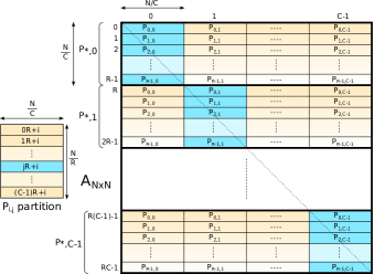
Figure 1: Two-dimensional partitioning of an adjacency matrix $A$ with an $R\times C$ processor grid. The matrix is divided into $C$ consecutive groups of $R\times C$ blocks of edges along the vertical direction. Each block is a $N/(RC)\times N/C$ sub-matrix of $A$. Different groups of blocks are colored with different yellow gradients. For each block, the column of processors owning the corresponding vertices (row indexes) are shown in blue. On the left part, it is shown the sequence of blocks, from top to bottom, assigned to the generic processor $(p_{i},p_{j})$. The colors correspond to the blocks assigned to the processor in each group of blocks.

We implemented a 2D partitioning scheme similar to that described by Yoo et al. in [10], where $RC$ computing nodes are arranged as a logical grid with $R$ rows and $C$ columns and mapped onto the adjacency matrix $A_{N\times N}$, partitioning it into blocks of edges. The processor grid is mapped once horizontally and $C$ times vertically thus dividing the columns in $C$ blocks and the rows in $RC$ blocks, as shown in Figure 1.

Processor $P_{ij}$ handles all the edges in the blocks $(mR+i,\leavevmode\nobreak\ j)$, with $m=0,...,C-1$. Vertices are divided into $RC$ blocks and processor $P_{ij}$ handles the block $jR+i$. Considering the edge lists represented along the columns of the adjacency matrix, this partitioning is such that:

• the edge lists of the vertices handled by each processor are partitioned among the processors in the same grid column;

• for each edge, the processor in charge of the destination vertex is in the same grid row of the edge owner.

Algorithm 1 Parallel BFS with 2D partitioning.

0:  Root vertex $r$.

0:  Processor $P_{ij}$.  

1:  level[:] $\leftarrow-1$

2:  pred[:] $\leftarrow-1$

3:  bmap[:] $\leftarrow 0$

4:  front $\leftarrow\emptyset$

5:  if r belongs to processor $P_{ij}$ then

6:     level[r] $\leftarrow 0$

7:     pred[r] $\leftarrow r$

8:     bmap[r] $\leftarrow 1$

9:     front = $\left\{r\right\}$

10:  end if

11:  lvl $\leftarrow 1$

12:  while true do

13:     front $\leftarrow$ gather front[] from column $j$ //vertical comm

14:     for each u in front do

15:        for each (u,v) in local edge list do

16:           col $\leftarrow$ column of v’s owner

17:           send (u,v) to processor $P_{i,col}$ //horizontal comm

18:        end for

19:     end for

20:     front $\leftarrow\emptyset$

21:     for each received edge (u,v) do

22:        if bmap[v] = 0 then

23:           bmap[v] $\leftarrow 1$

24:           pred[v] $\leftarrow$ u

25:           level[v] $\leftarrow$ lvl

26:           front = front $\cup$ {v}

27:        end if

28:     end for

29:     lvl $\leftarrow$ lvl+1

30:     if front = $\emptyset$ for all processors then

31:        break

32:     end if

33:  end while

With a similar decomposition, each step of the BFS requires two communication phases, called expand and fold. The first one involves the processors in the same grid column whereas the second those in the same grid row. Algorithm 1 shows a pseudo code for a parallel BFS with 2D decomposition. At the beginning of the each step, each processor has its own subset of the frontier set of vertices (initially only the root vertex). The search entails the scanning of the edge lists of all the frontier vertices. Due to property (i) of the 2D decomposition, each processor gathers the frontier sets of vertices from the other processors in the same processor-column (vertical exchange, line 13). The frontier is then expanded by having each column of processors to collectively scan the edge lists of the gathered sets of vertices in search of edges leading to unvisited neighbors. For property (ii), edges found are sent to the processors, in the same grid row, that own the destination vertices (horizontal exchange, lines 14-19). Unvisited destination vertices of the received edges form the frontier of the next BFS step (lines 20-28). The search ends when the frontier of each processor is empty, meaning that the whole connected component containing the root vertex has been visited [12].

The main advantage of the 2D partitioning is a reduction of the number of communications. If $P$ is the number of processors, our first implementation required $O(P)$ data transfers at each step whereas the 2D partitioning only requires $2\times O(\sqrt{P})$ communications.

3 BFS on a multi-GPU system with 2D partitioning

Our work loosely follows the Graph500 [13] benchmark specifications. The benchmark requires to generate in advance a list of edges with an R-MAT generator [14] and to measure the performances over 64 BFS operations started from random vertices. It poses no constraint about the kind of data structures used to represent the graph but it requires the vertices to be represented using at least 48 bits. Since the focus of the present work is the evaluation of the new local part of the search and the 2D partitioning with respect to our original code, we do not strictly adhere to the Graph500 specifications and represent vertices with 32 bits (more than enough to index the highest number of vertices storable in the memory of current GPUs).

3.1 Local graph data structure

Each processor stores its part of the adjacency matrix as a $(N/R)\times(N/C)$ local matrix (Figure 1) where blocks of edges are stored in the same row order as in the global matrix. This allows to map global indexes to local indexes so that global row $v$ is mapped to the same local row for every processor in the same processor-row of the owner of vertex $v$. In a similar way, global column $u$ is mapped to the same local column for every processor in the same processor-column handling the adjacency list of vertex $u$.

Local adjacency matrices are sparse as the global matrix, so they are stored in compressed form. Since they are accessed by reading an entire column for each vertex of the frontier, we used a representation that is efficient for column access, the Compressed Sparse Column (CSC) format. As a consequence, processors may scan adjacency lists by accessing blocks of consecutive memory locations during the frontier expansion (one block for each vertex in the frontier of the same processor-column). Since the non-zeroes entries of an adjacency matrix have all the same value, the CSC is represented with only two arrays: the column offset array col and the row index array row.

Predecessors and BFS levels are stored in arrays of size $N/R$ (number of rows of the local matrix). For the frontier, since it can only contain local vertices, we use an array of size $N/(RC)$ and the information about visited vertices is stored in a bitmap with $\lceil\frac{N/R}{32}\rceil$ 32-bit words.

3.2 Parallel multi-GPU implementation

The code may generate a graph by using the R-MAT generator provided by the reference code available from the Graph500 website. Then the graph is partitioned as described in Section 2.2. The BFS phase is performed entirely by the GPUs with the CPUs acting as network coprocessors to assist in data transfers.

Algorithm 2 shows the code scheme of the BFS phase. Every processor starts with the level, predecessor and bitmap arrays set to default values (lines 1-4). The owner of the root vertex copies its local column index into the frontier array and sets its level, predecessor and visited bit (lines 5-10). All the data structures are indexed by using local indexes. At the beginning of each step of the visit, the expand communication is performed (line 13). Every processor exchanges its frontier with the other processors in the same processor-column and stores the received vertices in the all_front array. Note that in this phase, since processors send subsets of their own vertices, only disjoint sets are exchanged. After the exchange, in the expand_frontier routine, processors in each column collectively scan the whole adjacency lists of the vertices in all_front (line 14). For each vertex, its unvisited neighbors are set as visited and the vertex is set as their predecessor. For neighbors owned locally the level is also set. The routine returns the unvisited neighbors, divided by the processor-column of the owner, inside an array with $C$ blocks, dst_verts.

Algorithm 2 GPU version of Parallel BFS.

0:  Root vertex $r$.

0:  CSC=(row[],col[]).

0:  Processor $P_{ij}$.  

1:  level[:] $\leftarrow-1$

2:  pred[:] $\leftarrow-1$

3:  bmap[:] $\leftarrow 0$

4:  front $\leftarrow[]$

5:  if r belongs to $P_{ij}$ then

6:     level[LOCAL_ROW(r)] $\leftarrow 0$

7:     pred[LOCAL_ROW(r)] $\leftarrow r$

8:     bmap[LOCAL_ROW(r)] $\leftarrow 1$

9:     front[0] $\leftarrow$ LOCAL_COL($r$)

10:  end if

11:  lvl $\leftarrow 1$

12:  while true do

13:     all_front $\leftarrow$ expand_comm(front)

14:     dst_verts $\leftarrow$ expand_frontier(row, col, level, pred, bmap, all_front)

15:     front[:] $\leftarrow$ dst_verts[$j$][:]

16:     dst_verts[$j$] $\leftarrow$ []

17:     int_verts $\leftarrow$ fold_comm(dst_verts)

18:     front $\leftarrow$ front $\oplus$ update_frontier(row, col, level, pred, bmap, int_verts)

19:     if len(front) = $0$ for all processors then

20:        break

21:     end if

22:     lvl $\leftarrow$ lvl$+1$

23:  end while

After the frontier expansion, neighbors local to the processor are moved from the $j$-th block of the dst_verts array into the front array (lines 15-16) and the fold communication phase is performed. Unvisited neighbors just discovered are sent to their owners, located in the same processor-row, and received vertices are returned in the int_verts array (line 17). Finally, the update_frontier routine selects, among the received vertices, those that have not been visited yet and sets their level and bitmap bit (line 18). Returned vertices are then appended to the new frontier and the cycle exit condition is evaluated (line 19). The BFS continues as long as at least one processor has a non-empty frontier at the end of the cycle.

The output is validated by using the same procedure included in our original code.

3.3 Communications

The expand and fold communication phases are implemented with point-to-point MPI primitives and make use of the following scheme:

• start send operations;

• wait for completion of receive operations posted in the previous round;

• post non-blocking receive operations for the next round.

that hides the latency of the receive operations in the BFS round and avoids possible deadlocks due to the lack of receive buffers.

Since the communication involves only local indexes, the expand and fold phases are carried out by exchanging 32-bit words.

3.4 Frontier expansion

After the local frontiers have been gathered, the frontier expansion phase starts. This phase has a workload proportional to the sum of the degrees of the vertices in the current frontier. There are no floating point operations, just few integer arithmetic operations, mainly for array indexing, and it is memory bandwidth bound with an irregular memory access pattern. It is characterized by a high degree of intrinsic parallelism, as each edge originating from the frontier can be processed independently from the others. There could be, however, groups of edges leading to the same vertex. In those cases, only one edge per group should be processed. In our code we use a thread for each edge connected to the frontier and this allows the selection of the single edge to be followed in, at least, two ways: either by taking advantage of benign race conditions or by using synchronization mechanisms such as atomic operations.

In our previous work, we chose to avoid atomic operations because they were quite penalizing with the Nvidia Fermi architecture, available at that time. The current architecture, code-named Kepler, introduced many enhancements including a significant performance improvement of the atomic operations (almost an order of magnitude with respect to Fermi GPUs). As a consequence, we decided to use atomics in the new 2D code. The resulting code is much simpler because there is no longer the need to support the benign race conditions on which the original code relied [8]. Atomics are used to access the bitmap in both the frontier expansion and update phases and to group outgoing vertices based on destination processors.

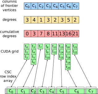
Figure 2: Threads to data mapping assigning one thread per edge. From top to bottom, the first array represents the local column indexes corresponding to frontier vertices. The second contains the local degrees of each vertex, i.e. the number of non-zeroes per column (23 in total), and the third one is the cumulative degree array. The CUDA grid is launched with (at least) 23 threads. By searching the cumulative array for the greatest entry less than its global id, each thread finds its frontier vertex. Finally, threads mapped to the same frontier vertex process its edge list (a CSC column).

At the beginning of the expansion phase, the vertices in the blocks of the all_front array are copied in a contiguous block of device memory and then the corresponding columns of the CSC matrix are processed. We employ a mapping between data and threads similar to the one used in our previous code [8] where a CUDA thread is used for every edge originating from the current frontier. The mapping allows to achieve an optimal load balancing as edge data are evenly distributed among the GPU threads. Given the frontier vertices $u_{0},u_{1},u_{2},...,u_{n-1}$ with degrees $d_{0},d_{1},d_{2},...,d_{n-1}$ and adjacency lists:

$$v^{0}_{0},v^{0}_{1},...,v^{0}_{d_{0}-1}|v^{1}_{0},v^{1}_{1},...,v^{1}_{d_{1}-1}|...|v^{n-1}_{0},v^{n-1}_{1},...,v^{n-1}_{d_{n-1}-1}$$

thread $i$ is mapped onto the $j$-th edge connected to vertex $u_{k}$:

$$i\leavevmode\nobreak\ \leavevmode\nobreak\ \leftrightarrow\leavevmode\nobreak\ \leavevmode\nobreak\ (u_{k},v^{k}_{j})$$

$$k=max\left\{l\leavevmode\nobreak\ \middle|\leavevmode\nobreak\ \sum_{s=0}^{l}d_{s}\leq i,\leavevmode\nobreak\ \forall l<n\right\}\leavevmode\nobreak\ \leavevmode\nobreak\ \leavevmode\nobreak\ \leavevmode\nobreak\ j=i-\sum_{s=0}^{k}d_{s}$$

After vertices in all_front are copied to device memory, we use their degrees to compute a cumulative degree array by means of an exclusive scan operation. The frontier expansion kernel is then launched with $r=\sum_{s=0}^{n-1}d_{s}$ threads. Each thread processes one local edge $(u,v)$ originating from the frontier, i.e. one element of column $u$ of the CSC (see Figure 2). Algorithm 3 shows the pseudo code for the frontier expansion kernel. The source vertex $u$ is found by performing a binary search for the greatest index $k$ such that cumul[k] is less than or equal to the global thread id (line 2) and by accessing the $k$-th location of the frontier array (line 3) [15].

The column offset of vertex $u$ is found in the $u$-th element of the CSC column index array col. The row offset of the destination vertex is computed by subtracting from the thread id the degrees of the vertices preceding $u$ in the frontier array. Finally, the local id $v$ of the destination vertex is found by accessing the CSC row index array at the location corresponding to the sum of both the column and the row offsets (line 4).

The status of the neighbor $v$ is then checked (lines 5-6). If the vertex has already been visited, then the thread returns. Otherwise, it is marked as visited with an atomicOr operation (line 7). That instruction returns the value of the input word before the assignment. By checking the vertex bit in the return value, it is possible to identify the first of different threads handling edges leading to the same vertex (assigned to different columns) that set the visited bit (line 8). Only the first thread proceeds, the others return.

The bitmap is used not only for the vertices owned locally but also for those, belonging to other processors (in the same processor-row), that are reachable from local edges. In other words, the bitmap has an entry for each row of the CSC matrix. This makes possible to send external vertices just once in the fold exchanges because those vertices are sent (and marked in the bitmap) only when they are reached for the first time in the frontier expansion phase.

Algorithm 3 CUDA atomic-based frontier expansion kernel.

0:  frontier[].

0:  current level.

0:  dst_cnt[]=0.

0:  cumulative degree array cumul[].

0:  Processor $P_{ij}$.

0:  CSC=(row[],col[]), bmap[], level[] and pred[].  

1:  gid $\leftarrow$ (blockDim.x*blockIdx.x + threadIdx.x)

2:  k $\leftarrow$ binsearch_maxle(cumul, gid)

3:  u $\leftarrow$ frontier[k]

4:  v $\leftarrow$ row[col[u] + gid - cumul[k]]

5:  m $\leftarrow$ 1 << (v $\bmod$ 32)

6:  if (bmap[v/32] & m) return

7:  q $\leftarrow$ atomicOr(&bmap[v/32], m)

8:  if !(m & q) then

9:     $tgtj\leftarrow$ v/(N/(RC))

10:     off $\leftarrow$ atomicInc(&dst_cnt[$tgtj$])

11:     if ($tgtj$ != $j$) then

12:        dst_verts[$tgtj$][off] $\leftarrow$ v

13:     else

14:        dst_verts[$j$][off] $\leftarrow$ ROW2COL(v)

15:        lvl[v] $\leftarrow$ level

16:     end if

17:     pred[v] $\leftarrow$ u

18:  end if

Each unvisited neighbor is added to the array associated to the processor-column of its owner processor in preparation for the subsequent fold exchange phase (lines 12 and 14). The processor-column is computed based on the local index of the neighbor (line 9) and the counter for such column is atomically incremented to account for multiple threads appending for the same processor (line 10). If the neighbor belongs to the local processor its level is also set (line 15). Finally, regardless of the owner, the neighbor predecessor is set (line 17).

After the kernel has completed, the array containing the discovered vertices (grouped by owner) is copied to host memory in preparation for the fold communication phase.

The bitmap, level and predecessor arrays are never copied back to the host because they are used only by GPU kernels.

3.4.1 Optimizations

In the current CUDA implementation, we introduced an optimization to mitigate the cost of the binary searches performed at the beginning of the frontier expansion kernel. Since threads search for their global index in the cumulative array, non-decreasing indexes are returned to consecutive threads:

$$\verb|binsearch_maxle(cumul, gid)|\leq$$

$$\verb|binsearch_maxle(cumul, gid+1)|$$

Where gid is the global thread identifier that is equal to:

$$\verb|threadIdx.x + blockIdx.x * blockDim.x|$$

That relation makes possible to scan the columns with fewer threads than the number of edges originating from the frontier without increasing the number of binary searches performed per thread. This is done by assigning each thread to a group of consecutive elements in the CSC columns. If not enough elements are available in the column, the group overlaps on the next column. Then, each thread performs a binary search only for its first edge to obtain a base column index. The indexes for subsequent edges $tid+i$ are found by incrementing the base index until $(tid+i)\geq cumul[base+1]$. The overhead introduced by these linear searches is very limited because the majority of edge groups are contained in a single column and so the base column index is never incremented.

Among other optimizations, there is the passage of read-only arrays to kernels with the modifiers const/restrict. In this way the compiler uses the read-only data cache load functions to access them. Moreover, in order to increase instruction-level parallelism, edges assigned to a thread are not processed sequentially, one after the other. Instead, they are processed together in an interleaved way by replacing each kernel instruction with a sequence of independent instructions, one for each edge. In this way, since threads do not stall on independent instructions, each group is executed in a way that hides arithmetic and memory latencies.

Figure 3 reports the total time spent in the frontier expansion kernel to perform single-GPU BFSs with a variable number of edges per thread on an R-MAT graph with scale=$21$ . The maximum performance is obtained by assigning four edges per thread with a performance gain of ${\sim}40\%$ with respect to the case with a thread per neighbor.

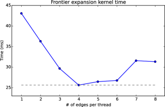
Figure 3: Frontier expansion times measured visiting an R-MAT graph with scale=${21}$ using a single GPU and varying the number of edges per GPU thread.

3.5 Frontier update

In the frontier update phase, local vertices remotely discovered and received during the fold exchange, are processed to find those that are locally unvisited, i.e., whose visited bit is not set.

Since this phase processes the vertices received, instead of their adjacency lists, fewer computational resources are required compared to those necessary in the frontier expansion phase.

As in the expand communication phase, vertices returned by the fold exchange are grouped by sender in different blocks and thus, before starting the processing, they are copied to device memory in contiguous locations.

After the copy, the frontier update kernel is launched with a thread per vertex. Threads are mapped linearly onto the arrays of vertices and each thread is responsible of updating the level and predecessor of its vertex, if unvisited, and to add it to the output array. As in the frontier expansion kernel, we make use of atomic operations in order to synchronize the accesses to the bitmap and the writes to the output buffer. As to the predecessor, since in the fold phase we do not transmit source vertices, the thread, lacking this information, stores the sender processor-column in the predecessor array (the sender saved the predecessor).

After the kernel has completed, the output array is copied to host memory and it is appended to the frontier array.

4 Results

The performances hereafter reported have been obtained on the Piz Daint system belonging to the Centro Svizzero di Calcolo Scientifico (CSCS). Piz Daint is a hybrid Cray XC30 system with 5272 computing nodes interconnected by an Aries network with Dragonfly topology. Each node is powered by both an Intel Xeon E5-2670 CPU and a NVIDIA Tesla K20X GPU and is equipped with 32 GB of DDR3 host memory and 6 GB of GDDR5 device (GPU) memory. The code has been built with the GNU C compiler version 4.8.2, CUDA C compiler version 5.5 and Cray MPICH version 6.2.2. For the GPU implementation of the exclusive scan we used the CUDA Thrust library [16], a well-known, high performance template library implementing a rich collection of data parallel primitives.

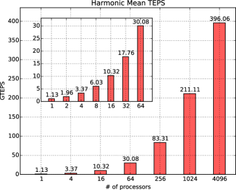
Figure 4: Harmonic mean TEPS measured with a number of GPUs ranging from 1 to 4096 keeping the graph scale per processor fixed.

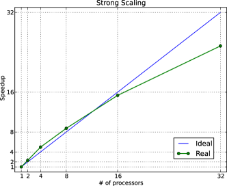
Figure 5: Speedup of the 2D code measured by visiting an R-MAT graph with scale=${25}$.

# of GPUs	grid size	scale	edge factor	# of GPUs	grid size	scale	edge factor
1	$1\times 1$	21		128	$8\times 16$	28
2	$1\times 2$	22		256	$16\times 16$	29
4	$2\times 2$	23		512	$16\times 32$	30
8	$2\times 4$	24	16	1024	$32\times 32$	31	16
16	$4\times 4$	25		2048	$32\times 64$	32
32	$4\times 8$	26		4096	$64\times 64$	33
64	$8\times 8$	27

Table 1: Processor grid and R-MAT graph configurations used for the tests.

The code uses 32-bit data structures to represent the graph because the memory available on a single GPU is not sufficient to hold $2^{32}$ or more edges and it transfers 32-bit words during the communications because the frontier expansion/update and expand/fold communications work exclusively on local vertices. We use 64-bit data only for graph generation/read and partitioning. For the generation of R-MAT graphs we use the make_graph routine found in the reference code for the Graph500 benchmark. The routine returns a directed graph with $2^{scale}$ vertices and ${\sim}edge\_factor\times 2^{scale}$ edges. We turn the graph undirected by adding, for each edge, its opposite. Most of the following results are expressed in Traversed Edges Per Second (TEPS), a performance metric defined by the Graph500 group as the number of input edge tuples within the component traversed by the search, divided by the time required for the BFS to complete, starting right after the graph partitioning. The tests have been performed with both R-MAT generated and real-world graphs. Table 1 reports the processor-grid configurations, scales and edge factors used for R-MAT graphs.

Figure 4 shows the weak scaling plot obtained by using a number of GPUs ranging from 1 to 4096. In order to maintain a fixed problem size per GPU, the graph scale has been increased by 1 for each doubling of the number of processors, starting from scale 21 whereas the edge factor had been set equal to 16 (we set the scale equal to 21 because it is the maximum value that can be used in the 1D implementation, against which we compare many results). For each scale, we report the harmonic mean of the TEPS measured in 64 consecutive BFS operations (a different root vertex is chosen at random for each search). The code scales up to 4096 GPUs where the performances reaches ${\sim}400$ GTEPS on a graph with $2^{33}$ vertices and ${\sim}280$ billions of directed edges. Figure 5 shows the strong scaling plot obtained by visiting a fixed R-MAT graph with scale 25 and edge factor 16 with an increasing number of GPUs. Here we used the maximum scale that fits on a single GPU, to have more work to be done when the number of processes increases. The code scales linearly up to 16 GPUs. With 32 processors, the cost of data transfers becomes comparable to the cost of computations and with more GPUs the advantage becomes marginal and the efficiency drops.

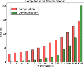
Figure 6: Computation and transfer times (left and right bar, respectively) for BFS operations performed with variable number GPUs on R-MAT graphs.

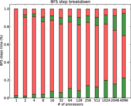
Figure 7: Breakdown plot of the four phases of the BFS (from the bottom to the top of the bars): expand exchange, frontier expansion, fold exchange and frontier update.

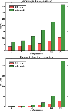
Figure 8: Comparison of computation (upper plot) and communication (lower plot) times between the new code based on 2D decomposition and our original code. Both codes have been run on graphs as specified in the Table 1.

Figure 9: Comparison of the time required by the frontier expansion phase in the new code and the original code. The former is based on atomic operations whereas the latter uses scatter/compact parallel primitives to support benign race conditions.

# of GPUs	Tesla S2050	Tesla K20X
1	0.48	1.13

Table 2: GTEPS obtained by running the 2D code on a Tesla S2050 (Fermi) and on a Tesla K20X (Kepler) using an R-MAT graph with scale $21$ and edge factor $16$.

Data Set Name	Vertices	Edges	Scale	EF	GPUs	GTEPS
com-LiveJournal	3997962	34681189	$\sim 22$	$\sim 9$	2	0.77 (0.43)
soc-LiveJournal1	4847571	68993773	$\sim 22$	$\sim 14$	2	1.25 (0.47)
com-Orkut	3072441	117185083	$\sim 22$	$\sim 38$	4	2.67 (1.43)
com-Friendster	65608366	1806067135	$\sim 25$	$\sim 27$	64	15.68 (5.55)

Table 3: BFS performance of the 2D code with real-world graphs from the Stanford collection. For each graph are reported the number of vertices, of edges, and the (approximate) scale and edge factor (to facilitate the comparison with RMAT graphs). Each traversal has been performed 64 times starting from random vertices, with the specified number of GPUs. Performance reported are the harmonic means of the TEPS measured in the traversals. Within parenthesis are reported the performance figures of the original code.

Figure 6 reports the compute and transfer times of the code. The compute time is the aggregate time required by the frontier expansion and update phases to process the data received in the communication phases. Keeping the problem size per processor fixed, the amount of data received by any process (remote frontiers and discovered vertices) grows with the row and column sizes of the processor grid. For that reason, when the number of processors grows also the amount of data to be exchanged increases, and so it does the execution time. Transfer time includes the time spent in the expand and fold exchanges and in the allreduce operation at the end of the BFS loop. Up to 2048 GPUs, data transfers require less than half of the total BFS time. With 4096 GPUs the communications become dominant and take almost $60\%$ of the total search time. Above 4096 GPUs, we do not expect the code to scale anymore but we did not test it directly.

In Figure 7 it is reported the timing breakdown of the four steps performed in the BFS round: expand exchange, frontier expansion, fold exchange and frontier update. Times are summed across the BFS steps and averaged across 64 operations. By increasing the number of processors, the time required by the frontier expansion phase reduces and, as expected, the weight of the communications increases, becoming dominant with 4096 GPUs. The time required by the frontier update phase is always much smaller than the time spent in the frontier expansion. With any configuration, it accounts for less than $10\%$ of the total time required by the four steps.

In Figure 8 we report the comparison of computation and communication times between our original code and the new one, both run on the Piz Daint cluster. For what concerns the communications (right plot), the advantage of 2D partitioning is apparent with any number of GPUs up to 1024, where 2D transfers are almost eight times faster than those in the original code. For what concerns the computations, with 1024 GPUs the 2D code is ${\sim}3.5$ times faster. This advantage is mainly due to the performance improvement of the atomic operations implemented in the Kepler architecture. Figure 9 shows a comparison of frontier expansion times between our present code using atomics and our original code. Starting from $16$ GPUs, the frontier expansion performed with atomic operations is $2$ times faster than our original approach supporting benign race conditions.

In Table 2, we report the performance of the 2D code obtained on a single GPU with both the Fermi and Kepler architectures. The code runs more than twice as fast on the Kepler GPU.

Finally, Table 3 reports the results obtained traversing real-world graphs obtained from the Stanford Large Network Dataset Collection [17]. Among them we selected undirected graphs with the highest number of edges.

5 Latest Communication optimization

The results presented in Section 4 (Figures 6, 7) show that the communication times steadily grow and eventually exceed the compute time using 4096 nodes. In order to reduce communications cost we reduced the number of vertices exchanged by using a bitmap to keep track of the visited status of both local and non-local vertices. To further reduce the size of the messages we decided to fit to our code an approach proposed in [11, 18] consisting in using bitmaps also for data transfers. The idea is that when the size of vertices lists to be sent exceeds, in bits, the number of indices local to the receiving process, then it is more convenient to send a bitmap with the bits corresponding to the outgoing vertices set. This technique reduces the communication times by limiting the data transmitted to a fixed amount whenever the number of vertices to be transferred would grow over a given threshold. Obviously, that happens in the most expensive steps of the visit. Assuming that the indices to be transferred are 32-bit words and that the size of the subgraph per processor is fixed and equal to $SCALE=21$ we have that the bitmap size is, regardless of the number of processors:

$$size_{b}=\frac{1}{8}\frac{N}{RC}bytes=256kb$$

With respect to the number of vertices, the threshold $T$ over which it is more convenient to use a bitmap is:

$$T=\frac{size_{b}}{4}=65536$$

Whenever a list with more than $T$ vertices needs to be sent, just $256$Kb of data are actually sent, independently of the size of the list (that can grow up to $8$Mb in the example above). This chance applies to both the frontier expansion and fold phases.

In order to maximize the benefits, it is necessary to use the bitmaps only when the number of vertices in the list exceeds the threshold $T$.

We implemented a simple mechanism to dynamically switch between the two representations, using the most convenient alternative for the two transfer procedures at each step of the visit. It is worth noting that with R-MAT graphs the switching point happens during the BFS step, between the expand and the fold phases. This is in accordance to the analysis of the expansion and contraction of the frontier reported by previous studies [3, 4, 19].

For what concerns the packing/unpacking of the vertices lists into/from bitmaps, we used two different approaches. The packing has been implemented into specialized versions of the frontier expansion and update kernels that directly produce bitmaps instead of lists. For the unpacking, we developed specific warp-centric kernels based on the Kepler’s shuffle instructions. The overhead introduced by these kernels is negligible with respect to the frontier expansion/update kernels and largely compensated by the dramatic reduction of the data-exchange times that it makes possible.

The impact of this optimization on the overall performance is remarkable and leads to a net 2x speed-up in the number of TEPS as shown in Figure 10. Figure 11 reports the aggregated computation and communication times of the code using the bitmaps. The drop of communication times from ${\sim}200$ms to ${\sim}40$ms with 4096 GPUs is an indication that the code may scale even on larger GPU clusters.

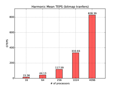
Figure 10: Harmonic mean TEPS measured with a number of GPUs ranging from 1 to 4096 keeping the graph scale per processor fixed and taking advantage of the bitmap optimization.

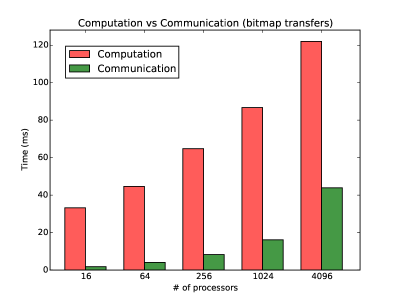
Figure 11: Computation and transfer times (left and right bar, respectively) for BFS operations performed with variable number GPUs on R-MAT graphs taking advantage of the bitmap optimization.

6 Related works

In recent years high performance implementations of graph algorithms have attracted much attention. Several works tackled the issues related to both shared memory and distributed memory systems.

On the single GPU different solutions have been proposed to address workload imbalance among threads. The naive assignment, in which each thread is assigned to one element of the BFS queue, may determine a dramatic unbalance and poor performances [8]. It is also possible to assign one thread to each vertex of the graph but, as showed by Harish et al. [20], the overhead of having a large number of unutilized threads results in poor performances. To solve this problem, Hong et al. [2, 21] proposed a warp centric programming model. In their implementation each warp is responsible of a subset of the vertices in the BFS queue. Another solution has been proposed in the work of Merrill et al. [3]. They assigned a chunk of data to a CTA (a CUDA block). The CTA works in parallel to inspect the vertices in its chunk.

We devised an original data mapping described in [8]. Then, to reduce the work, we used an integer map to keep track of visited vertices. Agarwal et al. [1], first introduced this optimization using a bitmap that has been used in almost all subsequent works.

On distributed memory systems many recent works rely on a linear algebra based representation of graph algorithms [5, 22, 18, 23].

Ueno et al. [22] presented a hybrid CPU-GPU implementation of the Graph500 benchmark, using the 2D partitioning proposed in [10]. Their implementation uses the technique introduced by Merrill et al. [3] to create the edge frontier and resort to a novel compression technique to shrink the size of messages. They also implemented a sophisticated method to overlap communication and computation in order to reduce the working memory size of the GPUs.

A completely different algorithm that uses a direction-optimizing approach has been proposed by Beamer et. al [4] and extended in [23] for a cluster of CPUs. The direction-optimizing method switches between the top-down and the bottom-up traversal. The bottom-up search dramatically reduces the number of traversed edges during the most expensive computational levels of the BFS by searching the parent in the frontier starting from the sub-set of unvisited vertices. The parent search implies a serialization in order to minimize the required work. However, on shared memory systems (including single GPUs [24, 19]) the BFS performance increases significantly.

A recent work [7] demonstrates the chance of having an effective implementation of a distributed direction-optimizing approach on the BlueGene/P by using a 1D partitioning. That partitioning simplifies the parallelization of the bottom-up algorithm but it may require a significant increase in the number of communications. Their results show that the combination of the underlaying architecture and the SPI interface is well suited to the purpose. The authors report that replacing the SPI with MPI incurs a loss of performance by a factor of nearly 5 although the MPI-based implementation cannot be considered optimal. This suggests that the scalability of a distributed implementation may be worse on different network architectures.

The work presented in [25] achieves an outstanding speed-up for the implementation of a direction-optimizing BFS on a single GPU, nearly six times faster than more recent implementations [19, 24]. However, it also shows a very poor scalability on a multi-GPUs system.

It should be also taken into account that the bottom-up approach may not be a viable option if an actual traversal of all the edges in a connected component is required.

Satish et al. [11] implemented a distributed BFS with 1D partitioning that shows remarkable scaling properties up to 1024 nodes. They devised a technique to delay the exchange of predecessors. We implemented the same technique independently, as reported in [9], and use it in the present work.

Compared with state-of-the-art implementations on distributed architectures, our implementation on 4096 GPUs is 2.6 times faster than the distributed GPU implementation in [22] that uses 4096 GPUs and 1366 CPUs, 3.4 times faster than the distributed bottom-up in [23] that uses up to 115000 cores and 3.3 times faster than the 2D implementation in [18] that uses 4096 BlueGene/Q nodes. To the best of our knowledge, the work in [7] achieves the best performance.

7 Conclusions

We presented the performance results of our new parallel code for distributed BFS operations on large graphs. The code employs a 2D partitioning of the adjacency matrix for efficient communications and uses CUDA to accelerate local computations. The computational core is based on our previous work on GPU graph processing and is characterized by optimal load balancing among GPU threads, taking advantage of the efficient atomic operations of the Kepler architecture.

We further enhanced the code by using a bitmap to reduce the data exchanged among processors during the most expensive BFS steps. This optimization, improved the performances up to a factor 2 with 4096 GPUs.

The result is a code that shows good scalability up to $4096$ Nvidia K20X GPUs, visiting $830$ billion edges per second of an R-MAT graph with $2^{33}$ vertices and ${\sim}280$ billions of directed edges. We compared the performances of the new code with those of the original one, which relied on a combination of parallel primitives in place of atomic operations, on the same cluster of GPUs. The 2D code is up to eight times faster on R-MAT graphs of the same size.

References

- [1] V. Agarwal, F. Petrini, D. Pasetto, and D.A. Bader. Scalable graph exploration on multicore processors. In High Performance Computing, Networking, Storage and Analysis (SC), 2010 International Conference for, pages 1 –11, nov. 2010.
- [2] T. Oguntebi S. Hong, S. K. Kim and Kunle Olukotun. Accelerating cuda graph algorithms at maximum warp. In Proceedings of the 16th ACM symposium on Principles and practice of parallel programming, 2011.
- [3] Duane Merrill, Michael Garland, and Andrew Grimshaw. Scalable gpu graph traversal. In Proceedings of the 17th ACM SIGPLAN Symposium on Principles and Practice of Parallel Programming, PPoPP ’12, pages 117–128, New York, NY, USA, 2012. ACM.
- [4] Scott Beamer, Krste Asanović, and David Patterson. Direction-optimizing breadth-first search. In Proceedings of the International Conference on High Performance Computing, Networking, Storage and Analysis, SC ’12, pages 12:1–12:10, Los Alamitos, CA, USA, 2012. IEEE Computer Society Press.
- [5] Aydin Buluc and Kamesh Madduri. Parallel breadth-first search on distributed memory systems. SC ’11 Proceedings of 2011 International Conference for High Performance Computing, Networking, Storage and Analysis, 2011.
- [6] Koji Ueno and Toyotaro Suzumura. Highly scalable graph search for the graph500 benchmark. In Proceedings of the 21st international symposium on High-Performance Parallel and Distributed Computing, HPDC ’12, pages 149–160, New York, NY, USA, 2012. ACM.
- [7] Fabio Checconi and Fabrizio Petrini. Traversing trillions of edges in real time: Graph exploration on large-scale parallel machines. In Proceedings of the 2014 IEEE 28th International Parallel and Distributed Processing Symposium, IPDPS ’14, pages 425–434, Washington, DC, USA, 2014. IEEE Computer Society.
- [8] Massimo Bernaschi and Enrico Mastrostefano. Efficient breadth first search on multi-gpu systems. Journal of Parallel and Distributed Computing, 73:1292 – 1305, 2013.
- [9] Massimo Bernaschi, Giancarlo Carbone, Enrico Mastrostefano, and Flavio Vella. Solutions to the st-connectivity problem using a gpu-based distributed BFS. Journal of Parallel and Distributed Computing, in press, 2014.
- [10] Andy Yoo, Edmond Chow, Keith Henderson, William McLendon, Bruce Hendrickson, and Umit Catalyurek. A scalable distributed parallel breadth-first search algorithm on bluegene/l. In Supercomputing, 2005. Proceedings of the ACM/IEEE SC 2005 Conference, pages 25–25. IEEE, 2005.
- [11] Nadathur Satish, Changkyu Kim, Jatin Chhugani, and Pradeep Dubey. Large-scale energy-efficient graph traversal: A path to efficient data-intensive supercomputing. In Proceedings of the International Conference on High Performance Computing, Networking, Storage and Analysis, SC ’12, pages 14:1–14:11, Los Alamitos, CA, USA, 2012. IEEE Computer Society Press.
- [12] In order to reduce the amount of exchanged data, in the fold phase we send only destination vertices, instead of edges. moreover, to avoid sending more than once the same vertex to its owner, we use a bitmap to keep track of local vertices that have been visited.
- [13] Graph 500 benchmark (www.graph500.org).
- [14] Deepayan Chakrabarti, Yiping Zhan, and Christos Faloutsos. R-mat: A recursive model for graph mining. Computer Science Department. Paper 541. (http://repository.cmu.edu/compsci/541), 2004.
- [15] Since consecutive threads search for consecutive values, sequences of threads mapped onto the same adjacency lists access the same memory locations during the binary search. different sequences share an initial part of the search path whose length depends on their relative distance. as a consequence, the memory access pattern is quite efficient since threads in each sequence perform broadcast memory accesses that are served with single memory transactions, one for each search jump.
- [16] Jared Hoberock and Nathan Bell. Thrust cuda library (http://thrust.github.com/).
- [17] Jure Leskovec. Stanford large network dataset collection (http://snap.stanford.edu/data/index.html).
- [18] Fabio Checconi, Fabrizio Petrini, Jeremiah Willcock, Andrew Lumsdaine, Anamitra Roy Choudhury, and Yogish Sabharwal. Breaking the speed and scalability barriers for graph exploration on distributed-memory machines. In High Performance Computing, Networking, Storage and Analysis (SC), 2012 International Conference for, pages 1–12. IEEE, 2012.
- [19] Yang You, David Bader, and Maryam Mehri Dehnavi. Designing a heuristic cross-architecture combination for breadth-first search. In Parallel Processing (ICPP), 2014 43rd International Conference on, pages 70–79, Sept 2014.
- [20] Pawan Harish and P.J. Narayanan. Accelerating large graph algorithms on the gpu using cuda. In Srinivas Aluru, Manish Parashar, Ramamurthy Badrinath, and ViktorK. Prasanna, editors, High Performance Computing – HiPC 2007, volume 4873 of Lecture Notes in Computer Science, pages 197–208. Springer Berlin Heidelberg, 2007.
- [21] Sungpack Hong, T. Oguntebi, and K. Olukotun. Efficient parallel graph exploration on multi-core cpu and gpu. In Parallel Architectures and Compilation Techniques (PACT), 2011 International Conference on, pages 78 –88, oct. 2011.
- [22] Koji Ueno and Toyotaro Suzumura. Parallel distributed breadth first search on gpu. In HiPC 2013 (IEEE International Conference on High Performance Computing) 2013/12, page To appear, 2013.
- [23] Scott Beamer, Aydın Buluc~̧, Krste Asanović, and David A. Patterson. Distributed memory breadth-first search revisited: Enabling bottom-up search. Technical Report UCB/EECS-2013-2, EECS Department, University of California, Berkeley, Jan 2013.
- [24] Dan Zou, Yong Dou, Qiang Wang, Jinbo Xu, and Baofeng Li. Direction-optimizing breadth-first search on cpu-gpu heterogeneous platforms. In High Performance Computing and Communications 2013 IEEE International Conference on Embedded and Ubiquitous Computing (HPCC EUC), 2013 IEEE 10th International Conference on, pages 1064–1069, Nov 2013.
- [25] Takaaki Hiragushi and Daisuke Takahashi. Efficient hybrid breadth-first search on gpus. In Algorithms and Architectures for Parallel Processing, volume 8286 of Lecture Notes in Computer Science, pages 40–50. Springer International Publishing, 2013.