Robust manipulation of superconducting qubits in the presence of fluctuations

Abstract

Superconducting quantum systems are promising candidates for quantum information processing due to their scalability and design flexibility. However, the existence of defects, fluctuations, and inaccuracies is unavoidable for practical superconducting quantum circuits. In this paper, a sampling-based learning control (SLC) method is used to guide the design of control fields for manipulating superconducting quantum systems. Numerical results for one-qubit systems and coupled two-qubit systems show that the “smart” fields learned using the SLC method can achieve robust manipulation of superconducting qubits, even in the presence of large fluctuations and inaccuracies.

Superconducting quantum circuits based on Josephson junctions are macroscopic circuits, but they can behave quantum mechanically, like artificial atoms, allowing the observation of quantum entanglement and quantum coherence on a macroscopic scale You-and-Nori-2005 ; Wendin-and-Shumeiko-2006 ; Schoelkopf-and-Girvin-2008 ; Clarke-and-Wilhelm-2008 ; You-and-Nori-2011 ; Xiang-et-al-2013 ; Georgescu-et-al-2014 . These artificial atoms can be used to test the laws of quantum mechanics on macroscopic systems and also offer a promising way to implement quantum information technology. Superconducting qubits have been widely investigated theoretically and implemented experimentally in the last fifteen years due to their advantages, such as scalability, design flexibility and tunability, for solid-state quantum computation and quantum simulations You-and-Nori-2005 ; Wendin-and-Shumeiko-2006 ; Schoelkopf-and-Girvin-2008 ; Clarke-and-Wilhelm-2008 ; You-and-Nori-2011 ; Xiang-et-al-2013 ; Georgescu-et-al-2014 ; Pashkin-et-al-2003 ; Steffen-et-al-2010 ; Chiorescu-et-al-2004 ; Wallraff-et-al-2004 ; Wilson-et-al-2007 ; Liu-et-al-2005 ; Valenzuela-et-al-2006 ; Sillanp -et-al-2007 ; Wei-et-al-2008 ; Steffen-et-al-2006 ; Hofheinz-et-al-2009 .

In practical applications, the existence of noise (including extrinsic and intrinsic), inaccuracies (e.g., inaccurate operation in the coupling between qubits) and fluctuations (e.g., fluctuations in magnetic fields and electric fields) in superconducting quantum circuits is unavoidable McDermott-2009 ; Valente-et-al-2010PRB ; Siddiqi-et-al-2012Nature ; Siddiqi-et-al-2012APL ; Siddiqi-et-al-2012PRL ; Khani-et-al-2012PRA ; Paladino-et-al-2014RMP . For simplicity, in this paper we use fluctuations to represent noise, inaccuracies, and fluctuations. These fluctuations degrade the performance of robustness and reliability in superconducting quantum circuits. Hence, it is highly desirable, for the development of practical quantum technology, to design control fields that are robust against fluctuations Pravia-et-al-2003 ; Falci-et-al-2005 ; Montangero-et-al-2007 ; Zhang-et-al-2009 ; Zhang-et-al-2012 ; Wu-et-al-2013 ; Kosut-et-al-2013 .

Robustness has been recognized as one of the key properties for a reliable quantum information processor. Several methods have been developed for enhancing the robustness of quantum systems James-et-al-2007 ; Dong-and-Petersen-2009NJP . One important paradigm is feedback control, where the signal obtained from the system is fed back to adjust input control fields aiming at achieving improved robustness as well as other measures of system performance (e.g., stability) Wiseman-and-Milburn-2009 . A typical example of the feedback paradigm is quantum error correction, where possible errors are corrected based on detection outcomes Gaitan-2008 . Usually, feedback control is difficult to implement in practical quantum systems due to the fast time scale of quantum systems and measurement backaction in the quantum domain. A more feasible paradigm is open-loop control for improving robustness of quantum systems where no feedback signal is required. Dynamical decoupling Viola-et-al-1999 ; Khodjasteh-et-al-2010 and optimal control methods Kosut-et-al-2013 ; Rabitz-et-al-2004 ; Wilhelm-et-al-2007 ; Ginossar-et-al-2010 ; Wilhelm-et-al-2011 ; Wilhelm-et-al-2014 can be used to design robust control fields for manipulating quantum states or quantum gates. In this paper, we develop a “smart” open-loop control method (i.e., sampling-based learning control) to guide the design of robust control fields for superconducting quantum systems. The sampling-based learning control (SLC) method includes two steps of “training” and “testing” Chen-et-al-2013arXiv . In the training step, we obtain some artificial samples by sampling the fluctuation parameters and construct an augmented system using these samples. Then we employ a gradient-flow-based learning algorithm to learn optimal fields for the augmented system. The robustness of the control fields is tested and evaluated using additional samples generated by sampling fluctuation parameters in the testing step. Here we apply the SLC method to several examples of superconducting qubits, including single-charge qubits, two coupled charge qubits and two coupled phase qubits with fluctuations. Our results show that the SLC method can efficiently learn “smart” fields that are insensitive to even 40%$\sim$50% fluctuations. The superconducting quantum circuits with the “smart” fields can run more reliably.

Results

Single charge qubits with fluctuations. In superconducting quantum circuits, the Josephson coupling energy $E_{J}$ and the charging energy $E_{C}$ are two significant quantities. Their ratio determines whether the phase or the charge dominates the behaviour of the qubit, which can form flux qubits or charge qubits You-and-Nori-2005 . The simplest charge qubit is based on a small superconducting island (called a Cooper-pair box) coupled to the outside world through a weak Josephson junction and driven by a voltage source through a gate capacitance within the charge regime (i.e., $E_{C}\gg E_{J}$) You-and-Nori-2005 . The Hamiltonian of the Cooper-pair box can be described as You-and-Nori-2005

$$H=E_{C}(n-n_{g})^{2}-E_{J}\cos\phi$$ (1)

where the phase drop $\phi$ across the Josephson junction is conjugate to the number $n$ of extra Cooper pairs in the box, $n_{g}=C_{g}V_{g}/2e$ is controlled by the gate voltage $V_{g}$ ($C_{g}$ is the gate capacitance and $2e$ is the charge of each Cooper pair). In most experiments, the Josephson junction in the charge qubit is replaced by a dc superconducting quantum interference device (SQUID) to make it easier to control the qubit. In a voltage range near a degeneracy point, the system can be approximated as a qubit with the following Hamiltonian

$$H=f(V_{g})\sigma_{z}-g(\Phi)\sigma_{x}$$ (2)

where $f(V_{g})$ is related to the charging energy $E_{C}$ and this term can be adjusted through external parameters, such as the voltage $V_{g}$, and $g(\Phi)$ corresponds to a controllable term including different control parameters, such as the flux $\Phi$ in the SQUID.

For superconducting qubits in laboratories, the existence of fluctuations is unavoidable (e.g., fluctuations in the Josephson coupling energy and the charging energy, or inaccuracies in the magnetic flux). We assume that possible fluctuations exist in both $f(V_{g})$ and $g(\Phi)$. Suppose that the factors $f(V_{g})$ and $g(\Phi)$ can be controlled by adjusting external parameters. Since $E_{J}$ could be around ten GHz and $E_{C}$ could be around one hundred GHz (e.g., the experiment in Pashkin-et-al-2003 used $E_{J1}=13.4\ \text{GHz}$, $E_{J2}=9.1\ \text{GHz}$, $E_{C1}=117\ \text{GHz}$ and $E_{C2}=152\ \text{GHz}$), we assume $f(V_{g})/\hbar\in[0,40]\ \text{GHz}$ and $g(\Phi)/\hbar\in[0,9.1]\ \text{GHz}$. We could have used 10, instead of 9.1, but we chose 9.1 simply because it was the number used in one experiment. The practical control terms are $\bar{f}(V_{g})=\theta^{z}f(V_{g})$ and $\bar{g}(\Phi)=\theta^{x}g(\Phi)$ (where the fluctuation parameters $\theta^{z}\in[1-\Theta^{z},1+\Theta^{z}]$ and $\theta^{x}\in[1-\Theta^{x},1+\Theta^{x}]$) due to possible multiplicative fluctuations. Here the bounds of fluctuations $\Theta^{z}$ and $\Theta^{x}$ characterize the maximum ranges of fluctuations in $\theta^{z}$ and $\theta^{x}$, respectively. The fluctuations can originate from the fluctuations in the magnetic flux $\Phi$, the voltage $V_{g}$, the Josephson coupling energy $E_{J}$ and the charging energy $E_{C}$.

As an example, we assume that the initial state is $|\psi_{0}\rangle=|g\rangle$, and the target state is either $|\psi_{\text{target}}\rangle=|e\rangle$ or $|\psi_{\text{target}}\rangle=\frac{1}{\sqrt{2}}(|g\rangle+|e\rangle)$. Let the operation time be $T=1\ \text{ns}$. Now we employ the sampling-based learning control method (see the methods Section) to learn an optimal control field for manipulating the charge qubit system from the initial state to a target state. The time interval $t\in[0,1]\ \text{ns}$ is equally divided into $100$ smaller time intervals. Without loss of generality, we assume $\theta^{x}$ and $\theta^{z}$ to have uniform distributions and have the same bound of fluctuations (i.e., $\Theta^{x}=\Theta^{z}$). An augmented system is constructed by selecting $N_{x}=5$ values for $\theta^{x}$ and $N_{z}=5$ values for $\theta^{z}$. The initial control fields are $f(V_{g})/\hbar=\sin t+\cos t+20$ GHz and $g(\Phi)/\hbar=\sin t+\cos t+5$ GHz. The learning algorithm runs for about $7000$ iterations for $|\psi_{\text{target}}\rangle=|e\rangle$ ($4000$ iterations for $|\psi_{\text{target}}\rangle=\frac{1}{\sqrt{2}}(|g\rangle+|e\rangle)$) before it converges to optimal control fields. After the optimal control fields are learned for the augmented system, they are applied to 5000 samples generated by stochastically selecting the values of the fluctuation parameters for evaluating the performance. The fidelity between the final state $|\psi(T)\rangle$ and the target state $|\psi_{\text{target}}\rangle$ is defined as $F(|\psi(T)\rangle,|\psi_{\text{target}}\rangle)=|\langle\psi(T)|\psi_{\text{target}}\rangle|$ Nielsen-and-Chuang-2000 . The relationship between the average fidelity and the bounds of the fluctuations is shown in Fig. 1. Although the performance decreases when increasing the bounds on the fluctuations, the “smart” fields can still drive the system from the initial state $|\psi_{0}\rangle=|g\rangle$ to a given target state with high fidelity (the average fidelity is $\bar{F}=0.9909$ for $|\psi_{\text{target}}\rangle=|e\rangle$, and $\bar{F}=0.9952$ for $|\psi_{\text{target}}\rangle=\frac{1}{\sqrt{2}}(|g\rangle+|e\rangle)$) even though the bound on the fluctuations is $25\%$ (i.e., $50\%$ fluctuations relative to the nominal value).

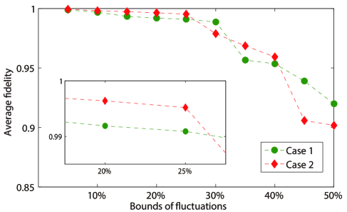
Figure 1: Average fidelity versus the bounds of fluctuations $\Theta^{z}$ and $\Theta^{x}$ for charge qubits. The fluctuation parameters $\theta^{z}$ and $\theta^{x}$ have uniform distributions in $[1-\Theta,1+\Theta]$ (i.e., we assume $\Theta^{z}=\Theta^{x}=\Theta$). Here we consider $|\psi_{0}\rangle=|g\rangle$, and $|\psi_{\text{target}}\rangle=|e\rangle$ (Case 1) or $|\psi_{\text{target}}\rangle=\frac{1}{\sqrt{2}}(|g\rangle+|e\rangle)$ (Case 2). Every average fidelity is calculated using 5000 tested samples.

We also test the relationship between the number of values $N_{f}$ for $\theta^{x}$ and $\theta^{z}$ ($N_{x}=N_{z}=N_{f}$) and the average fidelity for bounds on the fluctuations $\Theta^{z}=\Theta^{x}=15\%$. The performance is shown in Fig. 2. It is clear that the performance is excellent for $N_{f}=5$ or $7$. Although it is possible to improve the performance through using more samples, too many samples will cost more computation resources and spend too much time for learning a set of optimal fields. For example, the laptop Thinkpad T440p, with a CPU of 2.5 GHz, needs about 13 minutes to find the optimal fields for $N_{f}=5$; while this laptop requires about 42 minutes for $N_{f}=11$. When increasing the number of fluctuation parameters, the time consuming quickly increases with the increasing of $N_{f}$. Hence, we choose $N_{f}=5$ for each fluctuation parameter in all of the following numerical results.

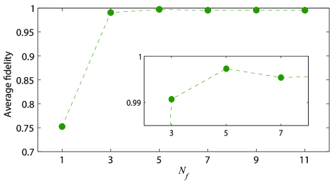
Figure 2: Average fidelity versus the number $N_{f}$ of values for $\theta^{x}$ and $\theta^{z}$ ($N_{f}=N_{x}=N_{z}$). Here, $\Theta^{z}=\Theta^{x}=15\%$ (i.e., 30% fluctuations), $|\psi_{0}\rangle=|g\rangle$ and $|\psi_{\text{target}}\rangle=\frac{1}{\sqrt{2}}(|g\rangle+|e\rangle)$. Every average fidelity is calculated using 5000 samples.

Two coupled qubits with fluctuations.

We first consider the coupled qubit circuit in You-et-al-2003 where a symmetric dc SQUID with two sufficiently large junctions is used to couple two charge qubits (see Fig. 3). Each qubit is realized by a Cooper-pair box with Josephson coupling energy $E_{Jj}$ and capacitance $C_{Jj}$ (j=1, 2). Each Cooper-pair box is biased by an applied voltage $V_{j}$ through the gate capacitance $C_{j}$ ($j=1,2$). We apply a flux $\Phi_{s}$ inside the large-junction dc SQUID loop with two junctions of large $E_{J0}$. The Hamiltonian of the coupled charge qubits can be described as

$$H=f(V_{1})\sigma^{(1)}_{z}+f(V_{2})\sigma^{(2)}_{z}-g(\Phi_{1})\sigma^{(1)}_{x}-g(\Phi_{2})\sigma^{(2)}_{x}-\chi(t)\sigma^{(1)}_{x}\sigma^{(2)}_{x}.$$ (3)

Due to possible fluctuations, we assume that the Hamiltonian for practical systems is

$$H=\theta_{1}f(V_{1})\sigma^{(1)}_{z}+\theta_{2}f(V_{2})\sigma^{(2)}_{z}-\theta_{3}g(\Phi_{1})\sigma^{(1)}_{x}-\theta_{4}g(\Phi_{2})\sigma^{(2)}_{x}-\theta_{5}\chi(t)\sigma^{(1)}_{x}\sigma^{(2)}_{x}$$ (4)

where the fluctuation parameters $\theta_{j}\in[1-\Theta_{j},1+\Theta_{j}]$ ($j=1,2,3,4,5$).

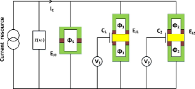
Figure 3: A coupled-qubit circuit with a biased-current source of impedance $Z(\omega)$ You-et-al-2003 . Two charge qubits are coupled by the dc SQUID with two junctions with large $E_{J0}$.

We let $g(\Phi_{1})/\hbar=g(\Phi_{2})/\hbar=9.1\ \text{GHz}$, the control terms $f(V_{1})/\hbar\in[0,40]\ \text{GHz}$, $f(V_{2})/\hbar\in[0,40]\ \text{GHz}$, $|\chi(t)/\hbar|\leq 0.5\ \text{GHz}$ and $\theta_{5}(t)\equiv 1$. The operation time $T=2\ \text{ns}$. We assume that the fluctuation parameters $\theta_{j}$ ($j=1,2,3,4$) may be time varying. Hence, $\theta_{3}$ and $\theta_{4}$ may correspond to time-varying additive fluctuations. The fluctuations in $\theta_{1}$ and $\theta_{2}$ may originate from the time-varying errors in the driving fields. As an illustrative example, we let $\theta_{j}=1-\vartheta_{j}\cos t$, where each $\vartheta_{j}$ has a uniform distribution in the interval $[1-\Theta_{j},1+\Theta_{j}]$. For simplification, we assume $\theta_{1}=\theta_{2}$, $\theta_{3}=\theta_{4}$ and $\Theta_{1}=\Theta_{2}=\Theta_{3}=\Theta_{4}=\Theta$. We now consider a controlled-phase-shift gate operation on an initial state $|\psi_{0}\rangle=\alpha_{1}|g,g\rangle+\alpha_{2}|g,e\rangle+\alpha_{3}|e,g\rangle+\alpha_{4}|e,e\rangle$; i.e., the target state is $|\psi_{\text{target}}\rangle=\alpha_{1}|g,g\rangle+\alpha_{2}|g,e\rangle+\alpha_{3}|e,g\rangle-\alpha_{4}|e,e\rangle$. In particular, we let $\alpha_{1}=0.7$, $\alpha_{2}=0.1$, $\alpha_{3}=0.7i$ and $\alpha_{4}=0.1i$. The time interval $t\in[0,2]\ \text{ns}$ is equally divided into $200$ smaller time intervals. The control fields are initialized as: $f(V_{1})/\hbar=f(V_{2})/\hbar=\sin t+\cos t+5$ GHz, $\chi(t)/\hbar=0.25\sin t$ GHz. The learning algorithm runs for about $5000$ iterations before the optimal control fields are found. Then the learned fields are applied to 5000 samples that are generated by selecting the values of the fluctuation parameters according to a uniform distribution. The performance is shown in Fig. 4. Although the performance decreases when increasing the bounds on the fluctuations, the “smart” fields can still drive the system from the initial state $|\psi_{0}\rangle=0.7|g,g\rangle+0.1|g,e\rangle+0.7i|e,g\rangle+0.1i|e,e\rangle$ to the target state $|\psi_{\text{target}}\rangle=0.7|g,g\rangle+0.1|g,e\rangle+0.7i|e,g\rangle-0.1i|e,e\rangle$ with high fidelity (average fidelity 0.9941) even with $40\%$ fluctuations.

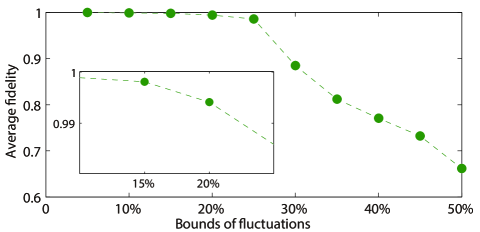
Figure 4: Average fidelity versus the bound on the fluctuations $\Theta$ for two coupled charge qubits with a biased-current source. The fluctuation parameters $\theta_{j}=1-\vartheta_{j}\cos t$ ($j=1,2,3,4$), where each $\vartheta_{j}$ has a uniform distribution in $[1-\Theta,1+\Theta]$. Here we assume $\theta_{1}=\theta_{2}$ and $\theta_{3}=\theta_{4}$. The initial state $|\psi_{0}\rangle=0.7|g,g\rangle+0.1|g,e\rangle+0.7i|e,g\rangle+0.1i|e,e\rangle$ and the target state $|\psi_{\text{target}}\rangle=0.7|g,g\rangle+0.1|g,e\rangle+0.7i|e,g\rangle-0.1i|e,e\rangle$. Each average fidelity is calculated using 5000 samples.

In the two numerical examples of single-charge qubits and two coupled charge qubits, we use some ideal parameter values to show the effectiveness and excellent performance of the proposed method. It is straightforward to extend our method to other systems. Indeed, our proposed method is very flexible in the selection of the operation time $T$ and the target state, and is also robust against fluctuations with different distributions. Here, we consider another example based on the two coupled phase qubits in Ref. Martinis-et-al-2011PRL . Each phase qubit is a nonlinear resonator built from an Al/AlO_x/Al Josephson junction, and two qubits are coupled via a modular four-terminal device (for detail, see Fig. 1 in Martinis-et-al-2011PRL ). This four-terminal device is constructed using two nontunable inductors, a fixed mutual inductance and a tunable inductance. The equivalent Hamiltonian can be described as

$$H=\frac{\hbar\omega_{1}(t)}{2}\sigma^{(1)}_{z}+\frac{\hbar\omega_{2}(t)}{2}\sigma^{(2)}_{z}+\frac{\hbar\omega_{3}(t)}{2}\sigma^{(1)}_{x}+\frac{\hbar\omega_{4}(t)}{2}\sigma^{(2)}_{x}+\frac{\hbar\Omega_{c}(t)}{2}(\sigma^{(1)}_{x}\sigma^{(2)}_{x}+\frac{1}{6\sqrt{N_{1}N_{2}}}\sigma^{(1)}_{z}\sigma^{(2)}_{z})$$ (5)

where $N_{1}$ and $N_{2}$ are the number of levels in the potentials of qubits 1 and 2. The typical values for $N_{1}$ and $N_{2}$ are $N_{1}=N_{2}=5$. Due to possible fluctuations, we assume that the practical Hamiltonian has the following form

$$H=\frac{\hbar\theta_{1}\omega_{1}(t)}{2}\sigma^{(1)}_{z}+\frac{\hbar\theta_{2}\omega_{2}(t)}{2}\sigma^{(2)}_{z}+\frac{\hbar\omega_{3}}{2}\sigma^{(1)}_{x}+\frac{\hbar\omega_{4}}{2}\sigma^{(2)}_{x}+\frac{\hbar\theta_{3}\Omega_{c}(t)}{2}(\sigma^{(1)}_{x}\sigma^{(2)}_{x}+\frac{1}{30}\sigma^{(1)}_{z}\sigma^{(2)}_{z})$$ (6)

with $\theta_{j}\in[1-\Theta,1+\Theta]$ ($j=1,2,3$).

We assume that the frequencies $\omega_{1}(t),\omega_{2}(t)\in[0,5]\ \text{GHz}$ can be adjusted by changing the bias currents of two phase qubits, and $\Omega_{c}(t)\in[-100,100]\ \text{MHz}$ can be adjusted by changing the bias current in the coupler. Let $\omega_{3}=\omega_{4}=2\ \text{GHz}$, the operation time $T=50\ \text{ns}$, and each fluctuation parameter $\theta_{j}$ $(j=1,2,3)$ in (6) has a truncated Gaussian distribution in $[1-\Theta,1+\Theta]$. Assume that the probability density function of the truncated Gaussian distribution is $p(x,\mu,\sigma,l,r)=\phi(\frac{x-\mu}{\sigma})\{\sigma[\Phi(\frac{r-\mu}{\sigma})-\Phi(\frac{l-\mu}{\sigma})]\}^{-1}$, where $\mu=0$, $\sigma=\Theta/3$, $l=-\Theta$, $r=\Theta$, $\phi(x)={(2\pi)}^{-1/2}\text{exp}(-\frac{1}{2}x^{2})$ is the probability density function of the standard normal distribution, and $\Phi(x)$ is its cumulative distribution function.

We now consider a CNOT operation. In particular, we let the initial state be $|\psi_{0}\rangle=\frac{1}{\sqrt{2}}(|g,g\rangle+|e,g\rangle)$ and the target state be a maximum entangled state $|\psi_{\text{target}}\rangle=\frac{1}{\sqrt{2}}(|g,g\rangle+|e,e\rangle)$. In the training step, the fluctuations are uniformly sampled. However, in the testing step the samples are selected by sampling the fluctuation parameters with a truncated Gaussian distribution. For simplicity, we let $\theta_{1}=\theta_{2}$. The initial vaules are $\omega_{1}=\omega_{2}=\sin t+\cos t+0.5$ GHz and $\Omega_{c}(t)=50+50\sin t$ MHz. Other parameter settings are the same as those in the example of coupled charge qubits. The performance is shown in Fig. 5 and a set of “smart” fields is shown in Fig. 6 for $\Theta=25\%$ (i.e., 50% fluctuations). The “smart” fields can drive the system from $|\psi_{0}\rangle$ to $|\psi_{\text{target}}\rangle$ with high fidelity (average fidelity 0.9970) even with 50% fluctuations.

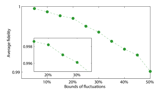
Figure 5: Average fidelity versus the bound on the fluctuations $\Theta$ for two coupled phase qubits. Each $\theta_{j}$ ($j=1,2,3$) has a truncated Gaussian distribution in $[1-\Theta,1+\Theta]$, and we assume $\theta_{1}=\theta_{2}$. The initial state is $|\psi_{0}\rangle=\frac{1}{\sqrt{2}}(|g,g\rangle+|e,g\rangle)$ and the target state is $|\psi_{\text{target}}\rangle=\frac{1}{\sqrt{2}}(|g,g\rangle+|e,e\rangle)$. Each average fidelity is calculated using 5000 samples.

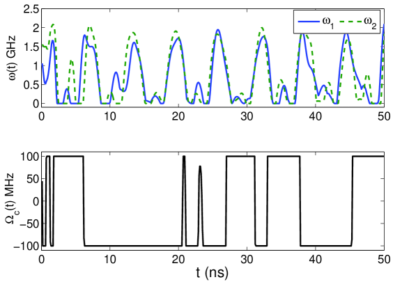
Figure 6: A set of “smart” fields corresponding to $\omega_{1}(t)$, $\omega_{2}(t)$ and $\Omega_{c}(t)$ for the problem of two coupled phase qubits when the bound on the fluctuations is very large, with $\Theta=25\%$ (i.e., 50% fluctuations).

Discussion

In numerical examples, a small number of samples for each possible fluctuation parameter is used to construct an augmented system. It is possible to achieve improved performance by using more samples. However, an increase in the number of samples in the training step will consume more computation resources. The tradeoff between resource consumption and performance that can be achieved should be investigated for specific tasks. In the SLC method, we employ a general gradient-flow-based algorithm to learn “smart” fields and the algorithm is usually much more efficient than other stochastic search algorithms (e.g., genetic algorithms) for control design of quantum systems Rabitz-et-al-2004 . The “smart” fields are “optimal” to the control landscapes of different samples since they are found by simultaneously optimizing the fields for these samples. It may be possible to use a similar theory to the quantum control landscape theory developed in Rabitz-et-al-2004 to analyze these optimal properties. As examples, we only consider that each possible fluctuation parameter has several specific distributions in the testing step. However, the proposed method also works well for other time-varying or time-invariant distributions. Numerical results show that, in the training step, sampling fluctuation parameters according to simple uniform distributions can achieve excellent performance for these cases where the fluctuation parameters have other distributions. In our numerical examples, we only consider three classes of superconducting quantum systems with several specific parameter settings. Our method is also applicable to other superconducting qubits, such as the “Xmon” and “gmon” qubits Martinis-et-al-2013PRL ; Martinis-et-al-2014-1 ; Martinis-et-al-2014-2 , since its performance is insensitive to the parameter settings and possible fluctuations.

In conclusion, we use a sampling-based learning control method to design robust fields that are insensitive to possible fluctuations. Numerical results show that the method can efficiently find “smart” fields for superconducting qubits even in the presence of 40%$\sim$50% fluctuations in different parameters. The proposed method has potential for robust quantum information processing and can contribute to the design of more reliable quantum devices.

Methods

Sampling-based learning control (SLC). The SLC method was first proposed for the control design of inhomogeneous quantum ensembles Chen-et-al-2013arXiv . In this method, several artificial samples, generated through sampling possible inhomogeneous parameters, are used to learn optimal control fields and then these fields are applied to additional samples to test their performance. In this paper, we develop an SLC method for guiding the design of robust control fields for superconducting quantum systems with fluctuations.

Consider a quantum system with Hamiltonian $H(u,\theta,t)$ and the evolution of its state $|\psi(t)\rangle$ is described by the following Schrödinger equation:

$$i\hbar|{\dot{\psi}}(t)\rangle=H(u,\theta,t)|\psi(t)\rangle$$ (7)

where $u$ represents the control field and $\theta$ characterizes possible fluctuations. In the SLC method, we first generate $N$ artificial samples by selecting different values of $\theta$ (e.g., the $N$ samples correspond to $\theta^{(1)}$, $\theta^{(2)}$,$\cdots$, $\theta^{(N)}$). Using these samples, an augmented system is constructed as follows

$$i\hbar\left(\begin{array}[]{c}|{\dot{\psi}}_{\theta^{(1)}}(t)\rangle\\ |{\dot{\psi}}_{\theta^{(2)}}(t)\rangle\\ \vdots\\ |{\dot{\psi}}_{\theta^{(N)}}(t)\rangle\\ \end{array}\right)=\left(\begin{array}[]{c}H(u,\theta^{(1)},t)|\psi_{\theta^{(1)}}(t)\rangle\\ H(u,\theta^{(2)},t)|\psi_{\theta^{(2)}}(t)\rangle\\ \vdots\\ H(u,\theta^{(N)},t)|\psi_{\theta^{(N)}}(t)\rangle\\ \end{array}\right).$$ (8)

The performance function $J(u)$ for the augmented system is defined as

$$J(u):=\frac{1}{N}\sum_{n=1}^{N}J_{\theta^{(n)}}(u)=\frac{1}{N}\sum_{n=1}^{N}|\langle\psi_{\theta^{(n)}}(T)|\psi_{\text{target}}\rangle|^{2}$$ (9)

where $|\psi_{\text{target}}\rangle$ is the target state and $|\psi_{\theta^{(n)}}(T)\rangle$ is the final state for one sample (corresponding to $\theta^{(n)}$) at the time $T$. The task in the training step is to find an optimal control field $u^{*}$ that maximizes the performance function defined in Eq. (9).

In the testing step, we apply the optimized field $u^{*}$ to additional samples generated by randomly sampling the fluctuation parameters and evaluate the performance in terms of the fidelity. If the average fidelity for the tested samples are good enough, we accept the designed field and complete the design process. Otherwise, we should go back to the training step and learn another optimized control field (e.g., restarting the training step with a new initial field or a new set of samples).

Sampling. In order to construct an augmented system, we need to generate $N$ artificial samples. We assume that there are two fluctuation parameters $\theta^{x}$ and $\theta^{z}$. We may choose some equally-spaced samples in the $\theta^{x}$–$\theta^{z}$ space. For example, the intervals $[1-\Theta^{x},1+\Theta^{x}]$ and $[1-\Theta^{z},1+\Theta^{z}]$ are divided into $N_{x}+1$ and $N_{z}+1$ subintervals, respectively, where $N_{x}$ and $N_{z}$ are usually positive odd numbers. Then, the number of samples $N=N_{x}N_{z}$, where $\theta^{x}_{m}$ and $\theta^{z}_{n}$ can be chosen from the combination of $(\theta^{x}_{m},\theta^{z}_{n})$ as follows

$$\left\{\begin{array}[]{c}\theta^{x}_{m}\in\{\theta^{x}_{m}=1-\Theta^{x}+\frac{(2m-1)\Theta^{x}}{N_{x}},\ m=1,2,\ldots,N_{x}\},\\ \theta^{z}_{n}\in\{\theta^{z}_{n}=1-\Theta^{z}+\frac{(2n-1)\Theta^{z}}{N_{z}},\ \ n=1,2,\ldots,N_{z}\}.\\ \end{array}\right.$$ (10)

Gradient-flow-based learning algorithm. In order to find an optimal control field $u^{*}$ for the augmented system (8), a good choice is to follow the direction of the gradient of $J(u)$ as an ascent direction. Assume that the performance function is $J(u_{0})$ with an initial field $u_{0}$. We can apply the gradient flow method to approximate an optimal control field $u^{*}$. This can be achieved by iterative learning using the following updating (for details, see, e.g., Chen-et-al-2013arXiv )

$$u_{k+1}(t)=u_{k}(t)+\eta_{k}\nabla J(u_{k}),$$ (11)

where $\eta_{k}$ is the updating stepsize for the $k$th iteration and $\nabla J(u)$ denotes the gradient of $J(u)$ with respect to the control $u$. The calculation of $\nabla J(u)$ is described in Chen-et-al-2013arXiv ; Roslund-and-Rabitz-2009 . For practical implementations, we usually divide the time interval $[0,T]$ equally into a number of smaller time intervals $\Delta t$ and assume that the control fields are constant within each time interval $\Delta t$. In the algorithm, we assume $u(t)\in[V_{-},V_{+}]$. If $u_{k+1}\leq V_{-}$, we let $u_{k+1}=V_{-}$. If $u_{k+1}\geq V_{+}$, we let $u_{k+1}=V_{+}$. In numerical computations, if the change of the performance function for $100$ consecutive training steps is less than a small threshold $\epsilon$ (i.e., $|J(u_{k+100})-J(u_{k})|<\epsilon$ for some $k$), then the algorithm converges and we end the training step. In this paper, we let $\epsilon=10^{-4}$ for all numerical results.

Acknowledgments The work is supported by the Australian Research Council (DP130101658, FL110100020) and National Natural Science Foundation of China (Nos. 61273327 and 61374092). F.N. is partially supported by the RIKEN iTHES Project, MURI Center for Dynamic Magneto-Optics, and a Grant-in-Aid for Scientific Research (S).

Author contributions D.D., C.C., B.Q. and I.R.P. developed the scheme of robust sampling-based learning control, D.D. and F.N. designed the illustrative examples of superconducting quantum circuits. C.C. performed the numerical simulations. All authors discussed the results and contributed to the writing of the paper.

Additional information

Competing financial interests: The authors declare no competing financial interests.

References

- (1) You, J. Q. & Nori, F. Superconducting circuits and quantum information. Physics Today 58, 42-47 (2005).
- (2) Wendin, G. & Shumeiko, V. S. In Handbook of Theoretical and Computational Nanotechnology, edited by M. Rieth and W. Schommers (American Scientific Publishers, Karlsruhe, Germany, 2006), Chap. 12; arXiv:cond-mat/0508729
- (3) Schoelkopf, R. J. & Girvin, S. M. Wiring up quantum systems. Nature 451, 664-669 (2008).
- (4) Clarke, J. & Wilhelm, F. K. Superconducting quantum bits. Nature 453, 1031-1042 (2008).
- (5) You, J. Q. & Nori, F. Atomic physics and quantum optics using superconducting circuits. Nature 474, 589-597 (2011).
- (6) Xiang, Z. L., Ashhab, S., You, J. Q. & Nori, F. Hybrid quantum circuits: Superconducting circuits interacting with other quantum systems. Rev. Mod. Phys. 85, 623-653 (2013).
- (7) Georgescu, I., Ashhab, S. & Nori, F. Quantum Simulation. Rev. Mod. Phys. 86, 153-185 (2014).
- (8) Pashkin, Yu. A., et al. Quantum oscillations in two coupled charge qubits. Nature 421, 823-826 (2003).
- (9) Steffen, M., et al. High-coherence hybrid superconducting qubit. Phys. Rev. Lett. 105, 100502 (2010).
- (10) Chiorescu, I., et al. Coherent dynamics of a flux qubit coupled to a harmonic oscillator. Nature 431, 159-162 (2004).
- (11) Wallraff, A., et al. Strong coupling of a single photon to a superconducting qubit using circuit quantum electrodynamics. Nature 431, 162-167 (2004).
- (12) Wilson, C. M., et al. Observation of the dynamical Casimir effect in a superconducting circuit. Nature 479, 376-379 (2011).
- (13) Liu, Y. X., You, J. Q.,Wei, L. F., Sun, C. P. & Nori, F. Optical selection rules and phase-dependent adiabatic state control in a superconducting quantum circuit. Phys. Rev. Lett. 95, 087001 (2005).
- (14) Valenzuela, S.O., et al. Microwave-induced cooling of a superconducting qubit. Science 314, 1589-1592 (2006).
- (15) Sillanpää, M. A., Park, J. I. & Simmonds, R. W. Coherent quantum state storage and transfer between two phase qubits via a resonant cavity. Nature 449, 438-442 (2007).
- (16) Wei, L. F., Johansson, J. R., Cen, L. X., Ashhab, S. & Nori, F. Controllable coherent population transfers in superconducting qubits for quantum computing. Phys. Rev. Lett. 100, 113601 (2008).
- (17) Steffen, M., et al. Measurement of the entanglement of two superconducting qubits via state tomography. Science 313, 1423-1425 (2006).
- (18) Hofheinz, M., et al. Synthesizing arbitrary quantum states in a superconducting resonator. Nature 459, 546-549 (2009).
- (19) McDermott, R. Materials orignins of decoherence in superconducting qubits. IEEE Trans. Appl. Superconductivity. 19, 2-13 (2009).
- (20) Valente, D. C. B., Mucciolo, E. R. & Wilhelm, F. K. Decoherence by electromagnetic fluctuations in double-quantum-dot charge qubits. Phys. Rev. B, 82, 125302 (2010).
- (21) Vijay, R., et al. Stabilizing Rabi oscillations in a superconducting qubit using quantum feedback. Nature 490, 77-80 (2012).
- (22) Murch, K. W., Weber, S. J., Levenson-Falk, E. M., Vijay, R. & Siddiqi, I. noise of Josephson-junction-embedded microwave resonators at single photon energies and millikelvin temperatures. Appl. Phys. Lett. 100, 142601 (2012).
- (23) Slichter, D. H., et al. Measurement-induced qubit state mixing in circuit QED from up-converted dephasing noise. Phys. Rev. Lett. 109, 153601 (2012).
- (24) Khani, B., Merkel, S. T., Motzoi, F., Gambetta, J. M. & Wilhelm, F. K. High-fidelity quantum gates in the presence of dispersion. Phys. Rev. A 85, 022306 (2012).
- (25) Paladino, E., Galperin, Y. M., Falci, G. & Altshuler, B. L. noise: Implications for solid-state quantum information. Rev. Mod. Phys. 86, 361-418 (2014).
- (26) Pravia, M. A., et al. Robust control of quantum information. J. Chem. Phys. 119, 9993-10001 (2003)
- (27) Falci, G., D’Arrigo, A., Mastellone, A. & Paladino, E. Initial decoherence in solid state qubits. Phys. Rev. Lett. 94, 167002 (2005).
- (28) Montangero, S., Calarco, T. & Fazio, R. Robust optimal quantum gates for Josephson charge qubits. Phys. Rev. Lett. 99, 170501 (2007).
- (29) Zhang, J., Liu, Y. X. & Nori, F. Cooling and squeezing the fluctuations of a nanomechanical beam by indirect quantum feedback control. Phys. Rev. A 79, 052102 (2009).
- (30) Zhang, J., Greenman, L., Deng, X. & Whaley, K. B. Robust control pulses design for electron shuttling in solid state devices. IEEE Trans. Control Syst. Technology 22, 2354-2359 (2014).
- (31) Wu, R. B., et al. Spectral analysis and identification of noises in quantum systems. Phys. Rev. A 87, 022324 (2013).
- (32) Kosut, R. L., Grace, M. D. & Brif, C. Robust control of quantum gates via sequential convex programming. Phys. Rev. A 88, 052326 (2013).
- (33) James, M. R., Nurdin, H. I. & Petersen, I. R. control of linear quantum stochastic systems. IEEE Trans. Automat. Control 53, 1787-1803 (2008).
- (34) Dong D. & Petersen, I. R. Sliding mode control of quantum systems. New J. Phys. 11, 105033 (2009).
- (35) Wiseman H. M. & Milburn, G. J. Quantum Measurement and Control (Cambridge University Press, Cambridge, England, 2010).
- (36) Gaitan, F. Quantum Error Correction and Fault Tolerant Quantum Computing (CRC Press, Boca Raton, Florida, USA, 2008).
- (37) Viola, L., Knill, E. & Lloyd, S. Dynamical decoupling of open quantum systems. Phys. Rev. Lett. 82, 2417-2421 (1999).
- (38) Khodjasteh, K., Lidar, D. A. & Viola, L. Arbitrarily accurate dynamical control in open quantum systems. Phys. Rev. Lett. 104, 090501 (2010).
- (39) Rabitz, H., Hsieh, M. M. & Rosenthat, C. M. Quantum optimally controlled transition landscapes. Science 303, 1998-2001 (2004).
- (40) Spörl, A. K., et al. Optimal control of coupled Josephson qubits. Phys. Rev. A 75, 012302 (2007).
- (41) Ginossar, E., Bishop, Lev S., Schuster, D. I. & Girvin, S. M. Protocol for high-fidelity readout in the photon-blockade regime of circuit QED. Phys. Rev. A 82, 022335 (2010).
- (42) Motzoi, F., Gambetta, J. M., Merkel, S. T. & Wilhelm, F. K. Optimal control methods for rapidly time-varying Hamiltonians. Phys. Rev. A 84, 022307 (2011).
- (43) Egger, D. J. & Wilhelm, F. K. Adaptive hybrid optimal quantum control for imprecisely characterized systems. Phys. Rev. Lett. 112, 240503 (2014).
- (44) Chen, C., Dong, D., Long, R., Petersen, I. R. & Rabitz, H. Sampling-based learning control of inhomogeneous quantum ensembles. Phys. Rev. A 89, 023402 (2014).
- (45) Bialczak, R. C., et al. Fast tunable coupler for superconducting qubits. Phys. Rev. Lett. 106, 060501 (2011).
- (46) Pinto, R. A., Korotkov, A. N., Geller, M. R., Shumeiko, V. S. & Martinis, J. M. Analysis of a tunable coupler for superconducting phase qubits. Phys. Rev. A 82, 104522 (2010).
- (47) Barends, R., et al. Coherent Josephson qubit suitable for scalable quantum integrated circuits. Phys. Rev. Lett. 111, 080502 (2013).
- (48) Chen, Y., et al. Qubit architecture with high coherence and fast tunable coupling. arXiv:1402.7367, quant-ph (2014).
- (49) Geller, M. R., et al. Tunable coupler for superconducting Xmon qubits: Perturbative nonlinear model. arXiv:1405.1915, quant-ph (2014).
- (50) Nielsen, M. A. & Chuang, I. L. Quantum Computation and Quantum Information (Cambridge University Press, Cambridge, England, 2010).
- (51) You, J. Q., Tsai, J. S. & Nori, F. Controllable manipulation and entanglement of macroscopic quantum states in coupled charge qubits. Phys. Rev. B 68, 024510 (2003).
-
(52)
Roslund, J. & Rabitz, H. Gradient algorithm applied to
laboratory quantum control. Phys. Rev. A 79,
053417 (2009).