A complete data frame work for fitting power law distributions

Abstract

Over the last few decades power law distributions have been suggested as forming generative mechanisms in a variety of disparate fields, such as, astrophysics, criminology and database curation. However, fitting these heavy tailed distributions requires care, especially since the power law behaviour may only be present in the distributional tail. Current state of the art methods for fitting these models rely on estimating the cut-off parameter $x_{\min}$. This results in the majority of collected data being discarded. This paper provides an alternative, principled approached for fitting heavy tailed distributions. By directly modelling the deviation from the power law distribution, we can fit and compare a variety of competing models in a single unified framework.

1 Introduction

Power law probability distributions have the relatively simple form of

$$p(x)\propto x^{-\alpha}$$ (1)

where $\alpha>1$ and $x>0$. The parameter $\alpha$, is often referred to as the exponent or scaling parameter. Although straightforward, these distributions have gathered scientific interest from many areas, including terrorism, astrophysics, neuroscience, biology, database curation and criminology[7, 14, 1, 22, 2, 10].

This apparent ubiquity of power laws in a wide range of disciplines was questioned by Stumpf and Porter[19]. The authors’ point out that many “observed” power law relationships are highly suspect. In particular, estimating the power law exponent on a log-log plot, whilst appealing, is a very poor technique for fitting these types of models. Instead, a systematic, principled and statistical rigorous approach should be applied.

Power law distributions are often described as “scale-free” - indicating that common, small events are qualitatively similar to large, rare events. Identifying a power law can highlight the presence of underlying generative mechanism of interest.

Determining whether a quantity follows a power law distribution is complicated by the large fluctuations in the tail of the empirical distribution. These large spikes follow naturally from the power law distribution. For the continuous power law distribution, the raw moments are

$$E[X^{m}]=\int_{x_{\min}}^{\infty}x^{m}p(x)\,dx=\frac{\alpha-1}{\alpha-1-m}x_{\min}^{m}\;.$$

So when

• $1<\alpha\leq 2$, all moments diverge, i.e. $E[X]=\infty$;

• $2<\alpha\leq 3$, all second and higher-order moments diverge, i.e. $E[X^{2}]=\infty$;

• $3<\alpha\leq m+1$, all $m^{\text{th}}$ and higher-order moments diverge, i.e. $E[X^{m}]=\infty$.

However, large outlying values in the tail of the distribution are not unique to power laws. Many other “standard” distributions, such as the log normal, are characterised with heavy tails.

A further complication, is that the power law distribution may only be appropriate in the distributional tail, i.e. power law patterns only occur when $x\geq x_{\min}$. While the value of the $x_{\min}$ cut-off could be estimated by eye using log-log plots, this would obviously be a poor inference technique.

Clauset et al, 2009 introduced a principled set of methods for fitting and testing power law distributions[6]. Their approach is straightforward and appealing. They couple a distance-based test for estimating $x_{\min}$, with a standard maximum likelihood technique for inferring $\alpha$. Competing models can be compared using a likelihood ratio test[21]. However, their method does have three main draw-backs. First, by fitting $x_{\min}$ we are discarding all data below that cut-off. Second, it is unclear how to compare distributions where each distribution has a different $x_{\min}$. Third, although it is possible to make predictions in the tail of the distribution[9], making future predictions over the entire data space is not possible since values less than $x_{\min}$ have not been directly modelled.

In a recent paper, Peterson et al. 2013, propose a generative mechanism that describes the formation of heavy tailed distributions[16]. This neat formulation uses a statistical physics framework to express the underlying model in terms of shared costs and economies of scale. While this formulation fits the entire data set, some of the fits in the tail of the distributions were not optimal (in particular, the Github and Petster data sets shown in figure 1a).

Estimating $x_{\min}$ directly can impose a strange dichotomy between relevant and irrelevant observations. Instead, we adopt a different approach. Rather than directly estimating $x_{\min}$ and thereby discarding data, we model the entire data set as the deviation away from a power law (or other heavy tailed) distribution. By modelling the entire dataset, a number of standard statistical techniques, which are not straightforward in other power law modelling frameworks, become amenable. For example,

• prediction of future values of the phenomena of interest (see section 3.1);

• comparing different distributions models using AIC and BIC (see section 3.2);

• investigating model fit (see sections 3, 3.1 and 3.2);

• comparing different datasets (see section 3.1).

2 Method

In this paper we propose to model heavy tailed distributions using the distribution

$$f(x;\mbox{\boldmath$\theta$},\mbox{\boldmath$\phi$}) =Pr(X=x)$$

$$=\frac{g(x;\mbox{\boldmath$\theta$})\times D(x;\mbox{\boldmath$\phi$})}{C(\mbox{\boldmath$\theta$},\mbox{\boldmath$\phi$})}\quad\text{for}\quad x=1,\ldots$$ (2)

where $(\mbox{\boldmath$\theta$},\mbox{\boldmath$\phi$})$ are model parameters and $C(\mbox{\boldmath$\theta$},\mbox{\boldmath$\phi$})$ is a normalising constant. The function $f(\cdot)$ consists of two key components.

• A heavy-tailed distribution: $g(x;\mbox{\boldmath$\theta$})$. This could be, for example, a power law, log normal or other heavy tailed distribution. Typically, this function would fit the tail of the distribution well.

• A difference function: $D(x;\mbox{\boldmath$\phi$})$. This function describes the deviation between the heavy tailed distribution, $g(x;\mbox{\boldmath$\theta$})$ and the data. The key properties are $D(x;\mbox{\boldmath$\phi$})>0$ and as $x\rightarrow\infty$, $D(x;\mbox{\boldmath$\phi$})\rightarrow 1$.

Typical functional forms for $D(x;\mbox{\boldmath$\phi$})$ are

$$D(x;\mbox{\boldmath$\phi$})=1-e^{-(\phi_{0}+\phi_{1}(x-1))}\quad\text{Unit exponential CDF}$$

and

$$D(x;\mbox{\boldmath$\phi$})=\frac{1}{1+e^{-(\phi_{0}+\phi_{1}(x-1))}}\quad\text{Inverse logistic function.}$$

To fit model (2) we follow the Bayesian paradigm. Let $\pi(\mbox{\boldmath$\theta$})$ and $\pi(\mbox{\boldmath$\phi$})$ denote the respective prior densities for $\theta$ and $\phi$, and $\mathcal{D}$ is the observed data. Fully Bayesian inference can then proceed by sampling

$$\pi(\mbox{\boldmath$\theta$},\mbox{\boldmath$\phi$}\,|\,\mathcal{D})\propto\pi(\mbox{\boldmath$\theta$})\pi(\mbox{\boldmath$\phi$})f(\mathcal{D}\,|\,\mbox{\boldmath$\theta$},\mbox{\boldmath$\phi$})\;,$$ (3)

using a Markov chain Monte Carlo algorithm. To explore the parameter space, a multivariate Gaussian random walk proposal can be used, with the tuning parameter obtained from pilot runs.

2.1 Parameter estimation

Inferences regarding the parameters of $g(x;\mathbf{\mbox{\boldmath$\theta$}})$, e.g. the power law scaling parameter, are obtained from $\pi(\mbox{\boldmath$\theta$},\mbox{\boldmath$\phi$}\,|\,\mathcal{D})$. Intuitively, the cut-off parameter $x_{\min}$ corresponds to when $D(x;\mbox{\boldmath$\phi$})\simeq 1$. So a marginal posterior density for $x_{\min}$ can be obtained by calculating

$$\arg\min_{x}D(x;\mbox{\boldmath$\phi$})>\alpha\;,$$ (4)

where $\phi$ are posterior samples and $\alpha$ is a threshold.

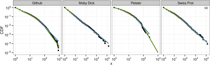
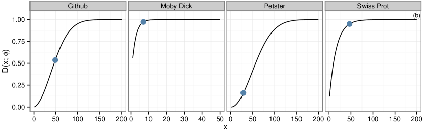
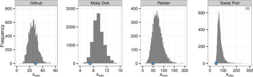
Figure 1: (a) Empirical distributions for the four example data sets. The green is the fitted function $f(x;\theta,\mbox{\boldmath$\phi$})$. The blue line is a fitted power law function, with parameters estimated using the CSN method. (b) A plot of the difference function $D(x;\mbox{\boldmath$\phi$})$ (where $\phi$ has been set to their posterior mean values). The blue dots shows the estimated value of $x_{\min}$ using the CSN method. (c) Estimated values of $x_{\min}$, obtained via $\arg\min_{x}D(x;\mbox{\boldmath$\phi$})>0.95$.

3 Examples

Figure 1 gives four illustrative examples.

• Project membership on the social coding web site GitHub[5].

• Occurrences of unique words in the novel Moby Dick[15].

• Friendships between users of the Petster social networking site Hamsterster[13].

• Occurrences of words in the Swiss-Prot database[2].

Each of the distributions in figure 1a has a “long-tail”. However, the distributional shapes differ. The word occurrence data sets - Moby Dick and Swiss Prot - have long power law like distributions. Whereas the social networking data sets - Petster and Github - have a more curved distribution.

In each example $g(x;\mbox{\boldmath$\theta$})$ is a power law distribution (with $x_{\min}=1$), i.e.

$$g(x,\theta)=\frac{x^{-\theta}}{\zeta(\theta)}\quad\text{for}\quad x=1,\ldots$$ (5)

where $\theta$ is the power law scaling parameter and

$$\zeta(\theta)=\sum_{i=1}^{\infty}\frac{1}{i^{\theta}}$$

is Riemann zeta function. To model the deviation away from the power law distribution, we use the unit exponential cumulative density function

$$D(x;\mbox{\boldmath$\phi$})=1-e^{-\phi_{0}-\phi_{1}(x-1)-\phi_{2}(x-1)^{2}}$$ (6)

where $\mbox{\boldmath$\phi$}=\{\phi_{0},\phi_{1},\phi_{2}\}\geq 0$. So $D(x=1;\mbox{\boldmath$\phi$})=1-e^{-\phi_{0}}$ and $g(x=\infty;\mbox{\boldmath$\phi$})=1$.

Figure 1a gives the empirical CDF of each data set and the fitted function $f(x;\theta,\mbox{\boldmath$\phi$})$. Also shown is a fitted power law distribution where $x_{\min}$ and the scaling parameter $\theta$ were estimated using the CSN method from Clauset et al.[6]. Figure 1b plots the difference function $D(x;\mbox{\boldmath$\phi$})$ along with the estimated $x_{\min}$ value obtained from the CSN method.

For each data set in figure 1a, $f(x;\theta,\mbox{\boldmath$\phi$})$ provides an excellent fit. However, the key benefit is that all data is used (see table 1 for an exact breakdown). For example, in the Moby Dick data set since $x_{\min}=7$, fitting a power law using CSN would result in discarding around 84% of the collected data.

For the network data sets, the standard power law fit is relatively poor, however, our flexible formulation still provides an excellent fit.

Inference can also be made about plausible values $x_{\min}$ by calculating

$$\arg\min_{x}D(x;\mbox{\boldmath$\phi$})>0.95\;,$$

where $\phi$ are samples from the posterior. The results given in figure 1 are broadly consistent with the CSN method. However, the difference method also provides credible regions to assess parameter uncertainty.

Table 1: Summary statistics from model fits relating to figure 1. The values of $\hat{x}_{\text{min}}$ and $\hat{\alpha}$ were obtained CSN method. The parameter $\bar{\theta}$ is the average posterior value of $\theta$ in expression 5. The column, % $<\hat{x}_{\text{min}}$, gives the proportion of data that are less the $\hat{x}_{\text{min}}$.

Data set	$\hat{x}_{\text{min}}$	% $<\hat{x}_{\text{min}}$	$\hat{\alpha}$	$\bar{\theta}$
Github	49	97	2.74	3.21
Moby Dick	7	84	1.95	1.95
Petster	29	93	2.90	3.80
Swiss Prot	47	95	2.07	2.07

3.1 Data set comparison

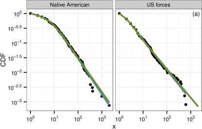
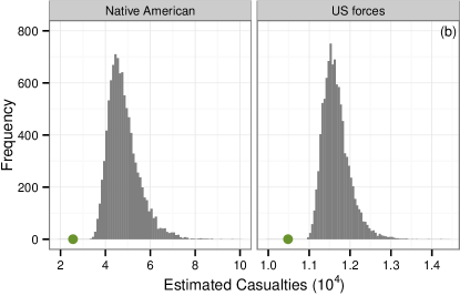
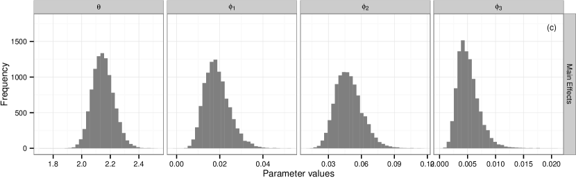
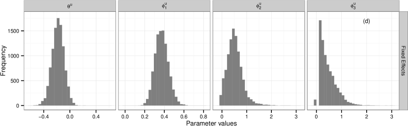
Figure 2: Casualty rates from the American Indian Wars. (a) Empirical CDFs with lines of best fit. Each data point represents the number of casualties at a recorded battle. The blue line is the fitted distribution obtained from the CSN method. The green line is the difference method.(b) The inferred total number of casualties. The green dot shows the observed number of casualties. (c) & (d) Posterior distributions for the parameters in $D(x;\cdot)$.

Recently Friedman investigated casualty rates in the American Indian Wars, 1776 to 1890[11]. Casualty rates are often controversial, since any estimation will involve inferences about missing data. It has been observed that many violent events, ranging from homicides to world wars, follow a power law distribution. For example, power laws have been used to characterise terrorist attacks[8], inter-state wars[4] and insurgent attacks[3]. Friedman uses this power law insight to fit distributions to the American Indian conflict, then infer missing casualties.

The casualty numbers for the Native American and US forces are shown in figure 2a. The Native American casualties were modelled using

$$g(x;\theta) =\frac{x^{-\theta}}{\zeta(\theta)}$$

$$h(x;\mbox{\boldmath$\phi$}) =1-e^{-\phi_{0}-\phi_{1}(x-1)-\phi_{2}(x-1)^{2}}$$

and the US forces casualties as

$$g_{U}(x;\theta^{*}) =\frac{x^{-\theta^{*}}}{\zeta(\theta^{*})}$$

$$h_{U}(x;\mbox{\boldmath$\phi$}^{*}) =1-e^{-\phi_{0}^{*}-\phi_{1}^{*}(x-1)-\phi_{2}^{*}(x-1)^{2}}$$

where

$$\theta^{*}=\theta+\theta^{u}\quad\text{and}\quad\phi_{i}^{*}=\phi_{i}+\phi_{i}^{u}\;.$$

Hence the parameters $\theta^{u}$ and $\mbox{\boldmath$\phi$}^{u}$ directly model the difference between the US forces and Native American casualties. The green line in figure 2a gives fitted function and blue line gives the standard power law fit using CSN method.

Assuming that the true underlying distribution is a power law, then the function $D(x;\mbox{\boldmath$\phi$})$ describes the number of missing casualties in the data. To infer the total number of casualties, we integrate the posterior over the uncertainty associated with the parameter. In other words, this predictive distribution is taken to be the posterior average of realisations from $g(x;\theta)$ and $g_{U}(x;\theta^{*})$. This integration yields figure 2b. The predictions given in figure 2b are consistent with Friedman’s analysis.

An additional benefit of fitting models in this way, is that it is straightforward to compare data sets. In this example, Figure 2c and 2d give the posterior distribution for the parameters. In general, the posterior of $\theta^{u}$ is negative, indicating that the causality rate is lower for US forces. Furthermore, since $D(x;\mbox{\boldmath$\phi$}+\mbox{\boldmath$\phi$}^{u})\geq D(x;\mbox{\boldmath$\phi$}^{u})$ the reporting of US force casualties was more consistent. Again, this agrees with the observations of Friedman.

3.2 Model comparison

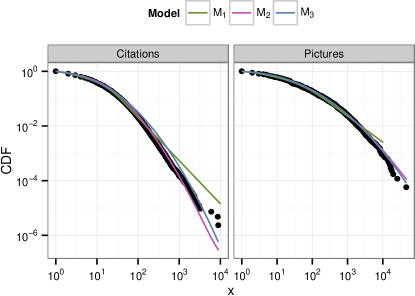
Figure 3: Citation and pictures data sets (details given in the text). The empirical CDF is given along with lines of best fit for models (i) $M_{1}$ - power law with unit exponential difference function. (ii) $M_{2}$ - discrete log normal with unit exponential difference function. (iii) $M_{3}$ - discrete log normal.

By fitting models to the entire data set, existing model comparison techniques can be leveraged. Figure 3 show two data sets.

• The number of citations received between publication and June 1997 by scientific papers published in 1981 and listed in the Science Citation Index[18];

• The connections in the bipartite picture tagging network of vi.sualize.us.[13].

For each data set we fitted three models.

1. $M_{1}$: where the deviation from a power law was modelled using a unit exponential function, i.e. expressions 5 and 6.

2. $M_{2}$: where the deviation from a discrete log normal was modelled using a unit exponential function.

3. $M_{3}$: a discrete log normal distribution.

Figure 3 show that the log normal based models, $M_{2}$ and $M_{3}$, fit the data set reasonably well. To formally compare models, we calculated the Bayesian Information Criterion (BIC) using the posterior means (see table 2). In both examples, the power law model was rejected when compared to log normal based models.

Table 2: Bayesian information criterion (BIC) values for competing model in the citation and pictures data set shown in figure 3. The smallest BIC value for each model is shown in bold.

	Model
Data set	$M_{1}$	$M_{2}$	$M_{3}$
Citations	$2,919,701$	$\mathbf{2,917,967}$	$2,921,903$
Pictures	$\phantom{2,}167,641$	$\phantom{2,}167,513$	$\mathbf{\phantom{2,}167,490}$

4 Discussion

Typically, researchers suggest that the power law feature is only present in the distributional tail. By modelling the deviation away from the power law (or other heavy tailed distribution), we have created a flexible and general framework. We reiterate that by modelling the entire data set, we circumvent the problem of estimating $x_{\min}$, and thereby discarding part of the data. Since we have avoided the $x_{\min}$ issue, standard statistical tools automatically become available.

By adopting a Bayesian framework, more complex observed data structures can be incorporated. For example, Virkar and Clauset recently consider “binned” data sets[20]. This relates to a number of data sets where the observations have been rounded. In the framework proposed in this paper, we could simply introduce an appropriate data error model, and integrate out the uncertainty using Markov chain Monte Carlo and the analysis would proceed as before.

Computing details

All simulations were performed on a machine with 4GB of RAM and with an Intel quad-core CPU using R[17]. The CSN power law fits were obtained using the poweRlaw package[12]. All code associated with this paper can be obtained from

https://github.com/csgillespie/plmcmc

References

- [1] J. M. Beggs and D Plenz. Neuronal avalanches in neocortical circuits. The Journal of Neuroscience, 23(35):11167–77, 2003.
- [2] M. J. Bell, C. S. Gillespie, D. Swan, and P. Lord. An approach to describing and analysing bulk biological annotation quality: a case study using UniProtKB. Bioinformatics, 28(18):i562–i568, 2012.
- [3] J. C. Bohorquez, S Gourley, A R Dixon, M Spagat, and N. F. Johnson. Common ecology quantifies human insurgency. Nature, 462(7275):911–4, 2009.
- [4] L. E. Cederman. Modeling the size of wars: from billiard balls to sandpiles. American Political Science Review, 97(1):135–150, 2003.
- [5] S. Chacon. The 2009 Github Contest. https://github.com/blog/466-the-2009-github-contest, 2009.
- [6] A. Clauset, C. R. Shalizi, and M. E. J. Newman. Power-law distributions in empirical data. SIAM Review, 51(4):661–703, 2009.
- [7] A. Clauset, M. Young, and K. S. Gleditsch. On the Frequency of Severe Terrorist Events. Journal of Conflict Resolution, 51(1):58–87, February 2007.
- [8] A. Clauset, M. Young, and K. S. Gleditsch. On the frequency of severe terrorist events. Journal of Conflict Resolution, 51(1):58–87, 2007.
- [9] Aaron Clauset and Ryan Woodard. Estimating the historical and future probabilities of large terrorist events. The Annals of Applied Statistics, 7(4):1838–1865, December 2013.
- [10] P. A. C. Duijn, V. Kashirin, and P. M. A. Sloot. The relative ineffectiveness of criminal network disruption. Scientific Reports, 4:4238, 2014.
- [11] J. A. Friedman. Using power laws to estimate conflict size. Journal of Conflict Resolution, April 2014.
- [12] C. S. Gillespie. Fitting heavy tailed distributions: the poweRlaw package. arXiv, 1407.3492, July 2014.
- [13] J. Kunegis. KONECT: the Koblenz network collection. In Proceedings of the 22nd international conference on World Wide Web companion, pages 1343–1350. International World Wide Web Conferences Steering Committee, 2013.
- [14] M. Michel, H. Kirk, and P. C. Myers. Mass distributions of stars and cores in young groups and clusters. The Astrophysical Journal, 735(1):51, 2011.
- [15] M. E. J. Newman. Power laws, Pareto distributions and Zipf’s law. Contemporary Physics, 46(5):323–351, 2005.
- [16] J. Peterson, P. D. Dixit, and K. A. Dill. A maximum entropy framework for nonexponential distributions. Proceedings of the National Academy of Sciences of the United States of America, 110(51):20380–5, 2013.
- [17] R Core Team. R: A Language and Environment for Statistical Computing. R Foundation for Statistical Computing, Vienna, Austria, 2013.
- [18] S Redner. How popular is your paper? An empirical study of the citation distribution. The European Physical Journal B-Condensed Matter and Complex Systems, 134:131–134, 1998.
- [19] M. P. H. Stumpf and M. A. Porter. Mathematics. Critical truths about power laws. Science, 335(6069):665–6, 2012.
- [20] Y. Virkar and A. Clauset. Power-law distributions in binned empirical data. The Annals of Applied Statistics, 8(1):89–119, 2014.
- [21] Q. H. Vuong. Likelihood ratio tests for model selection and non-nested hypotheses. Econometrica, 57:307–333, 1989.
- [22] H. Yu, P. Braun, M. A. Yildirim, I. Lemmens, K. Venkatesan, J. Sahalie, T. Hirozane-Kishikawa, F. Gebreab, N. Li, N. Simonis, T. Hao, J.-F. Rual, A. Dricot, A. Vazquez, R. R. Murray, C. Simon, L. Tardivo, S. Tam, N. Svrzikapa, C. Fan, A.-S. de Smet, A. Motyl, M. E. Hudson, J. Park, X. Xin, M. E. Cusick, T. Moore, C. Boone, M. Snyder, F. P. Roth, A.-L. Barabási, J. Tavernier, D. E. Hill, and M. Vidal. High-quality binary protein interaction map of the yeast interactome network. Science, 322(5898):104–10, 2008.