Three-Slit Ghost Interference and Nonlocal Duality

Abstract

A three-slit ghost interference experiment with entangled photons is theoretically analyzed using wave-packet dynamics. A nonlocal duality relation is derived which connects the path distinguishability of one photon to the interference visibility of the other.

I Introduction

Quantum entanglement and nonlocality are two aspects of correlations which are intimately related to each othernielson . Such fundamental aspects of quantum theory are extensively studiedhorodecki and today also its an emerging field of research. The correlated properties of entangled two-photon states have attracted attentions, due to their extensive applications in quantum optics and quantum informationstreak ; arthur . As a result, Strekalov et.al demonstrated the ghost interference experimentghostexp , which show a nonlocal behaviour with spontaneous parametric down-conversion(SPDC)kly source S, a common method of producing entangled photons, conventionally called signal and idler beamkwait ; imaging ; walborn , are then split by a polarized beam splitter into two beams, detected in coincidence by two distant pointlike photon detectors $D_{1}$ and $D_{2}$.

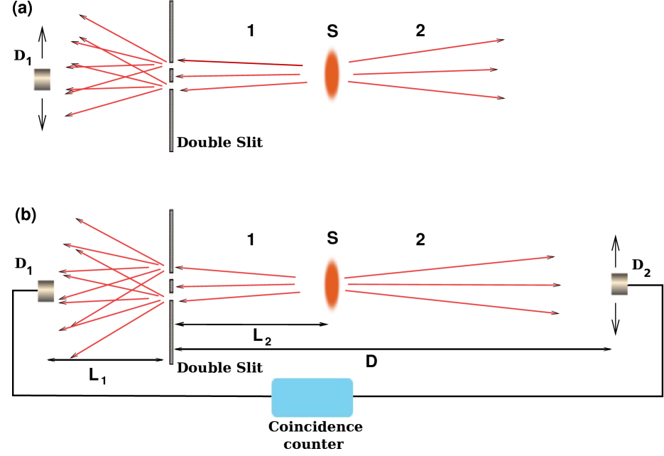
Figure 1: Schematic diagram of the two-slit ghost interference experiment.

A double-slit is in the path of photon 1, and the detector $D_{1}$ is kept behind (see FIG. 1(a)), no interference pattern is observed for photon 1, surprisingly, as one would normally expect Young’s double-slit interference. Also when the photon 2 is detected by $D_{2}$, in coincidence with a fixed detector $D_{1}$, the double-slit interference pattern is observed (see FIG. 1(b)), even though there is no double-slit in the path of photon 2. Many interesting outcomes are due to the spatial correlations which is with twin photons, produced in parametric down-conversionwal .

The two slit experiment has also been studied extensively in context of wave-particle duality and Bohr’s principle of complementarity . The fact that the wave and particle nature cannot be observed at the same time, is so fundamental that Bohr gave the principle, known as, the principle of complementaritybohr . Bohr stressed that the wave nature of particle, characterized by interference, and the particle nature, characterized by which way (i.e., which path) information, are mutually exclusive. A further question investigation was if the two natures could be observed simultaneously, and to what level of accuracy. A bound on simultaneous path distinguishability and fringe visibility is described by the so-called Englert-Greenberger-Yasin (EGY) relationgreen ; englert . The EGY duality relation is local, in the sense that when we talk of which-path distinguishability, we talk of the which-path knowledge of the same particle giving interference pattern. A nonlocal duality relation was derived for two slit experimenttabish , which relates the which-path information of one particle to the fringe visibility of the other.

At present the search for an analogous form of duality relation for multi slit experiments has generated quite a lot of research activity. Several attempts have been made to explore it quantativelydurr ; luis ; bim ; jak ; eng ; zaw . The simplest multi slit case is the three slit case, recently, a duality relation for three slit interference has been formulated asad , a step towards the search for an analogous form of duality relation for more than two slits. The analysis for four or multi slit interference is much more involved than that for two or three slit experiments, there it would be difficult to find phases for which extreme intensities occur, and thus the visibility.

Of late, a focussed interest has been generated towards the three-slit experimentsasad ; zel ; zaw ; urbasi ; ste ; udu ; hess ; nies ; sawan ; gag ; guti ; gutie . Three-slits are also used in generating qutrit states, their applications include implementation of quantum gameskole and in quantum tomographytagu ; pime .

In this paper, we propose and theoretically analyze a three-slit ghost interference experiment performed with entangled particles. Also a nonlocal duality relation is derived which connects the path distinguishability of one particle to the interference visibility of the other. Our analysis is general enough to describe any two entangled particles. It equally well applies to entangled photons, whether generated by SPDC or any other method like four-wave mixing.

II Three Slit Ghost Interference

In our proposed experiment, the two slits are replaced by three slits, in the earlier setup (see FIG. 2). The entangled photons 1 and 2 from the source S show an interference pattern, similar to the pattern observed from three slits experiment. Even though photon 2 never passes through the region between the source S and three slits, we see an interference pattern for photon 2, as if a beam of photon 2 with a source located at the position of detector $D_{1}$, get split by three-slits. This behavior can be qualitatively understood with the help of an advanced wave picture introduced by Klyshkoklyshko . In this picture, the detector $D_{1}$ plays the role of a source, which sends photon back towards the crystal. These photons are then reflected by the crystal as by mirror, compels them to follow the path of the signal photons, detected by the detector $D_{2}$. In this way, the increase in spatial filtering of the detector $D_{1}$, reduces the size of the source in the advanced wave picture, which increases the spatial coherence. In the following we do a more quantitative analysis.

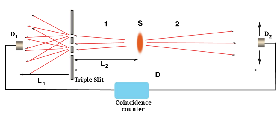
Figure 2: Schematic diagram of the three-slit ghost interference experiment.

III Wave-Packet Analysis

Our view is that the ghost interferencetqpcs is a result of position and momentum entanglement in photon pairs. Same phenomenon should be observed for any two entangled particles. SPDC is just one method of producing entangled particles. We will base our analysis on entangled pairs of particles. In order to theoretically analyze the entangled photons, a generalized EPR statetqajp is used, which unlike the EPR stateepr , is well behaved and fully normalized.

$$\Psi(z_{1},z_{2})=C_{1}\!\int_{-\infty}^{\infty}dp~{}e^{-p^{2}/4\hbar^{2}\sigma^{2}}~{}e^{-ipz_{2}/\hbar}~{}e^{ipz_{1}/\hbar}~{}e^{-{(z_{1}+z_{2})^{2}\over 4\Omega^{2}}},$$ (1)

where $C_{1}$ is a normalization constant, and $\sigma,\Omega$ are certain parameters whose physical significance will become clear in the following. In the limit $\sigma,\Omega\to\infty$ the state (1) reduces to the EPR state.

The pair of photons are assumed to travel in opposite directions along the x-axis, and the entanglement is in the z-direction. We will ignore the dynamics along the x-axis as it does not affect the entanglement. We assume that during the evolution for time $t$, the photon travels a distance equal to $ct$. Integration performed over $p$ in Eq.(1) gives:

$$\Psi(z_{1},z_{2})=\sqrt{{\sigma\over\pi\Omega}}~{}e^{-(z_{1}-z_{2})^{2}\sigma^{2}}e^{-(z_{1}+z_{2})^{2}/4\Omega^{2}}.$$ (2)

The uncertainty in positions and the wave-vector of two photons, along the z-axis, is given by

$$\Delta z_{1} = \Delta z_{2}=\sqrt{\Omega^{2}+1/4\sigma^{2}},$$

$$\Delta k_{1z} = \Delta k_{2z}={1\over 2}\sqrt{\sigma^{2}+{1\over 4\Omega^{2}}}.$$ (3)

The above equation gives the position and momentum spread of the photons in the z-direction. The time evolution of wave-function is essentially dictated by time evolution of wave-packet.

If the wave-function of a single photon at time $t=0$ is $\psi(z,0)$, then the wave-function of photon, after time t will evolve as

$$\psi(z,t)={1\over 2\pi}\int_{-\infty}^{\infty}\exp(ik_{z}z-i\omega(k_{z})t)~{}\tilde{\psi}(k_{z},0)~{}dk_{z},$$ (4)

where $\tilde{\psi}(k_{z},0)$ is the Fourier transform of $\psi(z,0)$ with respect to $z$.

In the above equation, if $k_{z}=k_{0}$, then it would be monochromatic approximation. But we have applied an alternative approach. The photon approximately travels in the x-direction, but can slightly deviate in the z-direction, so it can pass through slits which are located at different z-positions, and therefore its true wave-vector will be given by,

$$\omega(k_{z})=c\sqrt{k_{x}^{2}+k_{z}^{2}}$$ (5)

Since the photon travel along x-axis, hence for $k_{x}\gg k_{z}$ , one can write $k_{x}\approx k_{0}$, where $k_{0}$ is the wave-number of the photon associated with its wavelength, $k_{0}=2\pi/\lambda$. The dispersion along z-axis can be approximated by

$$\omega(k_{z})\approx ck_{0}+ck_{z}^{2}/2k_{0}.$$ (6)

The above relation can also be obtained using paraxial approximation, for small angle $\theta$, with $k_{x}=k_{0}\cos\theta$, and $k_{z}=k_{0}\sin\theta$.

Using (6), the Eq.(4) becomes

$$\psi(z,t)={e^{-ick_{0}t}\over 2\pi}\int_{-\infty}^{\infty}\exp(ik_{z}z-ictk_{z}^{2}/2k_{0})~{}\tilde{\psi}(k_{z},0)~{}dk_{z}$$ (7)

In case of entangled photons, after time $t_{0}$, photon 1 reaches the triple slit ($ct_{0}=L_{2}$), and photon 2 travels a distance $L_{2}$ towards detector $D_{2}$. Therefore, the wave-function of the entangled photons after time $t_{0}$ is given by:

$$\Psi(z_{1},z_{2},t_{0}) = {e^{-2ick_{0}t_{0}}\over 4\pi^{2}}\int_{-\infty}^{\infty}dk_{1}\exp(ik_{1}z_{1}-ict_{0}k_{1}^{2}/2k_{0})$$

$$\times \int_{-\infty}^{\infty}dk_{2}\exp(ik_{2}z_{2}-ict_{0}k_{2}^{2}/2k_{0})~{}\tilde{\Psi}(k_{1},k_{2},0),$$

where $\tilde{\Psi}(k_{1},k_{2},0)$ is the Fourier transform of (2) with respect to $z_{1},z_{2}$.

To investigate the effect on the entangled state, one can use two different approaches. The first, most obvious is to model a potential for three-slits, and calculate its evolution in that potential. We will follow the second, a comparatively easier approach, here we capture the essence of the effect of triple slit on the wave-function, without going into tedious calculations. When the state interacts with a single-slit, we assume, that a Gaussian wave-packet emerges from that slit, centered at its location, whose width is related to the width of the slit.

Consider the state of particle 1 passing through the slits A, B and C be $|\phi_{A}\rangle$, $|\phi_{B}\rangle$ and $|\phi_{C}\rangle$, respectively. Some part of the state of particle 1 will be blocked, represented by $|\chi\rangle$. All these states are orthogonal, and the actual state of particle 1 can be expanded in this basis.

$$|\Psi(t_{0})\rangle = |\phi_{A}\rangle\langle\phi_{A}|\Psi\rangle+|\phi_{B}\rangle\langle\phi_{B}|\Psi\rangle$$ (9)

$$+ |\phi_{C}\rangle\langle\phi_{C}|\Psi\rangle+|\chi\rangle\langle\chi|\Psi\rangle.$$

The terms $\langle\phi_{A}|\Psi\rangle,~{}\langle\phi_{B}|\Psi\rangle,~{}\langle\phi_{C}|\Psi\rangle,~{}\langle\chi|\Psi\rangle$ are states of particle 2 and can be written explicitly as follows.

$$|\psi_{A}\rangle = \langle\phi_{A}|\Psi(t_{0})\rangle,$$

$$|\psi_{B}\rangle = \langle\phi_{B}|\Psi(t_{0})\rangle,$$

$$|\psi_{C}\rangle = \langle\phi_{C}|\Psi(t_{0})\rangle,$$

$$|\psi_{\chi}\rangle = \langle\chi|\Psi(t_{0})\rangle,$$ (10)

The entangled state after particle 1 passes through triple-slit will be given by:

$$|\Psi\rangle=|\phi_{A}\rangle|\psi_{A}\rangle+|\phi_{B}\rangle|\psi_{B}\rangle+|\phi_{C}\rangle|\psi_{C}\rangle+|\chi\rangle|\psi_{\chi}\rangle,$$ (11)

where $|\phi_{A}\rangle$ , $|\phi_{B}\rangle$ and $|\phi_{C}\rangle$ are states of particle 1, and $|\psi_{A}\rangle$ , $|\psi_{B}\rangle$ and $|\psi_{C}\rangle$ are states of particle 2. In general, even if $|\phi_{A}\rangle$, $|\phi_{B}\rangle$ and $|\phi_{C}\rangle$ are orthogonal, $|\psi_{A}\rangle$, $|\psi_{B}\rangle$ and $|\psi_{C}\rangle$ may or may not be orthogonal depending on the values of $\Omega$ and $\sigma$, which dictate the degree of correlation between two particles. Perfect correlation will happen only when $\sigma,\Omega\to\infty$ , in that case Eq.(1) becomes the idealized EPR state.

The first three term represents the amplitude of particle 1 passing through these slits, and the last term represents the amplitude of being blocked or reflected. The linearity of the Schrödinger equation assures that the first three terms and the last term evolve independently. Since the experiment consider only those photon 1 which passes through the triple slit, we can throw away the last term. This will not change anything except the renormalization of the state.

For simplicity, we assume that $\langle z_{1}|\phi_{A}\rangle$, $\langle z_{1}|\phi_{B}\rangle$, and $\langle z_{1}|\phi_{C}\rangle$ are Gaussian wave-packets:

$$\langle z_{1}|\phi_{A}\rangle=\phi_{A}(z_{1}) = {1\over(\pi/2)^{1/4}\sqrt{\epsilon}}e^{-(z_{1}-z_{0})^{2}/\epsilon^{2}},$$

$$\langle z_{1}|\phi_{B}\rangle=\phi_{B}(z_{1}) = {1\over(\pi/2)^{1/4}\sqrt{\epsilon}}e^{-z_{1}^{2}/\epsilon^{2}},$$

$$\langle z_{1}|\phi_{C}\rangle=\phi_{C}(z_{1}) = {1\over(\pi/2)^{1/4}\sqrt{\epsilon}}e^{-(z_{1}+z_{0})^{2}/\epsilon^{2}},$$ (12)

where $+z_{0},0,-z_{0}\-$ are z-position’s of slit A, B and C, respectively, and $\epsilon$ be their widths.

Using (LABEL:psit0), (9), (10) and (12), wave-functions $\langle z_{2}|\phi_{A}\rangle$, $\langle z_{2}|\phi_{B}\rangle$, and $\langle z_{2}|\phi_{C}\rangle$ can be calculated, which, after normalization, has the following form

$$\langle z_{2}|\phi_{A}\rangle=\psi_{A}(z_{2}) = C_{2}~{}e^{-{(z_{2}-z_{0}^{\prime})^{2}\over\Gamma}},$$

$$\langle z_{2}|\phi_{B}\rangle=\psi_{B}(z_{2}) = C_{2}~{}e^{-{z_{2}^{2}\over\Gamma}},$$

$$\langle z_{2}|\phi_{C}\rangle=\psi_{C}(z_{2}) = C_{2}~{}e^{-{(z_{2}+z_{0}^{\prime})^{2}\over\Gamma}},$$ (13)

where

$$\Gamma=\frac{\epsilon^{2}+{1\over\sigma^{2}}+{\epsilon^{2}\over 4\Omega^{2}\sigma^{2}}+{2i\hbar t_{0}\over m}}{1+{\epsilon^{2}\over\Omega^{2}}+{i2\hbar t_{0}\over 4\Omega^{2}m}+{1\over 4\Omega^{2}\sigma^{2}}}+{2i\hbar t_{0}\over m},$$

$$z_{0}^{\prime}={z_{0}\over{4\Omega^{2}\sigma^{2}+1\over 4\Omega^{2}\sigma^{2}-1}+{4\epsilon^{2}\over 4\Omega^{2}-1/\sigma^{2}}},$$

and

$C_{2}=(2/\pi)^{1/4}(\sqrt{\Gamma_{r}}+{i\Gamma_{i}\over\sqrt{\Gamma_{r}}})^{-1/2}$.

Here $\Gamma_{r},~{}\Gamma_{i}$ are the real and imaginary parts of $\Gamma$, respectively.

Thus, the wave-function which emerges from the triple slit, has the following form

$$\Psi(z_{1},z_{2}) = C~{}\Big{(}e^{{-(z_{1}-z_{0})^{2}\over\epsilon^{2}}}e^{{-(z_{2}-z_{0}^{\prime})^{2}\over\Gamma}}+e^{{-z_{1}^{2}\over\epsilon^{2}}}e^{{-z_{2}^{2}\over\Gamma}}$$ (14)

$$+ e^{{-(z_{1}+z_{0})^{2}\over\epsilon^{2}}}e^{{-(z_{2}+z_{0}^{\prime})^{2}\over\Gamma}}\Big{)},$$

where $C=(\sqrt{2/3\pi\epsilon})(\sqrt{\Gamma_{r}}+{i\Gamma_{i}\over\sqrt{\Gamma_{r}}})^{-1/2}$.

The above expression is obtained by dropping the phase factor of Eq.(LABEL:psit0), as it is not important for our final analysis. Eq.(14) represents three wave-packets of photon 1, of width $\epsilon$, and localized at $-z_{0}$, $0$ and $+z_{0}$, entangled with three wave-packets of photon 2, of width ${\sqrt{2}|\Gamma|\over\sqrt{\Gamma+\Gamma^{*}}}$, localized at $-z_{0}$, $0$ and $+z_{0}$.

At this stage one can notice the amplitude of photon 1 through slits A, B and C, which are correlated to spatially separated wave-packets of photon 2. Thus, in principle one can detect the photon 2, and therefore which slit, A, B or C, the photon 1 passed through. By Bohr’s principle of complementarity, if one knows which slit the photon 1 passed through, no interference pattern will be seen. This is the fundamental reason for non-observance of interference pattern by photon 1 in the ghost interference experiment.

Before reaching detector $D_{2}$, the particle 2 further evolves for time $t$, thus transforms the wave-function (14) to

$$\Psi(z_{1},z_{2},t) = C_{t}~{}\Bigg{(}\exp\left[{{-(z_{1}-z_{0})^{2}\over\epsilon^{2}+{iL_{1}\lambda\over\pi}}}\right]\exp\left[{{-(z_{2}-z_{0}^{\prime})^{2}\over\Gamma+{iL_{1}\lambda\over\pi}}}\right]$$

$$+ \exp\left[{{-z_{1}^{2}\over\epsilon^{2}+{iL_{1}\lambda\over\pi}}}\right]\exp\left[{{-z_{2}^{2}\over\Gamma+{iL_{1}\lambda\over\pi}}}\right]$$

$$+ \exp\left[{{-(z_{1}+z_{0})^{2}\over\epsilon^{2}+{iL_{1}\lambda\over\pi}}}\right]\exp\left[{{-(z_{2}+z_{0}^{\prime})^{2}\over\Gamma+{iL_{1}\lambda\over\pi}}}\right]\Bigg{)},$$

where

$$C_{t}={\sqrt{2}\over\sqrt{3\pi}\sqrt{\epsilon+iL_{1}\lambda/\epsilon\pi}\sqrt{\sqrt{\Gamma_{r}}+(\Gamma_{i}+iL_{1}\lambda/\pi)/\sqrt{\Gamma_{r}}}}.$$

When the correlation because of entanglement between the photons are good, one can make further approximations: $\Omega\gg\epsilon$, $\Omega\gg 1/\sigma$ and $\Omega\gg 1$. In this limit,

$$\Gamma\approx\gamma^{2}+2i\hbar t_{0}/\mu,~{}~{}~{}z_{0}^{\prime}\approx z_{0},$$ (16)

where $\gamma^{2}=\epsilon^{2}+1/\sigma^{2}$.

The wave-function (LABEL:psifinal) represents the combined state of two photons when they reach the detector $D_{1}$ and $D_{2}$. Now if $D_{1}$ and $D_{2}$ are located at $z_{1}$ and $z_{2}$ respectively, the probability density of their coincident count is given by

$$P(z_{1},z_{2}) = |\Psi(z_{1},z_{2},t)|^{2}$$ (17)

$$= |C_{t}|^{2}\Bigg{(}\exp\left[-{2(z_{1}-z_{0})^{2}\over\epsilon^{2}+({\lambda L_{1}\over\pi\epsilon})^{2}}-{2(z_{2}-z_{0})^{2}\over\gamma^{2}+({\lambda D\over\pi\gamma})^{2}}\right]$$

$$+ \exp\left[-{2z_{1}^{2}\over\epsilon^{2}+({\lambda L_{1}\over\pi\epsilon})^{2}}-{2z_{2}^{2}\over\gamma^{2}+({\lambda D\over\pi\gamma})^{2}}\right]$$

$$+ \exp\left[-{2(z_{1}+z_{0})^{2}\over\epsilon^{2}+({\lambda L_{1}\over\pi\epsilon})^{2}}-{2(z_{2}+z_{0})^{2}\over\gamma^{2}+({\lambda D\over\pi\gamma})^{2}}\right]$$

$$+ \exp\left[-{2z_{1}^{2}+z_{0}^{2}-2z_{1}z_{0}\over\epsilon^{2}+({\lambda L_{1}\over\pi\epsilon})^{2}}-{2z_{2}^{2}+z_{0}^{2}-2z_{2}z_{0}\over\gamma^{2}+({\lambda D\over\pi\gamma})^{2}}\right]$$

$$\times 2\cos\left[(z_{0}^{2}-2z_{1}z_{0})\xi_{1}+(z_{0}^{2}-2z_{2}z_{0})\xi_{2}\right]$$

$$+ \exp\left[-{2(z_{1}^{2}+z_{0}^{2})\over\epsilon^{2}+({\lambda L_{1}\over\pi\epsilon})^{2}}-{2(z_{2}^{2}+z_{0}^{2})\over\gamma^{2}+({\lambda D\over\pi\gamma})^{2}}\right]$$

$$\times 2\cos\left[4z_{0}z_{1}\xi_{1}+4z_{0}z_{2}\xi_{2}\right]$$

$$+ \exp\left[-{2z_{1}^{2}+z_{0}^{2}+2z_{1}z_{0}\over\epsilon^{2}+({\lambda L_{1}\over\pi\epsilon})^{2}}-{2z_{2}^{2}+z_{0}^{2}+2z_{2}z_{0}\over\gamma^{2}+({\lambda D\over\pi\gamma})^{2}}\right]$$

$$\times 2\cos\left[(z_{0}^{2}+2z_{1}z_{0})\xi_{1}+(z_{0}^{2}+2z_{2}z_{0})\xi_{2}\right]\Bigg{)},$$

where

$$\xi_{1}={\lambda L_{1}/\pi\over\epsilon^{4}+(\lambda L_{1}/\pi)^{2}},~{}~{}~{}\xi_{2}={\lambda D/\pi\over\gamma^{4}+(\lambda D/\pi)^{2}},$$

$D=L_{1}+2L_{2}$,    and

$$C_{t}={\sqrt{2}\over\sqrt{3\pi}\sqrt{\epsilon+{i\lambda L_{1}\over\pi\epsilon}}\sqrt{\gamma+{i\lambda D\over\pi\gamma}}}.$$

IV Results

IV.1 Ghost interference

We analyze three slit ghost interference experiment, the entangled photons with wave-length $\lambda$, and the detector $D_{1}$ is fixed at $z_{1}=0$. In that case, (17) reduces to

$$|\Psi(0,z_{2},t)|^{2} = |C_{t}|^{2}\Bigg{[}\exp\left(\frac{-2z_{0}^{2}}{\epsilon^{2}+(\frac{\lambda L_{1}}{\pi\epsilon})^{2}}\right)\exp\left(\frac{-2(z_{2}^{2}+z_{0}^{2})}{\gamma_{D}^{2}}\right)$$ (18)

$$\times 2\cosh\left[\frac{4z_{2}z_{0}}{\gamma_{D}^{2}}\right]\left(1+\frac{\cos\left[\frac{4z_{2}z_{0}\pi}{\lambda D}\right]}{\cosh\left[\frac{4z_{2}z_{0}}{\gamma_{D}^{2}}\right]}\right)$$

$$+ \exp\left(\frac{-2z_{2}^{2}}{\gamma_{D}^{2}}\right)+2\exp\left(\frac{-z_{0}^{2}}{\epsilon^{2}+(\frac{\lambda L_{1}}{\pi\epsilon})^{2}}-\frac{2(z_{2}^{2}+z_{0}^{2})}{\gamma_{D}^{2}}\right)$$

$$\times \Bigg{(}\exp\left(\frac{2z_{2}z_{0}}{\gamma_{D}^{2}}\right)\cos\left[\frac{2z_{2}z_{0}\pi}{\lambda D}-\beta\right]$$

$$+ \exp\left(\frac{-2z_{2}z_{0}}{\gamma_{D}^{2}}\right)\cos\left[\frac{2z_{2}z_{0}\pi}{\lambda D}+\beta\right]\Bigg{)}\Bigg{]},$$

where

$\gamma_{D}^{2}=\gamma^{2}+(\lambda D/\pi\gamma)^{2}$,    and

$$\beta={z_{0}^{2}~{}\pi\over\lambda}\left(\frac{1}{L_{1}}+\frac{1}{D}\right).$$

Neglecting $\beta$ , we get

$$|\Psi(0,z_{2},t)|^{2} = |C_{t}|^{2}\Bigg{(}\exp\left[\frac{-2z_{0}^{2}}{\epsilon^{2}+(\frac{\lambda L_{1}}{\pi\epsilon})^{2}}\right]\exp\left[\frac{-2(z_{2}^{2}+z_{0}^{2})}{\gamma_{D}^{2}}\right]$$ (19)

$$\times 2\cosh\left[\frac{4z_{2}z_{0}}{\gamma_{D}^{2}}\right]\left[1+\frac{\cos\left[\kappa_{1}z_{2}\right]}{\cosh\left[\frac{4z_{2}z_{0}}{\gamma_{D}^{2}}\right]}\right]$$

$$+ \exp\left[\frac{-2z_{2}^{2}}{\gamma_{D}^{2}}\right]+2\exp\left[\frac{-z_{0}^{2}}{\epsilon^{2}+(\frac{\lambda L_{1}}{\pi\epsilon})^{2}}-\frac{2(z_{2}^{2}+z_{0}^{2})}{\gamma_{D}^{2}}\right]$$

$$\times 2\cosh\left[\frac{2z_{2}z_{0}}{\gamma_{D}^{2}}\right]\cos\left[\kappa_{2}z_{2}\right]\Bigg{)},$$

where

$$\kappa_{1}={4\pi z_{0}\over\lambda D},~{}~{}~{}\kappa_{2}={2\pi z_{0}\over\lambda D},$$

For $\gamma^{2}\ll\lambda D/\pi$, (19) represents an interference pattern for photon 2 with fringe widths ( $(w_{2}=\frac{2\pi}{\kappa_{i}})$, where $i\in 1,2$ ), due to slit A and C, A and B , and, B and C, are respectively given by,

$$(w_{2})_{AC} \approx {\lambda D\over 2z_{0}},$$

$$(w_{2})_{AB} = (w_{2})_{BC}\approx{\lambda D\over z_{0}}.$$ (20)

This is the ghost interference, the distance $D$ in the formula is the distance from the three-slits, right through the source to the detector $D_{2}$, (see FIG. 2).

IV.2 Nonlocal wave-particle duality

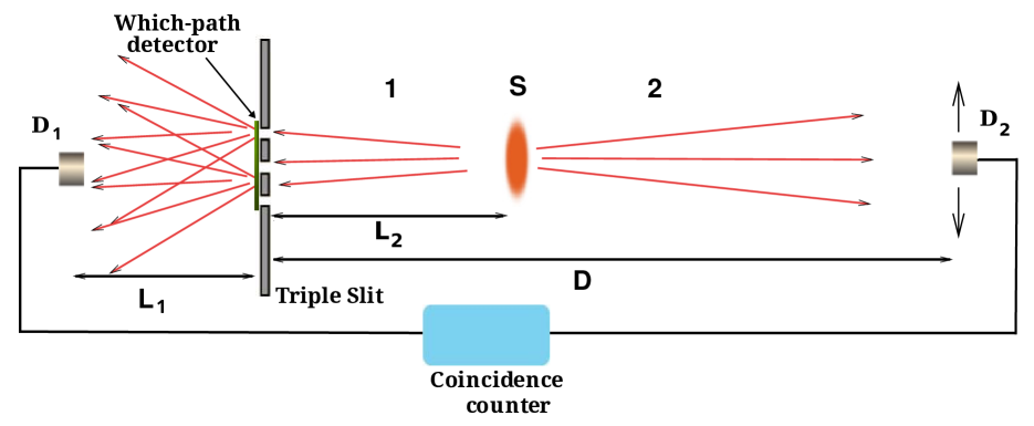
Figure 3: Three-slit ghost interference experiment, when which-way detector is placed behind the slits.

To find the duality relation, we place the which-way detector behind the three slits, (see FIG. 3), by which the experimenter gets which-path information. The which-way detector chosen with three states, correlate with the particle, when it passes through each slit. Let the path-detector states be $|d_{1}\rangle,|d_{2}\rangle,|d_{3}\rangle$, which correspond to the particle passing through slit 1, 2 and 3, respectively. Without the loss of generality, we assume that the states $|d_{1}\rangle,|d_{2}\rangle,|d_{3}\rangle$ are normalized, but not necessarily mutually orthogonal.

A fundamental property of quantum mechanics is that a state cannot be perfectly distinguished by any physical device, unless they are orthogonal. However, if a non-zero probability of inconclusive answer is allowed, one can certainly distinguish the given sates. This idea was introduced by Ivanoviciva , Dieksdiek and Perespere and is called unambiguous quantum state discrimination(UQSD). The above strategy can be used to gain the information about the path taken by the particle in interference experiments.

If path-detector states $|d_{1}\rangle,|d_{2}\rangle,|d_{3}\rangle$ are mutually orthogonal, one can get the information about the path of the particle, without ambiguity. For non-orthogonal states $|d_{1}\rangle,|d_{2}\rangle,|d_{3}\rangle$ we use an UQSD technique to define distinguishabilityasad , for three slit interference.

$${\mathcal{D}_{Q}}\equiv 1-{1\over 3}(|\langle d_{1}|d_{2}\rangle|+|\langle d_{2}|d_{3}\rangle|+|\langle d_{1}|d_{3}\rangle|),$$ (21)

The which-way distinguishability for particle 1 is given by

$${\mathcal{D}^{1}_{Q}}\equiv 1-{1\over 3}(|\langle d_{1}|d_{2}\rangle|+|\langle d_{2}|d_{3}\rangle|+|\langle d_{1}|d_{3}\rangle|),$$ (22)

the value lies in the range $0\leq{\mathcal{D}^{1}_{Q}}\leq 1$.

Let us see the effect of which-path detector on the ghost interference given by particle 2. We assume that the two particles move in opposite directions along the x-axis, and the entanglement is in the z-direction.

The particle 1 is then made to interact with which-path detector, which gives rise to an entanglement between the two particles and the which-path detector.

We get the following states.

$$\Psi(z_{1},z_{2},t) = C_{t}\Bigg{(}|d_{1}\rangle\exp\left[{{-(z_{1}-z_{0})^{2}\over\epsilon^{2}+{iL_{1}\lambda\over\pi}}}\right]\exp\left[{{-(z_{2}-z_{0}^{\prime})^{2}\over\Gamma+{iL_{1}\lambda\over\pi}}}\right]$$

$$+ |d_{2}\rangle\exp\left[{{-z_{1}^{2}\over\epsilon^{2}+{iL_{1}\lambda\over\pi}}}\right]\exp\left[{{-z_{2}^{2}\over\Gamma+{iL_{1}\lambda\over\pi}}}\right]$$

$$+ |d_{3}\rangle\exp\left[{{-(z_{1}+z_{0})^{2}\over\epsilon^{2}+{iL_{1}\lambda\over\pi}}}\right]\exp\left[{{-(z_{2}+z_{0}^{\prime})^{2}\over\Gamma+{iL_{1}\lambda\over\pi}}}\right]\Bigg{)},$$

where

$$C_{t}={\sqrt{2}\over\sqrt{3\pi}\sqrt{\epsilon+iL_{1}\lambda/\epsilon\pi}\sqrt{\sqrt{\Gamma_{r}}+(\Gamma_{i}+iL_{1}\lambda/\pi)/\sqrt{\Gamma_{r}}}}.$$

The probability density at $z_{1}=0$, given by $|\Psi(0,z_{2},t)|^{2}$, has the following form

$$|\Psi(0,z_{2},t)|^{2} = |C_{t}|^{2}\Bigg{[}\exp\left[\frac{-2z_{2}^{2}}{\gamma_{D}^{2}}\right]\Bigg{(}1+2\cosh\left[\frac{4z_{2}z_{0}}{\gamma_{D}^{2}}\right]$$

$$\times \exp\left[\frac{-2z_{0}^{2}}{\epsilon^{2}+(\frac{\lambda L_{1}}{\pi\epsilon})^{2}}-\frac{2z_{0}^{2}}{\gamma_{D}^{2}}\right]\Bigg{)}+2~{}|\langle d_{1}|d_{2}\rangle|$$

$$\times \exp\left(\frac{-z_{0}^{2}}{\epsilon^{2}+(\frac{\lambda L_{1}}{\pi\epsilon})^{2}}-\frac{2z_{2}^{2}+z_{0}^{2}-2z_{2}z_{0}}{\gamma_{D}^{2}}\right)$$

$$\times \cos\left[2z_{2}z_{0}\xi_{2}-z_{0}^{2}(\xi_{1}+\xi_{2})\right]$$

$$+ 2~{}|\langle d_{1}|d_{3}\rangle|\exp\left(\frac{-2z_{0}^{2}}{\epsilon^{2}+(\frac{\lambda L_{1}}{\pi\epsilon})^{2}}-\frac{2(z_{2}^{2}+z_{0}^{2})}{\gamma_{D}^{2}}\right)$$

$$\times \cos\left[4z_{2}z_{0}\xi_{2}\right]$$

$$+ 2~{}|\langle d_{2}|d_{3}\rangle|\exp\left(\frac{-z_{0}^{2}}{\epsilon^{2}+(\frac{\lambda L_{1}}{\pi\epsilon})^{2}}-\frac{2z_{2}^{2}+z_{0}^{2}+2z_{2}z_{0}}{\gamma_{D}^{2}}\right)$$

$$\times \cos\left[2z_{2}z_{0}\xi_{2}+z_{0}^{2}(\xi_{1}+\xi_{2})\right]\Bigg{]},$$

where

$$\xi_{1}={\lambda L_{1}/\pi\over\epsilon^{4}+(\lambda L_{1}/\pi)^{2}},~{}~{}~{}\xi_{2}={\lambda D/\pi\over\gamma^{4}+(\lambda D/\pi)^{2}},$$

Visibility of the interference fringes is conventionally defined asborn

$${\mathcal{V}}={I_{max}-I_{min}\over I_{max}+I_{min}},$$ (25)

where $I_{max}$ and $I_{min}$ represent the maximum and minimum intensity in neighbouring fringes, respectively. Maxima and minima of (LABEL:peter) will occur at points where the value of each cosine is 1 and -1/2 , respectively, provided we ignore $z_{0}^{2}(\xi_{1}+\xi_{2})$ term. If we look at any fringe, other than the central one, $z_{0}\ll z_{2}$, and hence can be ignored in comparison.

The visibility of particle 2 can then be written down as

$${\mathcal{V}}_{2}={3\left(|\langle d_{1}|d_{2}\rangle|e^{{2z_{2}z_{0}\over\gamma_{D}^{2}}}+|\langle d_{1}|d_{3}\rangle|e^{-z_{0}^{2}\zeta}+|\langle d_{2}|d_{3}\rangle|e^{{-2z_{2}z_{0}\over\gamma_{D}^{2}}}\right)\over\alpha+|\langle d_{1}|d_{2}\rangle|e^{{2z_{2}z_{0}\over\gamma_{D}^{2}}}+|\langle d_{1}|d_{3}\rangle|e^{-z_{0}^{2}\zeta}+|\langle d_{2}|d_{3}\rangle|e^{{-2z_{2}z_{0}\over\gamma_{D}^{2}}}}.$$ (26)

where,     $\zeta=\left[\frac{1}{\epsilon^{2}+(\frac{\lambda L_{1}}{\pi\epsilon})^{2}}+\frac{1}{\gamma_{D}^{2}}\right],$    and

$\alpha=2\left(\exp[\frac{z_{0}^{2}}{\gamma_{D}^{2}}]+2\exp[-{z_{0}^{2}\zeta}]\cosh[\frac{4z_{2}z_{0}}{\gamma_{D}^{2}}]\right)$,

The maximum visibility one can theoretically get when $z_{0}\ll\frac{\lambda L_{1}}{\pi}$, and $z_{0}\ll\frac{\lambda D}{\pi}$. The actual fringe visibility will be less than or equal to that, and can be written as

$${\mathcal{V}_{2}}\leq{3\left(|\langle d_{1}|d_{2}\rangle|+|\langle d_{1}|d_{3}\rangle|+|\langle d_{2}|d_{3}\rangle|\right)\over 2\left(1+2\right)+|\langle d_{1}|d_{2}\rangle|+|\langle d_{1}|d_{3}\rangle|+|\langle d_{2}|d_{3}\rangle|}.$$ (27)

Using (22), the above equation gives

$${\mathcal{V}_{2}}+{2{\mathcal{D}^{1}_{Q}}\over 3-{\mathcal{D}^{1}_{Q}}}\leq 1.$$ (28)

The duality relation (28), is very similar to the duality relation derived earlier for a three-slit interference experimentasad . The big difference is that, in three-slit experiment we talk of the path distinguishability and the fringe visibilty for the same particle. In three-slit ghost interference, we show that the relation is between different particles, i.e the path distinguishability of particle 1 is related with the fringe visibilty of particle 2.

If instead of triple slit, a double slit were kept in the path, the path distinguishability of particle 1 and the fringe visibilty of particle 2, will follow a different duality relation, given by ${\mathcal{V}_{2}}+{\mathcal{D}^{1}_{Q}}\leq 1$. This can be inferred by relating $D_{Q}$ with distinguishability used in Ref. [tabish ].

V Conclusion

In conclusion, we have analyzed the complementarity between which-way information and interference fringe visibility for the ghost interference, for entangled photons passing through three slits. We also derive a three-slit nonlocal duality relation which connects the path distinguishability of one photon to the interference visibility of the other which means erasing the which-path information of photon 1 recovers the interference pattern of photon 2 and vice-versa.

References

• (1) M. A. Nielsen and I. L. Chuang, Quantum Computation and Quantum Information (Cambridge University Press, Cambridge, UK, 2000).
• (2) R. Horodecki, P. Horodecki, M. Horodecki and K. Horodecki, Rev. Mod. Phys. 81 (2009) 865.
• (3) T. B. Pittman, Y. H. Shih, D. V. Strekalov, and A. V. Sergienko, Phys. Rev. A 52 (1995) R3429.
• (4) A. K. Ekert,Phys. Rev. Lett. 67 (1991) 661.
• (5) D.V. Strekalov, A.V. Sergienko, D.N. Klyshko, Y.H. Shih, Phys. Rev. Lett. 74 (1995) 3600.
• (6) D. N. Klyshko, Photon and Nonlinear Optics, Gordon and Breach Science, New York, (1988); Β A. Yariv, Quantum Electronics, John Wiley and Sons, New York, (1989). β€œSpontaneous Parametric Down Conversion” was called β€œSpontaneous Fluorescence” and β€œSpontaneous Scattering” by the pioneer workers.
• (7) P. G. Kwiat, K. Mattle, H. Weinfurter, A. Zeilinger, A. V. Sergienko, and Y. H. Shih, Phys. Rev. Lett. 75 (1995) 4337.
• (8) S. P. Walborn and C. H. Monken, Phys. Rev. A 76 (2007) 062305.
• (9) M. D’Angelo, Y-H. Kim, S. P. Kulik and Y. Shih, Phys. Rev. Lett. 92 (2004) 233601 .
• (10) S. P. Walborn, C.H. Monken, S. PΓ‘dua, P.H. Souto Ribeiro, Phys. Rep. 495 (2010) 87.
• (11) N. Bohr, Nature (London) 121 (1928) 580.
• (12) D. M. Greenberger and A. Yasin, Phys. Lett. A 128 (1988) 391.
• (13) B.-G. Englert, Phys. Rev. Lett. 77 (1996) 2154 .
• (14) M. A. Siddiqui, T.Qureshi, arXiv:1406.1682 [quant-ph].
• (15) S. DΓΌrr, Phys. Rev. A 64 (2001) 042113 .
• (16) A. Luis, Phys. Rev. A 67 (2003) 032108.
• (17) G. Bimonte and R. Musto, Phys. Rev. A 67 (2003) 066101; J. Phys. A 36 (2003) 11481.
• (18) M. Jakob and J. A. Bergou, Int. J. Mod. Phys. B 20 (2006) 1371 ; Phys. Rev. A 76 (2007) 052107.
• (19) B.-G. Englert, D. Kaszlikowski, L.C. Kwek, and W. H. Chee, Int. J. Quant. Info. 06 (2008) 129.
• (20) M. A. Siddiqui, T. Qureshi, arXiv:1405.5721 [quant-ph].
• (21) G. Weihs, M. Reck, H. Weinfurter and A. Zeilinger, Opt. Lett. 21 (1996) 302.
• (22) M. Zawisky, M. Baron, and R. Loidl, Phys. Rev. A 66 (2002) 063608.
• (23) U. Sinha, C. Couteau, T. Jennewein, R. Laflamme, G. Weihs, Science 329 (2010) 418.
• (24) S. Frabboni, C. Frigeri, G.C. Gazzadi, and G. Pozzi, American Journal of Physics 79 (2011) 615.
• (25) C. Ududec, H. Barnum and J. Emerson, Foundations of Physics 41 (2011) 396.
• (26) H. DeRaedt, K. Michielsen, K. Hess, Phys. Rev. A 85 (2012) 012101 .
• (27) G. Niestegge, Foundations of Physics 43 (2013) 805; Phys. Scr. T160 (2014) 014034.
• (28) R. Sawant, J. Samuel, A. Sinha, S. Sinha, U. Sinha, Phys. Rev. Lett. 113 (2014) 120406.
• (29) E. Gagnon, C. D. Brown, and A. L. Lytle, Phys. Rev. A 90 (2014) 013832.
• (30) A. J. GutiΓ©rrez-Esparza, W. M. Pimenta, B. Marques, A. A. Matoso, J. L. Lucio M., and S. PΓ‘dua, Opt. Express 20 (2012) 26351.
• (31) A. J. GutiΓ©rrez-Esparza, W. M. Pimenta, B. Marques, A. A. Matoso, J. Sperling, W. Vogel, and S. PΓ‘dua, Phys. Rev. A 90 (2014) 032328.
• (32) P. Kolenderski, U. Sinha, L. Youning, T. Zhao, M. Volpini, A. Cabello, R. Laflamme, and T. Jennewein, Phys. Rev. A 86 (2012) 012321.
• (33) G. Taguchi, T. Dougakiuchi, M. Iinuma, H. F. Hofmann, and Y. Kadoya, Phys. Rev. A 80 (2009) 062102.
• (34) W. M. Pimenta, B. Marques, T. O. Maciel, R. O. Vianna, A. Delgado, C. Saavedra, and S. PΓ‘dua, Phys. Rev. A 88 (2013) 012112.
• (35) D. N. Klyshko, Uspekhi Fizicheskikh Nauk 154 (1988) 133.
• (36) T. Qureshi, P. Chingangbam, S. Shafaq, arXiv:1406.0633 [quant-ph].
• (37) T. Qureshi, Am. J. Phys. 73 (2005) 541.
• (38) A. Einstein, B. Podolsky, N. Rosen, Phys. Rev. Lett. 47 (1935) 777.
• (39) I. D. Ivanovic, Phys. Lett. A 123 (1987) 257.
• (40) D. Dieks, Phys. Lett. A 126 (1988) 303.
• (41) A. Peres, Phys. Lett. A 128 (1988) 19.
• (42) M. Born, E. Wolf, Principles of Optics, 7th edn. (Cambridge University Press, UK, 2002).