2D2C, 2D3C, 2C2Dcw1C3D, 3D3C, rotating turbulence, thin-layer flows, quasi-static magnetohydrodynamics (QSMHD), and beyond

Abstract

More serious works on 2D2C, 2D3C, 2C2Dcw1C3D, 3D3C, rotating turbulence, thin-layer flows, quasi-static magnetohydrodynamics (QSMHD), and all that are wanted, but we report timely here some studies on locally and globally 2C2Dcw1C3D flows, with the hope to promote smarter and deeper works.

0 Preamble

See pages 1- of rsfinclude.pdf

1 Introduction

The governing equations for our two-dimensional (2D) passive scalar turbulence problem are

$$\partial_{t}\theta+\bm{v}\cdot\nabla\theta = \kappa\nabla^{2}\theta+f_{\theta},$$ (1)

$$\partial_{t}\bm{v}+\bm{v}\cdot\nabla\bm{v} = -\nabla P+\nu\nabla^{2}\bm{v}+f_{\bm{v}},\ \nabla\cdot\bm{v}=0,$$ (2)

where $f_{\bullet}$ denotes forcing. The scalar $\theta$ is passive because of no back-reaction onto $\bm{v}$ with $f_{\bm{v}}$ independent on $\theta$ (otherwise active), and $\bm{v}$ is the classical incompressible 2D Navier-Stokes velocity field with $f_{\bm{v}}$ independent of $\bm{v}$, in particular with $f_{\bm{v}}=0$ and that the pressure $P$ being related to $\bm{v}$ by the Poisson equation $-\partial_{\alpha\alpha}P=\partial_{\beta\gamma}(v_{\beta}v_{\gamma})$. Curling (2), we have

$$\partial_{t}\zeta+\bm{v}\cdot\nabla\zeta=\nu\nabla^{2}\zeta+f_{\zeta},$$ (3)

with the vertical vorticity $\zeta\bm{z}=\bm{\zeta}=\nabla\times\bm{v}$, which is intrinsically different to the passive scalar in Eq. (1). The full 3D incompressible Navier-Stokes equations with $\partial_{z}=0$, i.e., depending only on $x$ and $y$ coordinates, or alternatively, averaged over $z$, becomes such a 2D-three-component (2D3C) system and the vertical velocity $\bm{u}_{z}=u_{z}\bm{z}=\theta\bm{z}$ in the (unit) $\bm{z}$ direction is passively advected by the horizontal velocity $\bm{u}_{h}$ in the $x-y$ plane, thus a problem of 2D passive scalar with unit Prandtl number $\nu/\kappa$. [Note that we have used $\bm{u}$ to represent the general velocity field, instead of $\bm{v}$ for that in the $x-y$ plane; that is, $\bm{u}_{h}=\bm{v}$.] The problem we focused on is the possibility of different spectral transfer dynamics of the passive scalar energy like various active scalars, with multidisciplinary physical relevance. Starting from this section, we will subsequently present collectively four favorable arguments. There are new ideas and/or techniques in each argument, which requires careful reasoning and thus somehow (re)formulating the relevant background materials with reasonable details. Experienced readers can jump to the end of this section for a summary of our arguments and then, without strictly following our formulation of the problems, selectively look for our reasoning in each section.

2D3C (dominant) dynamics also emerge in the quasi-static magnetohydrodynamics (QSMHD — cf., e.g., Favier et al. [1] and references therein) due to extra linear Ohmic anisotropic dissipation operator, effectively different damping rate $\propto cos^{2}\theta=k_{z}^{2}/k^{2}$ on different cone surfaces of $\bm{k}$s forming different angles $\theta$s with the background magnetic field direction $\bm{z}$ (“‘conical’ Joule dissipation effect” responsible for the ‘directional’ anisotropy [2] and thus two-dimensionalization [3, 2]). Yet another situation, in which 2D3C dynamics can arise and that also can be reformulated to be due to anisotropic dissipation, is the so-called thin-layer flows, and there have been documentations on the transitions from 2D to 3D or from inverse- to co-existing/split and to forward cascades in the simulations with periodic boundary conditions, not ‘bounded’ or ‘without boundaries’ (see, e.g., Smith et al. [4] and Celani et al. [5]). Since, to our best knowledge, there is not any formulation for the two-dimensionalization of this latter intuitive case, let us show here that simple scale-normalization argument makes the scenario quite transparent: Suppose the box dimensions in $x$, $y$ and $z$ directions are $L_{z}R=L_{x}=L_{y}=L$, then by scale transformation $z^{\prime}=zR$ it is direct to see, with corresponding re-scaling of the vertical velocity and forcing (pressure can be canceled by incompressibility), that we have effectively new anisotropic viscosity $\nu_{z^{\prime}}R^{-2}=\nu_{x}=\nu_{y}=\nu$: The anisotropic viscosities lead to anisotropic viscous scales, and the dynamics should be understood with corresponding re-scaling of the forcing scales (if exist). The much larger $\nu_{z^{\prime}}$ with large $R$ smoothes $z^{\prime}$ dynamics more, leading to much smaller $\partial_{z^{\prime}}$ (formally $\to 0$ with $R\to\infty$), i.e., asymptotically 2D3C. Especially, if the vertical forcing scale in $z^{\prime}$ is smaller than the vertical dissipation scale $\eta_{z^{\prime}}$, then $z^{\prime}$-direction motions can hardly take effect. There are also other mechanisms of two-dimensionalization, such as strong background magnetic field in a plasma or strong rotation of a neutral fluid: Perturbative arguments for the magnetohydrodynamics case for the former was given by Montgomery and Turner [6], say; the latter will be used and elaborated a bit more later. Note that quasi-two-dimensionalization in all these cases are quite obviously documented in experiments and numerical simulations and are easy to understand physically, though whether the pure 2D dynamics can be rigorously obtained in the corresponding limits may sometimes be subtle and even controvertible.

For the 2D3C dynamics, how the passive scalar is affected by the advecting dynamics is measured by their cross-correlations. It turns out that the one as the integral over the volume $\mathcal{V}$ of the $\bm{r}$ ($=[x,y]$) space of the passive scalar and the vertical vorticity,

$$\mathcal{C}=2\langle\zeta\theta\rangle=\frac{2}{\mathcal{V}}\int\zeta\theta d\bm{r},$$ (4)

is an ideal dynamical quadratic invariant (at least formally). [With the ergodicity assumption, the volume average equals the statistical average, thus sharing the same notation $\langle\cdot\rangle$. The factor of $2$ is simply for later convenience.] Due to the fact that both $\theta$ and $\zeta$ are Lagrangian invariants, the multiplication of respectively any function of their own is also formally a Lagrangian invariant. In this sense, this 2D3C situation appears to be quite unique among all the $d$-dimensional problems. This $\mathcal{C}$ is quadratic and ‘rugged’ (see below). It actually is the reduced helicity [7]; see also Sec. 3 where the relation and difference to the ‘vertical/horizontal helicity (density)’ frequently referred to in weather science are noted. Helicity is an ideal rugged invariant, i.e., conserved with or without spectral truncation [8]. So, it is intriguing whether $\mathcal{C}$ is controllable and what its dynamical effects are.

Note that the probability notion of ‘statistical correlation’ does not distinguish the asymmetrical dynamical dependence, which may bring subtleties into the problem of passive scalar with explicit dynamically asymmetrical dependence: the scalar depends on the advecting field, but not the reverse. Simple statistical/probabilistic description by itself is inadequate/incomplete for dynamical systems: Here, due to dynamical dependence of $\theta$ on $\zeta$, it is possible to have covariance between them. The covariance statistically, but not dynamically, also means linear dependence of $\zeta$ on $\theta$; also, from the joint Gaussian distribution of the applied Gibbs ensemble for the absolute equilibrium (see later discussions), zero covariance would indicate statistical independence between them. Further more, a way to control $\mathcal{C}$ is to have $f_{\theta}$ be appropriately correlated to the advecting dynamics, say, a reasonable $\langle f_{\theta}\zeta\rangle$ which by itself however could result from dynamical dependence of $\zeta$ on $f_{\theta}$, which is not the case for passive scalar problem. [Statistical description in principle can be infinitely complex, with, for instance, infinitely-many-dimensional (conditional) probability distribution functions (PDFs) or moments, so by ‘simple’ the limitations of finiteness of the PDFs or moments are referred to.] So, $\mathcal{C}$ itself and its control present some ambiguity with the passive and active scalars; or, in other words, controlling $\mathcal{C}$ for the passive scalar bridges the problem to the active scalar one. However, according to the dynamics, as long as there is no back-reaction onto the advecting field, the problem is still of passive nature.

Ref. [9]’s review, of active versus passive scalars due to the progresses [10] of the Kraichnan model [11], revisits the inverse cascade of the active magnetic potential energy (the root mean square of the ‘flux function’, the vertical component of the vectorial potential) of two-dimensional (2D) magnetohydrodynamics (MHD) [12]. The relevant result may actually be used to make the conjecture of the possibility of similar statistics for some special passive scalars, beyond the very limited Kraichnan model and with some similar necessary mechanisms of 2D MHD, which constitutes the important point of this study. Our study will also be assisted with the analysis of turbulence in a rotating frame of coordinates. We know that in the small-Rossby-number limit, in particular situations and regimes, the system contains a self-autonomous 2D3C subdynamics with the vertically-averaged vertical velocity being a passive scalar. In general, the pure 2D limit may not be unconditionally reached: The relevant time scales for different non-resonant modes are continuously non-uniform, depending on how ‘near’ to the resonant condition they are [14], which, together with the nonlinearity of near-resonant interactions (unlike the linear an-isotropic damping in QSMHD), makes the decoupling issue extremely subtle. For example, Chen et al. [15] showed that the long-time errors between the vertically-averaged results and the pure 2D one grow, ‘implying non-resonant effects’ and ‘is consistent with’ closure theories [16]. And, Smith and Lee [17] found, by examining the near-resonant, near-2D, pure-2D and full-3D interactions, that near-resonant but not near-2D interactions were responsible for the special 2D large-scale properties of 3D rotating flows, that distinguished from the pure 2D ones, such as the steeper energy spectra and the dominance of cyclones over anticyclones. They also noted that the pure 2D interactions are necessary for the generation of 2D large-scales. Of course, there may be subtle differences between the geometries of a finite cyclic box and an infinite domain, and there may be issues of discreteness and resolution effects, as noted by a series of interesting works of Cambon and collaborators [18, 19, 16] and as addressed, e.g., by Bourouiba and co-workers [20, 21]. Recently there are numerical simulations with intermediate/moderate Rossby numbers by two independent working groups [15, 22], showing indeed large-scale formation of the vertically-averaged vertical velocity, while Chen et al. [15] noticed that simulations with even smaller Rossby number do not show the corresponding inverse transfers. Bourouiba and Bartello [20] also particularly identified and examined the ‘intermediate-Rossby-number’ regime which presents special properties and to which previous relevant simulations by Smith and collaborators and Chen et al. [23, 15, 17] were claimed to belong. To try to understand the role of the 2D3C subdynamics embedded in the full 3D3C system, in Sec. 4 we thus focus on this issue and speculate the triggering of spontaneous chirality (mirror symmetry breaking) only with sufficient wave-vortex coupling in this regime. A further speculation of 2D3C dominated helical cyclogenesis will be proposed in Sec. 6. A modification of the Kraichnan model with preliminary calculations will also be presented in Sec. 5 to bring further insights for possible systematic solution of the problem. The absolute equilibrium analysis of this work was originally a ‘byproduct’ of Ref. [24] and was meant to be added to it at its late stage, particularly addressing the numerical reports of Refs. [25, 26], so a relevant briefing, but with extra perspectives, is given in the Appendix.

In summary, our main objective is to clarify the conjecture of the possible non-universal genuine transfer directions of two-dimensional (2D) passive scalar energy, given the inversely cascaded (to large scales) advecting velocity, and collectively four arguments are used. In the following sections, we will present 1), the reasoning with the comparison between passive and inversely-cascaded active scalars, given in this introductory discussion, and we will offer 2), the absolute-equilibrium spectra shown concentration of 2D passive scalar energy at both large- and small-scale ends, 3), the detailed analysis and explanation of the inverse transfers of the vertically averaged vertical velocity in moderate-Ro rotating flows, together with 4), preliminary calculation of a modified Kraichnan model showing how the details of the passive scalar pumping mechanism matters. Remarks on helicity in other situations and ‘vertical helicity’ in hazardous weather also follow.

2 Reflection on active and passive fields: a new perspective

Ref. [9] reviews the studies on ‘active and passive fields face to face’, following the developments due to the progresses of the Kraichnan model [11] (see Ref. [10] and references therein). Not surprisingly, active scalars such as 2D temperature/density, magnetic potential and vorticity etc. are different - nonuniversal, both in the sense of the transfer directions and the inertial-range scaling laws. As a sidenote, we remark that the conventional notion of universality in the Kraichnan model refers to the independence of the scaling exponents on the ‘details of the pumping’ of the passive scalar [10]. The pumping of the Kraichnan model is an independent Gaussian white-in-time field with prescribed spacial correlation on which the scaling exponents are independent. Beyond the Kraichnan model, the details of the pumping are rich, including possible correlations with other variables, and may affect the passive scalar statistics - the scaling exponents and others. The interesting behaviors of active scalars, such as the inverse cascade of the magnetic potential energy of 2D MHD, is related to the statistical correlation of the pumping with the particle/tracer trajectories, i.e., the advecting field. Such a correlation can be traced to the back-reaction through $f_{\bm{v}}$ and in general is absent for the passive scalar, even that advected by the same realization of velocity and pumped by ‘statistically the same’ (in the sense of its own probability distribution function) but different independent realization of $f_{\theta}$ [9]. However, we note that even for the passive scalar problem, given the same velocity field, there in principle can exist realizations of the pumping, controlled artificially or by nature, to have various statistical correlations with the particle trajectories, resulting in, presumably, different statistics, including all the possible ones of active and passive scalars in literatures. Of course the passive scalar inverse transfer, as the one of the active magnetic potential energy (the root mean square of the ‘flux function’, the vertical component of the vectorial potential) of two-dimensional (2D) magnetohydrodynamics (MHD), first predicted from the absolute equilibrium argument [12], is in the list. As noted in the end of the last paragraph, this may require some adjustments of the traditional understanding of passive scalar problem but is not really complete new: for instance, Holzer and Siggia [13] took the pumping be the velocity projected onto a constant vector (taken to be the background gradient of the scalar in Ref. [13]). Thus the above analysis already leads us to the conjecture of nonuniversal transfer directions of passive scalars, especially the possibility of inverse cascade/transfer of 2D passive scalar which will be further augmented with absolute-equilibrium analysis by novel inclusion of the dynamical effects of $\mathcal{C}$ (Sec. 3). As another sidenote, since we come to the issue of inverse cascade/transfer of the passive scalar, we remark that its existence or not is not necessarily related to the existence or absence of the so-called dissipative anomaly, i.e., the persistent dissipation in the vanishing diffusivity: With dissipative anomaly, it only means that some energy is dissipated at small scales, which does not necessarily excludes inverse cascade/transfer at large scales. [And, without dissipative anomaly, energy could resides in some regime, which does not necessarily imply inverse cascade/transfer.]

3 $\mathcal{C}$-containing absolute equilibrium

For a 2D3C passive scalar advection the rugged invariants are the (horizontal) kinetic energy $\mathcal{E}=\langle u_{h}^{2}\rangle,$ the enstrophy $\mathcal{W}=\langle\zeta^{2}\rangle,$ and the passive-scalar (vertical) energy $\mathcal{Z}=\langle\theta^{2}\rangle=\langle u_{z}^{2}\rangle,$ besides $\mathcal{C}$, Eq. (4). We now show that the cross-correlation $\mathcal{C}$ is equivalent to the well-known invariant helicity [7] under appropriate conditions: With $\bm{\zeta}=\nabla\times\bm{u}_{h}$ and $\theta=u_{z}$, we have $\int\int\zeta\theta dxdy=\int\int\nabla\times\bm{u}_{h}\cdot\bm{u}_{z}dxdy.$ One can easily check by integration by parts, assuming vanishing velocity at the boundary, say, infinity, or by assuming periodic boundary condition, that

$$\int\int\nabla\times\bm{u}_{h}\cdot\bm{u}_{z}dxdy=-\int\int\bm{z}\times\nabla u_{z}\cdot\bm{u}_{h}dxdy.$$

Thus now $\mathcal{C}=2\langle\zeta\theta\rangle$ is nothing but the reduced form of the well-known helicity, since, when $\partial_{z}\bm{u}=0$, the integrand of helicity

$$\nabla\times\bm{u}\cdot\bm{u}=\nabla\times\bm{u}_{h}\cdot\bm{u}_{z}-\bm{z}\times\nabla u_{z}\cdot\bm{u}_{h}.$$

[And, then issues such as the (detailed) conservation laws of $\mathcal{C}$ etc. are reduced to what we know how to solve from [8].] Note that the local density of $\mathcal{C}$ is not $2\theta\zeta$ but

$$\theta\zeta-\bm{z}\times\nabla\theta\cdot\bm{u}_{h}.$$

For $\bm{u}$ in a cyclic box with dimension $2\pi$, we have the Fourier representation $\bm{u}(\bm{r})=\sum_{\bm{k}}\hat{\bm{u}}_{\bm{k}}\exp\{\hat{i}\bm{k}\cdot\bm{r}\}$ and further expansion with the self-evident notations $\bm{k}_{h}$ and $\bm{k}_{z}$ (following those of the physical-space variables — all complex variables are consistently wearing hats in this paper and $\hat{i}$ is the pure imaginary unit): For the incompressible 2D flow, denoting the horizontal wavevector by $\bm{k}_{h}$, we have $\hat{\bm{u}}_{h}\cdot\bm{k}_{h}=0$ and are left with only one degree of freedom in the direction $\bm{h}(\bm{k}_{h})=\bm{z}\times\bm{k}_{h}/k_{h}$ for $\hat{\bm{u}}_{h}$; so, writing $\hat{\bm{u}}_{h}=\hat{u}_{h}(\bm{k}_{h})\bm{h}(\bm{k}_{h})$, we have

$$\mathcal{C}=\tilde{\sum}\hat{i}k_{h}(\hat{u}_{h}\hat{u}_{z}^{*}-c.c.),\ \mathcal{E}=\tilde{\sum}|\hat{u}_{h}|^{2},\ \mathcal{W}=\tilde{\sum}k_{h}^{2}|\hat{u}_{h}|^{2}\ \textnormal{and}\ \mathcal{Z}=\tilde{\sum}|\hat{u}_{z}|^{2},$$

where we have applied the conventional Galerkin truncation keeping only modes with $k_{min}\leq|\bm{k}_{h}|\leq k_{max};\ \textnormal{thus}\ \tilde{\sum}\triangleq\sum_{k_{min}\leq|\bm{k}_{h}|\leq k_{max}}.$ ‘$\triangleq$’ means definition, and for simplicity, we have omitted the conventional factors of $1/2$ which can be absorbed into the (inverse) temperature parameters (see below). [Alternatively, following the notion of helical inertial waves of rotating flows [27], the helical representation (see below) in 2D reduces to $\hat{v}_{+}=-\hat{v}_{-}$; so, one may use $\hat{\bm{u}}_{h}=\hat{u}^{\prime}_{h}(\bm{k}_{h})\hat{\bm{h}}^{\prime}(\bm{k}_{h})$ with $\hat{\bm{h}}^{\prime}(\bm{k}_{h})=\hat{i}\bm{z}\times\bm{k}_{h}/k_{h}$, and yet another way for interested readers to exercise and check the calculations is starting with the Fourier expansion of the familiar stream function $\bm{\psi}=\psi\bm{z}$ for the horizontal flow, with $\bm{v}=-\nabla\times\bm{\psi}$ and $\bm{\zeta}=\nabla^{2}\bm{\psi}$.] It is direct to check that all these quadratic invariants are conserved in detail for each interacting triad and that, together with their global conservation laws, the quadratic and diagonal properties ensure their ruggedness after arbitrary truncations [8], which justifies respecting all of them in the statistical treatment.

For the Galerkin-truncated inviscid and diffusionless system, triadic interactions of the modes through the convolution in the convective terms in general will present chaotic dynamics and lead to thermalization, i.e., approaching the thermal equilibrium. Indeed, as shown by Lee [28] for 3D incompressible hydrodynamics, the ordinary dynamical system in terms of the Fourier modes satisfies the Liouville theorem which ensures an invariant measure. Similar result was also obtained by Hopf [29] who applied functional calculus to formally derive it, but without explicitly introducing the Galerkin truncation. [The classical wisdom is that the physical measure may be accurately represented by the Gibbs state, at least for low order moments.] And, such fundamental dynamics should play a central role for many properties of the dissipative (and diffusive) turbulence; the spectral transfer property should be signatured by such an internal drive of thermalization. Recently Moffatt [30] studied the single-triad interactions, but for statistical considerations we in general need “many” [31] triads (still, the thermalization assumption fails for however many triads if the superposed Fourier modes result in vanishing nonlinearity [33]); otherwise, other unknown invariants might emerge or ergodicity might seriously break down [31, 32]. Besides other possible footprints, the statistical absolute equilibria set up the aims towards which the distribution of the spectra tend to relax [34, 8], thus some clues of cascade directions may be obtained. However, before proceeding, we should point out that, although successful in many aspects, such an approach nevertheless misses many other ingredients of the dynamics, which makes it in general difficult to conclude from the results very accurately and firmly about turbulence; and, a caveat particular to the passive scalar problem is that the calculations can not exploit the passiveness of the scalar, as is a particular case of the inadequacy/incompleteness of simple statistical description remarked in the introductory discussion. Some finer statistical treatment than the conventional microcanonical ensemble may be necessary to be more precise. We should view the absolute equilibrium calculation as a unique mathematical treatment to expose fundamental aspects of the dynamics. Recently, the idea has been extended to study explicitly realizable fractally decimated [35] and also some chirally selected ([36] and references therein) Navier-Stokes systems, and, besides transfer directions, insights about the isotropic polarization issue and similarly multiple-constraint nonequilibrium dynamical ensembles [37, 38] can be motivated [39].

Introducing corresponding Lagrange multipliers or the (inverse) temperature parameters $\Gamma_{\bullet}$, we now apply the Gibbs distribution, i.e., the canonical ensemble with constant temperature parameters assigning a probability $\mathcal{P}$ to each microstate

$$\mathcal{P}\sim\exp\{-(\Gamma_{\mathcal{C}}\mathcal{C}+\Gamma_{\mathcal{E}}\mathcal{E}+\Gamma_{\mathcal{W}}\mathcal{W}+\Gamma_{\mathcal{Z}}\mathcal{Z})\},$$

to obtain the modal spectral densities, $U_{h}$ of $\mathcal{E}$, $W$ of $\mathcal{W}$, $Q_{\mathcal{C}}$ of $\mathcal{C}$ and $U_{z}$ of $\mathcal{Z}$:

$$\!\!\!\!\!\!\!\!\!\!\!\!\!\!\!\!\text{with}\ \ D=\Gamma_{\mathcal{E}}\Gamma_{\mathcal{Z}}+(\Gamma_{\mathcal{W}}\Gamma_{\mathcal{Z}}-\Gamma_{\mathcal{C}}^{2})k_{h}^{2}>0,\ U_{h}\triangleq\langle|\hat{u}_{h}|^{2}\rangle=\frac{\Gamma_{\mathcal{Z}}}{D{\color[rgb]{1,0,0}}},\ W=k_{h}^{2}U_{h},$$ (5)

$$\!\!\!\!\!\!\!\!\!\!\!\!\!\!\!\!Q_{\mathcal{C}}\triangleq\langle\hat{i}k_{h}\hat{u}_{h}\hat{u}_{z}^{*}\rangle+c.c.=\langle\hat{\zeta}\hat{\theta}^{*}\rangle+c.c.=\frac{-2\Gamma_{\mathcal{C}}k_{h}^{2}}{D},\ U_{z}\triangleq\langle|\hat{\theta}|^{2}\rangle=\frac{1}{\Gamma_{\mathcal{Z}}}+\frac{\Gamma^{2}_{\mathcal{C}}k^{2}_{h}}{\Gamma_{\mathcal{Z}}D}=\frac{\Gamma_{\mathcal{E}}+\Gamma_{\mathcal{W}}k_{h}^{2}}{D}.$$ (6)

Note that $D>0$ and $\Gamma_{\mathcal{Z}}>0$ from the realizability, and there are two particularly interesting situations:

• One is that when $\mathcal{C}=0=\Gamma_{\mathcal{C}}$, we recover the absolute equilibrium spectra commonly in people’s minds; in particular, $U_{z}$ is equipartitioned and $U_{h}$ is the Kraichnan 2D Euler absolute equilibrium energy (modal) spectral density. As is well-known (e.g., [13, 10]), equipartitioned $\mathcal{Z}$ indicates a forward cascade in the turbulent state of the passive scalar variance with diffusivity acting at the small scales [40]. And, in the numerical simulations without helicity in the rotating frame at small Rossby numbers, it has been found [41] that such equilibrium state is identifiable during the long-time (or metastable) transient state to the final isotropic state [28, 42].

• The other is that of $\Gamma_{\mathcal{E}}<0$ and that an $\mathcal{E}$ condensation state. When $\Gamma_{\mathcal{W}}\Gamma_{\mathcal{Z}}-\Gamma_{\mathcal{C}}^{2}>0$, non-vanishing $\Gamma_{\mathcal{C}}$ does not qualitatively change the standard feature of 2D energy-enstrophy absolute equilibrium spectra and that the indication for inverse horizontal energy transfer still stands. So, for the 2D3C horizontal velocity statistics compared to the pure 2D one [34], it is just a transformation of the temperature parameters, without changing the essential physical characters: For instance, the energy equipartition does not correspond to $\Gamma_{W}=0$ anymore, but instead to $\Gamma_{\mathcal{W}}\Gamma_{\mathcal{Z}}-\Gamma_{\mathcal{C}}^{2}=0$. Though $\mathcal{C}$ by itself does not distinguish passive or active correlation of $\theta$ with $\zeta$ (as remarked in the introductory discussion) and though $\Gamma_{\mathcal{C}}$ appears in $U_{h}$, here no effective artificial back-reaction of the passive scalar through $\mathcal{C}$ has taken place. That is, the applied Gibbs measure may still be a ‘physical’ one (in the sense of numerical realizability) [43]. Now, $U_{z}$ for $\mathcal{Z}$ is not equipartitioned any more, and when $\mathcal{E}$ condensation is strong enough, a significant amount of $\mathcal{Z}$ also resides at large scales (c.f., Fig. 1), which, without other effective constraints for transfers, indicates the possibility of transferring $\mathcal{Z}$ to form large-scale $\mathcal{Z}$-structures.

  

  Figure 1: An example of the modal spectra concentrating at large scales ($k_{min}=1$): Solid line (blue) for $U_{h}$ and dash line (red) for $U_{z}$ are plotted with $\Gamma_{\mathcal{E}}=-1$, $\Gamma_{\mathcal{Z}}=1$, $\Gamma_{\mathcal{W}}=2.001$ and $\Gamma_{\mathcal{C}}=-1$.

  Such an indication seems to be supported by the numerical measurements shown in Fig. 6 of [15] and Figs. 6 and 7 of [22], which however is subtle since such data are not for the small-$Ro$ asymptotic 2D3C subdynamics but for intermediate Rossby number, requiring more discussions as given in the next section. Note that now whatever $\Gamma_{\mathcal{C}}$ or $\mathcal{C}$, large-$k_{h}$ $\mathcal{Z}$ spectrum is asymptotically an equipartition one, so the commonly accepted indication for forward cascade always exists. The (conjectured) inverse and forward cascades of passive scalar have nothing in conflict, because they belong to opposite scale regimes, at whose two respective ends the absolute-equilibrium spectra properties are used for the prediction.

We remark that both $Q_{\mathcal{C}}$ and $U_{z}$ scale with large $k_{h}$ similar to $W$. The fact that the (weaker than $U_{h}$) condensation of $W$ at small $k_{h}$ does not lead to inverse cascade of enstrophy is mainly due to the mutual constraint $W=k_{h}^{2}U_{h}$ and the independent conservation laws of energy and enstrophy which prohibit $\mathcal{W}$ from going together with $\mathcal{E}$ totally to small $k_{h}$ [34]. Actually, the emphasis at both large and small $k_{h}$ of $U_{\mathcal{Z}}$ leads us to the conjecture that $U_{h}$ could genuinely cascade in a split way to both large and small scales: When the passive scalar energy is pumped at some intermediate scale(s) at some appropriate level so that small-scale dissipation removes part of the source cascading forwardly, a large-scale “friction” might act to balance the left energy transferred inversely. That is, the small-scale asymptotic is similar to the enstrophy dynamics, while the large-scale transfer can be similar to the kinetic energy of the 2D velocity: energy-enstrophy duality of the 2D passive scalar with effective $\mathcal{C}$. $Q_{\mathcal{C}}$ is neither effectively constrained, thus $\mathcal{C}$ itself may have spectral transfer properties similar to $\mathcal{Z}$, including the inversely-to-large-scale one. Of course, the lack of effective constraint on them can also lead to their more efficient dissipation at small scales, but we remind and iterate our remark given in the introductory discussion that the existence or not of (small-scale) dissipative anomaly has no necessary relevance to the existence or absence of the genuine inverse cascade/transfer at large scales. Absolute equilibrium is nevertheless different from the nonequilibrium and dissipative turbulence, and all such possibilities from purely the conservative triadic interactions, though genuine, may require special realistic physical settings to persist, which deserves further discussions.

We wind up this section by another sidenote that so far all kinds of estimates of the fluxes need a priori assumptions (say, on the Hölder exponent or the ansatzes of the energy spectra themselves) of the fields [44]; see in particular Sulem and Frisch[45] for the passive scalar problem. So, the inference of the turbulence fluxes from the zero-flux equilibrium is in a sense more self-consistent, though less direct and quantitative.

4 The inverse transfers of vertically-averaged vertical velocity variance/energy of rotating flows

4.1 Some background of resonant wave theory and 2D3C sub-dynamics

The fluid dynamics in the rotating frame of reference with uniform $\bm{\Omega}=\Omega\bm{z}$ are governed by

$$\frac{\partial\bm{u}}{\partial_{t}}+2\frac{\bm{z}\times\bm{u}}{Ro}=\bm{u}\times(\nabla\times\bm{u})-\nabla P+\frac{\nabla^{2}\bm{u}}{Re};\ \nabla\cdot\bm{u}=0,$$ (7)

where $Re$ is the Reynolds number and $Ro$ is the Rossby number characterizing the (inverse) Coriolis force, and, where the centrifugal force has been absorbed into the pressure $P$. This equation in the linear inviscid limit admits inertial waves of the form[27] $\hat{\bm{h}}_{c_{\bm{k}}}\exp\{\hat{i}(\bm{r}\cdot\bm{k}+\omega_{c_{\bm{k}}}t)\}$ $\textnormal{with}\ \omega_{c_{\bm{k}}}=c_{\bm{k}}2\bm{k}\cdot\bm{z}/(kRo),\ \hat{i}\bm{k}\times\hat{\bm{h}}_{c_{\bm{k}}}=c_{\bm{k}}k\hat{\bm{h}}_{c_{\bm{k}}}\ \textnormal{and}\ c_{\bm{k}}^{2}=1=-\hat{i}^{2}.$ Here $c_{\bm{k}}=\pm$ designates chirality of the helical wave, i.e., the spiral directions along $\bm{k}$. Such $\hat{\bm{h}}_{c_{\bm{k}}}$ are actually the eigenmode of the curl operator and form the orthonormal [$\hat{\bm{h}}_{c_{-\bm{k}}}=\hat{\bm{h}}_{c_{\bm{k}}}^{*}=\hat{\bm{h}}_{-c_{\bm{k}}}$ and $\hat{\bm{h}}_{c1_{\bm{k}}}\cdot\hat{\bm{h}}_{c2_{\bm{k}}}=\delta_{{c1_{\bm{k}}},{c2_{\bm{k}}}}$] bases for a transverse vector field $\bm{u}(\bm{r})$ in a cyclic box [18, 54] $\bm{u}=\sum_{\bm{k}}\hat{\bm{u}}_{\bm{k}}e^{\hat{i}\bm{k}\cdot\bm{r}}=\sum_{\bm{k},{c_{\bm{k}}}}\hat{u}_{c_{\bm{k}}}\hat{\bm{h}}_{c_{\bm{k}}}e^{\hat{i}\bm{k}\cdot\bm{r}}$. With such a representation, Eq. (7) transforms into [56]

$$(\partial_{t}-\hat{i}\omega_{c_{\bm{k}}}+\frac{k^{2}}{Re})\hat{u}_{c_{\bm{k}}}=\sum_{\bm{k}+\bm{p}+\bm{q}=0}\sum_{c_{\bm{p}},c_{\bm{q}}}\hat{C}_{c_{\bm{p}}c_{\bm{q}}}^{c_{\bm{k}}}\hat{u}^{*}_{c_{\bm{p}}}\hat{u}^{*}_{c_{\bm{q}}}$$ (8)

with $\hat{C}_{c_{\bm{p}}c_{\bm{q}}}^{c_{\bm{k}}}=\hat{\bm{h}}_{c_{\bm{k}}}^{*}\times\hat{\bm{h}}_{c_{\bm{p}}}^{*}\cdot\hat{\bm{h}}_{c_{\bm{q}}}^{*}(c_{\bm{q}}q-c_{\bm{p}}p)/2$ whose symmetry properties (see later discussions) result in the detailed conservation laws of energy and helicity among each triad $\{[\pm\bm{k},c_{\bm{k}}];[\pm\bm{p},c_{\bm{p}}];[\pm\bm{q},c_{\bm{q}}]\}$ with $\bm{k}+\bm{p}+\bm{q}=0$. When the Coriolis term goes to zero with $Ro\to\infty$, the system formally reduces to that in the normal inertial frame; but, if $\omega_{c_{\bm{k}}}=0$, i.e., $k_{z}=\bm{k}\cdot\bm{z}=0$, the system is seen to formally reduce to be 2D3C. In resonant wave theory, this 2D3C Navier-Stokes is called the vortex/slow modes, while the rest with $k_{z}\neq 0$ is called 3D wave/fast modes. A key issue in the theory is about the decoupling, recoupling and their interactions of these parts. In the rapid rotation case, $Ro$ is small and the inertial waves oscillate fast, which results in a multiple-time-scale problem. Resonant interaction theory then assumes two time scales ($t$ for slow and $\tau=t/Ro$ for fast dynamics) and the ansatz $\hat{u}_{c_{\bm{k}}}=\hat{V}_{c_{\bm{k}}}(t)\exp\{\hat{i}\omega_{c_{\bm{k}}}\tau\}$ which when brought into Eq. (8) leads with asymptotic expansion to the approximate averaged equation

$$(\partial_{t}+\frac{k^{2}}{Re})\hat{V}_{c_{\bm{k}}}=\sum^{\omega_{c_{\bm{k}}}+\omega_{c_{\bm{p}}}+\omega_{c_{\bm{q}}}=0}_{\bm{k}+\bm{p}+\bm{q}=0}\sum_{c_{\bm{p}},c_{\bm{q}}}\hat{C}_{c_{\bm{p}}c_{\bm{q}}}^{c_{\bm{k}}}\hat{V}^{*}_{c_{\bm{p}}}\hat{V}^{*}_{c_{\bm{q}}}.$$ (9)

This equation is nothing but the Navier-Stokes in the inertial frame with nonlinear interactions limited to the resonant modes. Two-dimensionalization then may be argued at appropriate time regimes [56, 16, 15], as indeed confirmed by many simulations. However, precise and detailed knowledge, especially in the large Reynolds number limit, is far from clear. Note in particular that the above resonant condition excludes the transfer of energy from (to) two fast modes to (from) a slow mode; in other words, the 2D modes evolve autonomously, though interact with fast modes as a catalyst. So, the 2D3C modes evolve just as if the other 3D fast modes were truncated. Formally the above results are true for $Ro\to 0$, and indeed it has been proved to be valid for finite time with given finite $Re$ (see, Ref. [15] and references therein): There is the problem of exchanging limits among $t\to\infty$, $Ro\to 0$ and $Re\to\infty$ now,[63] and indeed numerical analyses do appear to confirm the validity in a finite time with sufficiently small $Ro$ and large $Re$, while also indicating breakdown beyond some intrinsic time interval. It is thus intriguing how the theorem would be practically effective and useful for finite $Re$ and finite $Ro$. And, what are the transfer dynamics relevant to the observed interesting phenomenon, such as two-dimensionalization? Note that there may be other subtleties for infinite domain case [18, 16], while discreteness and resolution effects in simulations for flows in a cyclic rotating box have been checked by Bourouiba [21].

4.2 Theoretical observation and conjecture of spontaneous mirror symmetry breaking/chirality

As a trivial interpolation, and as is well documented by numerical results [15, 41, 22, 17], loosely speaking the intermediate-$Ro$ dynamics is intermediate in between the large-$Ro$ and small-$Ro$ ones, in the sense that resonant wave theory is partially working with the slow modes incompletely decoupled from the fast ones; but, it has also been found [15, 20, 22] that there are non-trivial non-monotonic properties which identify an ‘intermediate-Ro regime’, which is also our focus here. Bourouiba’s [41] simulations, without considering $\mathcal{C}$, did show that during the long-lived transient stage to the final fully 3D state [42], the 2D3C dynamics is clearly identifiable. Now there are other important resonant and non-resonant coupling mechanisms which can kick in to effectively make the helicity be a somewhat more active constraint, due to finite $Ro$ and that the lack of complete decoupling, in which case the fast modes may act as a bath to slowly modify the temperatures of the 2D3C “thermometer”, which would make the $\mathcal{C}$-containing Gibbs absolute equilibrium obtained in the last section more meaningful, in the sense that the vertically-averaged vertical velocity can have slow feedback onto the horizontal slow modes. In [15], the forcing is acting at some small scales with a scheme depending on the velocity field itself, to give a constant energy injection in all three components and all fast or slow modes. Such a scheme does not impose or tell whether there is any helicity injected, neither for the full 3D Naiver-Stokes nor for the vertically-averaged dynamics (with the force also vertically averaged). Their Fig. 6b, with small Rossby number and that strong decoupling, says that there is probably not; their Fig. 6a for intermediate Rossby number indicates that the 2D3C subsystem probably obtain some helicity, either from the forcing or from the coupling with the fast modes; further examination of such data, especially those relevant to helicity (transfer), would be illuminating. Ref. [22] has presented consistent results with intermediate Rossby number in their Figs. 6(c,d) and 7(c,d), however their forcing scheme like that of [15], but acting only on the inertial-wave modes, still tells nothing about the injection of cross-correlation or not.

Neither Chen et al. [15] nor Bourouiba et al. [22] explicitly injected helicity into the system by their forcing schemes, which, to support our argument, might require spontaneous mirror symmetry breaking/chirality in the vortex and wave subsystems who exchange helicities of opposite chiralities through the partial coupling: This in principle can be further checked in the data. Saying “spontaneous” is because the corresponding helicity equation from either chiral sector of Eq. (8) is not affected by the Coriolis term for either vortex or wave subsystem, thus no explicit chiral symmetry breaking mechanism in the dynamics. Also possible is that, after the initial spontaneous symmetry breaking, the velocities at the forcing scale $k_{f}$ may adjust themselves to make the forcing be helical. These are our further speculations that may support their finding of the inverse transfer of $\mathcal{Z}$.

The tendency towards the large-scale condensation spectra of $\mathcal{E}$ and $\mathcal{Z}$ can obtain energies directly through the wave-vortex coupling from the wave modes, besides the conventional inverse transfers to “even larger” scales within the vortex modes themselves; and, depending on the details (strength, “location” in scale space etc.) of the coupling which may be affected by the forcing schemes, inverse-energy and forward-enstrophy cascades, or some mixtures, are all possible. Indeed, Ref. [22] found in their simulations that the ‘$33\to 2$’ (wave-wave to vortex: they denote wave modes with ‘3’ and horizontal vortex/slow modes with ‘2’) transfer through the coupling was mostly at large scales, and, since their external forcing at small scales is only on the wave modes, they proposed a forward enstrophy cascade of the vortex modes to explain the scaling exponent of $\mathcal{E}$ spectrum close to $-3$; they also found that ‘$33\to w$’ (wave-wave to $w$, the vertically-averaged/slow-part of $u_{z}$) coupling feeded $\mathcal{Z}$ at medium to large scales while ‘$2w\to w$’ transferred $\mathcal{Z}$ to the dissipation regime. This does not contradict the implication from our absolute equilibrium. It may be simply that some kind of “inverse transfer”, even through the external channel of the wave-vortex coupling, of energies to large scales should be facilitated to support a large-scale energy condensation state. Interestingly, according to [57], even if the small-scale slow modes are also forced by the external forcing or by the slow-fast coupling, a nonlinear superposition of forward-enstrophy and inverse-energy cascades of slow modes also appears to support the observed atmospheric $k^{-3}$ spectra among many other proposals (c.f., Ref. [23]): Ref. [22] showed that the large-scale pumping can be provided by the partial vortex-wave coupling, and the condensation absolute equilibrium spectra may offer an intrinsic mechanism for such coupling to feed the large-scale vortex modes; for more critical readers see below for more.

4.3 Relevant questions on our conjecture and possible solutions

One may fairly question: Why the even smaller-Ro (=0.0021) case of Chen et al. [15] does not show inverse transfer of $\mathcal{Z}$? And, the $2w-w$ interactions are those responsible for the conservation laws used in the absolute equilibrium calculation; then, why it was observed in [22] that the inverse transfer of $\mathcal{Z}$ was provided by $33-w$ while the forward transfer was given there by $2w-w$? ‘Devils’ are in the dynamical details, which are beyond the general conservation-law argument, and may provide the explanations: When the Rossby number is too small, the coupling would be too weak to be able to trigger the spontaneous mirror symmetry breaking (chirality) through the coupling (dissipation might work jointly as the trigger — note that the equipartitions presented for the small-Ro Galerkin-truncated inviscid simulations of Bourouiba [41] indicate that there is no spontaneous mirror symmetry breaking between that reasonably decoupled subsystems.) And, of course, when the Rossby number is too large, the coupling is too strong to identify the 2D3C subdynamics separately. For the latter question, though it is true that Bourouiba et al. [22] did not directly show $2w-w$ inverse transfer, one possible consistent dynamical scenario goes as follows. First of all, we need to make it clear that the transfer directions in triadic interactions/relaxation in general depend on the given (relative) amplitudes of the Fourier modes. The simple examples are the cases of the familiar nonhelical initial energy spectra ansatz $k^{a}$ in 3D: if $a>2$, the large-$k$ modes’ energies are higher than equipartition (‘too hot’) and that should be transferred to smaller $k$, contrary to the common forward turbulence cascade, unless that for some special reason spontaneous symmetry breaking, as we just proposed for the findings of Chen et al. [15] and Bourouiba et al. [22], happens to allow a subsystem with the helical absolute equilibrium to indeed be able to contain the much higher energy at the smallest scales [8]; similarly for pure 2D case, if the initial energy and enstrophy are respectively too high at the two ends of the wave number range (‘too hot’ - ‘hotter’ means ‘more negative’ of the negative temperature, because the more negative the temperature is, the larger is the singular wavenumber, thus the higher is the energy level around there), their transfer directions during the relaxation are contrary to the ones usually observed. Now, as a possibility, suppose ‘initially’ (starting from some time the partial decoupling occurs) the temperatures of the system are somehow set up, say, (mainly) by just the $2w-w$ interactions due to the distributions of the invariants and the interactions at that moment (assumed to be in quasi-equilibrium), then for some reason, due to the re-distribution of the invariants and the change of the strength of the coupling, the slow-mode subsystem feels ‘too hot’ (the hotter the more negative is $\Gamma_{\mathcal{E}}$) so that $2w-w$ interactions want to transfer $\mathcal{Z}$ forwardly; but, the coupled waves however may feel the slow-mode subsystem still ‘too cold’ (in the sense of the full Euler absolute equilibrium) and keep warming it by $33-w$ interactions: A steady cycle of the energy may be formed by such imbalance, and such ‘too hot’ and ‘too cold’ dissymmetry appears to be in line with the trigger of the ‘spontaneous mirror symmetry breaking’ of exchanging opposite-sign helicities just mentioned. Of course the system is not in equilibrium, but taking the objective absolute equilibria as the aim the system tends to relax is a good way of thinking. If one imposes large-scale $\mathcal{Z}$ friction, transfers to large scales of $\mathcal{Z}$ in a statistical steady state might ‘naturally’ emerge.

The conservation of these quantities was shown to be reasonably accurately valid only in the small Ro regime in Ref. [41], not in the moderate/intermediate-Ro case. How can our argument work for moderate/intermediate Ro, and is it possible for the existence of additional invariant(s) introduced by resonant and near-resonant modes (see, e.g., Smith and Lee[17] and references therein)? The answer lies in that we are talking about the persistent effects of the otherwise self-autonomous 2D3C subdynamics as a conceptual comprehension, not any sort of precise shape or exact dynamics. This is reminiscent of the finding of the partial thermalization at the end of the inertial range[58], where hyperviscosity or other variants with appropriate parameterization [59] can greatly enhance the bottleneck phenomena as the residue of thermalization: Although theory says about the asymptotic infinite parameter (say, the hyperviscosity in Ref. [58]) limit, the bottleneck appears already in the normal fluid case and is already greatly strengthened for ‘moderate/intermediate’ parameters there. On the other hand, such remarks mean that the relevant argument does not need to consider that complete two-dimensionalization and separation between fast (waves) and slow (vortex) modes by fast rotation are unconditionally ascertained in the large-Ro limit. As for the near-resonant modes (see, e.g., Refs. [23, 17] and references therein), it may be that they, or at least part of them with small $|k_{z}|/k$, can be included into the slow manifold as if they also obey the same conservation laws and the statistical mechanics, at the appropriate time regime for good approximation: For example, one may further check whether in the data the near-resonant modes, kicking in first with $33-2$ and $33-w$ interactions, are those with small $|k_{z}|/k$, i.e., the ‘near-slow’ modes whose dynamical time scales are relatively slow. Of course, another speculation is that the resonant manifold (including the slow one) may present its own special conservation laws and statistical mechanics (favoring the inverse transfers), and that near-resonant modes help the interactions between the slow and fast modes in this manifold. However, the following analysis shows that the resonant condition does not introduce extra generic invariant(s): The already known symmetry relations of the full dynamics in the rotating frame and the slow-mode dynamics are the same, $\hat{C}^{c_{\bm{k}}}_{c_{\bm{p}}{c_{\bm{q}}}}+\hat{C}^{c_{\bm{p}}}_{c_{\bm{q}}{c_{\bm{k}}}}+\hat{C}^{c_{\bm{q}}}_{c_{\bm{k}}{c_{\bm{p}}}}=0$ and $c_{\bm{k}}k\hat{C}^{c_{\bm{k}}}_{c_{\bm{p}}{c_{\bm{q}}}}+c_{\bm{p}}p\hat{C}^{c_{\bm{p}}}_{c_{\bm{q}}{c_{\bm{k}}}}+c_{\bm{q}}q\hat{C}^{c_{\bm{q}}}_{c_{\bm{k}}{c_{\bm{p}}}}=0$, corresponding to the conservation of energy and helicity respectively, which can be expressed as[56]

$$\frac{\hat{C}_{c_{\bm{p}}c_{\bm{q}}}^{c_{\bm{k}}}}{c_{\bm{q}}q-c_{\bm{p}}p}=\frac{\hat{C}_{c_{\bm{q}}c_{\bm{k}}}^{c_{\bm{p}}}}{c_{\bm{k}}k-c_{\bm{q}}q}=\frac{\hat{C}_{c_{\bm{k}}c_{\bm{p}}}^{c_{\bm{q}}}}{c_{\bm{p}}p-c_{\bm{k}}k};$$ (10)

and similarly

$$\frac{k_{z}/k}{c_{\bm{p}}q-c_{\bm{q}}p}=\frac{p_{z}/p}{c_{\bm{q}}k-c_{\bm{k}}q}=\frac{q_{z}/q}{c_{\bm{k}}p-c_{\bm{p}}k}$$ (11)

for the triadic interaction condition $k_{z}+p_{z}+q_{z}=0$ and the resonant condition $c_{\bm{k}}k_{z}/k+c_{\bm{p}}p_{z}/p+c_{\bm{q}}q_{z}/q=0$. Using the fact that

$$c_{\bm{p}}c_{\bm{q}}(c_{\bm{p}}q-c_{\bm{q}}p)=c_{\bm{q}}q-c_{\bm{p}}p$$

in the comparison between Eqs. (10) and (11), we immediately see that the resonant condition corresponds just to the already known energy-conservation relation/symmetry. So, we can not find new symmetry/conservation law from the additional information of resonant condition, and the reason appears to be the simple relation $c_{\cdot}^{2}=1$ not used in the derivation of the ‘old’ symmetry relations of $C_{\cdot\cdot}^{\cdot}$. Whether or not the near-resonant interactions (depending on the time scale of choice [14]) would introduce new invariant(s), which could be crucial for the dynamics, is however, to our point of view, so far completely clueless from the state-of-the-art [17]. So, we tend to extend the following point of Smith and Lee [17] to also the generation of large-scale vertically-averaged vertical velocity: “an inverse cascade in the 2D plane alone does not fully explain the generation of 2D large-scale motions in 3D rotating flows, at least at moderate Rossby numbers where numerical simulations can adequately resolve near resonances. Nevertheless, 2D interactions are crucial for the generation of large scales.” That is, the large-scale concentration of $\mathcal{Z}$ we found in the 2D3C absolute equilibrium, due to the limitation to 2D, might be far from sufficient to account for Chen et al. [15] and Bourouiba et al. [22]’s corresponding findings, but may play a crucial role. If inverse transfers observed by Chen et al. and Bourouiba et al. are indeed generic, there must be an intrinsic drive of this type playing the key role, to our belief. Actually, we also tried to explain relevant puzzling inverse transfers in rotating flows with another absolute-equilibrium argument (Appendix), which, though interesting, however is believed to be not as intimate.

5 Controlling $\mathcal{C}$

5.1 The (un)controllability of $\mathcal{C}$

$\mathcal{C}$ can be set up in the initial condition and can have the corresponding dynamical effects during the decaying process: ‘everything’ will die out in the end, but the transient process may be affected by $\mathcal{C}$; for instance, if $\mathcal{C}$ is appropriately configured in the beginning, then $\mathcal{Z}$ may be transferred to largest scales or be persistently staying at large scales. For the pumped statistically steady state, it is intriguing whether we can well control $\mathcal{C}$ and thus the corresponding dynamics. We see that the external injection of $\mathcal{C}$ comes from $2(f_{\zeta}\theta+f_{\theta}\zeta)$; and, for a passive scalar problem, $f_{\zeta}$ is independent of $\theta$, but $\theta$ functionally depends on $f_{\zeta}$; meanwhile, $f_{\theta}$ can be taken to be dependent on/correlated to $\zeta$. The notion and situation of such asymmetrical dependence are not new at all: For example, in the celebrated Kraichnan model of passive scalar, the scalar pumping is taken to be independent (of $\theta$) Gaussian white in time, with however finite correlation $\langle\theta f_{\theta}\rangle=\langle f_{\theta}^{2}\rangle/2$ [48], due to the (functional) dependence of $\theta$ on $f_{\theta}$. It is helpful to take the Lagrangian point of view and technique ([50, 51, 49] and references therein). We can integrate along the Lagrangian trajectory $\bm{R}(\bm{r},t;s)$ that will come to $\bm{r}$ at $t$ (i.e., $\bm{R}(\bm{r},t;t)=\bm{r}$) to obtain $\Theta(\bm{r},t)=\Theta_{0}(\bm{R}(\bm{r},t;0),0)+\int_{0}^{t}f_{\theta}(\bm{R}(\bm{r},t;s),s)ds$. With the molecular diffusivity treated as the effect of an added independent ‘microscopic’ uniform Brownian motion, the average over which should be separable from other randomness and is denoted by $\overline{\Theta}=\theta$, we rewrite $\theta(\bm{r},t)=\overline{\int_{-\infty}^{t}f_{\theta}(\bm{R}(\bm{r},t;s),s)ds}$ by formally introducing $s=-\infty$, for notational convenience. Then, taking the zero diffusivity limit and further averaging over the macroscopic randomness of $\bm{R}$ (or $\bm{v}$) and $f_{\theta}$ [in general we use the same ‘$\langle\cdot\rangle$’ as in Eq. (4) for statistical average over whatever statistical ensemble], we have

$$\langle\theta\zeta\rangle=\langle\zeta(\bm{r},t)\int_{-\infty}^{t}f_{\theta}(\bm{R}(\bm{r},t;s),s)ds\rangle=\langle\int_{-\infty}^{t}f_{\zeta}(\bm{R}(\bm{r},t;s),s)ds\int_{-\infty}^{t}f_{\theta}(\bm{R}(\bm{r},t;s),s)ds\rangle,$$ (12)

$$\langle f_{\zeta}\theta+f_{\theta}\zeta\rangle=\langle f_{\zeta}\int_{-\infty}^{t}f_{\theta}(\bm{R}(s),s)ds+f_{\theta}\int_{-\infty}^{t}f_{\zeta}(\bm{R}(s),s)ds\rangle.$$ (13)

Here, taking the $\kappa\to 0$ limit does not necessarily remove the average over the paths: Even for a given realization of velocity, the statistical average over paths are in general still needed when spontaneous/intrinsic stochasticity happens with rough velocity, and the average over the paths and that over the pumping are not necessarily separable due to possible nontrivial dependence of $f_{\theta}$ on $\bm{v}$ or its derivable(s), the above mentioned $\zeta$, say. Such a stochastic equation issue makes the problem subtle. For example, in the turbulent state with $f_{\theta}$ and $f_{\zeta}$ coincident, and even $\nu=\kappa$ and the same initial and boundary conditions, $\theta=\zeta$ may not hold in the classical sense (though $\zeta$ of course formally solves the $\theta$ equation [68]), due to the rough velocity field. The inverse energy cascade range of 2D turbulence with a spectrum of exponent $-5/3$ corresponds to a rough velociby field, and in the forward enstrophy cascade, logarithmic correction also may introduce weak stochasticity of trajectories. Such nonuniqueness or stochasticity of the field requires a probabilistic description. So, we can not see that taking $f_{\theta}=f_{\zeta}$ (coincident) necessarily optimize $\mathcal{C}$. Commonly-accepted forward cascade of $\mathcal{W}$ means that the whole nonlinearity does not conserve $\mathcal{W}$ for well developed turbulence (as in the conjecture of Onsager for the kinetic energy in 3D [44]). And, even with $\nu=\kappa$ and $f_{\theta}=f_{\zeta}$, $\langle(\theta-\zeta)^{2}\rangle$ would not necessarily only be damped by the molecular diffusivity/viscosity. Furthermore, even if both $\theta$ and $\zeta$ are subjected to anomalous dissipation, their dissipation rates are not necessarily the same when $\nu=\kappa\to 0$; that is, the (perturbative) difference $\theta-\zeta$, from the boundary and/or initial conditions or emerging spontaneously, can persist or even amplify. Turbulent coincidence $\zeta=\theta$, if possible, must come with other extra strong constraint(s) of the dynamics which might directly prohibit inverse transfer and is beyond this analysis. [Actually we can not even see from the absolute equilibrium whether the imposition of $\zeta=\theta$ would maximize the condensation of $\theta$, i.e., whether more of $\mathcal{Z}$ will go to largest scales while $|\mathcal{C}|$ is increased with fixed $\mathcal{Z}$, $\mathcal{E}$ and $\mathcal{W}$. Due to the nonlinear structure of Eqs. (5 and 6), it is possible that no such monotonicity exists.] A set of numerical experiments may be proposed as follows: Let the initial $\theta$ and $\zeta$ fields be different but correlated, with various values of $\mathcal{C}$, and let the other things as mentioned be the same, in particular the same forcing working at some intermediate scales, then check the evolutions of the statistics of $\theta$, $\zeta$ and their differences $\theta-\zeta$ at different scales. One however may say that, in Ref. [9], if all the corresponding advecting velocity fields/trajectories and passive-scalar forces effectively have the same/similar dynamical correlations respectively, all those passive scalars could have the same/similar statistics of the corresponding active ones, including the inverse transfer of the potential energy of 2D MHD: Such a statement may be numerically checked by using the information of the correlation between the scalar pumping and the tracer trajectories, say, somehow learned from the 2D MHD data, in the passive scalar pumping scheme. The passive scalar evolve in this way can be quite different to the corresponding 2D MHD active scalar beyond the second-order correlation between the forcing and the trajectories. When studying 2D MHD, Ref. [9] has derived a set of necessary conditions for the inverse and/or forward cascades of the scalars. Then, it would be interesting to experiment numerically whether the correlations between the scalar pumping and the advecting velocity are also sufficient conditions, especially when the velocity field is not particularly generated by 2D MHD.

As said, the passive scalar should be functionally dependent on the stirring of the velocity, besides on its own pumping, so $\langle f_{\zeta}\theta\rangle$ is in general not controllable: How to optimize the injection is unclear. But $\langle f_{\zeta}\theta\rangle$ could be small and is, for the time being, assumed so here for a tentative discussion of modifying the Kraichnan model. So, we may take the velocity be a synthetic delta-correlated Gaussian field and let $f_{\theta}$ be linearly correlated to $\zeta$, thus still Gaussian, to inject $\mathcal{C}$. Note that such a correlation is due to the dependence of $f_{\theta}$ on $\zeta$, not the inverse, which is not represented by the correlation itself. The purpose of the modification is to see whether we can find a way out of the conventional Kraichnan model’s universal (in the sense of the scaling exponents with respect to the pumping mechanisms) forward cascade of $\mathcal{Z}$. We iterate that we are proposing passive correlation of the pumping on $\zeta$, which is different to the probability-theoretic correlation which is symmetric between the two random variables. In general the correlation will make the average, over the pumping ensemble, and the other one, over the velocity ensemble, mixed, while the decoupling of the two averages are crucial for the systematic calculations [10]; but, carefully designed coupling in some specific situation might be insightful.

5.2 Pair-correlation function and an attempt to modify the Kraichnan model

We now check the integral form of the pair-correlation function

$$C_{2}(\bm{r}_{1},\bm{r}_{2};t)=\langle\theta_{1}\theta_{2}\rangle=\Big{\langle}\int_{-\infty}^{t}f_{\theta}(\bm{R}(\bm{r}_{1},t;s_{1}),s_{1})ds_{1}\int_{-\infty}^{t}f_{\theta}(\bm{R}(\bm{r}_{2},t;s_{2}),s_{2})ds_{2}\Big{\rangle}.$$ (14)

But, without knowing how $f$ depends on $\bm{v}$, still we don’t know how to proceed with the average, also denoted by $\langle\cdot\rangle$ here, over the velocity ensemble. Different dependences of $f$ on $\bm{v}$ will lead to different results. So, let us further perform more explicit exposition, with the hope of finding a way out in some special situations: There could be some deliberately designed statistical dependence which is solvable and useful. Note that our purpose does not need to be as ambitious as to fully solve the problem as for the conventional Kraichnan model, but to draw the information of transfer directions, or more definitely the possibility of inverse transfer at large scales when $\mathcal{C}$ is appropriately injected and sustained. Here we adopt the pedagogical functional differential approach of Frisch and Wirth [52] for just a preliminary analysis. When the pumping $f_{\theta}$ is linearly correlated to the vorticity, i.e., $f_{\theta}=\nabla\times\bm{v}\cdot\bm{z}$ (the arbitrary coefficient is normalized to unit), with the assumption that the perturbation of the advection operator is due to the perturbation of the advecting velocity, Eq. (1) becomes

$$\partial_{t}\theta+\bm{v}\cdot\nabla\theta = \kappa\nabla^{2}\theta+\nabla\times\bm{v}\cdot\bm{z}.$$ (15)

Now, $\bm{v}(\bm{x},t)$ is Gaussian white in time, so, with $\partial_{\alpha}\theta|_{\alpha=0}$ denoted by $\underline{\theta}(\bm{x},t)$, we have

$$\partial_{t}\underline{\theta}=M\underline{\theta}+\tilde{M}(\bm{x},t)\underline{\theta}+\tilde{M}^{\prime}(\bm{x},t)\theta-\nabla\times\bm{v}^{\prime}\cdot\bm{z},$$ (16)

where $M=\kappa\nabla^{2}$ and $\tilde{M}=-\bm{v}\cdot\nabla$ and ^′ denotes “identical independent distribution (i.i.d.)” Note that the perturbation $\tilde{M}\to\tilde{M}+\alpha\tilde{M}^{\prime}$ means that $-\bm{v}\cdot\nabla\to-(\bm{v}+\alpha\bm{v}^{\prime})\cdot\nabla$. So, we have

$$\underline{\theta}=\int_{t_{0}}^{t}-G(t,s)[\bm{v}^{\prime}(s)\cdot\nabla\theta(s)+\nabla\times\bm{v}^{\prime}(s)\cdot\bm{z}]ds,$$ (17)

with $\underline{\theta}(t_{0})=0$ and $G$ being the Green’s function corresponding to the operator $M+\tilde{M}$, and that we have the averaged equation

$$\partial_{t}\langle\theta\rangle=\kappa\nabla^{2}\langle\theta\rangle+\int_{t_{0}}^{t}\langle\tilde{M}^{\prime}(t)G(t,s)[\tilde{M}^{\prime}(s)\theta(s)-\nabla\times\bm{v}^{\prime}(s)\cdot\bm{z}]\rangle ds.$$ (18)

This equation is closed and in principle solvable when the condition of white in time is applied, provided the information of the spacial derivative of the velocity field. To study the second-order moment equation, we use further simplified notation $f_{\theta}=\nabla\times\bm{v}\cdot\bm{z}\to f$ and $\theta(\bm{x}_{i})\to\theta_{i}$ for $i=1,2$ etc. Two-point equation reads

$$\partial_{t}(\theta_{1}\theta_{2})+(\bm{v}_{1}\cdot\nabla_{1}+\bm{v}_{2}\cdot\nabla_{2})(\theta_{1}\theta_{2})=\kappa(\nabla_{1}^{2}+\nabla_{2}^{2})(\theta_{1}\theta_{2})+f_{1}\theta_{2}+f_{2}\theta_{1}.$$ (19)

Among other things, to obtain $\langle\theta_{1}\theta_{2}\rangle$ from the above equation, we need to evaluate in the r.h.s. $\langle f_{1}\theta_{2}+f_{2}\theta_{1}\rangle$, by Gaussian integration by parts: $\langle f_{1}\theta_{2}\rangle=\langle f^{\prime}_{1}\underline{\tilde{\theta_{2}}}\rangle$. Note that $\underline{\tilde{\theta_{2}}}$, with the perturbation directly from $f$ (thus the tilde for symbolic discrimination), is not that of Eq. (17), since it does not obey Eq. (16): The perturbation of the pumping, linearly dependent on the vorticity, does not uniquely determine the perturbation of the advection velocity/operator, leaving the freedom of the gauge field $\bm{g}(\bm{x},t)$ with $\nabla\times\bm{g}=0$. And, it is seen that $\underline{\tilde{\theta_{2}}}$ is not $\bm{g}$-free. So, in this sense, the second order moment equation with the pumping linearly correlated to the vorticity turns out to be intrinsically non-unique. [The systematic calculations of the standard Kraichnan model can be made to conclude the universal (in the sense of independence on the pumping mechanisms of the scaling exponents) forward cascade of the passive scalar, because the $f$ and $\bm{v}$ are mutually independent Gaussian white in time and also that $f$ is chosen at some large scales.] Arbitrarily different gauge fields of $\bm{g}(\bm{x})$ may correspond to different underlying ‘details’ of the pumping, resulting in different statistical dynamics with strong indication of assisting the nonuniversality. Though such a result is in a sense already foreseeable from the beginning, the above preliminary analysis explicitly exposes how uncontrollable the closure for the problem is. As is clear from, say, Falkovich et al. [10] and Kramer et al. [53], one should be careful in extrapolating results from the celebrated Kraichnan model of passive scalar turbulence and any theory with ad hoc assumptions, however complicated it is (like, say, ‘DIA’ [11]), can be very misleading in some cases [53]; thus, a systematically solvable model with controllable $\mathcal{C}$ is in fact still wanted.

6 On ‘vertical helicity’ and the speculation of 2D3C dominated helical cyclogenesis

Finally, for both fundamental and application reasons, we want to examine other systems. Indeed, like 2D vorticity there are different ‘frozen in’ quantities corresponding to Lagrangian conservation laws [by, say, Kelvin(-type) or Alfvén theorems, or their analogies] for a variety of fluid models of plasmas (see, e.g., Ref. [51] and references therein), however it remains to discover one whose multiplication with the auxiliary passive scalar can form a rugged invariant. One possible way may be to extend the notions of vorticity and helicity to $n>3$ dimensions with the notion of differential forms and then reduce the problem to $n-1$ dimensional space with still $n$-component vectors. Such formal studies won’t be pursued in this note. Below we will just point out another specific atmosphere application consideration; see the Appendix for more. In (hazardous) weather forecasting or investigations, the so-called “vertical helicity” $u_{z}\zeta$ is frequently applied (see, e.g., Kain et al. [60]). In our terminology, as is also clarified in many other literatures, $u_{z}\zeta$ is actually the ‘vertical helicity density’. It is convenient to simplify and clarify such weather-science terminology ‘helicity (density)’ by ‘helixity’, thus ‘vertical helixity’, ‘horizontal helixity’ etc. Vertical helixity is also used in studying sand- and/or dust-storms. We see from our 2D3C analysis that this vertical helixity is paired with the horizontal helixity

$$-\bm{z}\times\nabla u_{z}\cdot\bm{u}_{h},$$

with equal spacial integrals. Note that the full horizontal helixity contains also other parts which vanish with $\partial_{z}=0$. It may thus be suggestive to even further re-define the vertical helixity to be just the density of $\mathcal{C}$,

$$u_{z}\zeta-\bm{z}\times\nabla u_{z}\cdot\bm{u}_{h},$$

or at least to also examine the weather data with the ‘conjugate’ $-\bm{z}\times\nabla u_{z}\cdot\bm{u}_{h}$ in the pair. And, from the possible large-scale formation and amplification of both $\mathcal{Z}$ and $\mathcal{C}$ [Eqs. (5) and (6)], we can not resist speculating 2D3C dominated helical cyclogenesis (and large-scale smog/haze formation and strengthening/persistence, if the pollutant could be treated as passive scalar). The idea of helical cyclogenesis actually has a long history, to our best knowledge, dated back at least to Levich and Tzvetkov [66] (see, Levina and Montgomery [67] and references therein for extra relevant information) whose discussions deserve some remarks here, though their arguments of ‘$I$-invariant’ and its inverse cascade appear to us somewhat strange: To our understanding, if the spacial average and statistical average are taken to be equal, their $I$ is nothing but the square of the conventional global invariant helicity. $I$ is not conserved in detail by the triadic interactions, thus not rugged concerning Galerkin truncation, and that not a good object for talking about ‘cascade’. Nevertheless, they did explicitly use the 2D3C argument [Eq. (9) there] and did argue non-Kraichnan [34] inverse cascade, though not for our $\mathcal{Z}$ and or $\mathcal{C}$. Their inverse-cascade scenario for cyclogenesis, assisted with the meteological figures of cyclones, clouds and precipitation, is similar, at least on the surface, to our speculation, concerning the relevance of helicity.

Appendix

Here we summarize two absolute-equilibrium related theories for inverse transfers observed in rotating flows. One indicates extra properties of nonlocality of interactions, while the other clearly identifies itself in the slow manifold as given in the main text. The former one indicates strikingly similar turbulence energetic behavior to reported numerical observations, but the corresponding Galerkin truncation appears extremely artificial, though interesting and might be of other relevance. It was meant to be added to Ref. [24] at its late stage (but was not allowed due to the acceptance of publication by the journal at the time), as our two theories motivated by the same/similar numerical observations of rotating flows[23, 25, 26]. We now consider this old discussion be still useful to offer extra insights about helicity, with new motivating perspectives. It was attached to Ref. [24], so we will briefly cite a result that we need here first:

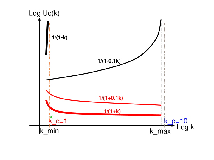
Figure 2: Schematic for $U^{c}(k)=1/(\alpha+c\beta k)$: $0<k_{min}\lesssim k_{c}=1$ and $k_{max}\gg k_{c}$. When $\alpha/\beta=1/0.1$ (thinner lines), the negative chiral sector pole $k_{p}=10\gtrsim k_{max}$. This pole approaches $k_{c}$ when $\alpha/\beta\to 1/1$ (thicker lines) and most of the energy is concentrated at the negative chiral sector around the pole $k_{p}\to k_{c}=1$, the very small wavenumber compared to $k_{max}$: $k_{c}$ is the maximum wavenumber of the positive chiral sector, so the (dominant) positive helicity has opposite sign to the larger-wavenumber modes where injection is supposed be placed in the turbulence simulations of Refs. [25, 26].

As sketched in Fig. 2, we found from the chirally decomposed energy absolute equilibrium spectrum of the full 3D3C system, $U^{c}(k)=1/(\alpha+c\beta k)$, that, if one chiral sector (say, that of ‘$c=+$’ for purely helical modes with positive definite helicity) is truncated to be in between $k_{min}$ and $k_{max}$, and the other ‘alien’ sector in between $k_{min}$ and $k_{c}$ ($\ll k_{max}$), then the ‘alien(s)’ can carry most of the energy when $\alpha/\beta\downarrow k_{c}^{+}$ (with the pole $k_{p}$ approaching $k_{c}$ from above), especially when $k_{c}$ is close to $k_{min}$. Of course, this result also applies to the system in a rotating frame. And, more fascinatingly, if we keep the positive and negative sectors in this fashion for a turbulence system with dissipation at large $k$ and injection at some $k_{in}$ inbetween $k_{min}$ and $k_{max}$, then the indication for large scale behavior and nonlocal transfers (see details in Ref. [24]) is very similar to Mininni et al.’s observations [25, 26], except for one thing (see below), at least.

To be more definite, Mininni at al.[25] stated “… the direct transfer of energy at small scales is mediated by interactions with the largest scale in the system, the energy containing eddies with $k_{\perp}\approx 1$, where $k_{\perp}$ refers to wavevectors perpendicular the axis of rotation. … The inverse transfer of energy at scales larger than the energy injection scale is non-local, and energy is transferred directly from small scales to the largest available scale”, which are basically the same as our prediction from the special truncation scheme in §2.2.2 of Ref. [24], word by word (if we appropriately choose the directions of the wavevector and the corresponding helical mode of the alien(s)); what’s more, Mininni and Pouquet[26] found the “the development of an inverse transfer of energy now coexisting with direct cascades of energy and helicity”. One probably then would guess that the imposed rotation work to naturally depress those modes that are cleanly truncated in the special scheme, which however appears somewhat strange. More seriously, there is no evidence from these simulations that the largest scale is ‘OCSDS’ (one chiral sector dominated state) with chirality opposite to the input (as predicted from the above special absolute equilibrium). We then believed that the inverse energy transfer in rotating turbulence probably had not much to do with the helical energy condensations found in §2.2.2 of Ref. [24]; in other words, the absolute equilibrium sketched in Fig. 2 should not be as relevant to rotating flows as that in Fig. 1. It was nevertheless hoped that such analysis could promote relevant numerical analysis in the fashion of Brandenburg et al. [64] and/or Biferale et al.[62], but looking into the contributions to the spectral transfers functions from the purely helical modes.

Thus, we turned to deal with three separated subsystems, i.e., the 2D $u_{x}$-$u_{y}$ field (S2) with $\partial_{z}\equiv 0$, which conserves energy and enstrophy, the passive scalar $u_{z}$ field (S1 with scalar energy conserved) with $\partial_{z}=0$ advected by S2, and the left 3D field (S3, conserving energy and helicity) with $\partial_{z}$ not vanishing everywhere. We can have the normal energy-helicity AE (absolute equilibrium) of S3 indicating forward energy and helicity cascades; S2 is already discussed by Kraichnan[34], indicating inverse-energy and forward-enstrophy cascades; S1 by itself, without coupling to S2, presents equipartition of the AE energy, indicating forward energy cascade. Note that $S1\oplus S2$, the combination, also conserves helicity on the slow-mode manifold, facilitating energy-enstrophy-helicity AE. The indications of S2 and S3 AEs are consistent with the two-dimensionalization and forward-energy-and-helicity-cascade scenarios as all simulations and observations seem to agree. 2D-3D vortex-wave interaction may be termed re-coupling of S2 and S3, which raises the complex issue of the validity of time regime of the resonant wave theory, for given $Ro$, among other relaxation time scale problems. When resonant wave theory breaks down, we may consider $S1\oplus S2\oplus S3$, i.e., the whole system, energy-helicity AE, which then raises the curious question about the difference between such a state and those of non-rotating ones in §2.2 of Ref. [24]. Thus the problem can be extremely complicated depending on the physical parameters ($Ro$ and $Re$ etc.) and time regimes. Such remarks about absolute equilibria of subsystems of rotating fluid models may also apply to those of 3D gyrokinetics, among others, with fast wave dynamics and slow modes such as zonal flows in nature (say, planet Jupiter) or laboratory such as the tokamak [65]. Indeed, (partial) anisotropization is common to many typical systems and unified treatments, as tried by Cambon and Godeferd [55], may be possible.

References

- [1] B. Favier, F. S. Godeferd, C. Cambon, A. Delache and W. J. T. Bos, Quasi-static magnetohydrodynamic turbulence at high Reynolds number. J. Fluid Mech. 681, 434 (2011).
- [2] C. Cambon, Homogeneous MHD turbulence at weak magnetic Reynolds numbers: approach to angular-dependent spectra. In Advances in Turbulence Studies: Progress in Astronautics and Aeronautics (ed. H. Branover & Y. Unger), vol. 149, pp. 131-145. AIAA(1990).
- [3] H. K. Moffatt, On the suppression of turbulence by a uniform magnetic field. J. Fluid Mech. 28, 571-592 (1967).
- [4] L. M. Smith, J. L. Chasnov and F. Waleffe, Crossover from Two- to Three-Dimensional Turbulence. Phys. Rev. Lett. 77, 2467 (1996).
- [5] A. Celani, S. Musacchio and D. Vincenzi, Turbulence in More than Two and Less than Three Dimensions. Phys. Rev. Lett. 104, 184506 (2010).
- [6] D. Montgomery & L. Turner, Anisotropic magnetohydrodynamic turbulence in a strong external magnetic field. Phys. Fluids 24, 825 (1981).
- [7] H. K. Moffatt, The degree of knottedness of tangled vortex lines. J. Fluid Mech. 35, 117-129 (1969).
- [8] R. H. Kraichnan, Helical turbulence and absolute equilibrium. J. Fluid Mech. 59, 745–752 (1973).
- [9] A. Celani, M. Cencini, A. Mazzino and M. Vergassola, Active and passive fields face to face. New Journal of Physics 6 00 (2004).
- [10] G. Falkovich, K. Gawȩdzki & M. Vergasolla, Particles and fields in fluid turbulence. Rev. Mod. Phys. 73, 913–975 (2001).
- [11] R. H. Kraichnan, Small-Scale Structure of a Scalar Field Convected by Turbulence. Phys. Fluids 11, 945–953 (1968).
- [12] D. Fyfe and D. Montgomery, Inverse cascade of magnetic potential in 2D magnetohydrodynamics. J. Plasma Phys. 16, 181 (1976).
- [13] M. Holzer & E. D. Siggia, Turbulent mixing of a passive scalar. Phys. Fluids 6, 1820–1837 (1994).
- [14] A. Newell, Rossby wave packet interactions. J. Fluid Mech. 35, 255-271 (1969).
- [15] Q. N. Chen, S. Chen, G. L. Eyink & D. Holm, Resonant interactions in rotating homogeneous three-dimensional turbulence. J. Fluid Mech. 542, 139–163 (2005).
- [16] C. Cambon, R. Rubinstein and F. S. Godeferd, Advances in wave turbulence: rapidly rotating flows. New J. Phys. 6, 73 (2004).
- [17] L. M. Smith and Y. Lee, On near resonances and symmetry breaking in forced rotating flows at moderate Rossby number. J. Fluid Mech. 535, 111 (2005).
- [18] C. Cambon and L. Jacquin, Spectral approach to non-isotropic turbulence subjected to rotation. J. Fluid. Mech. 202, 295-317 (1989).
- [19] C. Cambon, N. N. Mansour and F. S. Godeferd, Energy transfer in rotating turbulence. J. Fluid. Mech. 337, 303 - 332 (1997).
- [20] L. Bourouiba and P. Bartello, The intermediate Rossby number range and two-dimensional?Cthree-dimensional transfers in rotating decaying homogeneous turbulence. J. Fluid Mech. 587, 139 - 161 (2007).
- [21] L. Bourouiba, Discreteness and resolution effects in rapidly rotating turbulence. Phys. Rev. E 78, 056309 (2008).
- [22] L. Bourouiba, D. N. Strauba, M. L. Waite, Non-local energy transfers in rotating turbulence at intermediate Rossby number. J. Fluid Mech. 690, 129–147 (2012).
- [23] L. Smith and F. Waleffe, Transfer of energy to two-dimensional large scales in forced, rotating three-dimensional turbulence. Phys. Fluids 11, 1608 - 1622 (1999).
- [24] J.-Z. Zhu, W. Yang & G.-Y. Zhu, Purely helical absolute equilibria and chirality of (magneto)fluid turbulence. J. Fluid. Mech. 739, 479–501 (2014).
- [25] P. D. Mininni, A. Alexakis, and A. Pouquet, Scale interactions and scaling laws in rotating flows at moderate Rossby numbers and large Reynolds numbers. Phys. Fluids 21, 015108 (2009)
- [26] P. D. Mininni and A. Pouquet, Rotating helical turbulence. Part I. Global evolution and spectral behavior. Phys. Fluids 22, 035105 (2010).
- [27] S. Chandrasekhar, Hydrodynamic and hydromagnetic stability. Oxford University Press (1961).
- [28] T.-D. Lee, On some statistical properties of hydrodynamic and hydromagnetic fields. Q. Appl. Math. 10, 69–74 (1952).
- [29] E. Hopf, Statistical hydromechanics and functional calculus, Ratl. Mech. Anal. 1, 87-123 (1952).
- [30] H. K. Moffatt, Note on the triad interactions of homogeneous turbulence. J. Fluid Mech. 741, R3 (2014).
- [31] S. A. Orszag, Statistical Theory of Turbulence, in Fluid Dynamics, Les Houches 1973, 237-374, eds. R. Balian & J.L. Peube. Gordon and Breach, New York (1977).
- [32] J. Lee, Dynamical behavior of the fundamental triadic-interaction system in three dimensional homogeneous turbulence. Phys. Fluids. 22, 40–53 (1979).
- [33] J.-Z. Zhu, Generic 3D solenoidal modes with vanishing quadratic/nonlinear terms, submitted for publication (2015).
- [34] R. H. Kraichnan, Inertial ranges in two-dimensional turbulence. Phys. Fluids 102, 1417–1423 (1967).
- [35] U. Frisch, A. Pomyalov, I. Procaccia and S. Ray, Turbulence in noninteger dimensions by fractal Fourier decimation. Phys. Rev. Lett. 108 074501 (2012)
- [36] J.-Z. Zhu, Note on specific chiral ensembles of statistical hydrodynamics: “Order function” for transition of turbulence transfer scenarios. Phys. Fluids 26, 055109 (2014).
- [37] Z.-S. She and E. Jackson, Constrained Euler System for Navier-Stokes Turbulence. Phys. Rev. Lett. 70, 1255 (1993).
- [38] G. Gallavotti, Nonequilibirum and irreversibility. Springer International Publishing (2014).
- [39] J.-Z. Zhu, Isotropic polarization of compressible flows. J. Fluid Mech., 787 440 (2016)
- [40] A. Celani, A. Lanotte, A. Mazzino & M. Vergassola, Universality and saturation of intermittency in passive scalar turbulence. Phys. Rev. Lett. 84, 2385–2388 (2000).
- [41] L. Bourouiba, Model of a truncated fast rotating flow at infinite Reynolds number. Phys. Fluid 20, 07512 (2008).
- [42] Y. Yamazaki, Y. Kaneda & R. Rubinstein, Dynamics of inviscid truncated model of rotating turbulence. J. Phys. Soc. Jpn. 71, 81 (2002).
- [43] J.-P. Eckmann and D. Ruelle, Ergodic theory of chaos and strange attractors. Rev. Mod. Phys. 57, 617 - 656 (1985). The caveat is that the (Gibbs) measure may be ergodic for the projections onto the space and onto the space, but not in the manifold, constrained by and other invariants, in the whole phase - space: Such partial-ergodicity presents constraint on but not on . Note also that as pointed out By G. L. Eyink and H. Spohn [“Negative-temperature states and large-scale, long-lived vortices in two-dimensional turbulence.” J. Stat. Phys. 70, 833 - 886 (1993)], strict ergodicity is not as easily satisfied but is neither necessary condition to justify equilibrium statistics.
- [44] G. L. Eyink, Dissipative anomalies in singular Euler flows. Phys. D 237, 1956-1968 (2008).
- [45] P. L. Sulem and U. Frisch, Bounds on energy flux for finite energy turbulence. J. Fluid Mech. 72, 417-423 (1975).
- [46] A. Celani, T. Matsumoto, A. Mazzino and M. Vergassola, Scaling and universality in turbulent convection. Phys. Rev. Lett. 88 054503 (2002).
- [47] A. Celani, M. Cencini, A. Mazzino and M. Vergassola, Active vs passive scalar turbulence. Phys. Rev. Lett. 89 234502 (2002).
- [48] E.A. Novikov, Functionals and the method of random forces in turbulence theory, Zh. Exper. Teor. Fiz. 47, 1919-1926 (1964).
- [49] G. Eyink, E. Vishniac, C. Lalescu, H. Aluie, K. Kanov, K. Bürger, R. Burns, C. Meneveau and A. Szalay, Flux-freezing breakdown in high-conductivity magnetohydrodynamic turbulence. Nature 497, 466 (2013).
- [50] U. Frisch and B. Villone, Cauchy’s almost forgotten Lagrangian formulation of the Euler equation for 3D incompressible flow. arXiv:1402.4957v3.
- [51] G. L. Eyink, Stochastic line motion and stochastic flux conservation for nonideal hydromagnetic models. J. Math. Phys. 50, 083102 (2009).
- [52] U. Frisch and A. Wirth, Intermittency of passive scalars in delta-correlated flow: Introduction to recent work. Lecture Notes in Physics 491, 53 – 64 (1997).
- [53] P. R. Kramer, A. Majda and E. Vanden-Eijden, Closure Approximations for Passive Scalar Turbulence: A Comparative Study on an Exactly Solvable Model with Complex Features. Journal of Statistical Physics 111, 565 (2003).
- [54] F. Waleffe, The nature of triad interactions in homogeneous turbulence. Phys. Fluids A 4, 350–363 (1992).
- [55] C. Cambon and F. S. Godeferd, Inertial transfers in freely decaying rotating, stably stratified, and MHD turbulence. In Progress in Turbulence Research: Progress in Astronautics and Aeronautics (ed. H. Branover & Y. Unger), AIAA 162, 150-168 (1993).
- [56] F. Waleffe, Inertial transfers in the helical decomposition. Phys. Fluids A 5, 677–685 (1993).
- [57] M. Cencini, P. Muratore-Ginaneschi & A. Vulpiani, Nonlinear Superposition of Direct and Inverse Cascades in Two-Dimensional Turbulence Forced at Large and Small Scales. Phys. Rev. Lett. 107, 174502 (2011).
- [58] U. Frisch, S. Kurien, R. Pandit, W. Pauls, S.S. Ray, A. Wirth, and J.-Z. Zhu, Galerkin Truncation, Hyperviscosity and Bottleneck in Turbulence. Phys. Rev. Lett. 101, 144501 (2008).
- [59] J.-Z. Zhu and M. Taylor, Intermittency and Thermalization in Turbulence. Chin. Phys. Lett. 27, 054702 (2010).
- [60] J. S. Kain, et al., Some Practical Considerations Regarding Horizontal Resolution in the First Generation of Operational Convection-Allowing NWP. Weather and Forcasting 23, 931 (2008).
- [61] D. Montgomery & L. Turner, Two-and-a-half-dimensional magnetohydrodynamic turbulence. Phys. Fluids 25, 345–349 (1982).
- [62] L. Biferale, S. Musacchio and F. Toschi, Inverse energy cascade in three-dimensional isotropic turbulence. Phys. Rev. Lett. 108 104501 (2012).
- [63] It may make it clearer to quote from Ref. [15] that “the present theorems effectively say nothing about the validity of the resonant wave theory at hight , for realistic values of the Rossby number” and “the asymptotic analysis does not determine the largest possible time” for which theory is proved to be valid.
- [64] A. Brandenburg, W. Dobler & K. Submanian. Magnetic helicity in stellar dynamos: new numerical experiments. Astron. Nachr. 323, 99 - 123 (2002).
- [65] J.-Z. Zhu and G. Hammett, Gyrokinetic absolute equilibrium and turbulence. Phys. Plasmas 17, 122307 - 1 - 13 (2010).
- [66] E. Levich and E. Tzvetkov, Helical cyclogenesis, Phys. Rep. 100A, 53 (1984).
- [67] G. V. Levina and M. T. Montgomery, Numerical Diagnosis of Tropical Cycolgenesis Based on a Hypothesis of Helical Self-Organization of Moist Convective Atmospheric Turbulence. Doklady Earth Sciences 458, 1143 (2014).
- [68] P. Constantin and A. Majda, The Beltrami Spectrum for Incompressible Fluid Flows. Commun. Math. Phys. 115, 435 (1988).
- [69] G. Gallavotti and E. G. D. Cohen, Dynamical ensembles in nonequilibrium statistical mechanics. Phys. Rev. Lett. 74, 2694 (1995).
- [70] H. E. Moses, Eigenfunctions of the curl operator, rotationally invariant Helmholtz theorem and applications to electromagnetic theory and fluid mechanics. SIAM (Soc. Ind. Appl. Math.) J. Appl. Math. 21, 114 (1971).