The gradient flow of the Dirac spectrum

Abstract

We construct chiral perturbation theory for the gradient flow of the microscopic Dirac eigenvalues and compute the density of and correlations between the microscopic eigenvalues at zero and non-zero flow time. The results show that the repulsion of the microscopic Dirac eigenvalues from the dynamical quark mass decreases with increasing gradient flow time. Furthermore, the flow of the spectral resolvent is compared to the flow of the chiral condensate obtained from a fermionic gradient flow.

1 Introduction

The phenomelogical success of Lattice QCD relies on a continuum extrapolation which is consistent with the renormalization properties of the strong interactions. To reduce the ultraviolet quantum fluctuations and to improve the continuum extrapolation, it is not uncommon to smoothen the gauge field configurations on the scale of several lattice spacings. Recently the gradient flow luscher-1 ; luscher-2 ; luscher-weisz ; luscher-chiral has provided new methods to determine renormalized quantities on the lattice, see for example Suzuki ; DelDPR ; RS ; Daniel . The extension of the gradient flow to include the flow of the quark fields luscher-chiral , raises a natural question: To which extend does gradient flow preserve the dynamical properties induced by the fermion determinant? As a first step towards a complete answer we compute in this paper the effect of gradient flow on the microscopic eigenvalues of the Dirac operator. In a standard dynamical simulation the fermion determinant induces an eigenvalue repulsion from the quark mass which increases for decreasing quark mass. This affects the microscopic eigenvalue density in a universal way DN ; WGW ; DOTV which has been verified by lattice simulations with dynamical quarks BerbenniBitsch:1998sy ; Damgaard:2000qt ; Fukaya . The microscopic eigenvalue density at nonzero gradient flow time, computed here, gives the flow time scale for which the microscopic correlations induced by the fermion determinant persist.

Ideally, we would like to see that the large eigenvalues of the Dirac operator flow beyond the ultraviolet cut-off so that they do not contribute to the chiral condensate, while the small eigenvalues remain invariant under the flow such that their dynamical properties stay intact. From the calculation of the chiral condensate luscher-chiral ; BG ; shindler one might think that the flow only affects the low-lying eigenvalues by a trivial rescaling. In practice, the situation will be more complicated: We will show that gradient flow decorrelates the microscopic eigenvalues of the Dirac operator from the eigenvalues at zero flow time. In particular, the microscopic spectral density evolves from the universal form for dynamical quarks, which includes the correlations induced by the fermion determinant, to the quenched spectral density. This transition occurs for flow times of order $1/\sqrt{V}$, where a new low energy constant makes the dimensions match.

All results will be obtained from the chiral Lagrangian for the generating function of the Dirac spectrum in the $\epsilon$-domain of QCD. This generating function has dynamical quarks at zero flow time while the valence quarks are at non-zero flow time. The resulting flavor symmetry breaking in the generating function gives rise to a non-trivial $t-$dependence of the chiral Lagrangian for gradient flow. As we will explain in detail, this explicit $t$-dependence is distinct from that of the chiral Lagrangian for the fermonic flow discussed in BG .

Both the chiral condensate as defined through the fermonic flow and the spectral resolvent, evaluated at the dynamical quark mass, evolve from the chiral condensate at zero flow time. The evolution of the two is however different. We explicitly compute and compare the two at non-zero flow time.

The outline of this paper is as follows. In section 2 we give a basic review of gradient flow. Chiral perturbation theory including the chiral Lagrangian in the $\epsilon$-domain is discussed in section 3. Explicit results of the flow of the one-flavor and quenched Dirac spectrum are evaluated in section 4. Concluding remarks are made in section 5, and additional technical details are worked out in the Appendix.

2 The flow equations

A fully dynamical lattice simulation of the strong interactions provides an ensemble of gauge field configurations, $A_{\mu}$, that includes correlations induced by the fermion determinant. As a way to reduce the ultraviolet fluctuations of these configurations one may consider instead the flow time ($t$) dependent gauge fields $B_{\mu}(t,x)$ introduced in luscher-1 . They evolve from the conventional gauge fields $A_{\mu}(x)$ through initial conditions $A_{\mu}(x)=B_{\mu}(0,x)$ and satisfy the first order differential equation

$$\partial_{t}B_{\mu}=D_{\nu}G_{\mu\nu}\,,$$ (1)

where $G_{\mu\nu}$ is the field strength tensor

$$G_{\mu\nu}=\partial_{\mu}B_{\nu}-\partial_{\nu}B_{\mu}+[B_{\mu},B_{\nu}]\,,$$ (2)

and $D_{\mu}=\partial_{\mu}+[B_{\mu},\cdot\,]$ is the covariant derivative. Note that the gauge field flow is determined by the gradient of the Yang-Mills action and that the flow time has dimension of $L^{2}$ luscher-1 . One may also introduce the quark field $\chi(t,x)$ and anti-quark field $\bar{\chi}(t,x)$ which flow according to luscher-chiral

$$\partial_{t}\chi=\Delta\chi\,,\quad\partial_{t}\bar{\chi}=\bar{\chi}\reflectbox{$\vec{\reflectbox{$\Delta$}}$}\,,$$ (3)

where $\Delta=(\partial_{\mu}+B_{\mu})(\partial_{\mu}+B_{\mu})$ is the covariant Laplacian. The initial conditions $\psi(x)=\chi(0,x)$ and $\bar{\psi}(x)=\bar{\chi}(0,x)$ relate the flow time dependent quark fields to the dynamical quark fields in the simulation at zero flow time.

In the above differential equations the quark fields at non-zero flow time do not enter the gauge field flow. Initially, at $t=0$, the quarks and gluons are dynamical, but at non-zero $t$ the gauge field flow is independent of the flow of the fermion. The central aim of this paper is to compute the flow of the Dirac eigenvalues and to discuss how the dynamical properties of the eigenvalues and the chiral condensate changes with flow time. In this discussion the central observables are:

1) The chiral condensate as obtained from the fermionic flow

$$\left\langle S^{0}_{t}\right\rangle\equiv\left\langle\bar{\chi}\chi\right\rangle=\frac{1}{Z_{t=0}(m)}\int{\cal D}A_{\mu}{\cal D}\bar{\psi}{\cal D}\psi\;\bar{\chi}\chi\;e^{\bar{\psi}(D(A_{\mu})+m)\psi-S_{\rm YM}(A_{\mu})},$$ (4)

where $\bar{\chi}$ and $\chi$ are obtained from $\bar{\psi}$, $\psi$ and $A_{\mu}$ through (3) and (1). $D(A_{\mu})$ is the Dirac operator evaluated on the gauge field $A_{\mu}$, $S_{\rm YM}$ is the standard Yang-Mills action and

$$Z_{t=0}(m)=\int{\cal D}A_{\mu}{\cal D}\bar{\psi}{\cal D}\psi\;e^{\bar{\psi}(D(A_{\mu})+m)\psi-S_{\rm YM}(A_{\mu})}.$$ (5)

Note that a new source term at time $t$ must be introduced into the generating function in order to write $\left\langle\bar{\chi}\chi\right\rangle$ as a derivative

$$\left\langle S^{0}_{t}\right\rangle\equiv\left\langle\bar{\chi}\chi\right\rangle=\frac{1}{Z_{t=0}(m)}\lim_{m_{t}\to 0}\frac{d}{dm_{t}}\int{\cal D}A_{\mu}{\cal D}\bar{\psi}{\cal D}\psi\;e^{\bar{\psi}(D(A_{\mu})+m)\psi+m_{t}\bar{\chi}\chi-S_{\rm YM}(A_{\mu})}\,.$$ (6)

2) The second kind of observables we will discuss are resolvents for the Dirac spectrum. In this case there is no gradient flow of the fermion fields and only the flow of the gauge fields is taken into account. The resolvent for the one point function of the Dirac spectrum at flow time $t$ is given by

$$\left\langle{\cal S}^{0}_{t}\right\rangle \equiv \left\langle{\rm Tr}\frac{1}{D(B_{\mu})+m_{v}}\right\rangle$$

$$\equiv \frac{1}{Z_{t=0}(m)}\lim_{\tilde{m}_{v}\to m_{v}}\frac{d}{dm_{v}}\int{\cal D}A_{\mu}\;{{\det}}^{N_{f}}(D(A_{\mu})+m)\frac{{\det}(D(B_{\mu})+m_{v})}{{\det}(D(B_{\mu})+\tilde{m}_{v})}e^{-S_{\rm YM}(A_{\mu})}\,,$$

where $B_{\mu}$ is obtained from $A_{\mu}$ through (1). We discuss similarities and differences between $\left\langle{\cal S}^{0}_{t}\right\rangle$ and $\left\langle S^{0}_{t}\right\rangle$ in section 3.4. The eigenvalue density of $D(B_{\mu})$ will be obtained from $\left\langle{\cal S}^{0}_{t}\right\rangle$ in section 4.1.

The computation of the above observables will be performed within chiral perturbation theory.

3 Chiral Perturbation Theory for Gradient Flow

Chiral perturbation theory at non-zero flow time in the $p$-regime for $\left\langle S^{0}_{t}\right\rangle$ was introduced in BG . After a brief review of these results and the extension thereof to the $\epsilon$-regime we set up chiral perturbation theory for $\left\langle{\cal S}^{0}_{t}\right\rangle$.

3.1 $p$-regime and the generating function for $\left\langle S^{0}_{t}\right\rangle$

To order the terms in the chiral Lagrangian a counting scheme must be adopted. We will start out with the $p$-regime counting

$$\partial_{\mu}\thicksim\frac{1}{L}\thicksim\epsilon\,,\quad\text{and}\quad m\thicksim m_{t}\thicksim\frac{1}{\sqrt{V}}\thicksim\epsilon^{2}\,.$$ (8)

Note that the source $m_{t}$ will be put to zero after differentiation. For the standard $t=0$ partition function (5) the chiral Lagrangian to leading order is simply given by GLorig ; GL

$${\mathcal{L}}=\frac{f^{2}}{4}{\rm Tr}(\partial_{\mu}U\partial_{\mu}U^{\dagger})+\frac{\Sigma}{2}{\rm Tr}({\cal M}U+U^{\dagger}{\cal M})\,,$$ (9)

where $\mathcal{M}=\mathrm{Diag}(m_{1},\ldots,m_{N_{f}})$ is the quark mass matrix, the low energy constant $\Sigma$ is the chiral condensate and $f$ is the pion decay constant. This celebrated chiral Lagrangian describes the non-perturbative low energy phase where the strong interactions spontaneously break chiral symmetry.

The unitary field $U$ is defined as

$$U(x)=\exp\left(\frac{2i\pi^{a}(x)T^{a}}{f}\right)\,,$$ (10)

where $\pi^{a}$ are Goldstone bosons and $T^{a}$ are the generators of the $SU(N_{f})$ flavor group.

The extension of the chiral Lagrangian needed to compute $\langle S^{0}_{t}\rangle=\langle\bar{\chi}\chi\rangle$ at non-zero flow time was written down in BG : As observed above Eq. (6) the generating function for $\langle S^{0}_{t}\rangle$ includes an explicit source term for this observable. Since the chiral transformation properties of $\bar{\chi}$ and $\chi$ are independent of $t$, the spurion properties of the new quark mass source $m_{t}$ will be identical to that of the standard quark mass $m$. Hence, the $m_{t}$ dependent terms in the chiral Lagrangian must be of exactly the same form as the standard mass terms, but the magnitude of the low energy constants appearing in combination with $m_{t}$ can change with $t$. As the counting for $m$ and $m_{t}$ is identical, cf. (8), the new term at leading order must have the same form as the original one BG

$$\mathcal{L}^{\prime}=\frac{m_{t}\Sigma_{t}}{2}{\rm Tr}(U+U^{\dagger})\,,$$ (11)

where we have introduced the low energy constant at flow time $t$, $\Sigma_{t}$. The sum ${\mathcal{L}}+\mathcal{L}^{\prime}$ makes up the lowest order chiral Lagrangian in the generating function for $\langle S^{0}_{t}\rangle$ at leading order in the $p$-regime BG .

Within the $p$-counting the Compton wavelength of the pions is comparable to the dimension of the box $1/M_{\pi}\thicksim L$. Perturbatively, the flow introduces a smearing width of $\sqrt{8t}$ luscher-1 , and it is natural to consider this to be much smaller than $L$ and the Compton wavelength of the pions luscher-chiral ; BG .

3.2 $\epsilon$-regime generating function for $\left\langle S^{0}_{t}\right\rangle$

In this section we set up the $\epsilon$-regime of the generating function for $\left\langle S^{0}_{t}\right\rangle$ at non-zero flow time. The natural extension of the counting in the $\epsilon$-regime is one where the standard mass $m$ and the source mass, $m_{t}$, for $\bar{\chi}\chi$ are of the same order

$$\partial_{\mu}\thicksim\frac{1}{L}\thicksim\epsilon\,,\quad m\thicksim m_{t}\thicksim\frac{1}{V}\thicksim\epsilon^{4}\,.$$ (12)

Also in this case the source $m_{t}$ will be put to zero after differentiation. As in the $p$-regime the flow does not break the chiral symmetries and the form of the possible mass terms in the chiral Lagrangian are identical.

Note that the new low energy parameter $\Sigma_{t}$ evolves with $t$ from the value $\Sigma$ at $t=0$ in a way that is not determined by chiral perturbation theory. In order to keep this constant of order $\epsilon^{0}$ we need to include the new scale set by the smearing width $\sqrt{8t}$ luscher-chiral into the $\epsilon$-counting scheme. As in BG we will consider the case where $\sqrt{8t}$ is smaller than the pion Compton wavelength

$$\sqrt{8t}\ll\frac{1}{M_{\pi}}\,.$$ (13)

In the $\epsilon$-regime, however, this is condition is much less constraining since

$$1/M_{\pi}\thicksim 1/\epsilon^{2}\thicksim L^{2}\ .$$ (14)

For example, it would allow for a smearing width that it is comparable ${\cal O}(1/\epsilon)$ or even larger than the extent of the box. This is, however, undesirable: If we expand the difference between the chiral condensate at zero and non-zero flow time for small $t$ we get BG

$$\Sigma_{t}-\Sigma=(t\Lambda_{\rm QCD}^{2})\sigma_{1}+(t\Lambda_{\rm QCD}^{2})^{2}\sigma_{2}+...\,,$$ (15)

where $\sigma_{1},\sigma_{2},...$ are the Taylor-coefficients. With $\sqrt{8t}\thicksim 1/\epsilon$ (which is allowed by the constraint (13)) this would imply that $\Sigma$ and/or $\Sigma_{t}$ would have to scale at least as fast as $1/\epsilon^{2}$. To keep $\Sigma_{t}$ of order one requires a counting scheme with

$$\sqrt{8t}\thicksim\epsilon^{0}\quad\quad\quad\quad(t\ {\rm counting\ for}\ \left\langle S^{0}_{t}\right\rangle).$$ (16)

Having settled the counting we can now write down the form of the effective theory for the generating function Eq. (6).

In the $\epsilon$-regime the zero modes of the Goldstone field dominate the partition function and the kinetic term in (9) factorizes from the partition function GL . At leading order in the $\epsilon$-counting the effective generating function of $\left\langle S^{0}_{t}\right\rangle$ is hence is given by the group integral

$$\mathcal{Z}_{N_{f}} = \int\limits_{U(N_{f})}\mathcal{D}U\ {{\det}}^{\nu}(U)\exp\left(\frac{\Sigma V}{2}{\rm Tr}\left[\mathcal{M}U+U^{-1}\mathcal{M}\right]+\frac{m_{t}\Sigma_{t}V}{2}{\rm Tr}\left[U+U^{-1}\right]\right),$$

where $V$ is the four volume. The integration is over $U(N_{f})$ since we consider the sector with fixed topological index $\nu$ LS . Note that the $t$-dependence enters through the undetermined flow time dependent low energy parameter, $\Sigma_{t}$, and that $\sqrt{8t}\thicksim\epsilon^{0}$. (For $t\thicksim\epsilon$ one may replace $\Sigma_{t}$ by $\Sigma$ in (LABEL:Zgen-chibarchi), since the difference between the two will be of order $\epsilon$ acceding to (15).)

Let us now turn to the effective generating function for the spectral resolvent of Eq. (2). The presence of determinants at different flow times presents a new situation not faced in BG .

3.3 $\epsilon$-regime generating function for $\left\langle{\cal S}^{0}_{t}\right\rangle$

In this section we construct the low energy generating function for the spectral resolvent $\left\langle{\cal S}^{0}_{t}\right\rangle$. For simplicity consider one dynamical flavor where the generating function for $\left\langle{\cal S}^{0}_{t}\right\rangle$ is given by

$$\int{\cal D}A_{\mu}\,{\det}(D(A_{\mu})+m)\frac{{\det}(D(B_{\mu})+m_{v})}{{\det}(D(B_{\mu})+\tilde{m}_{v})}\,e^{-S_{\rm YM}(A_{\mu})}$$ (25)

$$= \int{\cal D}\bar{\psi}{\cal D}\psi{\cal D}\bar{\eta}_{f}{\cal D}\eta_{f}{\cal D}\bar{\eta}_{b}{\cal D}\eta_{b}{\cal D}A_{\mu}\,e^{-S_{\rm YM}(A_{\mu})}\;$$

$$\hskip 28.45274pt\times\exp\left[(\bar{\psi}\ \bar{\eta}_{f}\ \bar{\eta}_{b})\left(\begin{array}[]{ccc}D(A_{\mu})+m&0&0\\ 0&D(B_{\mu})+m_{v}&0\\ 0&0&D(B_{\mu})+\tilde{m}_{v}\end{array}\right)\left(\begin{array}[]{c}\psi\\ \eta_{f}\\ \eta_{b}\end{array}\right)\right].$$

We stress that the gauge fields $B_{\mu}$ are obtained from (1) using the dynamical gauge field $A_{\mu}$ as initial condition while the $\eta$ fields are valence quarks. Note also that $\eta_{b}$ and $\bar{\eta}_{b}$ obey bosonic statistics.

Since the Dirac operators are not defined for the same gauge field configurations the flavor symmetries are violated even at vanishing quark masses. The difference between the Dirac operators leads to a new term of the form

$$\gamma_{\mu}(B_{\mu}-A_{\mu}){\rm Diag}(0,1,1).$$ (26)

Note that this is not an external source term, $B_{\mu}$ depends on $A_{\mu}$ and will be integrated out along with it.

With infinitesimal $t$ we have that cf. (1)

$$B_{\mu}-A_{\mu}=D_{\nu}F_{\mu\nu}t\,,$$ (27)

where $F_{\mu\nu}$ is the field strength at $t=0$ and $D_{\mu}$ likewise is evaluated at $t=0$. Hence, the new term in the generating function for small $t$ is

$$\bar{\Psi}\;t\;{\rm Diag}(0,1,1)\gamma_{\mu}D_{\nu}F_{\mu\nu}\;\Psi,$$ (28)

where

$$\Psi=\left(\begin{array}[]{c}\psi\\ \eta_{f}\\ \eta_{b}\end{array}\right).$$ (32)

The new term, (28), breaks the flavor symmetries as a vector source (this linearized breaking is sufficient as we will work to leading order in $t$). Hence, in the chiral Lagrangian for the generating function we must include all possible terms which break the symmetries in this manner. To identify these terms we promote $t$ to a spurion field which transforms such that (28) is invariant. In the chiral Lagrangian theory we then include all the possible invariant terms including the spurion $t$. The possible terms with at most two $t$’s are

$${\rm Str}\left[tU^{-1}tU\right],\quad{\rm Str}\left[tt\right]\quad{\rm and}\quad i{\rm Str}\left[t_{\mu}U^{-1}\partial_{\mu}U-t_{\mu}(\partial_{\mu}U^{-1})U\right],$$ (33)

with $t_{\mu}=t$.

To obtain the leading terms in the chiral Lagrangian we need to define a counting scheme. We will adopt $t$ into the $\epsilon$-counting such that

$$\partial_{\mu}\thicksim\frac{1}{L}\thicksim\epsilon\,,\quad\text{and}\quad m\thicksim m_{v}\thicksim\frac{1}{V}\thicksim\epsilon^{4}\quad\text{and}\quad t\thicksim\frac{1}{L^{2}}\thicksim\epsilon^{2}$$

$$\quad\quad\quad\quad\quad\quad\quad\quad(t\ {\rm counting\ for}\ \left\langle{\cal S}^{0}_{t}\right\rangle)\,.$$ (34)

Note that the counting for $t$ is different from that in the generating function for $\left\langle S^{0}_{t}\right\rangle$. Then to leading order we have the low energy generating function

$${\cal Z}_{N_{f}+1|1}(m,m_{v}|\tilde{m}_{v})$$

$$= \int\limits_{Gl(N_{f}+1|1)}\mathcal{D}U\ {{\rm Sdet}}^{\nu}U\exp\left(\frac{1}{2}{\rm Str}\left[\mathcal{M}U+U^{-1}\mathcal{M}\right]+t^{2}F_{\rm flow}^{2}V{\rm Str}\left[{\cal T}U^{-1}{\cal T}U\right]\right)\,,$$

where $\mathcal{M}=\mathrm{Diag}(\overbrace{m\Sigma V,\ldots,m\Sigma V}^{N_{f}},m_{v}\Sigma V,\tilde{m}_{v}\Sigma V)$ and ${\cal T}={\rm Diag}(\overbrace{0,\ldots,0}^{N_{f}},1,1)$.

The condensate $\Sigma$ that multiplies $m_{v}$ differs from the condensate at $t=0$ by terms of $O(t)$ which do not contribute to leading order in the $\epsilon$ counting. The new low energy constant $F_{\rm flow}$ depends on the details of the flow. Other flow equations for $B_{\mu}$ which break the symmetries of the generating functional in the same manner as the flow considered here, will correspond to different values of $F_{\rm flow}$. Note that $F_{\rm flow}$ has dimension 4 such that $t^{2}F_{\rm flow}^{2}V$ is dimensionless.

3.4 The similarities and differences between $\langle S^{0}_{t}\rangle$ and $\langle{\cal S}^{0}_{t}\rangle$

Since $\langle S^{0}_{t}\rangle$ and $\langle{\cal S}^{0}_{t}\rangle$ (evaluated at the physical quark mass) both evolve from $\langle\bar{\psi}\psi\rangle$ at zero flow time one may potentially use either to define the chiral condensate at non-zero flow time. While $\langle S^{0}_{t}\rangle$ is defined through the flow of the fermions $\langle{\cal S}^{0}_{t}\rangle$ depends only on the gradient flow of the gauge fields. The two are therefore not necessarily equal at nonzero flow time. To compare the two quantitatively we here discuss their exact form in the $\epsilon$-regime.

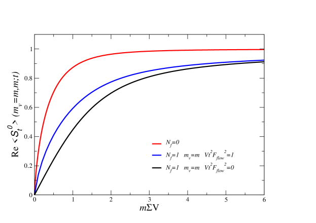
Figure 1: The real part of the spectral resolvent at flow time $F_{\rm flow}^{2}t^{2}V=1$ (middle curve) evaluated at the valence mass equal to the dynamical mass, $m_{v}=m$, and plotted as a function of $m\Sigma V$. At $t=0$ the result (lower curve) matched the fully dynamical microscopic eigenvalue density while the quenched condensate (upper curve) is approached for large flow time $F_{\rm flow}^{2}t^{2}V\gg 1$.

In the $\epsilon$-regime the condensate from the fermonic flow, $\langle S^{0}_{t}\rangle$, follows from (LABEL:Zgen-chibarchi) by evaluating the derivative wrt. $m_{t}$ of $\log Z$ at $m_{t}=0$. From (LABEL:Zgen-chibarchi) it is clear this expression takes the same form as the standard chiral condensate at $t=0$, only the overall scale is now set by the flow time dependent low energy parameter $\Sigma_{t}$. For $N_{f}=1$ the result is

$$\langle S^{0}_{t}\rangle=\Sigma_{t}\frac{1}{2}\frac{I_{\nu+1}(m\Sigma V)+I_{\nu-1}(m\Sigma V)}{I_{\nu}(m\Sigma V)}\ .$$ (36)

Note that the $t$ dependence of $\Sigma_{t}$ is not determined by chiral perturbation theory.

To determine $\left\langle{\cal S}_{t}^{0}\right\rangle$ for $N_{f}=1$ in the $\epsilon$-regime we make use of an explicit parametrization of $Gl(2|1)$ in the generating function (3.3). The parametrization and details are given in Appendix A. A plot of $\left\langle{\cal S}_{t}^{0}\right\rangle$ evaluated at the valence quark mass, $m_{v}$, equal to the physical quark mass, $m$, as a function of $mV\Sigma$ is shown in Fig. 1. Initially, at zero flow time, $\left\langle{\cal S}_{t}^{0}\right\rangle$ is the dynamical condensate which includes the full effect of the fermion determinant. With increasing flow time $\left\langle{\cal S}_{t}^{0}\right\rangle_{m_{v}=m}$ approaches the quenched form which it reaches in the limit $t^{2}F_{\rm flow}^{2}V\gg 1$.

4 Dirac spectra

Let us now turn to the flow of the Dirac spectra. At zero flow time the eigenvalues of the Dirac operator are determined by the eigenvalue equation

$$D(A_{\mu})\psi^{A}_{n}=i\lambda^{A}_{n}\psi^{A}_{n}\,.$$ (37)

As the gauge field $B_{\mu}$ evolves with the flow according to (1) from its initial value $A_{\mu}$, the eigenvalues of the Dirac operator evaluated on $B_{\mu}$ are given by

$$D(B_{\mu})\psi^{B}_{n}=i\lambda^{B}_{n}\psi^{B}_{n}\,.$$ (38)

Here we will compute the microscopic eigenvalue density at time $t$ as well as the two point function between the spectra at time $t=0$ and at time $t$.

4.1 The spectral one point function in the $\epsilon$-regime

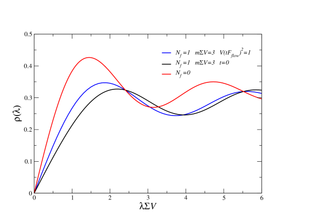
Figure 2: The microscopic eigenvalue density for zero topological charge at non-zero flow time $t$. As the flow proceeds the microscopic eigenvalue density smoothly moves from the fully dynamical result (at $t=0$) to the quenched form at $F_{\rm flow}^{2}t^{2}V\gg 1$. In the plot the dynamical quark mass is $m\Sigma V=3$ and the flow time is chosen such that $F_{\rm flow}^{2}t^{2}V=1$.

Since $\langle{\cal S}_{t}^{0}\rangle$ is the partially quenched condensate, the eigenvalue density of $D(B_{\mu})$ is simply the discontinuity of $\langle{\cal S}_{t}^{0}\rangle$ across the imaginary axis

$$\rho_{t}(\lambda^{B},m) = \lim_{\epsilon\to 0}\frac{1}{\pi}\left(\left\langle{\rm Tr}\frac{1}{D(B_{\mu})+i\lambda^{B}+\epsilon}\right\rangle-\left\langle{\rm Tr}\frac{1}{D(B_{\mu})+i\lambda^{B}-\epsilon}\right\rangle\right)$$

$$= \lim_{\epsilon\to 0}\left(\left\langle{\cal S}_{t}^{0}\right\rangle_{m_{v}=i\lambda^{B}+\epsilon}-\left\langle{\cal S}_{t}^{0}\right\rangle_{m_{v}=i\lambda^{B}-\epsilon}\right).$$

Let us first consider the quenched case. In this case the generating function, (25), for $\left\langle{\cal S}_{t}^{0}\right\rangle$ only involves the valence quarks. Both of these appear together with $D(B_{\mu})$ and the evolution of the gauge field therefore does not break the flavor symmetries of the generating function. The $t^{2}$ term in the effective generating function is therefore absent. This also follows directly from (3.3) by observing that the ${\cal T}$ matrix for $N_{f}=0$ is proportional to unity, resulting in

$${\rm Str}[U{\cal T}U^{-1}{\cal T}]\propto{\rm Str}[UU^{-1}]={\rm Str}[{\mathbb{1}}]=0\quad\quad\quad(N_{f}=0).$$ (40)

We conclude that the quenched microscopic eigenvalue density is independent of the flow time, and in the sector of topological charge $\nu$ it is given by VZ

$$\rho_{N_{f}=0}(\lambda^{B}\Sigma V)=\frac{1}{2}\lambda^{B}\Sigma V\left[J_{\nu}^{2}(\lambda^{B}\Sigma V)-J_{\nu-1}(\lambda^{B}\Sigma V)J_{\nu+1}(\lambda^{B}\Sigma V)\right]+\nu\delta(\lambda^{B}\Sigma V).$$

The unquenched eigenvalue density of $D(B_{\mu})$ depends on time as the ${\cal T}$ matrix is non-trivial. To obtain the unquenched eigenvalue density we only need to put $m_{v}=i\lambda^{B}$ and take the real part of $\langle{\cal S}_{t}^{0}\rangle$ calculated in Appendix A for $N_{f}=1$. The resulting eigenvalue density is plotted in Fig. 2 for $VF_{\rm flow}^{2}t^{2}=1$ and $m\Sigma V=3$. Also shown is the fully dynamical $t=0$ result as well as the quenched spectral density. At small $\lambda\Sigma V$ the fully dynamical eigenvalue density falls below the quenched curve due to the repulsion of the smallest eigenvalues from the dynamical quarks mass. The curve for $VF_{\rm flow}^{2}t^{2}=1$ shows how this repulsion is reduced by the flow such that at $VF_{\rm flow}^{2}t^{2}\gg 1$ the microscopic eigenvalue density takes the quenched form (recall that the new low energy constant $F_{\rm flow}$ has dimension 4 such that $VF_{\rm flow}^{2}t^{2}$ is dimensionless). The flow time scale for the loss of these dynamical correlations is already much earlier at $t\thicksim m_{\pi}f/F_{\rm flow}$. In this manner $F_{\rm flow}$ determines how long the microscopic eigenvalue spectrum maintains its dynamical properties.

Notice also that the number of eigenvalues equal to zero remains unchanged as the time flows. In other words, the index of $D(A_{\mu})$ is equal to that of $D(B_{\mu})$.

4.2 The spectral two-point function in the $\epsilon$-regime

In order to better understand the flow of the eigenvalues of the Dirac operator we will here extend the standard spectral two point function $\rho(\lambda_{1},\lambda_{2})$ (where both eigenvalues are part of the spectrum of the Dirac operator evaluated for $A_{\mu}$ at time $t=0$) to non-zero flow time. We will consider the case where $\lambda_{1}=\lambda^{A}$ is an eigenvalue of $D(A_{\mu})$ at $t=0$ and $\lambda_{2}=\lambda^{B}$ is an eigenvalue of $D(B_{\mu})$ at time $t$. This spectral correlation function is denoted by $\rho(\lambda^{A},\lambda^{B};t)$.

The correlation function between the eigenvalues at zero and non-zero $t$ reads

$$\begin{split}\rho(\lambda^{A},\lambda^{B};t)\equiv&\,\left\langle\sum_{n}\delta(\lambda^{A}-\lambda^{A}_{n})\sum_{m}\delta(\lambda^{B}-\lambda^{B}_{m})\right\rangle\\ &-\left\langle\sum_{n}\delta(\lambda^{A}-\lambda^{A}_{n})\right\rangle\left\langle\sum_{m}\delta(\lambda^{B}-\lambda^{B}_{m})\right\rangle\,.\end{split}$$ (42)

It is related to the susceptibility through

$$\rho(\lambda^{A},\lambda^{B};t)=\frac{1}{4\pi^{2}}{\rm disc}\,\chi(m_{A},m_{B};t)\Big{|}_{\begin{subarray}{c}m_{A}=i\lambda^{A}\\ m_{B}=i\lambda^{B}\end{subarray}}\,,$$ (43)

where

$$\chi(m_{A},m_{B};t)=\left\langle\sum_{n}\frac{1}{i\lambda_{n}^{A}+m_{A}}\sum_{m}\frac{1}{i\lambda_{m}^{B}+m_{B}}\right\rangle-\left\langle\sum_{n}\frac{1}{i\lambda_{n}^{A}+m_{A}}\right\rangle\left\langle\sum_{m}\frac{1}{i\lambda_{m}^{B}+m_{B}}\right\rangle\,.$$ (44)

A similar spectral two point function was used in DHSS ; DHSST ; Damgaard:2006pu to extract the value of the pion decay constant from lattice QCD simulations.

Before performing an exact calculation of the two-point function, let us first give a qualitative discussion of its properties. The two point correlation function satisfies the identities

$$\int\rho(\lambda^{A},\lambda^{B},t)\;d\lambda^{A} = 0,$$

$$\int\rho(\lambda^{A},\lambda^{B},t)\;d\lambda^{B} = 0,$$ (45)

which follow immediately from the normalization

$$\int\sum_{n}\delta(\lambda-\lambda^{A}_{n})\;d\lambda=N$$ (46)

with $N$ equal to the total number of eigenvalues and the corresponding normalization for $\lambda^{B}_{n}$. Let us first discuss the case of $t=0$. Then the first term in (4.6) can be decomposed as

$$\delta(\lambda^{A}-\lambda^{B})\rho(\lambda^{A})+\sum_{n\neq m}\delta(\lambda^{A}-\lambda^{A}_{n})\delta(\lambda^{B}-\lambda^{B}_{m}).$$ (47)

Correlations due to the first term are known as self-correlations, whereas the second term represents the genuine two-point correlations. Because of the sum rule (45) the integral over the genuine two-point correlations is negative with the total negative area equal to the spectral density at $\lambda^{A}$. Since spectral correlations decrease for increasing distance, we expect that the genuine two-point correlation function starts at a negative number and then asymptotes to zero for increasing distance.

At small nonzero flow time, we expect that eigenvalues $\lambda^{B}_{k}$ fluctuate in a Gaussian way about the eigenvalues $\lambda^{A}_{k}$, i.e.

$$\lambda^{B}_{k}=\lambda^{A}_{k}+\delta^{B}_{k}$$ (48)

with the distribution of $\delta^{B}_{k}$ given by

$$P(\delta^{B}_{k})=\frac{1}{\sqrt{2\pi\sigma}}e^{-(\delta^{B}_{k})^{2}/2\sigma^{2}}.$$ (49)

For the self-correlations we now find

$$\int d\delta^{B}_{k}P(\delta^{B}_{k})\left\langle\sum_{k}\delta(\lambda^{A}-\lambda^{A}_{k})\delta(\lambda^{B}-\lambda^{A}_{k}-\delta_{k}^{B})\right\rangle$$

$$=\frac{\rho(\lambda_{A})}{\sqrt{2\pi\sigma}}e^{(\lambda^{A}-\lambda^{B})^{2}/2\sigma^{2}}.$$ (50)

So for the two-point correlation function at small nonzero flow-time, we expect to find a Gaussian peak centered at $\lambda_{A}=\lambda_{B}$ and because of the sum rule (45) a negative correlation gap away from this peak. This is exactly the behavior we will find in the explicit calculation in the next section (see Fig. 3).

4.2.1 Quenched two-point function

In order to compute the spectral two point correlation function we will use a version of the replica method that was introduced in SVtoda . In this approach the replica limit is obtained from a recursion relation for the generating function. We will consider the two-point function in the quenced case $N_{f}=0$.

In replica approach, see eg. rep-sk ; replica ; SVtoda ; Kanzieper , the susceptibility reads

$$\chi(m_{A},m_{B};t)\equiv\lim_{n\to 0}\frac{1}{n^{2}}\partial_{m_{A}}\partial_{m_{B}}\log Z_{n}(m_{A},m_{B};t)\,,$$ (51)

where the replicated generating function is given by

$$Z_{n}(m_{A},m_{B};t)=\int{\cal D}A_{\mu}\,{\det}^{n}(D(A_{\mu})+m_{A})\,{\det}^{n}(D(B_{\mu})+m_{B})\,e^{-S_{\rm YM}(A_{\mu})}\,.$$ (52)

In the low energy effective description (cf. section 3.3) we have

$$Z_{n}(m_{A},m_{B};t)=\int_{U(2n)}{\cal D}U\,{\det}^{\nu}(U)e^{\frac{1}{2}\Sigma V{\rm Tr}({\cal M}^{\dagger}U+{\cal M}U^{\dagger})+VF_{\rm flow}^{2}t^{2}{\rm Tr}({\cal T}U^{\dagger}{\cal T}U)}\,,$$ (53)

with ${\cal M}={\rm Diag}(m_{A},\ldots,m_{A},m_{B},\ldots,m_{B})$ and ${\cal T}={\rm Diag}(0,\ldots,0,1,\ldots,1)$.

In order to compute the low energy replicated generating function we first note that the $U(2n)$ integral changes only by a trivial factor if we shift ${\cal T}$ by the unit matrix since

$${\rm Tr}(({\cal T}-\frac{1}{2}\mathbb{1})U^{\dagger}({\cal T}-{\frac{1}{2}}\mathbb{1})U)={\rm Tr}({\cal T}U^{\dagger}{\cal T}U)-{\rm Tr}({\cal T})+\frac{1}{4}{\rm Tr}\mathbb{1}={\rm Tr}({\cal T}U^{\dagger}{\cal T}U)-\frac{1}{2}n\,.$$

Now using that $({\cal T}-\frac{1}{2}\mathbb{1})=-\frac{1}{2}B$, where $B\equiv{\rm Diag}(\mathbb{1},-\mathbb{1})$, the replicated partition function can be written

$$Z_{n}(m_{A},m_{B};t)=e^{\frac{1}{2}nVF_{\rm flow}^{2}t^{2}}\int_{U(2n)}{\cal D}U\,{\det}^{\nu}(U)e^{\frac{1}{2}\Sigma V{\rm Tr}(M^{\dagger}U+MU^{\dagger})+\frac{1}{4}VF_{\rm flow}^{2}t^{2}{\rm Tr}(BU^{\dagger}BU)}\,.$$ (55)

The integral over $U(2n)$ above is of the same form as the one considered in SVfact ; DHSS , where it was found that the replicated partition function with $2n$ fermions can be expressed in terms of the $n=1$ partition function

$$(m_{A}m_{B})^{n(n-1)}Z_{n}(m_{A},m_{B};t)=D_{n}{\det}\left[(m_{A}\partial_{m_{A}})^{k}(m_{B}\partial_{m_{B}})^{l}Z_{1}(m_{A},m_{B};t)\right]\,,$$ (56)

where $D_{n}$ is a constant to ensure normalization and $k,l=0,1,...,n-1$. Since the above partition function is a $\tau$-function the $Z_{n}$ satisfy the Toda lattice equation DHSS

$$\begin{split}\frac{1}{4n^{2}V^{4}\Sigma^{4}}m_{A}\partial_{m_{A}}m_{B}\partial_{m_{B}}\log Z_{n}&(m_{A},m_{B};t)\\ =&\,(m_{A}m_{B})^{2}\frac{Z_{n+1}(m_{A},m_{B};t)Z_{n-1}(m_{A},m_{B};t)}{\left[Z_{n}(m_{A},m_{B};t)\right]^{2}}\,.\end{split}$$ (57)

In the replica limit $n\to 0$ the left hand side yields the susceptibility (51) apart from a constant. (The use of the integrable hierarchy for the replica limit was introduced in Kanzieper ; SVtoda ; SVfact .) This implies that

$$\chi(m_{A},m_{B};t)=4V^{4}\Sigma^{4}m_{A}m_{B}Z_{1}(m_{A},m_{B};t)Z_{-1}(m_{A},m_{B};t)\,,$$ (58)

where

$$Z_{1}(m_{A},m_{B};t) = e^{-2VF_{\rm flow}^{2}t^{2}}\int_{0}^{1}{\rm d}\alpha\,\alpha e^{2VF_{\rm flow}^{2}t^{2}\alpha^{2}}I_{\nu}(\alpha m_{A}\Sigma V)I_{\nu}(\alpha m_{B}\Sigma V)\,,$$ (59)

$$Z_{-1}(m_{A},m_{B};t) = e^{2VF_{\rm flow}^{2}t^{2}}\int_{1}^{\infty}{\rm d}\alpha\,\alpha e^{-2VF_{\rm flow}^{2}t^{2}\alpha^{2}}K_{\nu}(\alpha m_{A}\Sigma V)K_{\nu}(\alpha m_{B}\Sigma V)\,.$$

Here, $Z_{-1}$ is the partition function of two quarks with bosonic statistics. These expressions are analogous to those at non-zero imaginary isospin chemical potential, see DHSS for details.

The explicit expression for the susceptibility is thus given by

$$\begin{split}\chi(m_{A},m_{B};t)=&\,4V^{4}\Sigma^{4}m_{A}m_{B}\int_{0}^{1}{\rm d}\alpha\,\alpha e^{2VF_{\rm flow}^{2}t^{2}\alpha^{2}}I_{\nu}(\alpha m_{A}\Sigma V)I_{\nu}(\alpha m_{B}\Sigma V)\\ &\times\int_{1}^{\infty}{\rm d}\alpha\,\alpha e^{-2VF_{\rm flow}^{2}t^{2}\alpha^{2}}K_{\nu}(\alpha m_{A}\Sigma V)K_{\nu}(\alpha m_{B}\Sigma V)\,.\end{split}$$ (60)

The discontinuity thereof across the imaginary axis is the two point spectral correlation function cf. (43),

$$\rho(\hat{\lambda}^{A},\hat{\lambda}^{B};t) = \hat{\lambda}^{A}\hat{\lambda}^{B}\int_{0}^{1}{\rm d}\alpha\,\alpha e^{2VF_{\rm flow}t^{2}\alpha^{2}}J_{\nu}(\alpha\hat{\lambda}^{A})J_{\nu}(\alpha\hat{\lambda}^{B})$$

$$\times\Big{[}\frac{1}{4VF_{\rm flow}^{2}t^{2}}\exp\left(-\frac{\hat{\lambda}^{A\,2}+\hat{\lambda}^{B\,2}}{8VF_{\rm flow}^{2}t^{2}}\right)I_{\nu}\left(\frac{\hat{\lambda}^{A}\hat{\lambda}^{B}}{4VF_{\rm flow}^{2}t^{2}}\right)$$

$$\hskip 56.9055pt-\int_{0}^{1}{\rm d}\alpha\,\alpha e^{-2VF_{\rm flow}^{2}t^{2}\alpha^{2}}J_{\nu}(\alpha\hat{\lambda}^{A})J_{\nu}(\alpha\hat{\lambda}^{B})\Big{]}\,,$$

where $\hat{\lambda}^{A}=\lambda^{A}\Sigma V$ and $\hat{\lambda}^{B}=\lambda^{B}\Sigma V$ .

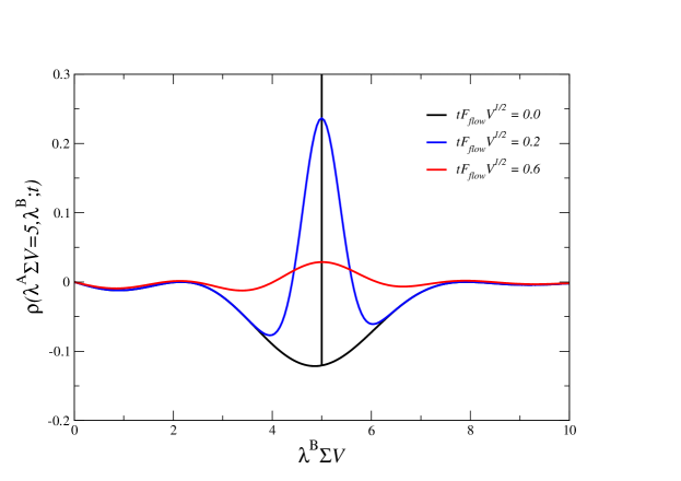
Figure 3: The two-point correlation function between the spectrum at zero flow time and at non-zero flow time. The zero flow time eigenvalue is fixed at $\lambda^{A}\Sigma V=5$. This automatically implies that at zero flow time there is an eigenvalue at $\lambda^{B}\Sigma V=5$ and hence a $\delta$-function in the two-point correlation function, as indicated by the vertical line. For small flow time the primary effect of the flow is to smoothen this $\delta$-function. The graphs are for $\sqrt{V}F_{\rm flow}t=0.0$, $\sqrt{V}F_{\rm flow}t=0.2$ and $\sqrt{V}F_{\rm flow}t=0.6$ and $\nu=0$.

The $t\to 0$ limit is also analytically accesible and agrees with the $t=0$ two point function TVspect

$$\rho(\lambda^{A},\lambda^{B};t=0) = \delta(\hat{\lambda}^{A}-\hat{\lambda}^{B})\frac{\hat{\lambda}^{A}}{2}\left[J_{\nu}^{2}(\hat{\lambda}^{A})-J_{\nu+1}(\hat{\lambda}^{A})J_{\nu-1}(\hat{\lambda}^{A})\right]$$

$$-\frac{\hat{\lambda}^{A}\hat{\lambda}^{B}}{((\hat{\lambda}^{A})^{2}-(\hat{\lambda}^{B})^{2})^{2}}\left[\hat{\lambda}^{A}J_{\nu+1}(\hat{\lambda}^{A})J_{\nu}(\hat{\lambda}^{B})-\hat{\lambda}^{B}J_{\nu+1}(\hat{\lambda}^{B})J_{\nu}(\hat{\lambda}^{A})\right]^{2}\,.$$

Note that the $\delta$-function in the first line is multiplied by the quenched spectral density (4.1). As $t$ grows from zero this $\delta$-function is smeared as discussed in the previous section. For $t$ close to zero, Eq. (4.2.1) can also be evaluated analytically. The Bessel function $I_{\nu}$ can be approximated by its asymptotic form while the exponents in the integrals over $\alpha$ can be put equal to 1. This results in

$$\rho(\lambda^{A},\lambda^{B};t)=\frac{\rho(\lambda_{A})}{\sqrt{8\pi VF_{\rm flow}^{2}t^{2}}}\exp\left(-\frac{(\hat{\lambda}^{A}-\hat{\lambda}^{B})^{2}}{8VF_{\rm flow}^{2}t^{2}}\right)+Y_{2}(\lambda^{A},\lambda^{B}),$$ (63)

where $Y_{2}(\lambda^{A},\lambda^{B})$ represents the second term in Eq. (4.2.1). For small $t$, the width of the Gaussian distribution is given by

$$\sigma=2F_{\rm flow}t\sqrt{V}.$$ (64)

The smearing of the $\delta$-function can also be seen in Fig. 3 where we plot the evolution of the spectral two-point correlation function for fixed $\hat{\lambda}^{A}$ as a function of $\hat{\lambda}^{B}$ and $F_{\rm flow}\sqrt{V}t=0,$ 0.2 and $0.6$. The smearing of the $\delta$-function shows that the microscopic spectrum of $D(B_{\mu})$ decorrelates from that of $D(A_{\mu})$ on the timescale set by $t\thicksim 1/(F_{\rm flow}\sqrt{V})$.

The analytical form of the two point function offers an efficient tool to extract the value of $F_{\rm flow}$ from a given flow on the lattice: The width of the peak depends linearly on $F_{\rm flow}$, and a fit of the analytical curve to lattice data offers a way to measure $F_{\rm flow}$. (A similar approach has successfully been used to extract the value of the pion decay constant, see DHSS ; DHSST ; Damgaard:2006pu ; Lehner:2009pz ; AD .) Different flow equations which preserve the same symmetries will lead to different values of $F_{\rm flow}$, and one may use the spectral two-point function to find the flow with the smallest value of $F_{\rm flow}$ and hence the flow which best preserves the dynamical properties of the microscopic eigenvalues.

5 Conclusions and Discussion

We have constructed the low energy theory for the gradient flow of the Dirac eigenvalues to leading order in the flow time. This theory is an extended version of partially quenched chiral perturbation theory, where to leading order an additional term proportional to $t^{2}$ competes with the mass term. The new term of order $t^{2}$ comes with a new low energy constant, $F_{\rm flow}^{2}$, the value of which depends on the detailed form of the flow equations.

Using this chiral Lagrangian we have computed the spectral resolvent of the Dirac operator for gauge fields at non-zero flow time. For valence quark mass equal to the physical quark mass, it coincides with the chiral condensate due to the flow of the gauge fields but with no flow of the fermion fields. The eigenvalue density of the Dirac operator at non-zero flow time is given by the spectral resolvent evaluated at a purely imaginary valence quark mass. We have computed this eigenvalue density explicitly in the $\epsilon$-regime.

These results give insights in the changes with flow time of the dynamical properties of the simulation, carried out at zero flow time. Since the flow equation for the gauge field has no direct connection to the fermionic part of the action it is natural to expect that the characteristic features of dynamical simulations, such as eigenvalue repulsion from the quark mass, will be absent at large flow time. Indeed the results derived here for the mass dependence of the spectral resolvent and the unquenched eigenvalue density are both driven by the flow to their quenched form. The quenched results in the $\epsilon$-domain are obtained when the flow time satisfies $F^{2}_{\rm flow}t^{2}V\gg 1$. The new low energy constant $F_{\rm flow}$ in this sense measures the degree to which the flow preserves the dynamical properties of the microscopic eigenvalues at small energies. Different flow equations will result in different values of $F_{\rm flow}$ which raises the question whether there is a systematic way to optimize the flow equations such that the value of $F_{\rm flow}$ is minimized and hence the dynamical properties of the initial configurations are better preserved. The spectral two point function, also determined here, offers an ideal way measure the value of $F_{\rm flow}$ in simulations. For small flow time this constant follows immediately from the width of the peak in the two-point function.

Within the $\epsilon$-counting scheme for the spectral resolvent we require that $F_{\rm flow}^{2}t^{2}V\thicksim 1$ and only a single new term appears in the chiral Lagrangian at leading order. This allowed us to follow the evolution of the microscopic spectral observables with flow time. For a larger scaling of the flow time we would not have been able to resolve this dependence. Suppose we had allowed $t$ to be of order $1/L$, then the microscopic eigenvalues would have decorrelated immediately from the fermion determinant.

A flow time of order $1/L$ is the natural scale when considering the spectral correlation functions in the $p$-regime of chiral perturbation theory, since the $t^{2}$ term in the chiral Lagrangian competes with the mass term for $t\thicksim 1/L$ (we have $m_{\pi}^{2}F_{\pi}^{2}\thicksim t^{2}F_{\rm flow}^{2}$ if $m_{\pi}\thicksim t\thicksim 1/L$). Using this $p$-regime counting it would be most interesting to work out the corrections to the Smilga-Stern relation SmilgaStern due to the flow.

All results presented here lend themselves to a direct test in Lattice QCD. For an existing dynamical simulation one needs to compute the flow of the gauge fields and determine the low lying eigenvalues of the Dirac operator evaluated in these backgrounds. Such a computation will give direct insights in the conservation of the dynamical properties of the spectral observables during the flow. Moreover it will determine if chiral perturbation theory captures this aspect of gradient flow.

Finally it would be interesting to generalize the results obtained here for the $\epsilon$-regime of chiral perturbation theory to an arbitrary number of flavors. It would also be useful to obtain explicit expressions for individual eigenvalue distributions. Starting from AD ; AI such a computation appears to be within reach.

Acknowledgments: We would like to thank Poul Henrik Damgaard, Joyce C. Myers, Peter Pedersen as well as participants of the workshop ’Facing Strong Dynamics’ for discussions. KS would like to thank the CERN theory division for hospitality during the completion of this project and the participants of the workshop ’Conceptual advances in Lattice gauge theory’ for discussions. This work was supported by the Lørup foundation (ASC), U.S. DOE Grant No. DE-FG-88ER40388 (JV) and the Sapere Aude program of The Danish Council for Independent Research (KS).

Appendix A $\langle{\cal S}^{0}_{t}\rangle$ for $N_{f}=1$ by explicit parmetrization

In this appendix we outline the derivation of $\langle{\cal S}^{0}_{t}\rangle$ for $N_{f}=1$ as obtained from an explicit parameterization of the graded partition function at nonzero flow time

$$Z_{2|1}(m,m_{v},m_{v}^{\prime};t)=\int_{Gl(2|1)}{\cal D}U\,e^{\frac{1}{2}{\rm Str}\left[{\cal M}(U+U^{-1})\right]+t^{2}F_{\rm flow}^{2}V{\rm Str}\left[{\cal T}U^{-1}{\cal T}U\right]}\,.$$ (65)

Here ${\cal M}={\rm Diag}(m,m_{v},m_{v}^{\prime})$ and ${\cal T}={\rm Diag}(0,1,1)$. Note that in this Appendix we have absorbed a factor of $\Sigma V$ into $m$, $m_{v}$ and $m_{v}^{\prime}$ in order to lighten the notation. To parameterize $U$ we choose

$$U = \left(\begin{array}[]{ccc}e^{it+iu}\cos\theta&ie^{it+i\phi}\sin\theta&0\\ ie^{it-i\phi}\sin\theta&e^{it-iu}\cos\theta&0\\ 0&0&e^{s}\end{array}\right)\exp\left(\begin{array}[]{ccc}0&0&\alpha_{1}\\ 0&0&\alpha_{2}\\ \beta_{1}&\beta_{2}&0\end{array}\right)\,,$$ (72)

where $\theta,t,u\in[-\pi,\pi]$, $\phi\in[0,\pi]$ and $s\in[-\infty,\infty]$. The corresponding Jacobian and Berezinian are DOTV

$$J=4e^{4it}\cos\theta\sin\theta\,,\qquad B=1+\frac{1}{3}(\alpha_{1}\beta_{1}+\alpha_{2}\beta_{2})\,.$$ (73)

The Grassmann integrals can be carried out analytically and result in the partition function

$$Z_{2|1}(m,m_{v},m_{v}^{\prime};t)$$

$$= \int_{-\infty}^{\infty}{\rm d}s\int_{0}^{\pi}{\rm d}\phi\int_{-\pi}^{\pi}{\rm d}t\int_{-\pi}^{\pi}{\rm d}u\int_{-\pi}^{\pi}{\rm d}\theta\ |J|\ (P_{4}^{t}-P_{11}^{t}P_{22}^{t}+P_{12}^{t}P_{21}^{t}-\frac{1}{3}P_{11}^{t}-\frac{1}{3}P_{22}^{t})\ e^{S^{t}},$$

where

$$S^{t}=m\cos(t+u)\cos\theta+m_{v}\cos(t-u)\cos\theta-m_{v}^{\prime}\cosh s-t^{2}F_{\rm flow}^{2}V\sin^{2}\theta\,,$$ (75)

and

$$P_{11}^{t} = \,\frac{m}{2}\cos(t+u)\cos\theta+\frac{m_{v}^{\prime}}{2}\cosh s+t^{2}F_{\rm flow}^{2}V\cos^{2}\theta\,,$$

$$P_{22}^{t} = \,\frac{m_{v}}{2}\cos(t-u)\cos\theta+\frac{m_{v}^{\prime}}{2}\cosh s\,,$$

$$P_{12}^{t} = \,-\frac{im}{4}e^{-it-i\phi}\sin\theta+\frac{im_{v}}{4}e^{it-i\phi}\sin\theta-t^{2}F_{\rm flow}^{2}V\tfrac{i}{2}\cos\theta\sin\theta e^{iu-i\phi}\,,$$ (76)

$$P_{21}^{t} = \,\frac{im}{4}e^{it+i\phi}\sin\theta-\frac{im_{v}}{4}e^{-it+i\phi}\sin\theta+t^{2}F_{\rm flow}^{2}V\tfrac{i}{2}\cos\theta\sin\theta e^{-iu+i\phi}\,,$$

$$P_{4}^{t} = \,\frac{m}{24}\cos(t+u)\cos\theta+\frac{m_{v}}{24}\cos(t-u)\cos\theta+\frac{m_{v}^{\prime}}{12}\cosh s+t^{2}F_{\rm flow}^{2}V\frac{1+2\sin^{2}\theta}{12}\,.$$

The $\phi$ dependence of the integrand cancels, and thus the $\phi$-integration trivially yields an overall factor of $\pi$. It is furthermore possible to express the $s$-integration in terms of modified Bessel functions of the second kind, using

$$\int_{-\infty}^{\infty}{\rm d}s\,e^{-m\cosh s} = 2K_{0}(m)\,,$$

$$\int_{-\infty}^{\infty}{\rm d}s\,e^{-m\cosh s}\cosh s = 2K_{1}(m)\,,$$ (77)

$$\int_{-\infty}^{\infty}{\rm d}s\,e^{-m\cosh s}\cosh^{2}s = K_{0}(m)+K_{2}(m)\,.$$

This allows for writing the generation functional as

$$Z_{2|1}(m,m_{v},m_{v}^{\prime};t)=\pi\int_{-\pi}^{\pi}{\rm d}t\int_{-\pi}^{\pi}{\rm d}u\int_{-\pi}^{\pi}{\rm d}\theta\,|J|\,(P_{0}^{t}+P_{1}^{t}+P_{2}^{t})\,e^{S_{\rm int}^{t}}\,,$$ (78)

where

$$S_{\rm int}^{t}=m\cos(t+u)\cos\theta+m_{v}\cos(t-u)\cos\theta-t^{2}F_{\rm flow}^{2}V\sin^{2}\theta\,,$$ (79)

and

$$P_{0}^{t} = \,2K_{0}(m_{v}^{\prime})\Bigg{[}P_{12}^{t}P_{21}^{t}$$

$$+\bigg{\{}\frac{m}{24}\cos(t+u)\cos\theta+\frac{m_{v}}{24}\cos(t-u)\cos\theta-t^{2}F_{\rm flow}^{2}V\frac{1+2\sin^{2}\theta}{12}\bigg{\}}_{4}$$

$$-\bigg{\{}\Big{(}\frac{m}{2}\cos(t+u)\cos\theta+t^{2}F_{\rm flow}^{2}V\cos^{2}\theta\Big{)}\Big{(}\frac{m_{v}}{2}\cos(t-u)\cos\theta\Big{)}\bigg{\}}_{\begin{subarray}{c}11\\ 22\end{subarray}}$$

$$-\frac{1}{3}\bigg{\{}\frac{m}{2}\cos(t+u)\cos\theta+t^{2}F_{\rm flow}^{2}V\cos^{2}\theta\bigg{\}}_{11}-\frac{1}{3}\bigg{\{}\frac{m_{v}}{2}\cos(t-u)\cos\theta\bigg{\}}_{22}\Bigg{]}\,,$$

$$P_{1}^{t} = \,-\frac{m_{v}^{\prime}}{2}K_{1}(m_{v}^{\prime})\left[1+m_{v}\cos(t-u)\cos\theta-m\cos(t+u)\cos\theta-2t^{2}F_{\rm flow}^{2}V\cos^{2}\theta\right]\,,$$

$$P_{2}^{t} = \,-\frac{m_{v}^{\prime}}{4}[K_{0}(m_{v}^{\prime})+K_{2}(m_{v}^{\prime})]\,.$$

The subscripts on the curly brackets are only reminders of where the term originates from in (76).

The parameterization allows for a semi-analytical calculation of the spectral resolvent as a function of $m$ and at non-zero flow time from

$$\langle{\cal S}^{0}_{t}\rangle_{m,m_{v};t}=\frac{1}{Z_{2|1}(m,m_{v},m_{v};t)}\,\partial_{m_{v}}Z_{2|1}(m,m_{v},m_{v}^{\prime};t)\bigg{|}_{m_{v}=m_{v}^{\prime}}\,.$$ (81)

Note that $Z_{2|1}(m,m_{v},m_{v};t)=Z_{1}(m)$.

References

- (1) M. Lüscher, Commun. Math. Phys. 293, 899 (2010) [arXiv:0907.5491 [hep-lat]].
- (2) M. Lüscher, JHEP 1008, 071 (2010) [arXiv:1006.4518 [hep-lat]].
- (3) M. Lüscher and P. Weisz, JHEP 1102, 051 (2011) [arXiv:1101.0963 [hep-th]].
- (4) M. Lüscher, JHEP 1304, 123 (2013) [arXiv:1302.5246 [hep-lat]].
- (5) H. Makino and H. Suzuki, PTEP 2014, no. 6, 063B02 (2014) [arXiv:1403.4772 [hep-lat]].
- (6) L. Del Debbio, A. Patella and A. Rago, JHEP 1311, 212 (2013) [arXiv:1306.1173 [hep-th]].
- (7) Z. Fodor, K. Holland, J. Kuti, S. Mondal, D. Nogradi and C. H. Wong, arXiv:1406.0827 [hep-lat].
- (8) A. Ramos and S. Sint, talk at ’Conceptual advances in lattice gauge theory (LGT14)’, CERN July 2014.
- (9) P. H. Damgaard and S. M. Nishigaki, Nucl. Phys. B 518, 495 (1998) [hep-th/9711023].
- (10) T. Wilke, T. Guhr and T. Wettig, Phys. Rev. D 57, 6486 (1998) [hep-th/9711057].
- (11) P. H. Damgaard, J. C. Osborn, D. Toublan and J. J. M. Verbaarschot, Nucl. Phys. B 547, 305 (1999) [hep-th/9811212].
- (12) M. E. Berbenni-Bitsch, S. Meyer and T. Wettig, Phys. Rev. D 58, 071502 (1998) [hep-lat/9804030].
- (13) P. H. Damgaard, U. M. Heller, R. Niclasen and K. Rummukainen, Phys. Lett. B 495, 263 (2000) [hep-lat/0007041].
- (14) H. Fukaya et al. [JLQCD and TWQCD Collaborations], Phys. Rev. D 83, 074501 (2011) [arXiv:1012.4052 [hep-lat]].
- (15) O. Bar and M. Golterman, Phys. Rev. D 89, 034505 (2014) [arXiv:1312.4999 [hep-lat]].
- (16) A. Shindler, Nucl. Phys. B 881, 71 (2014) [arXiv:1312.4908 [hep-lat]].
- (17) J. Gasser and H. Leutwyler, Annals Phys. 158, 142 (1984).
- (18) J. Gasser and H. Leutwyler, Phys. Lett. B 188, 477 (1987).
- (19) H. Leutwyler and A. V. Smilga, Phys. Rev. D 46, 5607 (1992).
- (20) P. H. Damgaard, U. M. Heller, K. Splittorff, B. Svetitsky and D. Toublan, Phys. Rev. D 73, 105016 (2006) [hep-th/0604054].
- (21) J. J. M. Verbaarschot and I. Zahed, Phys. Rev. Lett. 70, 3852 (1993) [hep-th/9303012].
- (22) P. H. Damgaard, U. M. Heller, K. Splittorff and B. Svetitsky, Phys. Rev. D 72, 091501 (2005) [hep-lat/0508029].
- (23) P. H. Damgaard, U. M. Heller, K. Splittorff, B. Svetitsky and D. Toublan, Phys. Rev. D 73, 074023 (2006) [hep-lat/0602030].
- (24) K. Splittorff and J. J. M. Verbaarschot, Phys. Rev. Lett. 90, 041601 (2003) [cond-mat/0209594].
- (25) D. Sherrington and S. Kirkpatrick, Phys. Rev. Lett. 35, 1792 (1975).
- (26) P. H. Damgaard and K. Splittorff, Phys. Rev. D 62, 054509 (2000) [hep-lat/0003017].
- (27) E. Kanzieper, Nucl. Phys. B 596, 548 (2001) [cond-mat/9908130].
- (28) K. Splittorff and J. J. M. Verbaarschot, Nucl. Phys. B 683, 467 (2004) [hep-th/0310271].
- (29) D. Toublan and J. J. M. Verbaarschot, Nucl. Phys. B 603, 343 (2001) [hep-th/0012144].
- (30) C. Lehner and T. Wettig, JHEP 0911, 005 (2009) [arXiv:0909.1489 [hep-lat]].
- (31) G. Akemann and P. H. Damgaard, JHEP 0803, 073 (2008) [arXiv:0803.1171 [hep-th]].
- (32) A. V. Smilga and J. Stern, Phys. Lett. B 318, 531 (1993).
- (33) G. Akemann and A. C. Ipsen, J. Phys. A 45, 115205 (2012) [arXiv:1110.6774 [hep-lat]].