Truthful Prioritization Schemes for Spectrum Sharing

Abstract

We design a protocol for dynamic prioritization of data on shared routers such as untethered 3G/4G devices. The mechanism prioritizes bandwidth in favor of users with the highest value, and is incentive compatible, so that users can simply report their true values for network access. A revenue pooling mechanism also aligns incentives for sellers, so that they will choose to use prioritization methods that retain the incentive properties on the buy-side. In this way, the design allows for an open architecture. In addition to revenue pooling, the technical contribution is to identify a class of stochastic demand models and a prioritization scheme that provides allocation monotonicity. Simulation results confirm efficiency gains from dynamic prioritization relative to prior methods, as well as the effectiveness of revenue pooling.

1 Introduction

Many mobile broadband data users overpay for data plans, buying a data plan with sufficient monthly quota for their maximum needs even though the average consumption is only about 15% of the monthly quota [1]. Analysis of cell phone data has also shown quota dynamics [2] in users, i.e., sensitivity to quota balance and time to the end of the quota period. One way to address these inefficiencies is to allow surplus bandwidth to be shared. In this paper we propose an auction-based protocol for such bandwidth-sharing. Sellers have wireless broadband (3G/4G) devices with a WiFi like WLAN radio, and can share network access through tethering apps that allow them to act as routers. Buyers have WiFi devices and pay sellers to relay their data.

Rather than finding optimal static allocations to users, our focus is on dynamic prioritization of access to bandwidth. Dynamic prioritization is more efficient because it can handle temporal heterogeneity in user demand. We design an auction protocol to prioritize network access in favor of those with highest value. In ensuring simplicity for users, we seek an incentive compatible design, so that truthful reporting of value and straightforward use of the shared bandwidth (no delaying of traffic, no padding of traffic) is optimal for a user. Incentive compatibility is also useful in avoiding “churn” and system overhead that can occur if users can benefit by adapting reported values given reports of others. Similar arguments have been made in the context of sponsored search markets [7].

Our positive results are stated for users with linear (per-byte) valuation functions. Give this, incentive compatibility requires that the cumulative quantity of network resources consumed by a user is non-decreasing in bid value, a property referred to as monotonicity. Our main technical contribution is to establish conditions on user demand models for which a strict priority-queue approach to resource access control satisfies monotonicity. An important property satisfied by the demand models is that a user’s cumulative consumption of network bandwidth over a user session weakly increases as a function of her total consumption up to any intermediate time. An additional technical challenge that we address is to ensure that users cannot benefit through delayed use of allocated network resources, or by introducing fake traffic to increase demand.

Payments are computed by adopting an approach due to Babaioff, Kleinberg, and Slivkins [4] (bks). This involves adding an additional, random perturbation to bids. In a typical auction setting, the auctioneer knows how an allocation of resources would have changed given different bids. This counterfactual information is essential to standard payment schemes but unavailable here. It would require knowledge of how much bandwidth a user would consume under a different priority, but this requires knowledge that the network infrastructure does not have about a user’s demand model. The only information available for the purpose of determining payments is the actual realization of consumption based on the actual assignment of priority. The introduction of random perturbation by the bks scheme avoids the need for this counterfactual information.

We also extend our design so that it embraces open network architectures. In particular, we are robust to router devices that can install alternative routing software, for example to change prioritization schemes, or otherwise tamper with methods to compute payments. Thus, we seek to align incentives on the sell side as well as the buy side of the market. Our solution adopts lightweight cryptography and revenue pooling across sellers, and has the effect of aligning the interests of sellers with adopting routing policies that maximize total buyer value. This is sufficient for monotonicity of user allocations, which is in turn sufficient for buyer truthfulness. Revenue pooling makes the market design appear simultaneously as a first-price market for sellers and a second-price market for buyers. For sellers, this means they prefer to maximize the (bid) value of the allocation. For buyers, this retains the second-price-like bks scheme, and thus incentive compatibility.

A simulation study confirms that the mechanism achieves arbitrarily close approximations to full allocative efficiency for simple demand models (allocating the shared resource to those who value it the most), shows that reserve prices can increase efficiency of non-prioritized routing methods, demonstrates a scenario where sellers have practical efficiency-improving deviations, and examines the distributional effects of revenue pooling. We have also prototyped our scheme using the traffic control module in the Linux kernel.

1.1 Related work

Sen et al. [18] provide an exhaustive survey of the large literature on smart data pricing. We focus on describing work related to the specific techniques that we use.

Babaioff et al. [5] and Devanur et al. [6] show that the unavailability of counterfactuals impedes the design of truthful mechanisms in the context of multi-armed bandit problems. We employ the bks scheme in a new application domain. The effect is that the payment scheme that we adopt accounts for varying user demand, providing an unbiased estimate of the cost imposed on other buyers by the prioritization associated with a buyer’s device. In contrast, an earlier scheme due to Varian and Mackie-Mason (VMM) [22] adopts a myopic, per-packet viewpoint on the cost imposed on other users and is not incentive compatible when buyers have adaptive demand patterns.

Other approaches from dynamic mechanism design are unsuitable, either because they rely on counterfactual information [10] or rely on a probabilistic demand model [16]. VMM’s work inspired other approaches, such as the progressive second-price auction [11], and some follow-on work [12]. As with VMM, they also do not achieve incentive alignment in dynamic settings. They also assume the existence of a trusted router.

Godfrey et al. [8] study incentive compatibility of congestion control mechanisms in networks. Our technical analysis of the separation between bidders is similar to the separation between flows in this earlier model, but the domain of study and main results are otherwise incomparable. We consider user bidding and payments, whereas they analyze the effect of manipulations in forwarding strategies on network-wide congestion.

In a different domain, Shneidman and Parkes [21] study the problem of faithful network protocols for BGP routing, where the algorithms adopted by network users must themselves form part of an equilibrium. In this sense, our revenue pooling scheme attains faithfulness with respect seller routing algorithms.

Also related is a large literature on the use of cryptographic solutions to provide trustworthy auctions; e.g. [15]. However, these solutions incur too much overhead in the context of dynamic bandwidth prioritization. Porter and Shoham [17] provide an analysis of how the presence of cheating provides a second-price auction with first-price semantics. Our revenue pooling scheme, used for aligning trust does the opposite: we give a second-price auction first-price semantics from the perspective of the auctioneer (or seller, in our model), thereby mitigating incentives for manipulation; the scheme borrows ideas from a random-sampling approach used in a very different domain, that of the design of revenue-optimal digital good auctions [9].

2 Model

In this section we describe our model, also shown in Fig. 1.

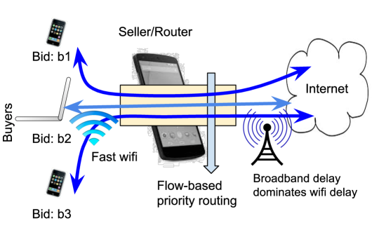
Figure 1: Illustration of our model.

Time and value: Time is modeled in discrete epochs. Each buyer (agent) $i$ has an allocation period $[\alpha_{i},\beta_{i}]$, with $\alpha_{i}\geq 0$ and $\beta_{i}\geq\alpha_{i}$. This is the period of time over which the buyer associates value with receiving bandwidth. Each buyer has constant value $v_{i}\geq 0$ per byte (a linear valuation), and bids once before sending data.

Routing: We adopt a flow model of traffic, with a single flow modeling both upstream and downstream traffic for each buyer. The router’s link to the Internet is assumed to have fixed capacity $c>0$. Each buyer has bid $b_{i}\geq 0$, and receives a priority based on this reported value.

We consider three schemes for network prioritization:

1. First-in First-out (fifo) routes data in a first-in, first-out order as it arrives at the router. Since we do not model the queue of a router directly, we model fifo as a within-epoch allocation proportional to within-epoch demand.

2. Fair queueing (fq) allocates bandwidth to all buyers evenly, dividing any unused capacity recursively: in each period, each of the $n$ buyers is guaranteed to be able to consume $c/n$. Any unused capacity is divided evenly among buyers with further demand, and this repeats until everyone is satisfied or capacity is exhausted.

3. Strict Priority Queueing (spq) first allocates capacity to the buyer with the highest bid in each epoch, up to $c$ or the demand of the buyer. Then, capacity is allocated to the buyer with the second highest bid, and so forth, as long as capacity is available. Ties are broken at random.

Let $c_{i,t}$ denote the network capacity available to buyer $i$ in epoch $t$ (this depends on her bid, as well as the bid and network usage of others.)

Transport: We assume that the local network between router and buyers is much faster than the router’s link to the Internet and neglect delays there.

Demand: Let $x_{i,t}$ (bytes) denote the cumulative amount of traffic (upload or download) associated with buyer $i$ up to and including time $t$. This may be smaller than the total capacity available to buyer $i$ up to and including time $t$ because it depends on the buyer’s demand.

Let $D_{i}(t,x)$ (bytes) denote the demand of buyer $i$ during epoch $t$, where $x$ is the cumulative amount of traffic (upload or download) used so far; i.e., $x=x_{i,t-1}$. Equivalently, this represents the maximum amount of network capacity that buyer $i$ wants to consume during the epoch. $D_{i}(t,x)$ is a random variable, and we adopt $d_{i}(t,x)$ to denote a specific realization. We consider demand models $D_{i}$ that satisfy the following condition:

Definition 1.

A demand model $D_{i}(t,x)$ is natural if all realizations $d_{i}(t,x)$ satisfy for all $t$, for all $x\geq x^{\prime}$ and all $c\geq 0$:

$$x+\min(c,d_{i}(t,x))\geq x^{\prime}+\min(c,d_{i}(t,x^{\prime})).$$

A demand model is natural when getting more capacity earlier might increase demand in the future, and should not decrease future demand below the total amount given lower capacity. In presenting some examples of demand models that are natural in this sense, we focus on deterministic examples. Randomized models can be created through random perturbations to the parameters of the example, and also through randomization over the different kinds of models.

Constant demand: A buyer $i$ who simply wants to send at some constant rate: $d_{i}(t,x)=k$.

Time-varying demand: A buyer $i$ with an arbitrary time-dependent generation process $g(t)$ that generates data that must be sent immediately to be useful: $d_{i}(t,x)=g(t)$.

Buffered demand: A buyer $i$ with an arbitrary time-dependent generation process $g(t)$ that generates data, and wants to send as much of that as possible, buffering demand until it is allocated: $d_{i}(t,x)=\sum_{p\leq t}g(p)-x$.

Impatient buyer: A buyer $i$ who sends until time $p$, and then goes away if some minimum amount of service $m$ has not been met:

$$d_{i}(t,x)=\begin{cases}k\text{ if }t\leq p\\ k\text{ if }t>p\text{ and }x>m\\ 0\text{ else }\end{cases}$$

This can be generalized to multiple thresholds, reduction to a lower, but non-zero rate, etc.

Increasing demand (in rate) A buyer that has $d_{i}(t,x)=g(x/t)$, with $g$ weakly increasing.

Increasing demand (in total) A buyer that has $d_{i}(t,x)=g(x)$, with $g$ weakly increasing.

This impatient buyer model illustrates that the requirement of ”natural” demand functions allow those users to be modeled whose future value for network access falls if they don’t receive enough bandwidth.

These demand models capture many realistic types of demand, but some demand functions do not fit our model. In particular, we do not allow demand to depend on recent usage, precluding models like “if I have not been able to use the network in the last 30 seconds, give up”.

3 Prioritization and Payments

Having introduced the basic elements of our model, we now describe some variations on payment schemes.

3.1 Fixed price

A baseline comparison is provided by a fixed price payment scheme. This can be used together with the fifo and fq routing policies, where only the users who bid above the fixed price are considered by the prioritization schemes.

3.2 VMM mechanism

The vmm mechanism provides a second comparison point. This mechanism uses the spq routing policy. For payments, the original paper by Varian and Mackie-Mason used a per-packet model, and charged the owner of each forwarded packet the immediate externality imposed by the packet. This is the value of the highest value packet that was dropped while the forwarded packet was in the router’s queue.

Since we do not model the router queue directly, we adapt the idea behind the payment mechanism to our flow-based model by charging the immediate externality imposed by a buyer’s flow in each period, computed using the standard Vickrey-Clarke-Groves (vcg) mechanism, charging $V_{-i}-V^{*}_{-i}$ for each buyer $i$ in each period, where $V_{-i}$ is the total (reported) value to all the other buyers in the (counterfactual) optimal allocation when $i$ is removed, and $V^{*}_{-i}$ is the total (reported) value to all the other buyers in the real optimal allocation with $i$ included.

vmm is a natural mechanism, and has inspired a lot of work on bandwidth pricing. However, the vmm approach is not incentive compatible in a setting with variable demand. Consider the following:

Example 1. Suppose that the router link capacity is 1 packet per second, and there is one buyer with value $3 per packet who wants to send one packet every second and a second buyer with value $2 per packet who wants to send a single packet, and keeps trying until she succeeds. Truthful bidding by buyer 1 will result in the second buyer’s packet being dropped every period, and a charge of $2 for each packet, representing the per-epoch externality on buyer 2. On the other hand, a bid of less than $2 would “flush” the packet of buyer 2 and then allow buyer 1 to send for the remaining epochs with payment $0. The tradeoff is to reduce the amount of data forwarded by 1 packet in return for a significant reduction in total payment.

3.3 The BKS Mechanism

In the example above, vmm over-estimates the externality because it does not have access to the information that buyer 2 only has a single packet to send. This information is not available, since we assume that demand models are not described by users or known by the prioritization scheme. In fact, even the user themselves may not know their future demand before it is realized.

In this domain, the bks mechanism adopts the spq routing policy. Payments are determined following a self-sampling approach, where a randomized perturbation to bids obviates the need for counterfactual information. The idea is to obtain an estimate of the network resources that a user would have consumed at some lower bid as a side-effect of the randomization.

We adapt the scheme to also allow the seller to employ a reserve price $r\geq 0$, which is the minimal per-byte price a seller will accept. The scheme is parameterized by $\mu\in(0,1)$, which governs the probability of introducing a random perturbation into bids.

The scheme is most easily explained in terms of an allocation rule $\mathcal{A}$. For us, this encapsulates the combined effect of realized demand (including possible strategic effects by users delaying demand or creating fake demand), the routing policy, the total capacity constraint on the router, and user bids. Taken together, these elements define the total amount of traffic consumed by each user (equivalently, the realized allocation).

The allocation $\mathcal{A}(\tilde{b},d)$ generated by the rule is ex ante uncertain—it depends on realized demand $d=(d_{1},\ldots,d_{n})$, where $d_{i}$ denotes the realized demand by $i$ in each epoch, and is applied to randomly perturbed bids $\tilde{b}$. The bks payment scheme works as follows:

Definition 2 (bks).

Given an allocation rule $\mathcal{A}$ and a parameter $\mu\in(0,1)$, the bks procedure in our setting is:

1. Upon arrival, each bidder $i$ submits a bid $b_{i}\geq r$.

2. The mechanism computes transformed bids $\tilde{b}_{i}$ $\forall$ $i$:

   1. With probability $1-\mu$, $\tilde{b}_{i}=b_{i}$

   2. Else, compute a reduced bid: pick $\gamma\in[0,1]$ uniformly at random, and set $\tilde{b}_{i}=r+(b_{i}-r)\cdot\gamma^{1/(1-\mu)}$

3. For all epochs, the router uses the allocation rule $\mathcal{A}(d,\tilde{b})$ applied to the transformed bids $\tilde{b}$ of the active users and given realized demand $d=(d_{1},\ldots,d_{n})$.

4. Given the amount of network data, $x_{i}\geq 0$, associated with each user $i$, (as realized by the allocation rule $\mathcal{A}$ applied to transformed bids), collect payment from user $i$ as:

   1. Collect $b_{i}x_{i}$.

   2. If $\tilde{b}_{i}<b_{i}$, give a rebate $R_{i}=\frac{1}{\mu}(x_{i}(b_{i}-r))$. Otherwise, $R_{i}=0$.

Bids are perturbed, used for prioritized routing, the total number of bytes associated with a user is observed, and payments are made through a randomized adjustment via the rebate in step 4. Each user’s rebate can be determined at the end of her allocation period, allowing the user’s payment to be computed while other users are still active.

Definition 3.

A mechanism is truthful-in-expectation if a risk-neutral buyer maximizes expected utility by bidding truthfully, whatever the bids of others, where the expectation is taken with respect to random coin flips of the mechanism.

An essential property for truthfulness is the ex post monotonicity of the allocation rule.

Let $\mathcal{A}_{i}(b^{\prime},d)$ denote the allocation to buyer $i$ given some bid vector $b^{\prime}$ and demand vector $d$. (We write $b^{\prime}$ to denote a generic bid vector and avoid confusion with the $b$ submitted as input to bks.) An allocation rule is ex post monotone if $\mathcal{A}_{i}(b^{\prime\prime},d)\geq\mathcal{A}_{i}(b^{\prime},d)$, for all bid vectors $b^{\prime}$, all demand vectors $d$, and all $b^{\prime\prime}=(b^{\prime}_{1},\ldots,b_{i}^{\prime\prime},\ldots,b^{\prime}_{n})$ such that $b^{\prime\prime}_{i}>b^{\prime}_{i}$. This is ex post in the sense that whatever the bids and whatever the demand, a buyer’s total traffic consumption weakly increases with her bid. We use the following result:

Theorem 3.1.

Applying the bks procedure with probability of perturbation $\mu$ to an allocation rule that is ex post monotone results in a truthful-in-expectation mechanism.

The proof in [4] shows that the scheme obtains an unbiased sample of an integral that defines the payment rule in the canonical approach of incentive-compatible mechanism design [13]. The allocation is the same as in the original allocation rule with probability at least $1-n\mu$, where $n$ is the number of buyers.

Example 2. Let’s revisit the earlier example of manipulation in the vmm scheme. Under bks, when the first buyer’s bid is not resampled, she pays $3 per packet, and has some total allocation $k$. When her bid is resampled, the first buyer will have allocation $k$ or $k-1$, depending on whether the resampled bid was below $2. This will result in a large rebate, and in expectation, the first buyer’s total payment will be essentially $2, with the exact value depending on $\mu$.

4 Buyer incentives

To establish truthfulness of the bks mechanism in our setting we need to show that spq combined with natural demand models implies that the allocation rule is ex post monotone. In our setting, the allocation rule is the process that determines the total network traffic used by each buyer over her allocation period.

We first show that spq provides an isolation property on buyers, and then analyze the monotonicity of our allocation rule.

Lemma 4.1 (isolation).

For any $t$, capacity $c_{i,t}$ under spq is independent of how capacity is used by buyer $i$ in time $<t$, and weakly increases with bid $b_{i}$.

Proof.

Consider $n$ buyers, and order them by bids $b_{1}\geq b_{2}\geq\ldots\geq b_{n}$ with ties broken at random. Let’s first consider the claim that capacity $c_{i,t}$ in epoch $t$ is independent of how the capacity is used by buyer $i$ in earlier epochs. Proceed by strong induction. For buyer 1, then this is immediate since the buyer always gets to use full the capacity of the channel. For buyer $i>1$, given the induction hypothesis for buyers $<i$, buyer $i$ cannot affect demand or allocation to higher priority buyers and is not affected by the use of the capacity by lower priority buyers. The result is that buyer $i$ gets all capacity that is unused by the higher priority buyers. The capacity $c_{i,t}$ is weakly increasing with bid value because of spq routing. In particular, if buyer $i>1$ gets a higher priority $i^{\prime}<i$ then her capacity in period $t$ will be the capacity unused by all buyers $i^{\prime\prime}<i^{\prime}$, whereas previously its capacity was that unused by all buyers $i^{\prime\prime}<i$. ∎

Given this lemma, we can now focus on an arbitrary buyer $i$, and simplify notation by omitting the subscript $i$. In particular, we use $d_{t}$ to denote the realized demand of the buyer in period $t$ (keeping the dependence on total network capacity used so far silent), and $c_{t}$ to denote the buyer’s realized capacity. Both $d_{t}$ and $c_{t}$ are realizations of a random process (the latter due to its dependence on the demand models of other buyers.) We first establish monotonicity and truthfulness properties of the mechanism under the assumption that the buyer is greedy in her use of the channel.

Definition 4.

Given realized capacity $c_{t}$ and demand $d_{t}$ in epoch $t$, a buyer using the greedy policy sends $\min(c_{t},d_{t})$ to the router in epoch $t$.

The greedy policy stipulates that the buyer makes her demand $d_{t}$ available to the router (up to capacity $c_{t}$), and neither pads the demand with fake traffic nor hides demand by introducing a delay.

Lemma 4.2 (monotonicity).

If buyer $i$’s demand model is natural and routing is done using spq, then fixing bids of other buyers and realized demand, buyer $i$’s allocation up to and including any epoch $t$ under the greedy policy is ex post monotone in bid value $b_{i}$.

Proof.

The proof uses the following lemma.

Lemma 4.3.

If routing is done using spq and the demand function is natural, then for any $t$, bid values and realized demand, following the greedy policy in every period up to and including $t$ maximizes the total amount of network capacity used by the buyer, $x_{t}$, up to and including period $t$.

Proof.

We proceed by induction on $t$. By fixing bid values and fixing realized demand we have isolation. The base case is simple: if $t=1$ then using less than $\min(c_{1},d_{1})$ for any $c_{1},d_{1}$ does not maximize $x_{1}$.

Consider $t>1$. Suppose for contradiction that there is some natural demand function $d$ and realization of capacity $c$ such that using $\min(c_{p},d_{p})$ in every epoch $p\leq t$ does not maximize $x_{t}$. Let $f$ be a sequence of usage amounts that does maximize $x_{t}$.

If $f_{t}<\min(c_{t},d_{t})$, setting $f_{t}=\min(c_{t},d_{t})$ increases the allocation in epoch $t$ and thus the total amount consumed, contradicting the fact that $f$ maximizes $x_{t}$.

If $f_{t}=\min(c_{t},d_{t})$, then there exists some $p<t$ such that $f_{p}<\min(c_{p},d_{p})$. Let $x_{t-1}$ be the total amount used up to and including epoch $t-1$ under $f$. Consider a sequence $f^{\prime}$ of usage amounts that is greedy for all epochs $\leq t$, and let $x^{\prime}_{t-1}$ be the total used up to and including $t-1$ under $f^{\prime}$. By the induction hypothesis, $f^{\prime}$ maximizes the amount used up to and including $t-1$, so $x^{\prime}_{t-1}\geq x_{t-1}$. Because the demand function $d$ is natural,

$$x^{\prime}_{t}=x^{\prime}_{t-1}+d(t,x^{\prime}_{t-1})\geq x_{t-1}+d(t,x_{t-1})=x_{t},$$

so $f^{\prime}$ is indeed a maximizing sequence, establishing a contradiction. ∎

Using this lemma, we obtain Lemma 4.2. Suppose otherwise. Then it would be the case that following the greedy policy and using the capacity $c_{p}$ in every epoch $p\leq t$ leads to a smaller allocation by epoch $t$ than using the greedy policy and using the capacity $c^{\prime}_{p}$ where $c^{\prime}_{p}\leq c_{p}$ for all $p\leq t$ (and $c_{t}$ is the capacity under a higher bid $b_{i}>b_{i}^{\prime}$, with this relationship between $c^{\prime}_{t}$ and $c_{t}$ following from Lemma 4.1). But this is a contradiction with Lemma 4.3. ∎

Lemma 4.4.

If the buyer is restricted to the greedy policy, her demand is natural, and routing is done using spq then the bks mechanism is truthful and the dominant strategy is to submit a truthful bid $b_{i}=v_{i}$.

Proof.

Follows directly from Lemma 4.2 and the properties of bks in Theorem 3.1. ∎

But we are also want to show that users cannot benefit by delaying network usage, or padding traffic with fake packets.

Theorem 4.5.

Given spq routing and natural demand, the dominant strategy of a user in the bks mechanism is to bid its true value and follow the greedy policy.

Proof.

We first consider padding with fake traffic in some epochs. In particular, consider the final epoch $t$ in which the buyer does this, and for it to matter assume $d_{t}<c_{t}$. Fix any bid value $b_{i}$ (perhaps untruthful). We establish that this weakly increases the buyer’s expected payment without providing additional value (since it is fake traffic.) The expected payment in bks is equal (through the self-sampling approach) to the Myerson payment, and thus by the Myerson [13] rule, we require

$$b_{i}x^{\prime}_{i}(b_{i})-\int_{0}^{b_{i}}wx_{i}^{\prime}(w)dw\geq b_{i}x_{i}(b_{i})-\int_{0}^{b_{i}}wx_{i}(w)dw,$$

where $x^{\prime}_{i}(w)$ is the total allocation given bid $w$ with the padding in epoch $t$ and $x_{i}(w)$ is the total allocation given bid $w$ without padding in epoch $t$. This inequality holds since $x^{\prime}_{i}(b_{i})-x_{i}(b_{i})\geq x^{\prime}_{i}(w)-x_{i}(w)$ for all $w\leq b_{i}$, since for lower values the buyer may at some point receive a lower priority at $t$ and thus be able to send less incremental traffic through padding, from which we have,

$$b_{i}(x^{\prime}_{i}(b_{i})-x_{i}(b_{i})) \geq\int_{0}^{b_{i}}w\left(x^{\prime}_{i}(w)-x_{i}(w)\right)dw.$$

Second, consider holding back demand in some epochs such that not all the capacity is utilized. Now that padding of demand has been precluded, it follows from monotonicity with respect to bid value, and the truthfulness of BKS, that it is a weakly dominant strategy for a user to bid her true per-byte value. Moreover, since the expected payment in BKS is equal to the payments in the Myerson auction, then $v_{i}x^{*}−z^{*}\geq v_{i}x^{\prime}−z^{\prime}$ for all alternate allocations $x^{\prime}\leq x^{*}$ obtained through demand reduction, where $x^{*}$ is the allocation achieved under the greedy policy, and $z^{*}$ and $z^{\prime}$ the expected payment in BKS at allocation $x^{*}$ and $x^{\prime}$ respectively. From this, it follows immediately that the buyer cannot benefit by holding back demand. ∎

On this basis, we conclude that the bks mechanism has the “truthful in expectation” property in that it supports both truthful bidding and also straightforward revelation of demand (and use of the capacity made available through spq applied to perturbed bids).

5 Sell-side incentives

We have assumed so far that the seller and router device can be trusted; e.g., to follow spq and bks pricing. However, a self-interested seller can do better by deviating from the scheme as currently described. This is a concern because it would also lead buy-side incentives to unravel. For example, consider the following profitable seller manipulations, and the failure of simple fixes:

(1) The simplest profitable manipulation for sellers is to simply never give rebates, justifying this by claiming that the randomized bid resampling in bks just happened to work out that way. A natural fix to this is to insist that the seller send the signed bids to a trusted central server for resampling. The central server would now know whether a buyer should pay her bid or get a rebate for a particular allocation, and since the server handles the accounting, it could appropriately credit or debit the buyer’s account when it learned the final allocation.

(2) If the seller cannot tamper with the bid resampling process, it can still manipulate by reducing the allocation to resampled bidders, since they will be getting rebates and giving them service will reduce the seller’s revenue. A partial fix to this is to note that to implement spq, the seller only needs to know the priority order of bidders, and not their bids, so bids can be encrypted when sent to the central server, which would report just the order to the router, keeping the seller ignorant of the bids.

(3) Unfortunately, the seller can still infer enough from the order to manipulate, even in a single allocation period. We omit the math here, but it can be shown that the expected revenue from the lowest priority user is negative, so the seller would have an incentive to reduce the user’s allocation.

To preclude such manipulations, we propose a combination of lightweight cryptographic methods and incentive engineering. In particular, we take advantage of the presence of multiple sellers in envisioned applications. Precisely, we need enough sellers that share the same reserve price.

The approach, align-trust, extends the bks scheme described so far, using a trusted central server for accounting and validation, logically inserting it between the buyer and seller. Buyers pay the center directly, and the center pools the revenue across sellers in a particular way, making payments to sellers that address incentive concerns.

We do not assume that the central server can observe or enforce anything about the sellers’ routing policy. We merely rely on it to verify the cryptographic signatures on buyer bids to ensure that sellers cannot tamper with bids, to keep track of account balances for buyers and sellers, and to verify that bid perturbation is done correctly. We explain the approach in the next section.

5.1 The Align-Trust mechanism

bks specifies that sellers should route packets using a highest-resampled-bid-first policy. One way to think about the problem with seller incentives in bks is that prioritizing in favor of buyers with resampled bids has negative value to sellers. (Recall that a bid is only resampled with some probability $\mu$.) We fix this by first paying sellers the perturbed bid value for data, rather than the rebate-adjusted, perturbed bid amount. From the seller’s perspective, this makes the auction have “first price” semantics, and aligns incentives.

Because the bks mechanism also pays rebates to buyers, just paying the sellers based on perturbed bid amounts would leave the center with a deficit. Instead, we compensate by taxing the sellers a percentage of their revenue. We ensure that sellers can only reduce their individual tax rate by improving efficiency, so sellers maximize revenue by routing to maximize efficiency (i.e., total value) with respect to the resampled bids, which we establish is sufficient to retain incentives on the buy-side of the market.

For the purpose of align-trust, we assume time is divided into accounting periods, perhaps a month long in practice. These periods encapsulate many bks style auctions, as various sellers provide bandwidth to buyers.

Recall that bks allows a seller to adopt a reserve price to increase revenue. To align trust on the sell-side, we insist that each seller selects a reserve price from a small set of reserve prices.

Based on this, we can now consider the pool of sellers that select the same reserve price. We apply the following system-wide payment mechanism for the auctions involving these sellers:

Definition 5 (align-trust).

Consider an accounting period, and a set of sellers $M$ with the same reserve price. Let $\Gamma(s)$ be the set of buyers served by seller $s$ during the accounting period.

1. Charge each buyer the bks payment $b_{i}x_{i}-R_{i}$ for each completed auction. Credit each seller $s\in M$ the first-price revenue at the perturbed bids, without including the rebates: $\sum_{i\in\Gamma(s)}x_{i}\tilde{b}_{i}$.

2. Randomly split the sellers in $M$ into two disjoint sets $S_{1},S_{2}$ of equal size. Let

   $$C_{1}=\sum_{s\in S_{1}}\sum_{i\in\Gamma(s)}x_{i}(\tilde{b}_{i}-r)$$

   denote the total credit above reserve price to sellers in $S_{1}$. Let

   $$T_{1}=\sum_{s\in S_{1}}\sum_{i\in\Gamma(s)}(b_{i}-r)x_{i}-R_{i}$$

   denote the total above-reserve payments from buyers associated with $S_{1}$. Define $C_{2}$ and $T_{2}$ similarly for sellers in $S_{2}$. Because the payments from buyers include the bks rebates, and the credits to sellers are at the first-price resampled bids $\tilde{b}$, this leaves the center with a deficit $\delta=C-T$ for each set.

3. To make up the deficit, the center will tax the sellers. Define the tax rate for each set as: $\mathit{tax}_{1}=\frac{\delta_{2}}{C_{1}},\quad\mathit{tax}_{2}=\frac{\delta_{1}}{C_{2}}.$ Collect $\mathit{tax}_{1}C_{1}$ from sellers in $S_{1}$, charging tax rate $\mathit{tax}_{1}$ uniformly across all sellers. Collect $\mathit{tax}_{2}C_{2}$ from sellers in $S_{2}$, charging tax rate $\mathit{tax}_{2}$ uniformly across all sellers.

This construction has several nice properties. First of all, as long as sellers continue to use spq it has no effect on buyer incentives, because align-trust is identical to bks from the buyer’s point of view. In addition, we have:

Lemma 5.1.

The total payment in align-trust is exactly balanced.

Proof.

The reserve price payments effectively go directly from buyers to sellers. The total above-reserve payment to the system is $T_{1}-C_{1}+T_{2}-C_{2}+\mathit{tax}_{1}C_{1}+\mathit{tax}_{2}C_{2}=0$ ∎

A tax rate is admissible if it is no greater than one. This will be true with high probability when no seller accounts for a large fraction of rebates, as shown in the next lemma.

Lemma 5.2.

The probability that the tax rate to a seller is greater than 1 falls exponentially quickly in the number of sellers, when the payments made to each seller in step 1 are independently distributed according to one of a finite set of distributions with bounded support. We call this assumption about the payment distribution the admissibility condition.

Proof.

Suppose for convenience that the pool contains $2m$ sellers, and let $X_{1},\ldots,X_{m}$ denote a random variable for the above-reserve credit made in step 1 to each of the sellers in $S_{1}$. Similarly, let $Y_{1},\ldots,Y_{m}$ denote a random variable for the total above-reserve credit made in step 1 to each of the sellers in $S_{2}$.

Let’s consider $\mathit{tax}_{1}$. For this to be bounded above by 1, we need

$$C_{2}-T_{2}\leq C_{1}$$

Dividing through by $m$, and writing $C_{2}/m=\overline{Y}$ (where $\overline{Y}$ is the empirical mean), $C_{1}/m=\overline{X}$ (where $\overline{X}$ is the empirical mean), and with $T_{2}/m=z>0$, we want to bound the probability $\Pr(\overline{Y}-\overline{X}\leq z)$. For this, it is sufficient to bound the probability that

$$\overline{Y}-E[Y]\leq\frac{z}{2}\text{ and }E[X]-\overline{X}\leq\frac{z}{2},$$

since in this case we have $\overline{Y}-\overline{X}\leq z,$ since $E[X]=E[Y]$ by assumption. The probability $\Pr(\overline{Y}-E[Y]>\frac{z}{2})$, falls exponentially quickly in $z$ and $m$ by Hoeffding’s inequality, and similarly for $\Pr(E[X]-\overline{X}>\frac{z}{2})$. This completes the proof. ∎

We assume that the admissibility condition holds for the theoretical results that follow.

In addition, from a seller’s viewpoint, align-trust transforms the mechanism into a first-price auction (with respect to perturbed bids) with a tax collected on revenue, where the seller cannot usefully manipulate his tax rate:

Lemma 5.3.

If the tax rate for a seller is weakly less than one, the seller’s strict preference is to allocate in order to maximize the total value given perturbed bids.

Proof.

Consider a seller $s$ in $S_{1}$. The tax rate for $s$ is $\frac{\delta_{2}}{C_{1}}$. $\delta_{2}$ depends only on sellers in $S_{2}$, and $C_{1}$ is the sum of the revenues of other sellers in $S_{1}$, which $s$ cannot affect, and the total revenue for $s$. Increasing revenue lowers the tax rate facing $s$, so as long as the tax rate is less than 1, this is doubly good for $s$. ∎

5.2 Seller Incentives

Under align-trust, seller incentives are aligned with using a routing policy that maximizes total pre-tax revenue $\sum_{i}\tilde{b}_{i}x_{i}$. This follows from Lemma 5.3. In this section, we examine the effect that this has on whether sellers want to follow spq, and on the effect of potential deviations on buy-side incentives.

First, we characterize situations where sellers cannot profit by deviating from spq. Second, we look at situations when the seller may profit from using a different routing policy, and show that such deviations improve efficiency with respect to perturbed bids and preserve incentive alignment with truthful bidding for buyers. The crucial property that we need to retain under seller deviations is that of monotonicity, or a relaxed form of expected monotonicity.

5.2.1 Demand models where spq is optimal

We first consider cases where the seller’s selfish preference is to follow spq. The intuition is that deviating results in an immediate drop in revenue from sending lower priority traffic ahead of higher priority traffic, so in order for this to increase revenue, the seller has to expect to make up the lost revenue later. If this is not possible under a given demand model then spqis optimal for the seller. In the following, we consider ex post efficiency, which requires that an allocation rule maximizes total realized value whatever the bids and whatever the realized demand. The following lemma follows from Lemma 5.3, given admissibility.

Lemma 5.4.

If spq is ex post efficient (with respect to perturbed bids), the seller cannot increase his revenue by deviating from spq.

We now specialize the natural demand models to understand when spq will be ex post efficient. A sufficient property is that the demand model be memoryless, so that it does not depend on the routing policy, with demand invariant to the total allocation made so far: $d_{i}(t,x)=d_{i}(t,y)$ for all $x,y$ and for all realizations of a user’s random demand model. spq is greedy in regard to bid, and if there is no impact on future demand from a deviation from myopic value maximization in the current period then spq will maximize realized value, so applying Lemma 5.4 gives the following:

Theorem 5.5.

If the user demand models are memoryless, then the seller maximizes revenue by using spq, and the bks mechanism combined with align-trust retains truthfulness-in-expectation for buyers despite seller self-interest.

Note that memoryless demand models are natural in the sense of our earlier definition.

5.2.2 Other Demand Models

The seller can benefit by deviating from spq for some natural demand models. For example, consider the model of an impatient buyer, as in the example in Section 1. Such a buyer will stop transmitting if it does not get some minimum amount of traffic by some time. If the seller knows this, it can sometimes increase revenue by increasing the buyer’s priority, increasing her allocation over the minimum, and ensuring continuing transmission and continuing revenue.

We first consider the extreme case in which the seller can form a perfect prediction of the future demand and bid values. Let $\Delta$ denote a set of routing policies considered by the seller, and let $x_{i}(\rho)$ be the total allocation to $i$ under routing policy $\rho$, given the realized demand of all buyers.

Lemma 5.6.

If the seller implements the optimal routing policy in $\Delta$, maximizing

$$\underset{\rho\in\Delta}{\operatorname{argmax}}\sum_{i}\tilde{b}_{i}x_{i}(\rho),$$

with respect to perturbed bids $\tilde{b}$, then the implied allocation rule is ex post monotone and the resulting mechanism is truthful-in-expectation for buyers.

Proof.

The optimal allocation rule is ex post monotone. To see this, consider the optimal allocation $x=(x_{1},\ldots,x_{n})$, denoting the total amount of capacity used by each buyer by her departure, based on perturbed bids $\tilde{b}=(\tilde{b}_{1},\ldots,\tilde{b}_{n})$. Consider an alternate (perturbed) value $\tilde{b}^{\prime}_{i}>\tilde{b}_{i}$, and new optimal allocation $x^{\prime}$. Since both $x$ and $x^{\prime}$ are available at bids $\tilde{b}$ and $(\tilde{b}^{\prime}_{i},\tilde{b}_{-i})$, then by optimality we have:

$$\tilde{b}_{i}x_{i}+\tilde{B}_{-i}(x_{-i}) \geq\tilde{b}_{i}x_{i}^{\prime}+\tilde{B}_{-i}(x_{-i}^{\prime})$$

$$\tilde{b}_{i}^{\prime}x_{i}^{\prime}+\tilde{B}_{-i}(x_{-i}^{\prime}) \geq\tilde{b}_{i}^{\prime}x_{i}+\tilde{B}_{-i}(x_{-i}),$$

where $\tilde{B}_{-i}(x_{-i})$ is the total (perturbed) bid for the allocation $x_{-i}$ to all buyers except i. Adding and collecting terms, we have

$$\tilde{b}^{\prime}_{i}(x^{\prime}_{i}-x_{i})\geq\tilde{b}_{i}(x^{\prime}_{i}-x_{i}),$$

and since $\tilde{b}^{\prime}_{i}>\tilde{b}_{i}$ we need $x^{\prime}_{i}\geq x_{i}$. This is the condition for ex post monotonicity, and completes the proof. ∎

This illustrates the basic way in which the use of align-trust aligns incentives for sellers so that they act in a way that retains buy-side truthfulness.

The assumption that the seller is computing the ex post optimal allocation with respect to realized demand and realized bids is very strong, and can be relaxed. Rather than ex post monotone, a weaker property of monotone-in-expectation requires the expected total amount of bandwidth used by a buyer to be weakly increasing with bid value. The expectation is taken with respect to a probabilistic model of demand and bid values and also considering the random perturbation of bids in bks.

The dominant-strategy equilibrium property for buyers no longer holds for this seller deviation, because the optimality of the seller’s policy holds only in expectation, given distributional assumptions about other buyers. In its place, we adopt the standard notion of Bayes-Nash incentive compatibility, which in our case requires that truthful bidding and following the greedy policy maximizes a buyer’s expected utility, given that other buyers do the same.

Theorem 5.7.

If the seller implements a routing policy that is optimal in expectation, solving

$$\underset{\rho\in\Delta}{\operatorname{argmax}}\sum_{i}E\!\left[\tilde{b}_{i}x_{i,\geq t}(\rho)\right],$$

forward from any time $t$, where $x_{i,\geq t}(\rho)$ is the total additional allocation (bytes) to $i$ between $t$ and the departure time of $i$, given perturbed bids $\tilde{b}$, then the resulting mechanism is Bayes-Nash incentive compatible.

Proof.

Consider buyer $i$ and arrival period $t=\alpha_{i}$. By the expected optimality of the routing policy, (where the expectation is taken with respect to the probabilistic demand model of buyers and a distribution on perturbed bid values, itself induced by the bks randomization and a distribution on buyer values), we have

$$\tilde{b}_{i}z_{i}+\tilde{B}_{-i}(z_{-i,\geq t}) \geq\tilde{b}_{i}z^{\prime}_{i}+\tilde{B}_{-i}(z^{\prime}_{-i,\geq t})$$

$$\tilde{b}^{\prime}_{i}z^{\prime}_{i}+\tilde{B}_{-i}(z^{\prime}_{-i,\geq t}) \geq\tilde{b}_{i}^{\prime}z_{i}+\tilde{B}_{-i}(z_{-i,\geq t}),$$

where $z_{i}$ is the expected allocation to buyer $i$ forward from $t$ given perturbed bid $\tilde{b}_{i}$, $z_{-i,\geq t}$ the expected allocation to other buyers forward from $t$, $\tilde{B}_{-i}(\cdot)$ denotes the expected value from this allocation given realized, perturbed bids reported so far and the distribution on future (perturbed) bids, $\tilde{b}^{\prime}_{i}>\tilde{b}_{i}$ is an alternate bid, and $z^{\prime}_{i}$ and $z^{\prime}_{-i,\geq t}$ denote the respective allocation quantities under this alternate bid.

Proceeding in the same way as Lemma 5.6, we can add and collect terms and obtain

$$\tilde{b}^{\prime}_{i}(z^{\prime}_{i}-z_{i}) \geq\tilde{b}_{i}(z^{\prime}_{i}-z_{i}),$$

and conclude since $\tilde{b}^{\prime}_{i}>\tilde{b}_{i}$ that $z^{\prime}_{i}\geq z_{i}$. This is the condition for monotone-in-expectation. From this, it then follows from the standard bks incentive arguments (that in turn rely on monotonicity) that the mechanism aligns incentives for buyers, with Bayes-Nash equilibrium adopted in place of truthful-in-expectation since monotonicity relies on the other buyers following the equilibrium, so that the seller’s probabilistic model about the world is correct in regard to demand and bids. ∎

The weakening from truthfulness-in-expectation to Bayes-Nash equilibrium arises because the seller’s policy is only optimal-in-expectation, and this in turn relies on the seller having a correct probabilistic model of buyer demand— and thus equilibrium behavior by buyers.

Example 3. An example to illustrate this idea: imagine a case where the seller knows that a buyer is impatient, with constant demand 10 in each round for the first 60 rounds, leaving after that if they do not get a minimum amount $m$, drawn uniformly from $[300,450]$. There is no uncertainty about this buyer’s demand, and the seller computes his best estimates of the other buyers’ future demand. Using these estimates, the seller can compute the probability that this buyer will reach each amount between 300 and 450 under spq routing. Then it can consider switching the routing order in some rounds to increase the buyer’s allocation, and consider how much that increases the likelihood of the buyer making it to her (unknown) $m$ and the likely future gains from that, versus the immediate revenue reduction such a deviation requires. The intuition for why this is still monotone should be clear— if the buyer’s traffic is worth more, there is a smaller revenue reduction from increasing her priority, and a larger potential future payoff, so the seller would be more likely to increase the buyer’s allocation.

Buyers do not need to know whether the seller is using spq or an expected-efficiency maximizing policy, since bks remains monotone, and thus incentives are aligned with truthful bidding either way. The buyer only needs to believe that the seller is not irrationally reducing his expected revenue by changing priorities away from spq. Another useful property is that these results hold for any set of routing policies $\Delta$ considered by the router— as long as the router always chooses the best policy (in expectation) from a fixed set, we still get monotonicity, and thus buyer truthfulness.

6 Simulation Results

We now present simulations that explore the quantitative difference between mechanisms, and illustrate the effects predicted by our theoretical analysis. We confirm that bks achieves arbitrarily close approximations to allocative efficiency for simple demand models, show that reserve prices can increase efficiency of non-prioritized routing methods, demonstrate a scenario where sellers have practical efficiency-improving deviations, and examine the distributional effects of revenue pooling.

6.1 Our simulator

We adopt a custom flow-level simulator, closely matching our theoretical model. Each epoch is one second, and we run simulations for 10 minutes, or 600 epochs. Demand and capacity are specified in KBps. The simulator supports arbitrary user demand models. We use a stochastic demand model motivated by patterns observed in real networks, somewhat simplifying the trace-based model described in [14]. A user’s demand is composed of flows with total demand equal to the sum of the demands of the flows active at any time, flow arrival times are a Poisson process, flow duration is sampled from a lognormal distribution, and each flow has Poisson demand.

We use the following parameters: flow durations have both mean and standard deviation 30 seconds, average flow inter-arrival times are 30 seconds, and each flow has average rate of either 10 or 30 KBps, as specified. This results in average demand equal to the average flow rate.

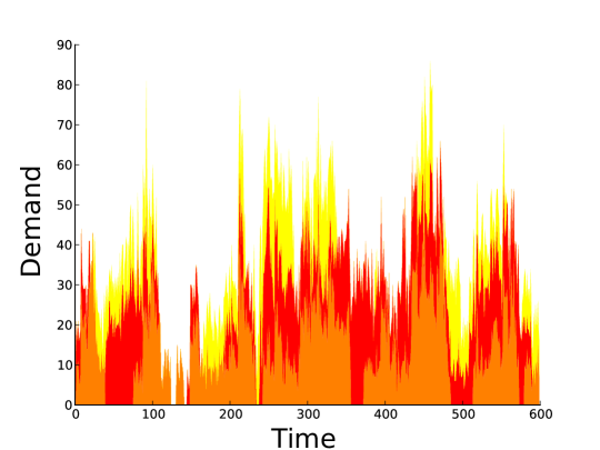
Figure 2: Sample demand realization for 3 buyers with our trace-inspired model for 600 simulated secs. Each color is a buyer’s demand.

Fig. 2 shows an example demand trace of three such buyers, each with demand 10 KBps. The pattern is bursty both at short timescales, reflecting the Poisson demand of each flow, and at longer timescales, reflecting the random flow arrival process.

The simulator supports the spq, fq, and fifo routing policies described in Section 2. Unless otherwise specified, we simulate vmm with spq routing, bks with spq routing with priorities based on resampled bids, and fixed price with fq and fifo routing. The bks resampling frequency $\mu$ is 0.2, chosen as a compromise between reducing the magnitude of rebates and not sacrificing efficiency. The results are not very sensitive to the choice of $\mu$. We show the expected allocation over 1000 allocations for bks.

We simulate truthful bidding for both bks and vmm, even though vmm is not a truthful mechanism. For memoryless demand models, this means that vmm results in the optimal allocation, acting as a benchmark for the truthful mechanisms.

6.2 Efficiency

From our analysis, we know that spq is efficient for memoryless demand models, but may not be efficient for other demand models. Here, we look at both cases, and look at the magnitude of this effect in some scenarios. We also examine the drop in efficiency due to bid resampling in bks.

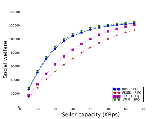
Figure 3: Efficiency of routing policies with truthful bidding. The vmm allocation is optimal in this setting, so the drop to bks is the efficiency loss due to bid resampling necessary to obtain truthfulness. spq routing for vmm and bks is much more efficient than the non-prioritized routing policies.

Fig. 3 shows the social welfare (sum of buyer and seller utilities) for a scenario with three buyers. The first two have per-KB values 10 and 4, and average demand 10 KBps each, simulating a high value and a medium value user. The last buyer has a per-KB value of only 1, but has a higher average demand–30 KBps. All buyers use the stochastic demand model described above, and we compare four different mechanisms–bks and vmm, both with spq routing and truthful bids, and fq and fifo, with a fixed price of 1. (We study the effect of changing this fixed price in the next experiment). As the seller capacity increases, the social welfare increases for all the mechanisms, until all the demand is satisfied. The demand models in this simulation are memoryless, so spq routing for vmm is optimal given that we insist on truthful bidding.

The small difference between the performance of vmm and bks is the efficiency cost of the sampling necessary for the truthfulness provided by bks. spq routing for bks is much more efficient than either of the non-prioritized fixed price policies. The difference between fq and fifo is also interesting–with fifo, the allocation is proportional to demand, so the low value, high-demand buyer gets three-fifth of the channel on average, reducing efficiency.

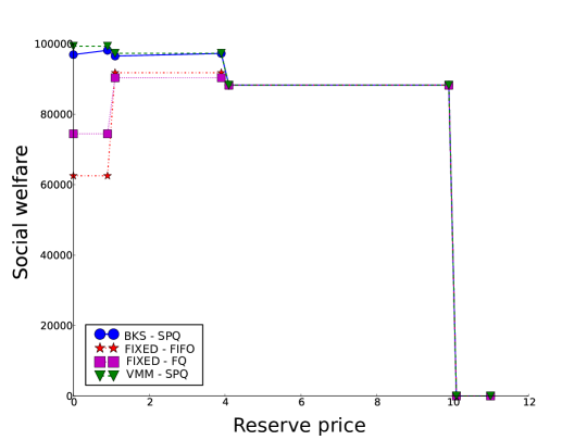
Figure 4: Efficiency of routing policies as reserve prices varies. Seller capacity is 25 KBps. Increasing the reserve price improves the efficiency of fq and fifo.

Fig. 4 shows the effect of reserve price on efficiency, in the same scenario, with seller capacity fixed at 25 KBps. Raising the reserve price slightly to avoid allocating to the lowest value buyer improves efficiency for fifo and fq. Since vmm and bks naturally prioritize high value data, raising the reserve price removes opportunities to

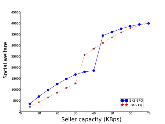
Figure 5: Efficiency for spq and fq when high value buyers leave early, and a low value buyer is impatient. Deviating to fq from spq is profitable for a range of seller capacities.

We now look at a case where a seller can profit by deviating from spq. The scenario is similar to the one above: three buyers, with per-KB values 10, 4, and 1, and average demands 10, 10, and 30 KBps. However, now the high and medium value buyers depart after 90 seconds, and the low value buyer is impatient, leaving after 60 seconds if her allocation is less than 500KB, and otherwise continuing to send for the full 600 seconds. If the seller fails to allocate at least 500KB to the third buyer in the first minute, she misses out on forwarding extra traffic later, once the two higher value bidders are gone. Fig. 5 shows the efficiency of bks with spq and fq routing. For some intermediate capacities, the value-ignorant fq routing policy is better, because it results in the low priority buyer continuing to send. Of course, if the seller knew the impatience threshold, it could use a better hybrid strategy, allocating just enough to buyer 3 to ensure she stays, and then allocating optimally to others.

6.3 Revenue pooling

Next, we study the effects of revenue pooling in align-trust, first looking at a simplified case where all sellers have the same buyer distribution, and then a more complex case where there are several seller distributions. We confirm our theoretical results, showing that the center will not have to run a deficit, and also show that pooling reduces the variance of seller revenue. Fig. 6 shows the pooled revenue vs unpooled revenue for 200 sellers from a single distribution, with seller capacity 40, buyers with per-KB values 2 and 3 and demand 10 KBps, a buyer with value 5 and demand 30 KBps, and no reserve price. In addition to the primary goal of making bks faithful for sellers, pooling drastically reduces the variance in seller revenue, with non-trivial pooled revenue for all sellers. This also shows that the tax rate for both pools is lower than 1, as predicted by the theory.

Figure 6: Effect of revenue pooling when sellers are similar.

Figure 7: Effect of revenue pooling when sellers are different.

Fig. 7 shows the pooled revenue vs unpooled revenue for 200 sellers from four different settings: seller capacities 40 or 60, and buyers with total demand 50 or 70, with higher buyer value when demand is 70. These are indicated by different markers. Note the dramatic reduction in variance of pooled seller revenue for each seller category: without revenue pooling, some sellers have negative revenue while others have very high revenue. Pooling reduces this variance, while preserving the relative ordering between seller types–sellers with higher non-pooled revenue have higher expected pooled revenue.

7 System implementation issues

Our scheme has three main components: a protocol for buyers to send bids to the sellers, a priority queueing facility for sellers to allocate bandwidth to buyer flows according to BKS, and a central server for revenue pooling and accounting. We have prototyped the first two components.

An app on the buyer’s side sends bids (along with duration of validity of the bid) to a service on the seller device. The seller device resamples the bids and uses them for allocating bandwidth, using the standard traffic control (tc) facilities in the Linux kernel (also used by Android). Specifically, upon receiving bids or updates to bids, the seller device sets (tc) filters to classify flows into one of a fixed number of priority classes based on their resampled bids, which enables the kernel to enqueue packets in the appropriate priority queue. Thus, we get efficient strict priority queuing without any kernel modifications, with the caveat that we can only use a small fixed number of queues. This implies that we need to round down the resampled bids to the nearest priority level. However, this modification preserves truthfulness since the modified allocation function is still (weakly) monotone in bids. Payments are made according to the un-rounded resampled bids.

8 Conclusion

We have introduced an approach to prioritized bandwidth access in a dynamic environment. The method succeeds in aligning incentives on both the buy-side and the sell-side of the market for a variety of stochastic demand models. While auctions can introduce an extra burden on users over charging a flat fee, they can provide for efficient allocation and the complexity can be hidden through automated bidding agents [19, 20].

There are many areas for future work. Natural extensions to the theory include expanding to more expressive demand models, and considering valuation models other than linear per byte such as value per rate and multi-dimensional valuations. The bks scheme has been extended to handle the appropriate generalization of monotonicity through a self-sampling approach [3], and the challenge would be design dynamic prioritization schemes that satisfy this cyclic monotonicity property for stochastic demand models.

We make several assumptions that are useful in analysis and developing engineering insights, even if they might not quite hold in reality. More extensive and detailed packet level simulations would be useful to study situations where our assumptions such as natural demand models and linear per-byte valuations do not hold. Analyzing real demand to determine the extent to which it confirms to our models is also future work. Finally, developing our dynamic prioritization system prototype further by designing appropriate user interfaces for eliciting buyer values, integrating with applications to allow setting traffic values, and evaluating performance such as computational overhead and energy consumption also remains to be done.

Acknowledgements: Research was sponsored by the Army Research Laboratory and was accomplished under Cooperative Agreement Number W911NF-09-2-0053.

References

- [1] Cisco Visual Networking Index: Mobile Forecast.
- [2] M. Andrews, G. Bruns, M. K. Dogru, and H. Lee. Understanding quota dynamics in wireless networks. Technical report, Bell Labs, 2013.
- [3] M. Babaioff, R. Kleinberg, and A. Slivkins. Multi-parameter mechanisms with implicit payment computation. In ACM Conf. on Electronic Commerce(EC), 2013.
- [4] M. Babaioff, R. D. Kleinberg, and A. Slivkins. Truthful mechanisms with implicit payment computation. In ACM EC, 2010.
- [5] M. Babaioff, Y. Sharma, and A. Slivkins. Characterizing truthful multi-armed bandit mechanisms: extended abstract. In ACM EC, 2009.
- [6] N. R. Devanur and S. M. Kakade. The price of truthfulness for pay-per-click auctions. In ACM EC, pages 99–106, 2009.
- [7] B. Edelman and M. Ostrovsky. Strategic bidder behavior in sponsored search auctions. Decision Support Systems, 43(1):192–198, 2007.
- [8] P. Godfrey, M. Schapira, A. Zohar, and S. Shenker. Incentive compatibility and dynamics of congestion control. ACM SIGMETRICS, June 2010.
- [9] A. V. Goldberg and J. D. Hartline. Competitive auctions for multiple digital goods. In European Symposium on Algorithms, 2001.
- [10] M. Hajiaghayi, R. Kleinberg, M. Mahdian, and D. C. Parkes. Online auctions with re-usable goods. In ACM EC, 2005.
- [11] A. Lazar and N. Semret. The progressive second price auction mechanism for network resource sharing. 8th International Symposium on Dynamic Games, Maastricht, The Netherlands, 1998.
- [12] P. Maillé et al. The progressive second price mechanism in a stochastic environment. Publication interne-IRISA, 2003.
- [13] R. B. Myerson. Optimal auction design. Mathematics of Operations Research, 6:58–73, 1981.
- [14] M. Papadopouli and H. Shen. Characterizing the duration and association patterns of wireless access in a campus. European Wireless Conference, 2005.
- [15] D. C. Parkes, M. O. Rabin, S. M. Shieber, and C. Thorpe. Practical secrecy-preserving, verifiably correct and trustworthy auctions. Electronic Commerce Research and Applications, 2007.
- [16] D. C. Parkes and S. Singh. An MDP-Based approach to Online Mechanism Design. In NIPS, 2003.
- [17] R. Porter and Y. Shoham. On cheating in sealed-bid auctions. Decis. Support Syst., 39(1):41–54, Mar. 2005.
- [18] S. Sen, C. Joe-Wong, S. Ha, and M. Chiang. A survey of smart data pricing: Past proposals, current plans, and future trends. ACM Comput. Surv., Nov. 2013.
- [19] S. Seuken, K. Jain, D. Tan, and M. Czerwinski. Hidden Markets: UI Design for a P2P Backup Application. In CHI, 2010.
- [20] S. Seuken, D. C. Parkes, E. Horvitz, K. Jain, M. Czerwinski, and D. Tan. Market User Interface Design. In ACM Conf. on Electronic Commerce, 2012.
- [21] J. Shneidman and D. Parkes. Specification faithfulness in networks with rational nodes. ACM PODC, 2004.
- [22] H. Varian and J. Mackie-Mason. Pricing the Internet. Public Access to the Internet, 1994.