Measurement of the Michel Parameter $\xi^{\prime\prime}$ in Polarized Muon Decay and Implications on Exotic Couplings of the Leptonic Weak Interaction

Abstract

The Michel parameter $\xi^{\prime\prime}$ has been determined from a measurement of the longitudinal polarization of positrons emitted in the decay of polarized and depolarized muons. The result, $\xi^{\prime\prime}=0.981\pm 0.045_{\rm stat}\pm 0.003_{\rm syst}$, is consistent with the Standard Model prediction of unity, and provides an order of magnitude improvement in the relative precision of this parameter. This value sets new constraints on exotic couplings beyond the dominant $V-A$ description of the leptonic weak interaction.

I Introduction

Normal muon decay, $\mu^{+}\rightarrow e^{+}\nu_{e}\bar{\nu}_{\mu}$, is a sensitive elementary process to probe the Lorentz structure of the charged current sector and to search for new physics beyond the Standard Model (SM) of electroweak interactions Herczeg (1986); Kuno and Okada (2001). Assuming a local, derivative free, four-fermion point interaction, invariant under Lorentz transformations, the effective muon decay amplitude can be expressed at lowest order as Fetscher et al. (1986)

$${\cal M}=\frac{4G_{F}}{\sqrt{2}}\sum_{\gamma=S,V,T\atop\epsilon,\mu=R,L}g^{\gamma}_{\epsilon\mu}\langle\bar{e}_{\epsilon}|\Gamma^{\gamma}|(\nu_{e})_{n}\rangle\langle(\bar{\nu}_{\mu})_{m}|\Gamma_{\gamma}|\mu_{\mu}\rangle$$ (1)

where $G_{F}$ is the Fermi constant and $g^{\gamma}_{\epsilon\mu}$ are the couplings associated with the scalar, vector, and tensor interactions characterized by the operators $\Gamma^{\gamma}$. Each interaction term involves electrons of chirality $\epsilon$ and muons of chirality $\mu$, whereas the indices $n$ and $m$ indicate the chiralities of the neutrinos which are uniquely determined once $\gamma$, $\epsilon$ and $\mu$ are fixed. Neutrino masses are here neglected. Within the SM, $g^{V}_{LL}=1$, and all other couplings are zero.

Observables in muon decay are conveniently expressed in terms of the Michel parameters Michel (1950) which are bilinear combinations of the couplings $g^{\gamma}_{\epsilon\mu}$ Fetscher and Gerber (1995). Most Michel parameters are known with uncertainties below the percent level Beringer et al. (2012). In particular, new results have recently been reported on the parameters ${\cal P}^{\pi}_{\mu}\xi$ Bueno et al. (2011) and $\rho$, $\delta$ Hillairet et al. (2012), for which the total errors reach respectively $(+16.8,-6.9)\times 10^{-4}$, $2.6\times 10^{-4}$, and $3.4\times 10^{-4}$. A notable exception among Michel parameters is $\xi^{\prime\prime}$, which characterizes the angular and energy dependence of the positron longitudinal polarization in polarized muon decay. This parameter has been determined only once Burkard et al. (1985a, b), yielding $\xi^{\prime\prime}=0.65\pm 0.36$, where the error is dominated by statistics.

We report here the results of an improved determination of the Michel parameter $\xi^{\prime\prime}$ deduced from a measurement of the longitudinal polarization of positrons emitted from decays of both highly polarized and depolarized muons, and discuss the implications of such a measurement in constraining exotic couplings beyond the SM that could contribute to the muon decay amplitude.

II The Longitudinal Polarization

Using the standard formalism to express the muon decay rate Fetscher and Gerber (1995); Beringer et al. (2012), assuming the SM values $\delta=\rho=3/4$, neglecting the mass of the positron and the contribution of radiative corrections Mehr and Scheck (1979), the longitudinal polarization $P_{L}$ of positrons emitted with reduced energy $x$ at an angle $\theta$ relative to the direction of the oriented muon spins (with polarization $P_{\mu}$) can be expressed as Scheck (1978)

$$P_{L}(P_{\mu},x,z)={\xi^{\prime}}\left[1+k(P_{\mu},x,z)~{}\Delta\right]$$ (2)

where $z=\cos{\theta}$, $\xi^{\prime}$ is the SM expectation for the positron longitudinal polarization, $k(P_{\mu},x,z)$ is an enhancement factor and $\Delta$ is the combination of Michel parameters

$$\Delta\equiv(\xi^{\prime\prime}/\xi\xi^{\prime}-1)\approx(\xi^{\prime\prime}-1)\,.$$ (3)

The enhancement factor $k(P_{\mu},x,z)$ determines the sensitivity to $\xi^{\prime\prime}$ embedded in $\Delta$ and is given by

$$k(P_{\mu},x,z)=\frac{P_{\mu}z\xi(2x-1)}{(3-2x)+P_{\mu}z\xi(2x-1)}\,.$$ (4)

The reduced total energy of the positron, $x=E_{e}/W_{e}$, is normalized to the decay endpoint $W_{e}=52.83$ MeV.

In the SM, the Michel parameters assume values of $\xi=\xi^{\prime}=\xi^{\prime\prime}=1$ so that $\Delta=0$ and the electron longitudinal polarization has no energy nor angular dependence. For positrons emitted from highly polarized muons, with energies close to the end-point and at backward angles relative to the muon spin, the enhancement factor takes on large values. For illustration, Fig. 1 shows the behavior of the enhancement factor for two values of the muon polarization, $P_{\mu}=0.95$ and $P_{\mu}=0.10$, assuming $\xi=1$. The dependence as a function of the variables $P_{\mu}$, $x$, and emission angle $\theta$ indicates the most favorable kinematic conditions in order to achieve a large experimental sensitivity to $\xi^{\prime\prime}$.

Figure 1: Variation of the enhancement factor $k(P_{\mu},x,\cos{\theta})$ as a function of the positron emission angle, $\theta$, for three values of the reduced energy $x$. Upper panel: for $P_{\mu}=0.95$. Lower panel: for $P_{\mu}=0.10$.

III Experimental setup

The measurement has been carried out at the $\pi$E3 beam-line of the Paul Scherrer Institute, Villigen, Switzerland. A layout of the magnetic elements of the beam-line is shown in Fig. 2. The elements are located on a vertical bending plane so that the extracted beam is 5 m higher than the primary proton beam and the muon production target. The beam line includes two bending dipoles and a series of quadrupoles. An important element for the beam purification is the velocity (Wien) filter for the separation between muons and positrons in the beam.

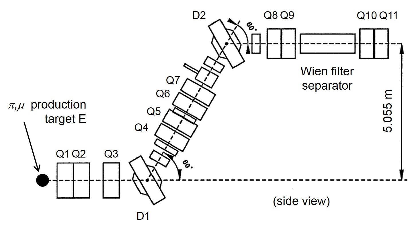
Figure 2: Vertical profile of the $\pi$E3 beam-line at the Paul Scherrer Institute showing the quadrupoles, the dipoles and the Wien filter.

III.1 Muon beam

The elements of the beam-line were tuned to select particles with momentum of 28.5 MeV$/c$, thus favoring the surface muons created from pions decaying at rest in the carbon production target. These muons are naturally backward polarized relatively to their emission direction. The initial positron contamination of the beam at this momentum was eight times larger than the muon beam intensity. The Wien filter (Fig. 2) was used to separate $e^{+}$ from $\mu^{+}$, diverting positrons from the main beam axis. At the muon implantation target (see below) the centroid of the $e^{+}$ beam profile was measured to be 16 cm away from the beam axis, far enough from the acceptance aperture of the spectrometer. After separation, the resulting $e/\mu$ contamination at the implantation target was finally 12.5%. The intensity of the muon beam was $3\times 10^{7}~{}\mathrm{s}^{-1}$ for a typical primary proton beam of 1.6 mA. After the end of the beam-line, muons were transported in air up to the implantation target over a distance of 35 cm.

III.2 Muon polarization and implantation targets

A detailed study of the residual muon polarization for muons extracted from the $\pi$E3 beam-line and implanted in a thin aluminum (Al) target was carried out in a dedicated experiment, using the technique based on the Hanle signal Possoz et al. (1979). The signal was deduced from the rates of decay positrons measured by three plastic scintillator telescopes, as a function of the beam momentum between 25 and 40 MeV$/c$. At 34 MeV$/c$, cloud muons from pion decays in flight were found to have a polarization of $-0.24$ relative to surface muons Van Hove (2000). The extrapolation of the measured cloud muon intensity and polarization towards lower momenta results in an effective beam polarization of $P^{\mathrm{Al}}_{\mu}=0.944(11)$ at 28.5 MeV$/c$ for muons implanted in the polarization-maintaining Al target Van Hove (2000). The polarization was found to be slightly larger at this momentum than at the nominal 29.8 MeV$/c$ for surface muons, probably due to energy losses in the production target. For this experiment, it is important to work at the largest possible polarization so the beam momentum was chosen to be 28.5 MeV$/c$.

In another preparatory experiment, various materials were tested for their ability to depolarize the stopped muons. Sulfur (S) was chosen since it showed strong depolarization for muons implanted with a momentum of 28.5 MeV$/c$.

Following the results of these tests, two implantation targets ($10\times 10~{}\mathrm{cm}^{2}$) of the same mass thickness ($0.405~{}\mathrm{g}/\mathrm{cm}^{2}$) were used in the final experiment, with the Al target preserving the muon polarization and the S target destroying the polarization. The targets were located in air, in a residual longitudinal stray field of about 0.1 T, generated by the magnets of the spectrometer. That field maintains the muon spin along the positron spectrometer axis.

The transport of muons inside the Wien filter separator affects the muon spins by a rotation of about $7^{\circ}$ relative to the beam axis Foroughi (2000) reducing thereby the average polarization along the spectrometer axis to $P_{\mu}^{\mathrm{Al}}=0.937(11)$.

Three plastic scintillator telescopes, two located at $\pm 90^{\circ}$ and one at $121^{\circ}$ relative to the beam direction (none is shown in Fig. 3), continuously monitored the positron rate from the muon implantation targets. The targets were tilted around their vertical axis with their planes making an angle of $75^{\circ}$ relative to the beam direction to reduce the shadowing towards the telescopes.

The dedicated muon polarization experiments clarified both the choice of the target materials and the selection of the optimal beam momentum. However, during the main experiment, the actual residual muon polarization in both targets was determined from the shape of the measured energy spectrum, as discussed in Sec. IV.9.

III.3 Positron spectrometer

The first section of the apparatus is the positron spectrometer (Fig. 3) which is located between the implantation target and the polarimeter. It is composed of three main parts: a first magnet (Filter) selecting positrons near the end-point energy, a second magnet (Tracker) where the positron momentum is measured, and a third magnet (Lens) which focuses the positrons into the polarimeter.

Extensive Monte-Carlo simulations were made using geant3 Gea , to design, optimize, and determine the operating conditions of the spectrometer Van Hove (2000). All three spectrometer magnets have cylindrical symmetry and generate solenoidal fields. The field intensities, on axis at the center of the magnets, were 1.86, 2.66, and 0.80 T, respectively, for the “Filter”, “Tracker” and “Lens”.

The Filter magnet selects positrons with energies larger than 44 MeV, emitted into a cone defined by $163^{\circ}<\theta<177^{\circ}$ relative to the magnet axis, which also defined the average muon polarization axis. The magnetic field was produced by a split-pair superconducting coil. The warm bore was filled with copper scrapers and collimators, shaped so that only energetic positrons emitted into the above given angles could pass through. These obstacles also stop the remaining 28.5 MeV/c positrons that contaminated the muon beam.

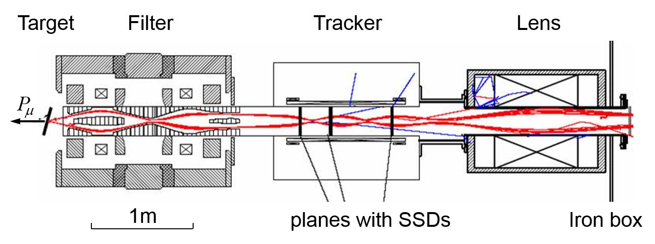
Figure 3: (Color online) General view of the three magnets that are assembled into the spectrometer. The Filter accepts only high energy decay positrons, stopping the remainder. The Tracker is used for energy analysis, and the Lens transports the positrons to the polarimeter (Fig. 6). The red lines are tracks for 50 MeV$/c$ positrons generated via Monte-Carlo simulation and the blue lines are secondary particles. The arrow on the implantation target shows the average direction of the muon polarization.

The magnetic field in the Tracker was provided by an 81 cm long superconducting coil (including two trim coils) generating a uniform field over a large volume. The 1 m long by 20 cm diameter warm bore hosted three planes of double-sided position-sensitive Si strip detectors (SSD) to measure the positron momentum. Inside the Tracker magnet, decay positrons make at least one full turn of their helix-shaped trajectories. The positron momentum is determined from the intersections of the tracks with the three planes of SSDs.

Each plane contains four $300~{}\mu\mathrm{m}$ thick ($60\times 60~{}\mbox{mm}^{2}$) SSDs mounted on an aluminum support as indicated in Fig. 4. Each detector has 60 independent strips per side resulting in a position resolution of 1 mm in both horizontal and vertical directions.

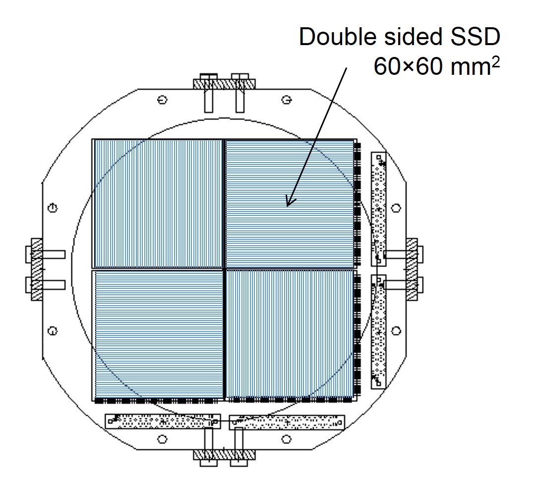
Figure 4: (Color online) Front view of the arrangement of four SSDs on the frame of one of the three planes of detectors located inside the Tracker (Fig. 3). The boards with the front-end electronics were connected perpendicular to these planes.

The distance between the first and second planes was $z_{21}=21$ cm and the distance between the second and the third planes was 42 cm. With this geometry, the radial and longitudinal components of the momentum are given by Van Hove (2000)

$$p_{r}=\frac{eBd^{2}_{21}}{\sqrt{4d^{2}_{21}-d^{2}_{32}}}\,.$$ (5)

and

$$p_{z}=\frac{eBz_{21}}{2\arccos{\left[-d_{32}/(2d_{21})\right]}}\,,$$ (6)

where $e$ is the electric charge of the positron, $B=2.66$ T is the magnetic field intensity and $d_{ij}=\sqrt{(x_{j}-x_{i})^{2}+(y_{j}-y_{i})^{2}}$ is the projection on the vertical $(x,y)$ plane of the distance between hits in the SSD planes $i$ and $j$.

Monte-Carlo simulations indicated that the energy resolution of the spectrometer is 1.15(4) MeV FWHM over the selected energy range. The fits to real data are fully consistent with this value. Details about the design, the electronics, and performance of the spectrometer can be found in Ref. Van Hove (2000). In particular, both positron transmission rates and momentum distribution shapes downstream from the spectrometer have been checked during preliminary tests and were found to be consistent with the Monte-Carlo simulations Van Hove (2000).

Figure 5 shows two energy spectra, after software cuts (see below), for positrons emitted from the Al and S targets. For comparison purposes the spectra have been normalized to their respective maxima. The reduced event rate from the Al target, due to the muon polarization being maintained, is clearly visible at higher energies. The points show experimental data and the lines are calculated distributions including the spectrometer transmission function.

Figure 5: Typical normalized positron energy spectra as deduced from the momentum measurement with the SSD located inside the Tracker magnet for positrons transmitted through the spectrometer. The distributions correspond to muons implanted in the Al target (left curve) and S target (right curve). The full circles are for positrons which underwent Bhabha scattering in the polarimeter and the open circles for positrons which annihilated in flight. The solid lines show calculated shapes assuming muon polarizations $P_{\mu}^{\mathrm{Al}}=0.937$ and $P_{\mu}^{\mathrm{S}}=0.382$.

Finally, the Lens magnet guides transmitted positrons into the polarimeter so that the positron trajectories become essentially parallel to the spectrometer axis at the location of the magnetized foils used for the polarization analysis.

III.4 Polarimeter

The determination of the positron longitudinal polarization was made using the spin dependence of Bhabha scattering (BHA), $e^{+}+e^{-}\rightarrow e^{+}+e^{-}$ Bincer (1957); Ford and Mullin (1957), and annihilation in flight (AIF), $e^{+}+e^{-}\rightarrow\gamma+\gamma$, McMaster (1960); Page (1957); Fetscher (2007) processes. Data for both processes can be recorded simultaneously, due to the similar kinematics which, in principle, offers an additional check on possible systematics since the two processes have analyzing powers with opposite signs Corriveau et al. (1981).

Incoming positrons were detected at the entrance of the polarimeter (Fig. 6) by a coincidence between two plastic scintillators noted PS1 and PS2. The position at the entrance was determined with the first out of five multi-wire proportional chambers, MWPC(1), located behind the plastic scintillators.

Two Vacoflux-50 foils ($75\times 15~{}\mathrm{cm}^{2}$) mounted on a loop around a magnetized ARMCO alloy yoke produced electrons with a polarization $P_{e}$ oriented in the plane of the foils. Due to the loop where the foils are mounted, the polarization on the two foils have opposite directions. During operation, the foils were first magnetized up to saturation by two coils wound around the yoke and then left magnetized at their remnant fields.

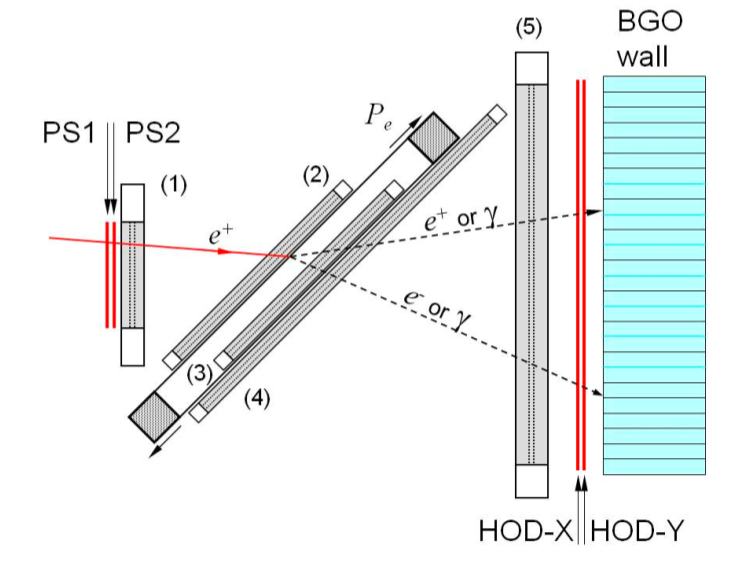
Figure 6: (Color online) Top view of the positron polarimeter with tracings of a scattering event occurring in the first magnetized foil of the Vacoflux foil loop. The plastic scintillators (in red) PS1 and PS2 detect incoming positrons, while the hodoscope scintillators HOD-X and HOD-Y in coincidence with the segmented BGO determine the scattering type. The MWPC are labeled (1)–(5). The Vacoflux foil loop mounted around the yoke provides polarized electrons ($P_{e}$).

For their construction, the foils and the yokes were heated to $820^{\circ}$C for about 6 hours in an N₂ atmosphere and then slowly cooled during 10 hours in the presence of an external field of 38 Gauss Vacuumschelze (2002). Such treatment generates a sharp hysteresis curve Morelle (2002) allowing the measurement during the main experiment to be performed without current in the coils following foil magnetization.

The induced magnetic field over the $36\times 15~{}\mathrm{cm}^{2}$ active surfaces was 1.910(5) T. The foil thickness over the active regions was optimized to 0.75(1) mm following detailed Monte-Carlo simulations Morelle (2002). From the gyromagnetic factor of the alloy and the foil magnetization, the electron polarization along the foil direction was estimated to be $P_{e}=6.88(5)$%. Due to the foil orientation by 45^∘ relative to the beam axis, the effective electron polarization along the spectrometer axis was then $P_{\mathrm{eff}}=4.86(3)$%. As explained in Sec. IV.8, it is not necessary to accurately know the value of the effective electron polarization. The foils were sandwiched between three wire chambers, MWPC(2)–(4), used to locate the vertex where the AIF or BHA scattering occurred. The two foils, their support yoke, as well as the three wire chambers, can be rotated as a unit about the vertical axis allowing the orientation to be changed by $\pm 45^{\circ}$ relative to the beam axis.

The polarimeter is completed by a fifth MWPC, a hodoscope (HOD–X and HOD–Y) and a calorimeter. The hodoscope consists of two planes of plastic scintillators, each having seven slices (90 mm wide and 3 mm thick) of variable lengths such as to cover the hexagonal front face of the calorimeter (Fig. 7). Each panel of the hodoscope was read by a single photomultiplier.

The calorimeter wall consists of 127 BGO crystals, 20 cm long, of hexagonal section. This set of detectors was used in the same geometry as in a previous measurement of the transverse polarization of positrons emitted from polarized muons Danneberg et al. (2005). The BGO wall was surrounded by a thermal shield to stabilize the inner temperature within $\pm 2^{\circ}\mathrm{C}$. In order to limit temperature variations, the high voltage dividers for the BGO photomultipliers were located outside the thermal shield. Details about the geometry, temperature stabilization, photomultipliers, readout electronics and performance of the calorimeter can be found in Ref. Barnett et al. (2000). Two pairs of plastic scintillators panels (Fig. 7), $1600\times 160\times 12~{}\mathrm{mm}^{3}$ in size for the top pair and $1220\times 160\times 12~{}\mathrm{mm}^{3}$ for the bottom pair, were located above and below the BGO wall to detect cosmic rays. Each panel for cosmic rays detection was read with two photomultiplier tubes, one at each end of the scintillator.

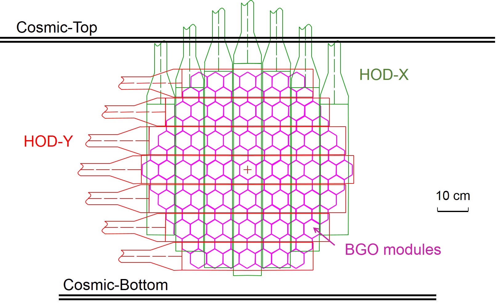
Figure 7: (Color online) Front view of the hodoscope and the calorimeter showing the position of the scintillator detectors: HOD-X (in green), HOD-Y (in red) and top and bottom cosmic rays telescopes (in black) relative to the hexagonal front face of the BGO modules of the calorimeter (in magenta).

The entire polarimeter was located inside a $3\times 3\times 1.8~{}\mathrm{m}^{3}$ iron box, partly indicated on Fig. 3, to shield the analyzing Vacoflux foils and the (otherwise unshielded) calorimeter photomultipliers from the stray field generated by the spectrometer magnets. The residual field intensity inside the iron box was smaller than 0.4 mT.

III.5 Signal treatment and data acquisition

Due to the different time responses of the various detectors, three types of signal readout systems were used: one for the plastic scintillators (target monitor telescopes, polarimeter entrance scintillators, hodoscopes, and cosmic muon detectors), another for the SSD and MWPC signals, and a third for the BGO modules. The fast plastic scintillator signals were treated with standard discriminators and coincidence units to construct the logic signals used in the subsequent triggering decisions.

The BGO detector readout used a set of Lecroy Research Systems (LRS) Fera modules, LRS-4300B analog-to-digital converters for the energy information and LRS-3377 time-to-digital converters for the time information. The gain stability of the BGO crystals was controlled with independent LED pulsers located on each module and producing pulses of three different amplitudes. The LEDs were triggered by an external clock at 10 Hz.

The SSD and MWPC signals were read using VA-Rich chips (from IDE-AS). A single chip can read and store signals from 64 channels so that one chip was used to read and store the 60 channels (one side) of each silicon detector. To collect the analog data of all $3\times 4$ double-side strip detectors, 24 VA-Rich were used. When triggered, a V551B CAEN VME module drove all VA-Rich chips in parallel, first with the hold signal to lock in the event of interest, then with the multiplexer signals to read the data into V550 CAEN modules where the signals were digitized and noise subtracted. The data was then transferred to the acquisition computer. A similar system with 15 VA-Rich chips was used for the MWPC readout. The full reading time per event took roughly $700~{}\mu\mathrm{s}$.

After shaping and discrimination, the logic indicating any of several different events (detailed below) was realized with ALTERA programmable logic gate arrays. All plastic scintillators as well as the combined BGO signals entered the trigger logic whereas data from the SSD and the MWPC were read only when required, based on the trigger type. To reduce pile-up events which could lead to the misidentification between the signals of an incoming positron and those of outgoing particles, an updated dead time of $3~{}\mu\mathrm{s}$ was imposed on the trigger logic once a positron was detected at the entrance of the polarimeter. The fast acquisition system was based on a vxWorks front-end hosted in CAMAC and VME combined with back-end software developed by the group at Louvain–la–Neuve.

A slow control system, based on LabView, was used to set and monitor other parameters of the apparatus such as: i) the foil magnetization current and the sequence for reversing the foil magnetization; ii) the high voltage of the plastic scintillators and BGO detectors; iii) the number and the amplitude of each of the LED signals sent to the BGO modules; and iv) the measurement and control of the temperature inside and outside the BGO thermal shield. The current for the loop magnetization was reversed by the slow control system after every one-hour run. Data with the depolarizing S target was taken for 12 hours after every two days of measurement with the polarization-maintaining Al target. The magnetized foils together with MWPC(2)–(4) were rotated between $+45^{\circ}$ and $-45^{\circ}$ every four days.

The data acquisition included eight mutually exclusive triggers running simultaneously. Table 1 gives their names and comparative rates for polarized and unpolarized muons. The trigger for the primary AIF and BHA events, or for noninteracting Michel (MIC) positrons was generated by an incoming positron by combining three signals: 1) the coincidence (PS1$\cap$PS2) providing the time-zero reference for the event; 2) the signals from HOD–X, HOD–Y, and MWPC(5) which entered the trigger decision via a hardware selection of the multiplicity of the detectors: 0 for events identified as AIF, 2 for BHA, and 1 for the most frequent MIC events arising from positrons simply crossing the polarimeter; and, 3) a fast summed amplitude signal from the BGO giving the total energy deposited in the calorimeter, with a threshold set at 30 MeV. The MIC triggers were prescaled by a factor 50 to reduce the load on the data acquisition system. LED signals and cosmic muons crossings the BGOs were additional triggers. The triggers from the plastic scintillator telescopes located around the muon implantation target, were independent from those of events in the polarimeter and were used for on-line monitoring of the muon beam intensity and polarization.

Table 1: Average event rates (in $\mathrm{s}^{-1}$) for each kind of trigger at a typical primary proton beam current of 1.6 mA. The bottom line indicates the corresponding acquisition dead-time, which was mostly due to the conversion and reading time of the V550–V551B modules.

Trigger source	Al target	S target
Annihilation (AIF)	64	160
Bhabha (BHA)	79	205
Michel/50 (MIC)	47	122
Cosmic	0.5	0.5
LED	8	8
Telescope($121^{\circ}$)/100	19	16
Telescope($+90^{\circ}$)/100	12	12
Telescope($-90^{\circ}$)/100	14	14
Dead Time	15%	34%

IV Data Analysis

A total of 501 data sets, each of about one hour duration, have been collected during the experiment. From this set, numerous runs correspond to tests made at the beginning and at the end of the experiment. From the remaining files, 255 runs were selected by the filters for which the proton beam intensity was stable during the measurement and all components of the apparatus and electronics operated without fault. The data analysis was applied to this final set of files which contained comparable statistics for the different configurations.

IV.1 Calibration of the BGO modules

The energy calibration of the BGO modules was performed using both MIC and cosmic events. The momentum of a MIC event is first measured by the SSD tracker following Eqs. (5) and (6). The energy of the same MIC positron as measured in the calorimeter results from its convolution with the polarimeter transmission function. That function is determined via Monte-Carlo simulation and includes the energy losses in the plastic scintillators, in the MWPCs, and in the Vacoflux foils.

Cosmic ray muons deposit a rather constant amount of energy in each module, and the trajectory of a cosmic event can be easily reconstructed when five or more BGO modules are hit. With fewer involved modules, the determination of the energy loss per length becomes difficult, in particular in the outer region of the wall. Because of that difficulty, the BGO modules were calibrated only once using a large set of cosmic ray events collected during a period when there were no muons from the beam.

The module gain stability was monitored with LED signals of three different amplitudes. The three LED peak positions were observed to drift by up to 10% relative amplitude over the 25 day duration of the effective measurement. Such drift was not caused by variations in the LED light output since correlated drifts were observed for the MIC spectra centroid as seen by the BGO wall. By deconvoluting the measured distribution from the polarimeter transmission function, the average energy resolution of the BGO wall was found to be 10.4 MeV FWHM at 42 MeV.

IV.2 Tracking efficiencies

The efficiencies of the MWPC and the plastic-scintillator hodoscope have also been determined using MIC events. Reconstructed tracks for “perfect” MIC events contain only one hit in each plane of each MWPC as well as a single hit on the plastic scintillator hodoscope, with one signal on the vertical and one on the horizontal directions. The detector inefficiencies are found by comparing the rates of such “perfect” Michel events to those where one of the expected hits is missing.

Among the ten MWPC wire planes, the smallest efficiencies were consequently found to be 96.1% for the plane giving the horizontal position in MWPC(4) and 97.3% for the plane giving the vertical position in MWPC(3). All other planes had efficiencies larger than 99.0%.

Because the hodoscope scintillators do not overlap each other, the surface covered by the scintillators has long thin gaps both horizontally and vertically (Fig. 7). The hodoscope efficiency was 95.9% horizontally and 98.7% vertically, roughly in accordance with the $~{}2$–$3$ mm separation between the 90 mm wide scintillator strips. This separation was caused by the individual scintillator light-tight wrapping. By extrapolating the MWPC track information to the hodoscopes for tracks with missing hodoscope hits, it was clearly shown that the missing hits corresponded to the small gaps between adjacent scintillators.

IV.3 Data selection

The AIF and BHA events have a two-body final state following the reactions in one of the Vacoflux foils. In the laboratory frame, the opening angle, $\phi$, between the two outgoing particles can be determined from the event topology, using the position information from the MWPCs. The relation between this angle and the total energies, $E_{1}$ and $E_{2}$, of the outgoing particles having both a rest mass $m$, is obtained from simple kinematics

$$\cos{\phi}=\frac{E_{1}E_{2}+m^{2}c^{4}-m_{e}c^{2}(E_{1}+E_{2})}{\sqrt{E_{1}^{2}-m^{2}c^{4}}\sqrt{E_{2}^{2}-m^{2}c^{4}}}.$$ (7)

For BHA events, $m=m_{e}$, where $m_{e}$ is the electron mass, whereas for AIF events ($m=0$) this equation simplifies to

$$\cos{\phi}=1-m_{e}c^{2}\frac{E_{1}+E_{2}}{E_{1}E_{2}}.$$ (8)

It is convenient to use Eqs. (7) and (8) for a kinematic identification of the signal for the scattered events in a two dimensional histogram plotting the ratio, $E_{1}/E_{2}$, between the smallest and the largest of the two energies versus $\cos{\phi}$. Such signature was clearly visible for AIF events (Fig. 8) but not for BHA events, possibly due to scattering in matter between the foils and the calorimeter and to the contribution of misidentified background.

Within the energy interval selected in the experiment, BHA events following Eq. (7) are expected to have a very similar signature to the one observed for AIF events in the two-dimensional distribution of Fig. 8, since the electron rest mass is small compared to the total energies of the outgoing electron and positron. Consequently, for the uniformity of treatment, the same kinematic cut was applied to BHA and AIF data as indicated by the line in Fig. 8, to separate the signal from background events visible at small angles. Additionally, an energy cut required both $E_{1}$ and $E_{2}$ to be each larger than $6$ MeV, and an upper limit of $(E_{1}+E_{2})<70$ MeV was also imposed to reject accidentally summed events.

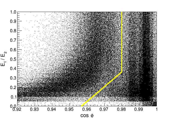
Figure 8: (Color online) Two-dimensional distribution of events selected by the AIF trigger plotted as a function of the measured $\cos{\phi}$, where $\phi$ is the angle between the two photons in the laboratory system and of the ratio $E_{1}/E_{2}$ between the smallest and the largest energies of the photons. The sweeping distribution at the left corresponds to AIF events following Eq. (8). The line shows the cut limit applied to both AIF and BHA events.

After passing checks of calorimeter gain stability and calibration, the off-line analysis proceeded in three steps: i) the positron momentum is determined from the hits of the SSD located inside the Tracker magnet; ii) evaluations are made of the energies and barycenter positions of the clusters created by the two reaction products as detected by the calorimeter; and iii) the event vertex and scattering foil is reconstructed from the MWPCs data. No background subtraction has been performed on the selected events.

IV.4 Super-ratios

For each scattering process (BHA and AIF) the events were sorted into one of $2^{4}$ different types according to the experimental conditions of the four main measurement parameters: i) the foil where the scattering occurred (1st or 2nd); ii) the current polarity for the Vacoflux loop magnetization ($\pm$: positive or negative); iii) the magnetized foil orientation relative to the beam axis ($\pm 45^{\circ}$); and iv) the implantation target (Al for polarization maintaining, or S for depolarizing).

For a given run, the number of events originating from the 1st and 2nd foils, $y_{1}$ and $y_{2}$, are measured simultaneously. It is then convenient to take the ratio of those numbers to avoid the use of an external normalization. These ratios are the primary information extracted from each run and are noted $r^{\pm}_{\alpha}=y_{1,\alpha}^{\pm}/y_{2,\alpha}^{\pm}$, where $\pm$ indicates the magnetization-current polarity and $\alpha$ stands for the eight remaining experimental conditions.

Under magnetization current-polarity reversal, effects associated with the electron polarization do change sign but effects from detector geometry do not. From the ratios $r^{\pm}_{\alpha}$ introduced above one then defines the “super-ratios” $s_{\alpha}$ by

$$s_{\alpha}=\frac{r^{+}_{\alpha}-r^{-}_{\alpha}}{r^{+}_{\alpha}+r^{-}_{\alpha}}\,.$$ (9)

As will be shown in Sec. IV.5, differences in solid angles $\omega_{i,\alpha}^{\pm}$ from foils $i=1$ and 2 relative to the polarimeter detectors as well as effects due to different incident positron intensities on the foils cancel in the super-ratios under the assumption that $\omega_{1,\alpha}^{+}\omega_{2,\alpha}^{-}=\omega_{1,\alpha}^{-}\omega_{2,\alpha}^{+}$.

Since the data are finally analyzed as a function of the energy obtained from the positron momentum as measured by the SSD Tracker, the super-ratios are sorted into 20 energy bins from 45 to 55 MeV. This energy sorting results in rather small statistics per bin within each run. Moreover the combination of selected runs having opposite polarization currents to form the super-ratios could possibly induce a bias. Consequently, the statistics from all the 255 runs has been grouped and sorted for the different configurations. This generates $2^{5}$ summed event vectors of 20 energy bins, corresponding to the different running conditions (foil number, current polarity for the magnetization, orientation of the magnetized foil, implantation target Al or S) and event type (AIF or BHA).

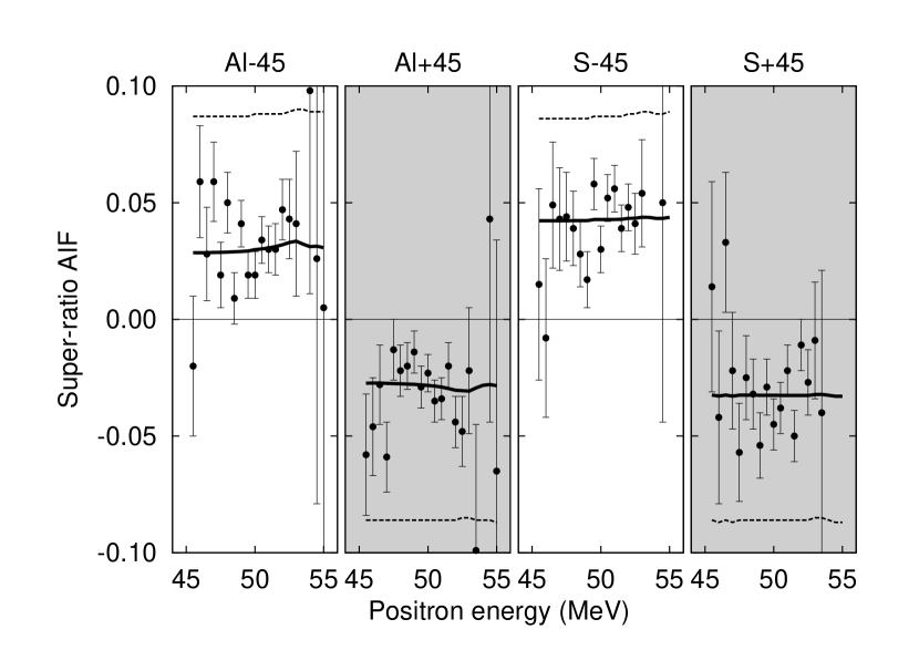
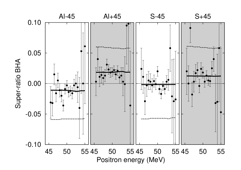
Figure 9: Experimental super-ratios, Eq. (9), for the two targets and the two orientations of the scattering foils as a function of the positron energy for AIF (upper panel) and BHA (lower panel). The dotted lines show the values of the function $\varphi(A^{\pm}_{i,\alpha})$ which is the super-ratio calculated from the analyzing power assuming a positron polarization $P_{L}=1$ (Sec. IV.6). The solid lines correspond to the fit of the super-ratios (Sec. IV.8).

The eight sets of super-ratios calculated for each of the two processes, the two target types, and the two orientations of the magnetized foil are shown in Fig. 9 as a function of the positron energy. The sign inversion of the asymmetries under the $\pm 45^{\circ}$ rotations of the magnetized foils is clearly visible. The asymmetries for AIF are seen to be larger than for BHA and with opposite signs as expected from the analyzing powers of these processes Corriveau et al. (1981).

IV.5 Analyzing powers

In order to estimate the maximal values expected for the super-ratios and to study the energy dependence of the analyzing powers, the measured ratios of events between foil 1 and 2 can be expressed as a function of solid angles, the longitudinal polarization, and analyzing powers:

$$r^{\pm}_{\alpha}=\frac{\omega^{\pm}_{1,\alpha}(1+P_{L}A^{\pm}_{1,\alpha})}{\omega^{\pm}_{2,\alpha}(1+P_{L}A^{\pm}_{2,\alpha})}$$ (10)

where $A^{\pm}_{i,\alpha}$ are the analyzing powers for each configuration and type of process and include the relative sign associated with the selected geometry and scattering process. Again, subscript $i=(1,2)$ refers to the Vacoflux foil in which the scattering occurred, and $\alpha$ indexes the other eight experimental conditions associated with the foil orientation, the two scattering processes and the implantation target.

The analyzing powers, $A^{\pm}_{i,\alpha}$, were extracted by using the kinematic variables from experimental data and the cross sections of the scattering processes as calculated from quantum electrodynamics (QED). For each scattering event, $l$, the incoming positron energy and the kinematics of the outgoing particles are used to compute the corresponding raw analyzing power, $(a_{p})_{l}$, of the associated process (BHA Ford and Mullin (1957), AIF Page (1957); McMaster (1960)), assuming $P_{L}=1$. The MWPC tracking data are used to determine the angle, $\theta_{s}$, between the direction of the electron spin in the struck Vacoflux foil and that of the momentum of the incoming positron, thus providing a weight factor, $(\cos{\theta_{s}})_{l}$, for $(a_{p})_{l}$. Table 2 gives the absolute value of the mean and RMS for the $a_{p}$ and $a_{p}\cos{\theta_{s}}$ distributions obtained from all events and configurations for each of the two processes (AIF or BHA). In practice, $\theta_{s}$ is very close to $45^{\circ}$ (the mean is $44.3^{\circ}$ for AIF and $44.6^{\circ}$ for BHA) since the direction of incidence of the positrons is almost parallel to the spectrometer axis.

Table 2: Absolute mean and standard deviations of the distributions of the calculated analyzing powers, $a_{p}$, and of the projections $a_{p}\cos{\theta_{s}}$.

	$a_{p}$		$a_{p}\cos{\theta_{s}}$		Number of
Process	Mean	RMS	Mean	RMS	events
AIF	0.88	0.022	0.63	0.066	$1\,564\,835$
BHA	0.59	0.15	0.42	0.11	$2\,313\,549$

Like for the super-ratios, the analyzing powers and their projections were sorted into 20 energy bins and further classified by the $2^{4}$ experimental conditions for the two scattering processes. The energy distributions resulting from this sorting were then multiplied by the electron polarization $P_{e}$ in the Vacoflux foils, and each energy bin was normalized by the number, $n$, of values used in that bin. These operations can be summarized by the following expression for the calculated analyzing power at each energy bin

$$A^{\pm}_{i,\alpha}=\left[\frac{P_{e}}{n}\sum_{l=1}^{n}(a_{p})_{l}(\cos{\theta_{s}})_{l}\right]^{\pm}_{i,\alpha}\,.$$ (11)

The distributions of the analyzing power corresponding to the negative magnetization current are shown in Fig. 10 for AIF and BHA events. The distributions associated with the positive magnetization current are not shown since they behave similarly except for their global sign reversal compared with the negative magnetization.

The main conclusion from this study is that the analyzing powers of the two processes as calculated within QED are, to a sufficient approximation, constant over the measured interval of the positron energy. In particular, the asymmetries do not display any significant variation towards the end-point energy.

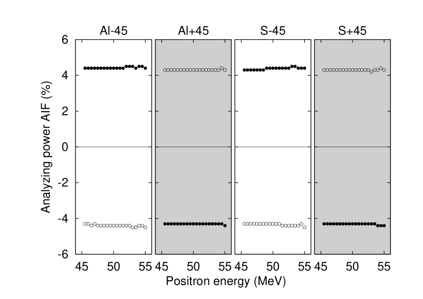
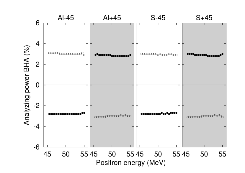
Figure 10: Calculated analyzing powers $A^{-}_{i,\alpha}$, corresponding to the negative magnetization current, as a function of the positron energy for AIF events (upper panel) and BHA events (lower panel). The open (closed) circles are for events from scattering foil 1 (2). The values for the positive magnetization current, $A^{+}_{i,\alpha}$, have a similar trend but with opposite signs and are not shown.

IV.6 Longitudinal polarization

The super-ratios in Eq. (9) can be expressed as a function of the positron longitudinal polarization by using Eq. (10), and assuming that $\omega_{1,\alpha}^{+}\omega_{2,\alpha}^{-}=\omega_{1,\alpha}^{-}\omega_{2,\alpha}^{+}$:

$$s_{\alpha} = P_{L}\frac{f_{1}(A^{\pm}_{i,\alpha})+P_{L}f_{2}(A^{\pm}_{i,\alpha})}{2{+}P_{L}f_{3}(A^{\pm}_{i,\alpha}){+}P^{2}_{L}f_{4}(A^{\pm}_{i,\alpha})}$$ (12)

$$= P_{L}\varphi(A^{\pm}_{i,\alpha},P_{L})\,.$$ (13)

The functions $f_{j}(A^{\pm}_{i,\alpha})$ have the following dependences on the analyzing powers

$$f_{1} = (A^{+}_{1}+A^{-}_{2})-(A^{-}_{1}+A^{+}_{2})$$ (14)

$$f_{2} = A^{+}_{1}A^{-}_{2}-A^{-}_{1}A^{+}_{2}$$ (15)

$$f_{3} = (A^{+}_{1}+A^{-}_{2})+(A^{-}_{1}+A^{+}_{2})$$ (16)

$$f_{4} = A^{+}_{1}A^{-}_{2}+A^{-}_{1}A^{+}_{2}$$ (17)

where the subscripts $\alpha$ were omitted for clarity. In order to estimate the remaining dependence of the function $\varphi(A^{\pm}_{i,\alpha},P_{L})$ on the positron longitudinal polarization, the function was computed for the extreme values $P_{L}=0$ and $P_{L}=1$. For all values of the reduced energy within the selected energy interval, this comparison shows a variation $0.998\leq\varphi(A^{\pm}_{i,\alpha},1)\;/\varphi(A^{\pm}_{i,\alpha},0)\leq 0.999$ which can be neglected at the current level of precision. The polarization $P_{L}$ in $\varphi(A^{\pm}_{i,\alpha},P_{L})$ was then fixed to $P_{L}=1$. Equation (13) then becomes a linear function of the positron longitudinal polarization:

$$s_{\alpha}=P_{L}\varphi(A^{\pm}_{i,\alpha})\,,$$ (18)

where the dependence of $\varphi$ on the positron polarization has been omitted.

Since the analyzing powers $A^{+}_{i}$ and $A^{-}_{i}$ are of similar magnitude but have opposite signs we have $f_{3}\approx 0$ in Eq. (16). Next, since the linear terms in the analyzing powers dominate the super-ratio given in Eq. (12), the leading term is given by the function $f_{1}$ so that, within the accuracy of this experiment, $\varphi(A^{\pm}_{i,\alpha})$ is approximately equal to $A^{+}_{1,\alpha}+A^{-}_{2,\alpha}\approx 2A^{+}_{1,\alpha}$.

The functions $\varphi(A^{\pm}_{i,\alpha})$ are superimposed on the data in Fig. 9 for the eight ${\alpha}$ configurations. The differences between the average measured super-ratios and the calculated functions are discussed in Sec. IV.8.

IV.7 Enhancement factors

For each target type ($T=$Al or S), the positron transmission rate through the spectrometer varies with the positron energy and emission angle as

$$n^{T}(x)\propto\int_{\Omega}\!\left[F(x)+\xi P^{T}_{\mu}G(x,z)\right]d\Omega\,$$ (19)

where $F(x)=x^{2}(3-2x)$, $G(x,z)=x^{2}z(2x-1)$ and the integral is performed over the angular acceptance of the spectrometer. The equations for the two targets can be combined to form the ratio,

$$\frac{n^{\mathrm{Al}}(x){-}n^{\mathrm{S}}(x)}{n^{\mathrm{Al}}(x)}=\frac{(P^{\mathrm{Al}}_{\mu}-P^{\mathrm{S}}_{\mu})\xi\int_{\Omega}\;G(x,z)d\Omega}{\int_{\Omega}\;\left[F(x)+\xi P^{\mathrm{Al}}_{\mu}\;G(x,z)\right]d\Omega}.$$ (20)

The factor $x^{2}$, which enters $F(x)$ and $G(x,z)$, cancels in the expression given in Eq. (4) extracted from the double differential decay rate. The right-hand side of Eq. (20) contains then the kinematic factor that appears on the right-hand side of Eq. (4). Consequently, the actual enhancement factors can be expressed as a function of measured quantities, after integrating the rates over the spectrometer acceptance. For each of the two targets $T$ we have

$${k(P^{T}_{\mu},x)}=\frac{n^{\mathrm{Al}}(x)-n^{\mathrm{S}}(x)}{n^{T}(x)}\frac{P^{T}_{\mu}}{(P^{\mathrm{Al}}_{\mu}-P^{\mathrm{S}}_{\mu})}\,.$$ (21)

This expression is composed of two factors: the first is determined from the experimental yields and is strongly energy dependent; the second is determined from the muon polarization in the target and is energy and geometry independent. The first factor could potentially differ for each of the $\alpha$–labeled configurations since the geometry of the selected events can vary. For that reason the transmitted positrons selected for the determination of the enhancement factors are those that undergo either AIF or BHA scattering, chosen independently of the foil in which the scattering process took place but otherwise sorted following the eight $\alpha$ configurations and the two magnetizing currents.

Figure 11: Energy dependent part of the enhancement factor in Eq.(21) as deduced from the rates of AIF events (upper panel) and BHA events (lower panel) selected for the eight $\alpha$ configurations presented in Fig. 9. The enhancement factors for the two magnetization currents were averaged. The dotted lines between the points are to guide the eye.

Since the energy dependent part of the enhancement factors for the two current polarities are very close, the mean value, $k_{\alpha}$, has been taken as the enhancement factor used in the final fit. The results are shown in Fig. 11. The reduction of the enhancement factor observed at high energy was anticipated by Monte-Carlo simulations performed during the design of the spectrometer Van Hove (2000) and is due to the finite acceptance and momentum resolution.

We stress an important aspect of this experiment using both polarized and depolarized muons, namely the fact that the enhancement factors are extracted from the transmitted positron rates measured with the Al and S targets, as well as from a simple determination of the corresponding muon polarization. Since the very same device is used for the energy measurement and an identical energy binning is applied to the extraction of the super-ratios and of the enhancement factors, the data analysis does not require an accurate absolute energy calibration of the spectrometer. Moreover, since the measurement of the longitudinal polarization is differential, as a function of the positron energy, the measurement does not require either an accurate determination of the absolute analyzing power of each scattering process selected by the polarimeter.

IV.8 Fits

According to Eq. (18), the super-ratios are proportional to the positron polarization, $P_{L}$. The dependence of $P_{L}$ as a function of $\Delta$ is given by Eq. (2) and is driven by the enhancement factors shown in Fig. 11.

As is visible in Fig. 9, the amplitudes of the measured super-ratio are smaller than the maximal possible amplitudes as given by the calculated functions ${\varphi(A^{\pm}_{i,\alpha}})$. Two main sources have be considered to explain such differences: 1) A reduction could arise from a smaller magnetization in the Vacoflux foil. A smaller electron polarization in the foil would reduce the effective analyzing power. If this were the only effect responsible for the observed reduction, the factor would then be the same for AIF and BHA processes. However, this is not observed to be the case in the super-ratios (Fig. 9). In any event, such a reduction of the super-ratios due to a non-saturation of the foils has no dependence on the positron energy; 2) The contribution of background events remaining after the software cuts and the misidentifications of events due to tracking inefficiencies of the MWPC and detection inefficiencies in the hodoscope tend to reduce the amplitude of the super-ratios. Although, strictly speaking, the probability for a positron to produce background events, such as a double bremsstrahlung, is naturally energy dependent, such dependence varies smoothly over the energy window considered in this experiment. Neither of these two sources appears to be able to mimic a strong energy dependence like the one shown by the enhancement factors.

As a next step, in order to search for a possible energy dependence of the longitudinal polarization, the super-ratios have then been fitted by the function,

$$s_{\beta}(x)=a_{\beta}P_{L}(x)\varphi(A_{\alpha})+b_{\beta}\,,$$ (22)

where $a_{\beta}$ is a common attenuation factor for each pair of configurations $\alpha$ associated with the $\pm 45^{\circ}$ orientations of the foils, and $b_{\beta}$ is an offset for the same pair of configurations. The central assumption of this model is that the only energy dependent behavior of the super-ratios is expected to arise from the longitudinal polarization via the enhancement factors. Each pair can otherwise have different attenuation factors and offsets.

Replacing $P_{L}(x)$ by its expression after integration of the rates over the spectrometer acceptance leads to

$$s_{\beta}(x)=a_{\beta}\xi^{\prime}\left[1+k_{\alpha}(P_{\mu}^{T},x)~{}\Delta\right]\varphi(A_{\alpha})+b_{\beta}\,.$$ (23)

The values of the muon polarization used in Eq. (21) were $P_{\mu}^{\mathrm{Al}}=0.937$ and $P_{\mu}^{\mathrm{S}}=0.382$. Nine parameters were left free to fit all data: the four reduction factors $a_{\beta}$, the four offsets $b_{\beta}$, and $\Delta$, with the value of $\xi^{\prime}$ fixed to $1$ Beringer et al. (2012).

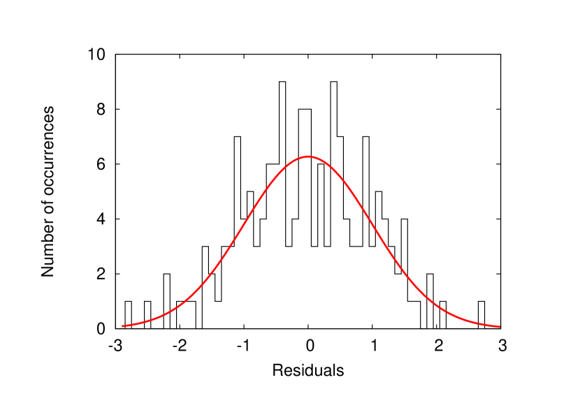
Figure 12: (Color online) Distribution of residuals normalized to their statistical error as obtained from a fit of the super-ratios by a function with nine free parameters. The red curve is the fit of the residuals by a normal distribution.

The solid black lines in Fig. 9 show the results from the fit. Figure 12 shows the residuals between the fit and the data points, normalized to their statistical error. Table 3 lists the values obtained for the fitted parameters and their associated uncertainties. The value of $\Delta$ obtained from the fit is $\Delta=-0.019(42)$ with a reduced $\chi^{2}$ of $\chi^{2}/\nu=1.17$.

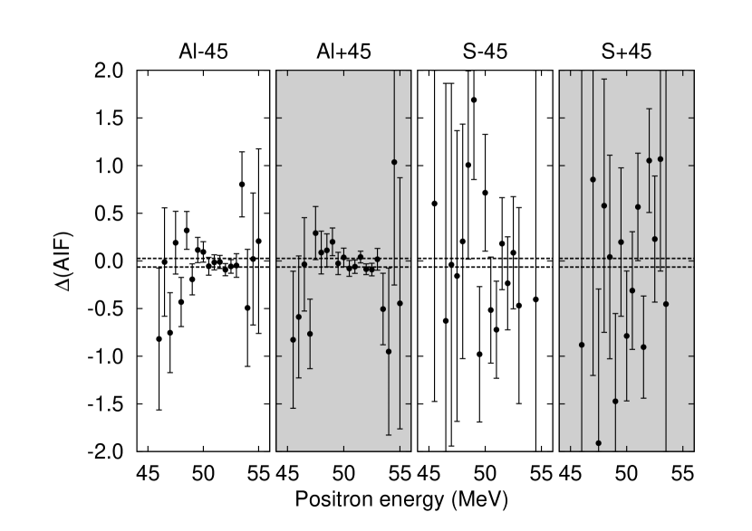
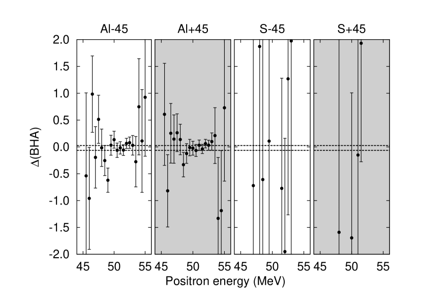
Figure 13: The values of $\Delta$ with their errors obtained after inversion of Eq. (23) for AIF events (upper panel) and BHA events (lower panel). The band delimited by the dotted lines indicate the $\pm 1\sigma$ interval of the fitted value of $\Delta$.

Equation (23) can be inverted and solved to express each value of $\Delta$ and its error as deduced from the value of the super-ratio. The result is shown in Fig. 13. The large reduction of uncertainty resulting from the larger enhancement factors near the maximal energies for the measurements with the polarization preserving Al targets is clearly visible. The loss of sensitivity for the data taken with the S target is also obvious. The data associated with AIF events have a larger sensitivity and dominate the precision on the final value of $\Delta$, but BHA scattering data also contribute.

Table 3: Results from the fit of the super ratios $s_{\beta}(x)$, using values of the muon polarization $P^{\mathrm{Al}}_{\mu}=0.937$ and $P^{\mathrm{S}}_{\mu}=0.382$.

Process	Target	$a_{\beta}$	$b_{\beta}$
AIF	Al	$\phantom{-}0.316(46)$	$\phantom{-}0.000(2)$
AIF	S	$\phantom{-}0.432(29)$	$\phantom{-}0.005(2)$
BHA	Al	$\phantom{-}0.239(46)$	$\phantom{-}0.004(2)$
BHA	S	$\phantom{-}0.118(33)$	$\phantom{-}0.005(2)$

IV.9 Residual muon polarization

The preliminary measurements described in Sec. III.2 indicated that the residual polarization of muons in the S powder target could be as low as $P^{\mathrm{S}}_{\mu}=0.10(5)$, as obtained from the Hanle signals. However, such a low value of the residual polarization is not consistent with the values obtained from the fits of the shape of the energy distributions as measured with the spectrometer (Fig. 5) during the main experiment nor with the total positron yield ratio between Al and S targets normalized to the telescopes. In addition, the values obtained for $P^{\mathrm{S}}_{\mu}$ from the fits of the energy distributions for AIF, BHA, and MIC events are also not statistically compatible between them although the $\chi^{2}$ distributions present rather flat minima.

We have adopted a conservative assumption by considering a sufficiently broad interval for the residual polarization in the S target, $P^{\mathrm{S}}_{\mu}=0.382(33)$, which is deduced from the fits of the energy distributions for all configurations. The impact of the values of the residual polarization in the S target is then considered as a common (energy independent) systematic effect. A similar procedure was applied to the positron energy distributions obtained with the Al target and resulted in a residual polarization $P^{\mathrm{Al}}_{\mu}=0.937(3)$.

Similar fits as the one described in Sec. IV.8 have been performed with the extreme values $P^{\mathrm{S}}_{\mu}=0.349$ and $P^{\mathrm{S}}_{\mu}=0.415$. The half difference between the central values of $\Delta$ obtained from those fits plus the half difference between the errors on $\Delta$ is then taken as an estimate of the systematic error associated with the actual residual polarization in the S target.

The uncertainty on the muon polarization in the Al target has a negligible effect on the final result.

IV.10 Result

Increasing the statistical error given in Sec. IV.8 above by $\sqrt{\chi^{2}/\nu}=1.08$ to account for the quality of the fit and including the systematic error due to the value of $P^{\mathrm{S}}_{\mu}$ as described above, results in

$$\Delta=(-19\pm 45_{\rm stat}\pm 3_{\rm syst})\times 10^{-3}\,.$$ (24)

The uncertainty is dominated by statistics and the size of the systematic error shows the sensitivity of the result to the determination of the muon polarization.

From the definition of $\Delta$, Eq. (3), and setting $\xi=\xi^{\prime}=1$ we get the value for $\xi^{\prime\prime}$:

$$\xi^{\prime\prime}=0.981\pm 0.045_{\rm stat}\pm 0.003_{\rm syst}\,.$$ (25)

This value is consistent with the SM expectation $\xi^{\prime\prime}_{SM}=1$ and represents an order of magnitude improvement (Fig. 14) on the relative error over the current value of $\xi^{\prime\prime}$ obtained under the same assumptions $\xi=\xi^{\prime}=1$ Burkard et al. (1985a, b).

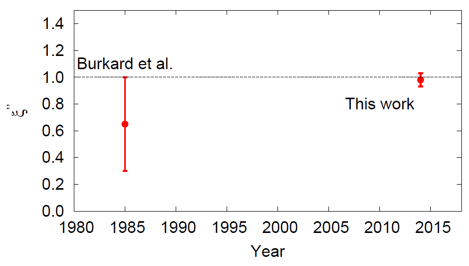
Figure 14: (color online) Measurements of the Michel Parameter $\xi^{\prime\prime}$ as a function of the year of publication.

V Implication on exotic couplings

The combination of Michel parameters contained in $\Delta$ can be expressed in terms of the effective couplings which appear in the interaction term, Eq. (1). The exact expression reads Fetscher and Gerber (1995)

$$\Delta=\frac{(a+4b+6c)(3a+4b-14c)}{(3a^{\prime}+4b^{\prime}-14c^{\prime})(a^{\prime}+4b^{\prime}+6c^{\prime})}-1$$ (26)

where $a$, $b$, $c$, $a^{\prime}$, $b^{\prime}$, and $c^{\prime}$ are bilinear functions of the couplings $g^{\gamma}_{\epsilon\mu}$ and are given in Refs. Fetscher and Gerber (1995); Beringer et al. (2012). Expanding to second order in the couplings which vanish in the SM, and setting $g^{V}_{LL}=1$, the expression in Eq. (26) becomes

$$\Delta\approx 8\left|g^{V}_{RL}\right|^{2}+4\left|g^{V}_{RR}\right|^{2}+\left|g^{S}_{RR}\right|^{2}+$$ (27)

$$+16\left|g^{T}_{RL}\right|^{2}+8{\rm Re}\left(g^{S}_{RL}g^{T*}_{RL}\right)\,.$$

Note that this quantity is sensitive to any exotic interaction which would couple to the electron component of right-handed chirality. This includes the scalar, vector and tensor interactions. The nature of the effective couplings to which this measurement is sensitive is then different than other Michel parameters Bueno et al. (2011); Hillairet et al. (2012) so that within the most general context of purely leptonic weak interactions this experiment is definitely complementary to those measuring the spectrum shape and the decay asymmetry.

A recent global analysis of muon decay data Hillairet et al. (2012) has provided new limits on several of the couplings entering the expression of $\Delta$ in Eq. (27). Considering the current 90% C.L. limits $|g^{V}_{RR}|<0.017$ and $|g^{S}_{RR}|<0.035$ Hillairet et al. (2012), we neglect here their contribution. Further, we assume that time reversal invariance holds for all interactions so that all couplings are taken to be real.

To illustrate the level of sensitivity on exotic couplings obtained from this measurement we select two scenarios, and provide two dimensional exclusions plots, with either $g^{S}_{RL}=0$ or $g^{V}_{RL}=0$. Figure 15 shows the 90% C.L. limits obtained on $g^{V}_{RL}$ and $g^{T}_{RL}$ from this experiment (solid green line) as compared to the current limits Hillairet et al. (2012) (dashed red lines). The region outside the ellipse is excluded by the present work and shows a significant reduction of the previously allowed parameter region. Figure 16 shows the 90% C.L. constraints obtained on $g^{T}_{RL}$ and $g^{S}_{RL}$ from this experiment (solid green line) as compared to the current limits Hillairet et al. (2012) (dashed red lines). The region outside the hyperbolas are excluded by the present work.

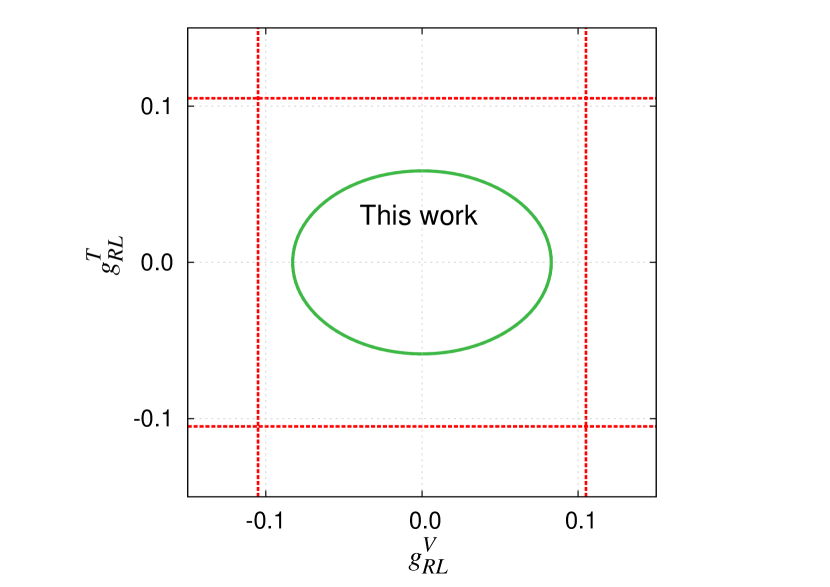
Figure 15: (Color online) Constraints at 90% C.L. on exotic couplings $g^{T}_{RL}$ and $g^{V}_{RL}$ obtained from the present experiment (solid green curve), assuming $g^{V}_{RR}=g^{S}_{RR}=g^{S}_{RL}=0$, and compared to the current limits (dashed red lines).

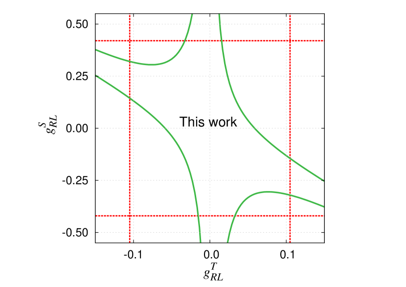
Figure 16: (Color online) Constraints at 90% C.L. on exotic couplings $g^{T}_{RL}$ and $g^{S}_{RL}$ obtained from the present experiment (solid green curve), assuming $g^{V}_{RR}=g^{S}_{RR}=g^{V}_{RL}=0$, and compared to the current limits (dashed red lines).

The result in Eq. (24) can also be interpreted within current specific scenarios extending the SM. A natural framework for the interpretation of parity-violating (i.e. pseudo-scalar) quantities is provided by left-right symmetric models Mohapatra and Pati (1975). Such models introduce charged right-handed bosons, $W^{\pm}_{R}$, that restore left-right symmetry by coupling to right-handed fermion doublets. The observation of parity violation at low energies is then attributed to the large mass, $m_{R}$, of the right-handed bosons relative to the standard left-handed one.

Several muon-decay parameters have been expressed in terms of parameters of general left-right symmetric models Herczeg (1986). For the combination of Michel parameters which enter $\Delta$ in Eq. (3) we have

$$\Delta=4v_{e}v_{\mu}r^{4}\left(\frac{\delta_{M}+t^{2}}{1+\delta_{M}t^{2}}\right)^{2}$$ (28)

where $v_{l}=\sum_{i}^{\prime}\left|U_{li}^{R}\right|^{2}/\sum_{i}^{\prime}\left|U_{li}^{L}\right|^{2}$ with $U_{li}^{L}$ ($U_{li}^{R}$) denoting the elements of the Pontecorvo-Maki-Nakagawa-Sakata matrix, coupling the charged left-(right)-handed lepton of flavour $l=e,\ \mu$ to the mass eigenstate neutrino $\nu_{i}$; $r=g_{R}/g_{L}$ is the ratio between the gauge couplings of the right-handed and left-handed bosons; $\delta_{M}=(m_{1}/m_{2})^{2}$, with $m_{1}$ ($m_{2}$) being the mass of the light (heavy) boson; and $t=\tan\zeta$, with $\zeta$ the mixing angle between the charged bosons $W_{1}$ and $W_{2}$. The prime on the summation symbols indicates the inclusion of neutrinos whose masses are sufficiently small that they couple to the decay process.

To illustrate the sensitivity level to the heavy boson mass $m_{2}$, we consider here the simple scenario of manifest left-right symmetry, which implies $v_{l}=r=1$. Furthermore, including the tight constraint on the mixing angle, $\zeta$, obtained from the unitarity condition of the Cabibbo-Kobayashi-Maskawa quark mixing matrix Hardy and Towner (2009), Eq. (28) reduces to

$$\Delta=4\left(\frac{m_{1}}{m_{2}}\right)^{4}$$ (29)

with $m_{1(2)}=m_{L(R)}$. Under the assumptions above we find

$$m_{R}>235{~{}~{}\rm GeV}/c^{2}$$ (30)

at 90% C.L. Such a mass scale is already excluded by other experiments in muon decay Bueno et al. (2011) as well as several direct and indirect searches Beringer et al. (2012). This is however not surprising since, after all, the relative precision on $\xi^{\prime\prime}$ obtained from this experiment is a moderate 5%.

Independent of the above, and within the general phenomenological description of the muon decay amplitude of Eq. (1), this experiment provides new model independent constraints on three of the exotic couplings which are neither accessible by recent high precision measurements of other muon decay parameters nor by experiments at high energy colliders. A new global analysis of muon decay experiments, including the present result and without making assumptions on specific couplings, would be valuable in order to quantify the impact of all available data on the couplings describing the leptonic weak interaction.

VI Summary

We have provided a detailed description of the experimental setup and of the analysis of a differential measurement of the longitudinal polarization of positrons emitted from the decay of polarized and depolarized muons. The longitudinal polarization was measured as a function of the positron energy near the maximum of the energy spectrum. This property is sensitive to the Michel parameter $\xi^{\prime\prime}$ which has previously been measured only once Burkard et al. (1985a, b).

The development work and the preparation for this experiment were carried out in 1995–2000 and the data presented here was accumulated during a single six week run which took place in 2001. From an early stage in the data analysis Morelle (2002) it was observed that the measured asymmetries for the two types of processes were smaller than the maximum possible amplitudes expected in the case the detected events were identified with full efficiency as pure annihilation in flight or as Bhabha scattering. Such smaller asymmetries, consistent with results from preliminary Monte-Carlo simulations that included misidentified events, had been observed in a preliminary test Van Hove (2000) performed in 1999. The experiment was designed in such a way that Monte-Carlo simulations are not absolutely necessary for the data analysis besides their utility in the description of the spectrometer transmission function.

Despite the reduced sensitivity, the result obtained in this measurement has improved the relative uncertainty of the Michel parameter $\xi^{\prime\prime}$ by an order of magnitude, providing new constraints of phenomenological couplings describing the leptonic weak interaction.

The uncertainty obtained from this measurement is dominated by the statistical error which, in part, is also determined by the sensitivity. It is conceivable that a future experiment could improve the identification of the scattering events using tracking techniques with detectors of lower mass. It is also possible to control the residual muon polarization such as to reduce the systematic error by at least a factor of 3, in order to reach a precision level of $10^{-3}$ in a future improved measurement.

References

- Herczeg (1986) P. Herczeg, Phys. Rev. D 34, 3449 (1986).
- Kuno and Okada (2001) Y. Kuno and Y. Okada, Rev. Mod. Phys. 73, 151 (2001).
- Fetscher et al. (1986) W. Fetscher, H.-J. Gerber, and K. F. Johnson, Phys. Lett. B 173, 102 (1986).
- Michel (1950) L. Michel, Proc. Phys. Soc. Sec. A 63, 514 (1950).
- Fetscher and Gerber (1995) W. Fetscher and H.-J. Gerber, in Precision Tests of the Standard Electroweak Model, edited by P. Langacker (World Scientific, Singapore, 1995), vol. 14 of Advanced series directions in high energy physics, p. 657.
- Beringer et al. (2012) J. Beringer, J. F. Arguin, R. M. Barnett, K. Copic, O. Dahl, D. E. Groom, C. J. Lin, J. Lys, H. Murayama, C. G. Wohl, et al. (Particle Data Group), Phys. Rev. D 86, 010001 (2012).
- Bueno et al. (2011) J. F. Bueno, R. Bayes, Y. I. Davydov, P. Depommier, W. Faszer, C. A. Gagliardi, A. Gaponenko, D. R. Gill, A. Grossheim, P. Gumplinger, et al. (TWIST Collaboration), Phys. Rev. D 84, 032005 (2011).
- Hillairet et al. (2012) A. Hillairet, R. Bayes, J. F. Bueno, Y. I. Davydov, P. Depommier, W. Faszer, C. A. Gagliardi, A. Gaponenko, D. R. Gill, A. Grossheim, et al. (TWIST Collaboration), Phys. Rev. D 85, 092013 (2012).
- Burkard et al. (1985a) H. Burkard, F. Corriveau, J. Egger, W. Fetscher, H.-J. Gerber, K. F. Johnson, H. Kaspar, H. J. Mahler, M. Salzmann, and F. Scheck, Phys. Lett. B 150, 242 (1985a).
- Burkard et al. (1985b) H. Burkard, F. Corriveau, J. Egger, W. Fetscher, H.-J. Gerber, K. F. Johnson, H. Kaspar, H. J. Mahler, M. Salzmann, and F. Scheck, Phys. Lett. B 160, 343 (1985b).
- Mehr and Scheck (1979) M. T. Mehr and F. Scheck, Nucl. Phys. B 149, 123 (1979), erratum: Nucl. Phys. B 234 547 (1984).
- Scheck (1978) F. Scheck, Phys. Rep. 44, 187 (1978).
- Possoz et al. (1979) A. Possoz, L. Grenacs, J. Lehmann, L. Palffy, J. Julien, and C. Samour, Phys. Lett. B 87, 35 (1979).
- Van Hove (2000) P. Van Hove, Ph.D. thesis, UCL Louvain–la–Neuve (2000), (unpublished).
- Foroughi (2000) F. Foroughi (2000), private communication.
- (16) CERN Program Library Long Writeup W5013 (1994).
- Bincer (1957) A. M. Bincer, Phys. Rev. 107, 1434 (1957).
- Ford and Mullin (1957) G. W. Ford and C. J. Mullin, Phys. Rev. 108, 477 (1957), errata: G. W. Ford and C. J. Mullin, Phys. Rev. 110, 1485 (1958).
- McMaster (1960) W. H. McMaster, Il Nuovo Cimento 17, 395 (1960).
- Page (1957) L. A. Page, Phys. Rev. 106, 394 (1957).
- Fetscher (2007) W. Fetscher, EPJ C 52, 1 (2007).
- Corriveau et al. (1981) F. Corriveau, J. Egger, W. Fetscher, H. J. Gerber, K. F. Johnson, H. J. Mahler, M. Salzmann, H. Kaspar, and F. Scheck, Phys. Rev. D 24, 2004 (1981).
- Vacuumschelze (2002) Vacuumschelze, in Soft Magnetic Materials and Semi-finished Products, Heat Treatment (Vacuumschmelze GMBH & Co, 2002), p. 15.
- Morelle (2002) X. Morelle, Ph.D. thesis, ETH-Zurich #14604 (2002), (unpublished).
- Danneberg et al. (2005) N. Danneberg, W. Fetscher, K.-U. Köhler, J. Lang, T. Schweizer, A. von Allmen, K. Bodek, L. Jarczyk, S. Kistryn, J. Smyrski, et al., Phys. Rev. Lett. 94, 021802 (2005).
- Barnett et al. (2000) I. C. Barnett, C. Bee, K. Bodek, A. Budzanowski, N. Danneberg, P. Eberhardt, W. Fetscher, C. Hilbes, M. Janousch, L. Jarczyk, et al., Nucl. Instrum. Methods in Phys. Res. A 455, 329 (2000).
- Mohapatra and Pati (1975) R. N. Mohapatra and J. C. Pati, Phys. Rev. D 11, 2558 (1975).
- Hardy and Towner (2009) J. C. Hardy and I. S. Towner, Phys. Rev. C 79, 055502 (2009).