In-Order Delivery Delay of Transport Layer Coding

Abstract

A large number of streaming applications use reliable transport protocols such as TCP to deliver content over the Internet. However, head-of-line blocking due to packet loss recovery can often result in unwanted behavior and poor application layer performance. Transport layer coding can help mitigate this issue by helping to recover from lost packets without waiting for retransmissions. We consider the use of an on-line network code that inserts coded packets at strategic locations within the underlying packet stream. If retransmissions are necessary, additional coding packets are transmitted to ensure the receiver’s ability to decode. An analysis of this scheme is provided that helps determine both the expected in-order packet delivery delay and its variance. Numerical results are then used to determine when and how many coded packets should be inserted into the packet stream, in addition to determining the trade-offs between reducing the in-order delay and the achievable rate. The analytical results are finally compared with experimental results to provide insight into how to minimize the delay of existing transport layer protocols.

I Introduction

Reliable transport protocols are used in a variety of settings to provide data transport for time sensitive applications. In fact, video streaming services such as Netflix and YouTube, which both use TCP, account for the majority of fixed and mobile traffic in both North America and Europe [1]. In fixed, wireline networks where the packet erasure rate is low, the quality of user experience (QoE) for these services is usually satisfactory. However, the growing trend towards wireless networks, especially at the network edge, is increasing non-congestion related packet erasures within the network. This can result in degraded TCP performance and unacceptable QoE for time sensitive applications. While TCP congestion control throttling is a major factor in the degraded performance, head-of-line blocking when recovering from packet losses is another. This paper will focus on the latter by applying coding techniques to overcome lost packets and reduce head-of-line blocking issues so that overall in-order packet delay is minimized.

These head-of-line blocking issues result from using techniques like selective repeat automatic-repeat-request (SR-ARQ), which is used in most reliable transport protocols (e.g., TCP). While it helps to ensure high efficiency, one problem with SR-ARQ is that packet recovery due to a loss can take on the order of a round-trip time ($RTT$) or more [2]. When the $RTT$ (or more precisely the bandwidth-delay product ($BDP$)) is very small and feedback is close to being instantaneous, SR-ARQ provides near optimal in-order packet delay. Unfortunately, feedback is often delayed and only contains a partial map of the receiver’s knowledge. This can have major implications for applications that require reliable delivery with constraints on the time between the transmission and in-order delivery of a packet. As a result, we are forced to look at alternatives to SR-ARQ.

This paper will explore the use of a systematic random linear network code (RLNC), in conjunction with a coded generalization of SR-ARQ, to help reduce the time needed to recover from losses. The scheme considered first adds redundancy to the original data stream by injecting coded packets at key locations to help overcome potential losses. This has the benefit of reducing the number of retransmissions and, consequently, the delay. However, correlated losses or incorrect information about the network can result in the receiver’s inability to decode. Therefore, feedback and coded retransmission of data is also considered.

The following sections will provide the answers to two questions about the proposed scheme: when should redundant packets be inserted into the original packet stream to minimize in-order packet delay; and how much redundancy should be added to meet a user’s requested QoE. These answers will be provided through an analysis of the in-order delivery delay as a function of the coding window size and redundancy. We will then use numerical results to help determine the cost (in terms of rate) of reducing the delay and as a tool to help determine the appropriate coding window size for a given network path/link. While an in-depth comparison of our scheme with others is not within the scope of this paper, we will use SR-ARQ as a baseline to help show the benefits of coding at the transport layer.

The remainder of the paper is organized as follows. Section II provides an overview of the related work in the area of transport layer coding and coding for reducing delay. Section III describes the coding algorithm and system model used throughout the paper. Section IV provides the tools needed to analyze the proposed scheme; and an analysis of the first two moments of the in-order delay are provided in Sections V and VI. Furthermore, the throughput efficiency is derived in Section VII to help determine the cost of coding. Numerical results are finally presented in Section VIII and we conclude in Section IX.

II Related Work

A resurgence of interest in coding at the transport layer has taken place to help overcome TCP’s poor performance in wireless networks. Sundararajan et. al. [3] first proposed TCP with Network Coding (TCP/NC). They insert a coding shim between the TCP and IP layers that introduces redundancy into the network in order to spoof TCP into believing the network is error-free. Loss-Tolerant TCP (LT-TCP) [4, 5, 6] is another approach using Reed-Solomon (RS) codes and explicit congestion notification (ECN) to overcome random packet erasures and improve performance. In addition, Coded TCP (CTCP) [7] uses RLNC [8] and a modified additive-increase, multiplicative decrease (AIMD) algorithm for maintaining high throughput in high packet erasure networks. While these proposals have shown coding can help increase throughput, especially in challenged networks, only anecdotal evidence has been provided showing the benefits for time sensitive applications.

On the other hand, a large body of research investigating the delay of coding in different settings has taken place. In general, most of these works can be summarized by Figure 1. The coding delay of chunked and overlapping chunked codes ([9]) (shown in Figure 1(a)), network coding in time-division duplexing (TDD) channels ([10, 11, 12]), and network coding in line networks where coding also occurs at intermediate nodes ([13]) is well understood. In addition, a non-asymptotic analysis of the delay distributions of random linear network coding (RLNC) ([14]) and various multicast scenarios ([15, 16, 17]) using a variant of the scheme in Figure 1(b) have also been investigated. Furthermore, the research that looks at the in-order packet delay is provided in [2] and [18] for uncoded systems, while [19], [20], and [21] considers the in-order packet delay for non-systematic coding schemes similar to the one shown in Figure 1(b). However, these non-systematic schemes may not be the optimum strategy in networks or communication channels with a long $RTT$.

Possibly the closest work to ours is that done by Joshi et. al. [22, 23] and Tömösközi et. al. [24]. Bounds on the expected in-order delay and a study of the rate/delay trade-offs using a time-invariant coding scheme is provided in [22] and [23] where they assume feedback is instantaneous, provided in a block-wise manner, or not available at all. A generalized example of their coding scheme is shown in Figure 1(c). While their analysis provides insight into the benefits of coding for streaming applications, their model is similar to a half-duplex communication channel where the sender transmits a finite block a information and then waits for the receiver to send feedback. Unfortunately, it is unclear if their analysis can be extended to full-duplex channels or models where feedback does not provide complete information about the receiver’s state-space. Finally, the work in [24] considers the in-order delay of online network coding where feedback determines the source packets used to generate coded packets. However, they only provide experimental results and do not attempt an analysis.

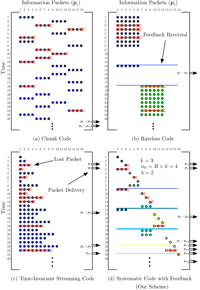
Figure 1: Coding matrices for various schemes assuming an identical loss pattern and a feedback delay of 4 time-slots. The columns represent the original information packet $\boldsymbol{p}_{i}$, and the rows represent the composition of the transmitted packet at time $t$ (e.g., the transmitted packet in time-slot 1 of (a) is $\boldsymbol{c}_{j}=\sum_{i=1}^{4}\alpha_{i,j}\boldsymbol{p}_{i}$ where $\alpha_{i,j}$ is defined in Section III). Lines within a matrix indicate when feedback about a generation (represented by different colors) was received.

III Coding Algorithm and System Model

We consider a time-slotted model to determine the coding window size $k$ and added redundancy $R\geq 1$ that minimizes the per-packet, or playback, delay $D$. The duration of each slot is $t_{s}=\nicefrac{{s_{pkt}}}{{Rate}}$ where $s_{pkt}$ is the size of each transmitted packet and $Rate$ is the transmission rate of the network. Also let $t_{p}$ be the propagation delay between the sender and the receiver (i.e., $RTT=t_{s}+2t_{p}$ assuming that the size of each acknowledgement is sufficiently small). Packet erasures are assumed to be independently and identically distributed (i.i.d.) with $\epsilon$ being the probability of a packet erasure within the network.

Source packets $\boldsymbol{p}_{i}$, $i=\{1,\ldots,N\}$, are first partitioned into coding generations $\boldsymbol{G}_{j}=\left\{\boldsymbol{p}_{\left(j-1\right)k+1},\ldots,\boldsymbol{p}_{\min\left(jk,N\right)}\right\}$, $j\in\left[1,\lceil\nicefrac{{N}}{{k}}\rceil\right]$. Each generation $\boldsymbol{G}_{j}$ is transmitted using the systematic network coding scheme shown in Algorithm 1 where the coding window spans the entire generation. The coded packets $\boldsymbol{c}_{j,m}$ shown in the algorithm are generated by taking random linear combinations of the $k$ information packets contained within the generation where the coding coefficients $\alpha_{i,j,m}\in\mathbb{F}_{q}$ are chosen at random and $\boldsymbol{p}_{i}$ is treated as a vector in $\mathbb{F}_{q}$. Once every packet in $\boldsymbol{G}_{j}$ has been transmitted (both uncoded and coded), the coding window slides to the next generation $\boldsymbol{G}_{j+1}$ and the process repeats without waiting for feedback.

1:  for all $j\in\left[1,\lceil\nicefrac{{N}}{{k}}\rceil\right]$ do

2:     for all Packets $\boldsymbol{p}_{i}$, $i\in\left[\left(j-1\right)k+1,\min\left(jk,N\right)\right]$ do

3:        Transmit $\boldsymbol{p}_{i}$

4:     for all $m\in\left[1,n_{k}-k\right]$ do

5:        Transmit $\boldsymbol{c}_{j,m}=\sum_{i=\left(j-1\right)k+1}^{\min\left(jk,N\right)}\alpha_{i,j,m}\boldsymbol{p}_{i}$

Algorithm 1 Code Generation Algorithm

We assume that delayed feedback is provided about each generation (i.e., multiple coding generations can be in-flight at any time); and this feedback contains the number of degrees of freedom ($dofs$) $l$ still required to decode the generation. If $l>0$, an additional $n_{l}=R\times l\geq l$ coded packets (or $dofs$) are retransmitted. This process is shown in Algorithm 2 and continues until all $k$ $dofs$ have been received and the generation can be decoded and delivered.

1:  $ACK$ From $G_{j}$ Received

2:  if No packets from $G_{j}$ in-flight and $l>0$ then

3:     for all $m\in\left[1,R\times l\right]$ do

4:        Transmit $\boldsymbol{c}_{j,m}=\sum_{i=\left(j-1\right)k+1}^{\min\left(jk,N\right)}\alpha_{i,j,m}\boldsymbol{p}_{i}$

Algorithm 2 $DOF$ Retransmission Algorithm

Figure 1(d) provides an example of the proposed scheme. Here we can see that source packets are partitioned into coding generations of size $k=3$ packets, and one coded packet is also transmitted for each generation (i.e., $R=1.33$). In this case, the first two packets of the blue generation can be delivered, but the third packet cannot since it is lost and the generation cannot be decoded. Delayed feedback indicates that additional $dofs$ are needed and two additional transmission attempts are required to successfully transmit the required $dof$. Once the $dof$ is delivered, the remainder of the blue generation, as well as the entire green generation, can be delivered in-order.

Due to the complexity of the process, several assumptions are needed. First, retransmissions occur immediately after feedback is obtained indicating additional $dofs$ are needed without waiting for the coding window to shift to a new generation. Second, the time to transmit packets after the first round does not increase the delay. For example, the packet transmission time is $t_{s}$ seconds. Assuming $l$ $dof$ retransmissions are needed, the additional $n_{l}t_{s}$ seconds needed to transmit these packets are not taken into account. Third, the number of previously transmitted generations that can cause head-of-line blocking is limited to $b-1$ where $b=\lceil\nicefrac{{BDP}}{{n_{k}}}\rceil$. Fourth, all packets within a generation are available to the transport layer without delay (i.e., we assume an infinite packet source). Finally, the coding window/generation size with the added redundancy is smaller than the $BDP$ (i.e., $n_{k}<BDP$). Without this assumption, feedback will be received prior to the transmission of the coded packets allowing for the use of SR-ARQ without a large impact to the performance.

It is important to note that these assumptions provide a lower bound. The first two assumptions ensure feedback is acted upon immediately and does not impact the delay experienced by other generations. The third assumption limits the possibility of a previously transmitted generation preventing delivery, thereby decreasing the overall delay.

IV Preliminaries

We first define several probability distributions and random variables that will be used extensively in later sections. Define $\left[P\right]\in\mathbb{R}^{k+1\times k+1}$ to be the transition matrix of a Markov chain. Each transition within the chain represents the number of $dofs$, or packets, successfully received after a round of transmissions, and each state represents the number of $dofs$ still needed by the client to decode. As a result, the elements of $\left[P\right]$ can be defined as follows:

$$\left[P_{ij}\right]=\begin{cases}B\left(n_{i},i-j,1-\epsilon\right)&\text{for }i\in[1,k],0<j\leq i\\ \sum_{m=i}^{n_{i}}B\left(n_{i},m,1-\epsilon\right)&\text{for }i\in[1,k],j=0\\ 1&\text{for }i=0,j=0,\end{cases}$$ (1)

where $B(n,k,p)={n\choose k}p^{k}(1-p)^{n-k}$. Let $X_{r}$ be the state of the chain at time $r$. It follows that $\text{Pr}\{X_{r}=j|X_{0}=i\}=\left[P_{ij}^{r}\right]$ for $r\geq 1$ and $\left[P_{ij}^{0}\right]=0$. In our model, $X_{0}=k$ with probability equal to 1 and a generation is successfully decoded when state $0$ is entered at time $r\geq 1$. Furthermore, the probability $\left[P_{i0}^{r}\right]$ is the probability that all packets within a single generation have been successfully received in or before $r$ transmission rounds.

Using this Markov chain, define $Y$ to be the number of transmission rounds required to transfer a single generation. The distribution on $Y$ is:

$$p_{Y}(y)=\begin{cases}\left[P_{k0}^{y}\right]-\left[P_{k0}^{y-1}\right]&\text{for }y\geq 1\\ 0&\text{otherwise.}\end{cases}$$ (2)

Next, define $Z_{i}$ to be the number of transmission rounds required to transfer $i$ generations. Before defining the distribution on $Z_{i}$, we first provide the following Lemma.

Lemma 1.

Let $N$ independent processes defined by the transition matrix $\left[P\right]$ start at the same time. The probability that all processes complete in less than or equal to $z$ rounds, or transitions, with at least one process completing in round $z$ is $\text{Pr}\{Z=z\}=\left[P_{k0}^{z}\right]^{N}-\left[P_{k0}^{z-1}\right]^{N}$.

Proof:

Let $f\left(z\right)=1-\sum_{j=1}^{z-1}p_{Y}\left(j\right)$. The probability of $N$ independent processes completing in less than or equal to $z$ rounds with at least one process completing in round $z$ is:

$$\text{Pr}\{Z=z\} =\sum_{i=1}^{N}B\left(N,i,f\left(z\right)\right)\left(\frac{p_{Y}\left(z\right)}{f\left(z\right)}\right)^{i}$$ (3)

$$=\sum_{i=1}^{N}{N\choose i}\left(p_{Y}\left(z\right)\right)^{i}\left[P_{k0}^{z-1}\right]^{N-i}$$ (4)

$$=\frac{\left[P_{k0}^{z-1}\right]^{N+1}\left(\left[P_{k0}^{z}\right]^{N+1}-\left[P_{k0}^{z-1}\right]^{N+1}\right)}{\left[P_{k0}^{z-1}\right]^{N+1}\left[P_{k0}^{z}\right]}$$

$$-\frac{\left[P_{k0}^{z-1}\right]^{2N+1}\left(\left[P_{k0}^{z}\right]-\left[P_{k0}^{z-1}\right]\right)}{\left[P_{k0}^{z-1}\right]^{N+1}\left[P_{k0}^{z}\right]}$$ (5)

$$=\left[P_{k0}^{z}\right]^{N}-\left[P_{k0}^{z-1}\right]^{N}.$$ (6)

∎

Given Lemma 1, the distribution on $Z_{i}$ is:

$$p_{Z_{i}}(z_{i})=\begin{cases}\left[P_{k0}^{z_{i}}\right]^{i}-\left[P_{k0}^{z_{i}-1}\right]^{i}&\text{for }z_{i}\geq 1,i\leq b-1\\ 0&\text{otherwise.}\end{cases}$$ (7)

Also define $S$ to be the number of uncoded packets that are successfully transferred within a generation prior to the first packet loss. The distribution on $S$ is:

$$p_{S|Y}(s|y)=\begin{cases}\epsilon\left(1-\epsilon\right)^{s}&\text{for }s\in[0,k-1],y=1\\ \left(1-\epsilon\right)^{s}&\text{for }s=k,y=1\\ \frac{\epsilon\left(1-\epsilon\right)^{s}}{1-\left(1-\epsilon\right)^{k}}&\text{for }s\in[0,k-1],y\neq 1,\\ 0&\text{otherwise},\end{cases}$$ (8)

and its first three moments are given by the following lemma.

Lemma 2.

Define $\overline{s_{1}^{i}}=\mathbb{E}\left[S^{i}|Y=1\right]$ and $\overline{s_{2}^{i}}=\mathbb{E}\left[S^{i}|Y\neq 1\right]$. Then given $Y=y$, the first through third moments of $S$ are

$$\overline{s_{1}^{1}} =\frac{1-\epsilon}{\epsilon}\left(1-\left(1-\epsilon\right)^{k}\right),$$ (9)

$$\overline{s_{1}^{2}} =\frac{2\left(1-\epsilon\right)}{\epsilon^{2}}\left(1-\left(k\epsilon+1\right)\left(1-\epsilon\right)^{k}\right)-\overline{s_{1}^{1}},$$ (10)

$$\overline{s_{1}^{3}} =\frac{6\left(1-\epsilon\right)^{3}}{\epsilon^{3}}\left(1-\left(k\epsilon+1\right)(1-\epsilon)^{k}\right)+3\left(1-\epsilon\right)\overline{s_{1}^{2}}$$

$$-\frac{3k}{\epsilon}\left(k+1\right)\left(1-\epsilon\right)^{k+1}+\left(4-3\epsilon\right)\overline{s_{1}^{1}},$$ (11)

and

$$\overline{s_{2}^{i}}=\frac{\overline{s_{1}^{i}}-k^{i}\left(1-\epsilon\right)^{k}}{1-\left(1-\epsilon\right)^{k}},$$ (12)

for $i=1,2,3$.

Proof:

Define the moment generating function of $S$ when $Y=1$ to be

$$M_{S|Y}(t) = \mathbb{E}[e^{tS}|Y=1]$$ (13)

$$= \frac{\epsilon\left(1-e^{kt}\left(1-\epsilon\right)^{k}\right)}{1-e^{t}+\epsilon e^{t}}+e^{kt}\left(1-\epsilon\right)^{k}.$$ (14)

The first, second, and third moments of $S$ when $Y=1$ are then $\nicefrac{{\delta}}{{\delta t}}M_{S|Y}(0)$, $\nicefrac{{\delta^{2}}}{{\delta t^{2}}}M_{S|Y}(0)$, and $\nicefrac{{\delta^{3}}}{{\delta t^{3}}}M_{S|Y}(0)$ respectively.

For $Y\neq 1$, we need to scale the above expectations accordingly. This can be done by subtracting the term $k^{i}\left(1-\epsilon\right)^{k}$ from each of the moments above and dividing by $1-\left(1-\epsilon\right)^{k}$. ∎

Finally, let $V_{i}$, $i\leq b-1$, describe the position of the last received generation preventing delivery in round $z_{i}$. The following lemma helps to define the distribution on $V_{i}$.

Lemma 3.

Let $N$ independent processes defined by the transition matrix $\left[P\right]$ start at the same time, and all processes complete in or before round $z_{N}$ with at least one process completing in round $z_{N}$. The probability that the $j$th process is the last to complete is defined by the distribution

$$p_{V_{N}|Z_{N}}\left(v_{N}|z_{N}\right)=\frac{\left[P_{k0}^{z_{N}}\right]^{N-v_{N}-1}\left[P_{k0}^{z_{N}-1}\right]^{v_{N}}p_{Y}\left(z_{N}\right)}{p_{Z_{N}}(z_{N})}$$ (15)

for $v_{N}=0,\ldots N-1$, $j=N-v_{N}$, $p_{Y}(y)$ defined in (2), and $p_{Z_{i}}\left(z_{i}\right)$ defined in (7). Furthermore, define $\overline{v_{N}^{i}}=\mathbb{E}\left[V_{N}^{i}|Z_{N}\right]$. Then

$$\overline{v_{N}^{1}}=\frac{\left[P_{k0}^{z_{N}-1}\right]}{p_{Y}\left(z_{N}\right)}-\frac{N\left[P_{k0}^{z_{N}-1}\right]^{N}}{p_{Z_{N}}\left(z_{N}\right)},$$ (16)

and

$$\overline{v_{N}^{2}} = \frac{\left[P_{k0}^{z_{N}-1}\right]}{p_{Y}\left(z_{N}\right)}+\frac{2\left[P_{k0}^{z_{N}-1}\right]^{2}}{p_{Y}^{2}\left(z_{N}\right)}-\frac{N^{2}\left[P_{k0}^{z_{N}-1}\right]^{N}}{p_{Z_{N}}\left(z_{N}\right)}$$ (17)

$$-\frac{2N\left[P_{k0}^{z_{N}-1}\right]^{N+1}}{p_{Y}\left(z_{N}\right)p_{Z_{N}}\left(z_{N}\right)}.$$

Proof:

Let $\beta_{z_{N}}=\nicefrac{{p_{Y}\left(z_{N}\right)}}{{\left[P_{k0}^{z_{N}}\right]}}$, be the probability of a generation finishing in round $z_{N}$ given all of the $N$ generations have completed transmission in or before round $z_{N}$. The distribution on $V_{N}\in[0,N-1]$ is

$$p_{V_{N}|Z_{N}}\left(v_{N}|z_{N}\right) =\frac{\beta_{z_{N}}\left(1-\beta_{z_{N}}\right)^{v_{N}}}{\sum_{j=0}^{N-1}\beta_{z_{N}}\left(1-\beta_{z_{N}}\right)^{j}}$$ (18)

$$=\frac{\beta_{z_{N}}\left(1-\beta_{z_{N}}\right)^{v_{N}+1}}{1-\left(1-\beta_{z_{N}}\right)^{N}}$$ (19)

$$=\frac{\left[P_{k0}^{z_{N}}\right]^{N-v_{N}-1}\left[P_{k0}^{z_{N}-1}\right]^{v_{N}}p_{Y}\left(z_{N}\right)}{p_{Z_{N}}(z_{N})}.$$ (20)

Define the moment generating function of $V_{N}$ given $Z_{N}$ to be

$$M_{V_{N}|Z_{N}}(t) =\mathbb{E}[e^{tV_{N}}|Z_{N}=z_{N}]$$

$$=\frac{\left(\left[P_{k0}^{z_{N}}\right]^{N}-\left[P_{k0}^{z_{N}-1}\right]^{N}e^{Nt}\right)p_{Y}(z_{N})}{\left(\left[P_{k0}^{z_{N}}\right]-\left[P_{k0}^{z_{N}-1}\right]e^{t}\right)p_{Z_{N}}(z_{N})}.$$ (21)

The first and second moments of $V_{N}$ given $Z_{N}$ are $\nicefrac{{\delta}}{{\delta t}}M_{V_{N}|Z_{N}}(0)$ and $\nicefrac{{\delta^{2}}}{{\delta t^{2}}}M_{V_{N}|Z_{N}}(0)$ respectively. ∎

Now that we have the distributions for the random variables $Y$, $Z_{i}$, $S$, and $V_{i}$, as well as several relevant moments, we have the tools needed to derive the expected in-order delivery delay.

V Expected In-Order Delivery Delay

A lower bound on the expected delay, $\mathbb{E}[D]$, can be derived using the law of total expectation:

$$\mathbb{E}[D] = \mathbb{E}_{Y}\left[\mathbb{E}_{Z_{b-1}}\left[\mathbb{E}_{D}\left[D|Y,Z_{b-1}\right]\right]\right].$$ (22)

From (22), there are four distinct cases that must be evaluated. For each case, define $\bar{d}_{Y=y,Z=z}=\mathbb{E}\left[D|Y=y,Z_{b-1}=z\right]$.

V-A Case 1: $Y=1,Z_{b-1}=1$

The latest generation in transit completes within the first round of transmission and no previously transmitted generations prevent delivery. As a result, all packets received prior to the first loss (i.e., packets $\boldsymbol{p}_{1},\ldots\boldsymbol{p}_{s}$) are immediately delivered. Once a packet loss is observed, packets received after the loss (i.e., packets $\boldsymbol{p}_{s+1},\ldots,\boldsymbol{p}_{k}$) are buffered until the entire generation is decoded. An example is given in Figure 2(a) where $n_{k}=6$, $k=4$, the number of packets received prior to the first loss is $s=2$, and the number of coded packets needed to recover from the two packet losses is $c=2$. Taking the expectation over all $S$ and all packets within the generation, the mean delay is

$$\bar{d}_{Y=1,Z=1} =\sum_{s=0}^{k-1}\left(\left(t_{s}+t_{p}\right)\frac{s}{k}+\frac{1}{k}\sum_{i=0}^{k-s-1}\biggl{(}t_{p}+\bigl{(}k-s-i\right.$$

$$+\mathbb{E}\left[C|S\right]\bigr{)}t_{s}\biggr{)}\Biggr{)}p_{S|Y}\left(s|1\right)+\left(t_{s}+t_{p}\right)p_{S|Y}\left(k|1\right)$$ (23)

$$=t_{p}+\frac{t_{s}}{2k}\biggl{(}\overline{s_{1}^{2}}-\left(2k-1\right)\overline{s_{1}^{1}}+k\left(k+1\right)$$

$$+2\sum_{s=0}^{k-1}\left(k-s\right)\mathbb{E}\left[C|S\right]p_{S|Y}\left(s|1\right)\biggr{)}$$ (24)

$$\geq t_{p}+\frac{t_{s}}{2k}\biggl{(}\overline{s_{1}^{2}}-\left(2k-1\right)\overline{s_{1}^{1}}+k\left(k+1\right)$$

$$+2\sum_{s=0}^{k-1}\left(k-s\right)p_{S|Y}\left(s|1\right)\biggr{)}$$ (25)

$$=\frac{t_{s}}{2k}\biggl{(}\overline{s_{1}^{2}}-\left(2k+1\right)\overline{s_{1}^{1}}+k\left(k+3\right)\biggr{)}+t_{p},$$ (26)

where $\overline{s_{1}^{1}}$ and $\overline{s_{1}^{2}}$ are given by Lemma 2; and $\mathbb{E}\left[C|S\right]$ is the expected number of coded packets needed to recover from all packet erasures occurring in the first $k$ packets. When $s<k$, the number of coded packets required is at least one (i.e., $\mathbb{E}\left[C|S\right]\geq 1$) leading to the bound in (25).

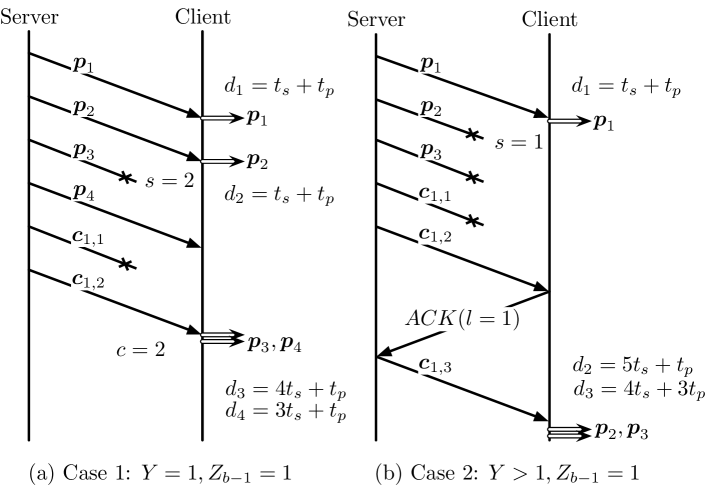
Figure 2: Example of (a) case 1 and (b) case 2. The delay $d_{i}$ of each packet is listed next to the time when it is delivered to the application layer.

V-B Case 2: $Y>1,Z_{b-1}=1$

All packets $\left\{\boldsymbol{p}_{1},\ldots\boldsymbol{p}_{s}\right\}$ are delivered immediately until the first packet loss is observed. Since $Y>1$, at least one retransmission event is needed to properly decode. Once all $k$ $dofs$ have been received and the generation can be decoded, the remaining packets $\left\{\boldsymbol{p}_{s+1},\ldots,\boldsymbol{p}_{k}\right\}$ are delivered in-order. An example is provided in Figure 2(b). The generation cannot be decoded because there are too many packet losses during the first transmission attempt. As a result, one additional $dof$ is retransmitted allowing the client to decode in round two (i.e., $Y=2$). Taking the expectation over all $S$ and all packets within the generation, the expected delay for this case is

$$\bar{d}_{Y>1,Z=1} =\frac{1}{k}\sum_{s=0}^{k-1}\biggl{(}\left(t_{p}+t_{s}\right)s+\sum_{i=0}^{k-s-1}\Bigl{(}t_{p}+2\left(y-1\right)t_{p}$$

$$+\left(k-s-i+n_{k}-k\right)t_{s}\Bigr{)}\biggr{)}p_{S|Y}(s|y\neq 1)$$ (27)

$$=\biggl{(}\frac{1}{2k}\overline{s_{2}^{2}}-\frac{1}{2k}\left(2n_{k}-1\right)\overline{s_{2}^{1}}+n_{k}-\frac{1}{2}k+\frac{1}{2}\biggr{)}t_{s}$$

$$-\biggl{(}\frac{2}{k}\left(y-1\right)\overline{s_{2}^{1}}-2y+1\biggr{)}t_{p},$$ (28)

where $\overline{s_{2}^{1}}$ and $\overline{s_{2}^{2}}$ are given by Lemma 2. It is important to note that we do not take into account the time to transmit packets after the first round (see the assumptions in Section III).

V-C Case 3: $Z_{b-1}>Y\geq 1,Z_{b-1}>1$

In this case, generation $\boldsymbol{G}_{j}$ completes prior to a previously sent generation. As a result, all packets $\left\{\boldsymbol{p}_{\left(j-1\right)k+1},\dots,\boldsymbol{p}_{jk}\right\}\in\boldsymbol{G}_{j}$ are buffered until all previous generations have been delivered. Once there are no earlier generations preventing in-order delivery, all packets in $\boldsymbol{G}_{j}$ are immediately delivered. Figure 3(a) provides an example. Consider the delay experienced by packets in $\boldsymbol{G}_{3}$. While $\boldsymbol{G}_{3}$ is successfully decoded after the first transmission attempt, generation $\boldsymbol{G}_{1}$ cannot be decoded forcing all packets in $\boldsymbol{G}_{3}$ to be buffered until $\boldsymbol{G}_{1}$ is delivered. Taking the expectation over all packets within the generation and all possible locations of the last unsuccessfully decoded generation, the expected delay is

$$\bar{d}_{Z>Y\geq 1,Z>1} =\frac{1}{k}\sum_{i=1}^{k}\biggl{(}\left(n_{k}-k+i\right)t_{s}+t_{p}+2t_{p}\left(z-1\right)$$

$$-\left(\overline{v_{b-1}^{1}}+1\right)n_{k}t_{s}\biggr{)}$$ (29)

$$=\left(2z-1\right)t_{p}-\left(\overline{v_{b-1}^{1}}n_{k}+\frac{k-1}{2}\right)t_{s},$$ (30)

where $\overline{v_{b-1}^{1}}$ is given by Lemma 3.

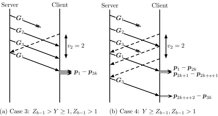
Figure 3: Example of (a) case 3 and (b) case 4 where $b=3$.

V-D Case 4: $Y\geq Z_{b-1},Z_{b-1}>1$

Finally, this case is a mixture of the last two. The generation $\boldsymbol{G}_{j}$ completes after all previously transmitted generations, but it requires more than one transmission round to decode. Packets received before the first packet loss are buffered until all previous generations are delivered, and packets received after the first packet loss are buffered until $\boldsymbol{G}_{j}$ can be decoded. An example is provided in Figure 3(b). Consider the delay of packets in $\boldsymbol{G}_{3}$. Both $\boldsymbol{G}_{1}$ and $\boldsymbol{G}_{3}$ cannot be decoded after the first transmission attempt. After the second transmission attempt, $\boldsymbol{G}_{1}$ can be decoded allowing packets $\left\{\boldsymbol{p}_{2k+1},\ldots,\boldsymbol{p}_{2k+s+1}\right\}\in\boldsymbol{G}_{3}$ to be delivered; although packets $\left\{\boldsymbol{p}_{2k+s+2},\ldots,\boldsymbol{p}_{3k}\right\}\in\boldsymbol{G}_{3}$ must wait to be delivered until after $\boldsymbol{G}_{3}$ is decoded. Taking the expectation over all $S$, all packets within the generation, and all possible locations of the last unsuccessfully decoded generation, the expected delay is

$$\bar{d}_{Y\geq Z,Z>1} =\frac{1}{k}\sum_{s=0}^{k-1}\Biggl{(}\sum_{i=1}^{s}\biggl{(}\left(n_{k}-i+1\right)t_{s}+2t_{p}\left(z-\frac{1}{2}\right)$$

$$-\left(\overline{v_{b-1}^{1}}+1\right)n_{k}t_{s}\biggr{)}+\sum_{j=s+1}^{k}\Bigl{(}2t_{p}\Bigl{(}y-\frac{1}{2}\Bigr{)}$$

$$+\left(n_{k}-j+1\right)t_{s}\Bigr{)}\Biggr{)}p_{S|Y}(s|y\neq 1)$$ (31)

$$=\biggl{(}\frac{2\left(z-y\right)}{k}\overline{s_{2}^{1}}+2y-1\biggr{)}t_{p}$$

$$-\biggl{(}\frac{n_{k}}{k}\left(\overline{v_{b-1}^{1}}+1\right)\overline{s_{2}^{1}}-n_{k}+\frac{1}{2}k-\frac{1}{2}\biggr{)}t_{s}.$$ (32)

The expectations $\overline{s_{2}^{1}}$ and $\overline{v_{b-1}^{1}}$ are given by Lemmas 2 and 16 respectively.

Combining the cases above, we obtain the following:

Theorem 4.

The expected in-order packet delay for the proposed coding scheme is lower bounded by

$$\mathbb{E}[D]\geq\sum_{z_{b-1}\geq 1}\sum_{y\geq 1}\bar{d}_{Y=y,Z=z_{b-1}}p_{Y}(y)p_{Z_{b-1}}(z_{b-1}).$$ (33)

where $\bar{d}_{Y=y,Z=z_{b-1}}$ is given in equations (26), (28), (30), and (32); and the distributions $p_{Y}(y)$ and $p_{Z_{b-1}}(z_{b-1})$ are given in equations (2) and (7) respectively.

VI In-Order Delivery Delay Variance

The second moment of the in-order delivery delay can be determined in a similar manner as the first. Again, we can use the law of total expectation to find the moment:

$$\mathbb{E}[D^{2}] = \mathbb{E}_{Y}\left[\mathbb{E}_{Z_{b-1}}\left[\mathbb{E}_{D}\left[D^{2}|Y,Z_{b-1}\right]\right]\right].$$ (34)

As with the first moment, four distinct cases exist that must be dealt with separately. For each case, define $\bar{d}_{Y=y,Z=z}^{2}=\mathbb{E}\left[D^{2}|Y=y,Z_{b-1}=z\right]$. While we omit the initial step in the derivation of each case, $\bar{d}_{Y,Z}^{2}$ can be determined using the same assumptions as above.

VI-A Case 1: $Y=1,Z_{b-1}=1$

Using the expectations defined in Lemma 2, the second moment $\bar{d}_{Y=1,Z=1}^{2}$ is shown below. For $s<k$, the number of coded packets needed to decode the generation will always be greater than or equal to one (i.e., $c\geq 1$). Therefore, the bound in (35) follows from letting $c=1$ and $p_{C|S}\left(1|s\right)=1$ for all $s$.

$$\bar{d}_{Y=1,Z=1}^{2} \geq t_{p}^{2}+\left(k+3\right)t_{p}t_{s}+\frac{1}{6}\left(2k^{2}+9k+13\right)t_{s}^{2}$$

$$-\biggl{(}\left(k+3+\frac{7}{6k}\right)t_{s}^{2}+\left(\frac{2k+1}{k}\right)t_{p}t_{s}\biggr{)}\overline{s_{1}^{1}}$$

$$+\Biggl{(}\left(\frac{2k+3}{2k}\right)t_{s}^{2}+\frac{1}{k}t_{p}t_{s}\Biggr{)}\overline{s_{1}^{2}}-\frac{1}{3k}t_{s}^{2}\overline{s_{1}^{3}}.$$ (35)

VI-B Case 2: $Y>1,Z_{b-1}=1$

This case can be derived in a similar manner as the last. Again, each $\overline{s_{2}^{i}}$, $i=\left\{1,2,3\right\}$, are given by Lemma 2.

$$\bar{d}_{Y>1,Z=1}^{2}$$

$$= \biggl{(}n_{k}\left(n_{k}-k+1\right)+\frac{1}{6k}\left(2k^{3}-3k^{2}+k+6\right)\biggr{)}t_{s}^{2}$$

$$+ \biggl{(}2n_{k}\left(2y-1\right)-2y\left(k-1\right)+k-1+\frac{2}{k}\biggr{)}t_{p}t_{s}$$

$$+ \frac{1}{2k}\left(\left(2n_{k}+1\right)t_{s}^{2}+2\left(2y-1\right)t_{p}t_{s}\right)\overline{s_{2}^{2}}-\frac{1}{3k}t_{s}^{2}\overline{s_{2}^{3}}$$

$$- \frac{1}{k}\biggl{(}(n_{k}^{2}+n_{k}+\frac{1}{6})t_{s}^{2}+\left(2y-1\right)\left(2n_{k}+1\right)t_{p}t_{s}$$

$$+ (2y-1)^{2}t_{p}^{2}\biggr{)}\overline{s_{2}^{1}}+\left(\left(2y-1\right)^{2}+\frac{1}{k}\right)t_{p}^{2}.$$ (36)

VI-C Case 3: $Z_{b-1}>Y\geq 1,Z_{b-1}>1$

The second moment $\bar{d}_{Z>Y\geq 1,Z>1}^{2}$ can be derived as follows:

$$\bar{d}_{Z>Y\geq 1,Z>1}^{2}$$

$$= \biggl{(}n_{k}^{2}\overline{v_{b-1}^{2}}+\left(k-1\right)\left(n_{k}\overline{v_{b-1}^{1}}+\frac{1}{3}k-\frac{1}{6}\right)\biggr{)}t_{s}^{2}$$

$$- (2z-1)\biggl{(}2n_{k}\overline{v_{b-1}^{1}}+k-1\biggr{)}t_{p}t_{s}+(2z-1)^{2}t_{p}^{2}.$$ (37)

VI-D Case 4: $Y\geq Z_{b-1},Z_{b-1}>1$

Using Lemmas 2 and 3, the second moment $\bar{d}_{Y\geq Z,Z>1}^{2}$ is:

$$\bar{d}_{Y\geq Z,Z>1}^{2}$$

$$= \left(2y-1\right)\biggl{(}\left(2n_{k}-k+1\right)t_{s}t_{p}+\left(2y-1\right)t_{p}^{2}\biggr{)}$$

$$+ \biggl{(}n_{k}\left(n_{k}-k+1\right)+\frac{1}{6}\left(2k^{2}-3k+1\right)\biggr{)}t_{s}^{2}$$

$$+ \frac{1}{k}\biggl{(}n_{k}\left(\overline{v_{b-1}^{1}}+1\right)t_{s}^{2}+2\left(y-z\right)t_{p}t_{s}\biggr{)}\overline{s_{2}^{2}}$$

$$+ \frac{1}{k}\biggl{(}n_{k}\Bigl{(}n_{k}\left(\overline{v_{b-1}^{2}}-1\right)-\overline{v_{b-1}^{1}}-1\Bigr{)}t_{s}^{2}$$

$$- 2\biggl{(}n_{k}\left(\overline{v_{b-1}^{1}}\left(2z-1\right)+\left(2y-1\right)\right)+y-z\biggr{)}t_{p}t_{s}$$

$$- 4\left(y-z\right)\left(y+z-1\right)t_{p}^{2}\biggr{)}\overline{s_{2}^{1}}.$$ (38)

Combining the cases above, we obtain:

Theorem 5.

The second moment of the in-order packet delay for the proposed coding scheme is lower bounded by

$$\mathbb{E}[D^{2}]\geq\sum_{z_{b-1}\geq 1}\sum_{y\geq 1}\bar{d}_{Y=y,Z=z_{b-1}}^{2}p_{Y}(y)p_{Z_{b-1}}(z_{b-1}),$$ (39)

where $\bar{d}_{Y=y,Z=z_{b-1}}^{2}$ is given in equations (35), (36), (37), and (38); and the distributions $p_{Y}\left(y\right)$ and $p_{Z_{b-1}}\left(z_{b-1}\right)$ are given in (2) and (7) respectively. Furthermore, the in-order delay variance is $\sigma_{D}^{2}=\mathbb{E}[D^{2}]-\mathbb{E}[D]^{2}$ where $\mathbb{E}\left[D\right]$ is given in (22).

VII Efficiency

The above results show adding redundancy into a packet stream decreases the in-order delivery delay. However, doing so comes with a cost. We characterize this cost in terms of efficiency. Before defining the efficiency, let $M_{i}$, $i\in[0,k]$, be the number of packets received at the sink as a result of transmitting a generation of size $i$. Alternatively, $M_{i}$ is the total number of packets received by the sink for any path starting in state $i$ and ending in state $0$ of the Markov chain defined in Section III. Furthermore, define $M_{ij}$ to be the number of packets received by the sink as a result of a single transition from state $i$ to state $j$ (i.e., $i\rightarrow j$). $M_{ij}$ is deterministic (e.g., $m_{ij}=i-j$) when $i,j\geq 1$ and $i\geq j$. For any transition $i\rightarrow 0$, $i\geq 1$, $m_{i0}\in[i,n_{i}]$ has probability

$$p_{M_{i0}}(m_{i0}) = \frac{B\left(n_{i},m_{i0},1-\epsilon\right)}{\sum_{j=i}^{n_{i}}B\left(n_{i},j,1-\epsilon\right)}$$ (40)

$$= B\left(n_{i},m_{i0},1-\epsilon\right).$$ /1ai0 (41)

Therefore, the expected number of packets received by the sink is

$$\mathbb{E}[M_{ij}]=\begin{cases}i-j&\mbox{for }i,j\geq 1,i\geq j\\ \frac{1}{a_{i0}}\sum_{x=i}^{n_{i}}x\cdot B\left(n_{i},x,1-\epsilon\right)&\mbox{for }i\geq 1,j=0.\end{cases}$$ (42)

Given $\mathbb{E}[M_{ij}]$ $\forall i,j$, the total number of packets received by the sink when transmitting a generation of size $i$ is

$$\mathbb{E}\left[M_{i}\right]=\frac{1}{1-a_{ii}}\left(\sum_{j=0}^{i-1}\left(\mathbb{E}\left[M_{ij}\right]+\mathbb{E}\left[M_{j}\right]\right)a_{ij}\right)$$ (43)

where $\mathbb{E}[M_{0}]=0$. This leads us to the following theorem.

Theorem 6.

The efficiency $\eta_{k}$, defined as the ratio between the number of information packets or $dofs$ within each generation of size $k$ and the expected number of packets received by the sink, is

$$\eta_{k}\triangleq\frac{k}{\mathbb{E}\left[M_{k}\right]}.$$ (44)

VIII Numerical Results

The analysis presented in the last few sections provided a method to lower bound the expected in-order delivery delay. Unfortunately, the complexity of the process prevents us from determining a closed form expression for this bound. However, this section will provide numerical results. Before proceeding, several items need to be noted. First, we do not consider the terms where $p_{Y}\left(y\right)p_{Z_{b-1}}\left(z_{b-1}\right)<10^{-6}$ when calculating $\mathbb{E}[D]$ and $\mathbb{E}\left[D^{2}\right]$ since they have little effect on the overall calculation. Second, the analytical curves are sampled at local maxima. As the code generation size increases, the number of in-flight generations, $b=\lceil\nicefrac{{BDP}}{{k}}\rceil$, incrementally decreases. Upon each decrease in $b$, a discontinuity occurs that causes an artificial decrease in $\mathbb{E}[D]$ that becomes less noticeable as $k$ increases towards the next decrease in $b$. This transient behavior in the analysis is more prominent in the cases where $R\approx\nicefrac{{1}}{{1-\epsilon}}$ and less so when $R\gg\nicefrac{{1}}{{1-\epsilon}}$. Regardless, the figures show an approximation with this transient behavior removed. Third, we note that $Rk$ may not be an integer. To overcome this issue when generating and transmitting coded packets, $\lceil Rk\rceil-k$ and $\lfloor Rk\rfloor-k$ coded packets are sent with probability $Rk-\lfloor Rk\rfloor$ and $\lceil Rk\rceil-Rk$ respectively Finally, we denote the redundancy used in each of the figures as $R_{x}=\nicefrac{{\left(1+x\right)}}{{\left(1-\epsilon\right)}}$.

VIII-A Coding Window Size and Redundancy Selection

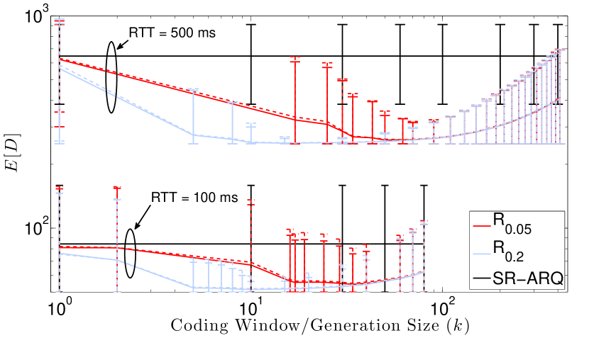
(a) $\epsilon=0.01$

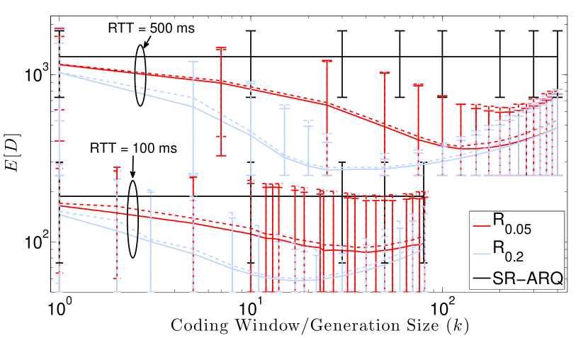
(b) $\epsilon=0.1$

Figure 4: The in-order delay for two erasure rates as a function of $k$ on a 10 Mbps link. The error bars show $2\sigma_{D}$ above and below the mean. The analytical and simulated results are represented using solid and dotted lines respectively. Note the log scale of both the x-axis and y-axis.

Results for four different networks/links are shown in Figure 4. The simulation was developed in Matlab utilizing a model similar to that presented in Section III, although several of the assumptions are relaxed. The time it takes to retransmit coded packets after feedback is received is taken into account. Furthermore, the number of generations preventing delivery is not limited to a single $BDP$ of packets, which increases the probability of head-of-line blocking. Both of these relaxations effectively increases the delay experienced by a packet. Finally, the figure shows the delay of an idealized version of SR-ARQ where we assume infinite buffer sizes and the delay is measured from the time a packet is first transmitted until the time it is delivered in-order.

Figure 4 illustrates that adding redundancy and/or choosing the correct coding window/generation size can have major implications on the in-order delay. Not only does choosing correctly reduce the delay, but can also reduce the jitter. However, it is apparent when viewing $\mathbb{E}\left[D\right]$ as a function of $k$ that the proper selection of $k$ for a given $R$ is critical for minimizing $\mathbb{E}\left[D\right]$ and $\mathbb{E}\left[D^{2}\right]$. In fact, Figure 4 indicates that adding redundancy and choosing a moderately sized generation is needed in most cases to ensure both are minimized.

Before proceeding, it is important to note that a certain level of redundancy is needed to see benefits. Each curve shows results for $R>\nicefrac{{1}}{{1-\epsilon}}$. For $R\leq\nicefrac{{1}}{{1-\epsilon}}$, it is possible to see in-order delays and jitter worse than the idealized ARQ scheme. Consider an example where a packet loss is observed near the beginning of a generation that cannot be decoded after the first transmission attempt. Since feedback is not sent/acted upon until the end of the generation, the extra time waiting for the feedback can induce larger delays than what would have occurred under a simple ARQ scheme. We can reduce this time by reacting to feedback before the end of a generation; but it is still extremely important to ensure that the choice of $k$ and $R$ will decrease the probability of a decoding failure and provide improved delay performance.

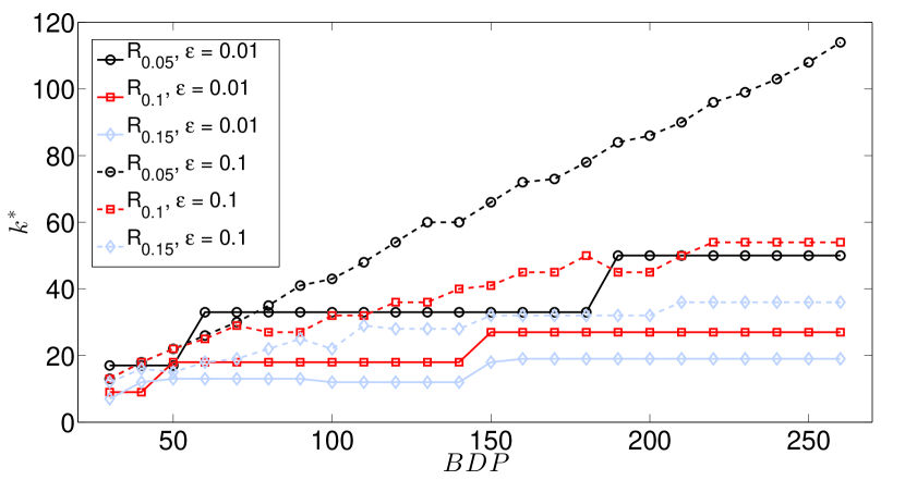
Figure 5: $k^{*}$ as a function of the $BDP$.

The shape of the curves in the figure also indicate that there are two major contributors to the in-order delay that need to be balanced. Let $k^{*}$ be the generation size where $\mathbb{E}\left[D\right]$ is minimized for a given $\epsilon$ and $R$, i.e.,

$$k^{*}=\arg\min_{k}\mathbb{E}\left[D\right].$$ (45)

To the left $k^{*}$, the delay is dominated by head-of-line blocking and resequencing delay created by previous generations. To the right of $k^{*}$, the delay is dominated by the time it takes to receive enough $dofs$ to decode the generation. While there are gains in efficiency for $k>k^{*}$, the benefits are negligible for most time-sensitive applications. As a result, we show $k^{*}$ for a given $\epsilon$ and $R$ as a function of the $BDP$ in Figure 5 and make three observations concerning this figure. First, the coding window size $k^{*}$ increases with $\epsilon$, which is opposite of what we would expect from a typical erasure code [25]. In the case of small $\epsilon$, it is better to try and quickly correct only some of the packet losses occurring within a generation using the initially transmitted coded packets while relying heavily on feedback to overcome any decoding errors. In the case of large $\epsilon$, a large generation size is better where the majority of packet losses occurring within a generation are corrected using the initially transmitted coded packets and feedback is relied upon to help overcome the rare decoding error. Second, increasing $R$ decreases $k^{*}$. This due to the receiver’s increased ability to decode a generation without having to wait for retransmissions. Third, $k^{*}$ is not very sensitive to the $BDP$ (in most cases) enabling increased flexibility during system design and implementation.

VIII-B Rate-Delay Trade-Off

While transport layer coding can help meet strict delay constraints, the decreased delay comes at the cost of throughput, or efficiency. Let $\mathbb{E}\left[D^{*}\right]$, $\sigma_{D}^{*}$, and $\eta^{*}$ be the expected in-order delay, the standard deviation, and the expected efficiency respectively that corresponds to $k^{*}$ defined in eq. (45). The rate-delay trade-off is shown by plotting $\mathbb{E}\left[D^{*}\right]$ as a function of $\eta^{*}$ in Figure 6. The expected SR-ARQ delay (i.e., the data point for $\eta=1$) is also plotted for each packet erasure rate as a reference.

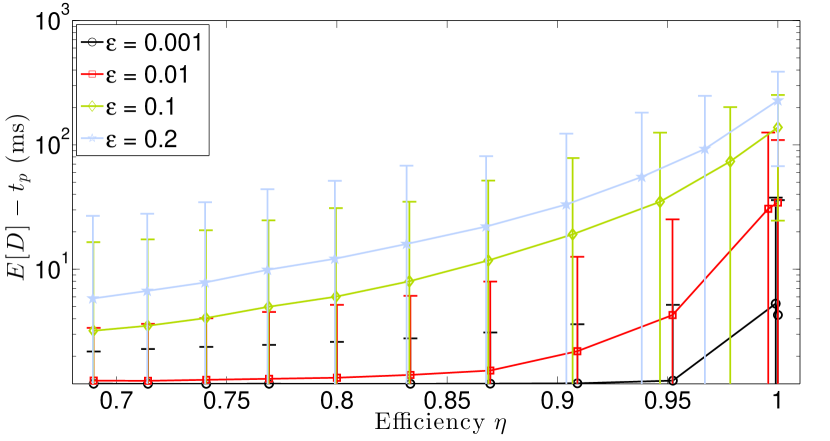
Figure 6: Rate-delay trade-off for a 10 Mbps link with a $RTT$ of 100 ms. The error bars represent $2\sigma_{D}$ above and below the mean, and the delay for ARQ is shown for $\eta=1$. Note the log scale of the y-axis.

The figure shows that an initial increase in $R$ (or a decrease in $\eta$) has the biggest effect on $\mathbb{E}\left[D\right]$. In fact, the majority of the decrease is observed at the cost of just a few percent (2-5%) of the available network capacity when $\epsilon$ is small. As $R$ is increased further, the primary benefit presents itself as a reduction in the jitter (or $\mathbb{E}\left[D^{2}\right]$). Furthermore, the figure shows that even for high packet erasure rates (e.g., $20\%$), strict delay constraints can be met as long as the user is willing to sacrifice throughput.

VIII-C Real-World Comparison

We finally compare the analysis with experimentally obtained results in Figure 7 and show that our analysis provides a reasonable approximation to real-world protocols. The experiments were conducted using Coded TCP (CTCP) over an emulated network similar to the one used in [7] with a rate of 25 Mbps and a $RTT$ of 60 ms. The only difference between our setup and theirs was that we fixed CTCP’s congestion control window size ($cwnd$) to be equal to the $BDP$ of the network in order to eliminate the affects of fluctuating $cwnd$ sizes.

There are several contributing factors for the differences between the experimental and analytical results shown in the figure. First, the analytical model approximates the algorithm used in CTCP. Where we assume feedback is only acted upon at the end of a generation, CTCP proactively acts upon feedback and does not wait until the end of a generation to determine if retransmissions are required. CTCP’s standard deviation is less than the analytical standard deviation as a result. Second, the experiments include additional processing time needed to accomplish tasks such as coding and decoding, while the analysis does not. Finally, the assumptions made in Sections III and V effectively lower bounds $\mathbb{E}\left[D\right]$ and $\mathbb{E}\left[D^{2}\right]$. Regardless, the analysis does provide a fairly good estimate of the in-order delay and can be used to help inform decisions regarding the appropriate generation size to use for a given network/link.

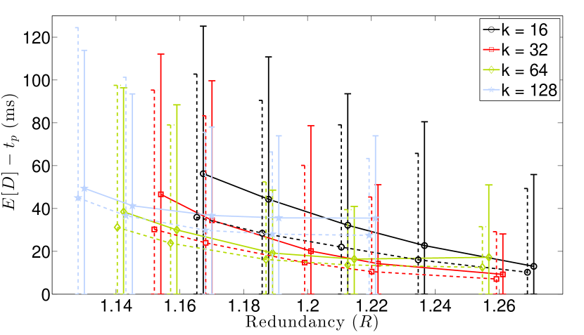
Figure 7: Experimental (solid lines) and analytical (dotted lines) results for various $k$ over a 25 Mbps link with $RTT=60\text{ ms}$ and $\epsilon=0.1$.

IX Conclusion

In this paper, we addressed the use of transport layer coding to improve application layer performance. A coding algorithm and an analysis of the in-order delivery delay’s first two moments were presented, in addition to numerical results addressing when and how much redundancy should be added to a packet stream to meet a user’s delay constraints. These results showed that the coding window size that minimizes the expected in-order delay is largely insensitive to the $BDP$ of the network for some cases. Finally, we compared our analysis with the measured delay of an implemented transport protocol, CTCP. While our analysis and the behavior of CTCP do not provide a one-to-one comparison, we illustrated how our work can be used to help inform system decisions when attempting to minimize delay.

References

- [1] Sandvine, “Global Internet Phenomena.” Online, May 2014.
- [2] Y. Xia and D. Tse, “Analysis on Packet Resequencing for Reliable Network Protocols,” in INFOCOM, vol. 2, pp. 990–1000, Mar. 2003.
- [3] J. K. Sundararajan, D. Shah, M. Médard, S. Jakubczak, M. Mitzenmacher, and J. Barros, “Network Coding Meets TCP: Theory and Implementation,” Proc. of the IEEE, vol. 99, pp. 490–512, Mar. 2011.
- [4] V. Subramanian, S. Kalyanaraman, and K. K. Ramakrishnan, “Hybrid Packet FEC and Retransmission-Based Erasure Recovery Mechanisms for Lossy Networks: Analysis and Design,” in COMSWARE, 2007.
- [5] O. Tickoo, V. Subraman, S. Kalyanaraman, and K. K. Ramakrishnan, “LT-TCP: End-to-End Framework to Improve TCP Performance Over Networks with Lossy Channels,” in IWQoS, pp. 81–93, 2005.
- [6] B. Ganguly, B. Holzbauer, K. Kar, and K. Battle, “Loss-Tolerant TCP (LT-TCP): Implementation and Experimental Evaluation,” in MILCOM, 2012.
- [7] M. Kim, J. Cloud, A. ParandehGheibi, L. Urbina, K. Fouli, D. J. Leith, and M. Médard, “Congestion Control for Coded Transport Layers,” in ICC, June 2014.
- [8] T. Ho, M. Médard, R. Koetter, D. Karger, M. Effros, J. Shi, and B. Leong, “A Random Linear Network Coding Approach to Multicast,” IEEE Trans. on Info. Theory, vol. 52, no. 10, pp. 4413–4430, 2006.
- [9] A. Heidarzadeh, Design and Analysis of Random Linear Network Coding Schemes: Dense Codes, Chunked Codes and Overlapped Chunked Codes. Ph.D. Thesis, Carleton University, Ottawa, Canada, Dec. 2012.
- [10] D. Lucani, M. Médard, and M. Stojanovic, “Broadcasting in Time-Division Duplexing: A Random Linear Network Coding Approach,” in NetCod, pp. 62–67, June 2009.
- [11] D. Lucani, M. Médard, and M. Stojanovic, “Online Network Coding for Time-Division Duplexing,” in GLOBECOM, Dec. 2010.
- [12] D. Lucani, M. Stojanovic, and M. Médard, “Random Linear Network Coding For Time Division Duplexing: When To Stop Talking And Start Listening,” in INFOCOM, pp. 1800–1808, Apr. 2009.
- [13] T. Dikaliotis, A. Dimakis, T. Ho, and M. Effros, “On the Delay of Network Coding Over Line Networks,” in ISIT, June 2009.
- [14] M. Nistor, R. Costa, T. Vinhoza, and J. Barros, “Non-Asymptotic Analysis of Network Coding Delay,” in NetCod, June 2010.
- [15] E. Drinea, C. Fragouli, and L. Keller, “Delay with Network Coding and Feedback,” in ISIT, pp. 844–848, June 2009.
- [16] A. Eryilmaz, A. Ozdaglar, and M. Médard, “On Delay Performance Gains From Network Coding,” in CISS, pp. 864–870, Mar. 2006.
- [17] B. Swapna, A. Eryilmaz, and N. Shroff, “Throughput-Delay Analysis of Random Linear Network Coding for Wireless Broadcasting,” IEEE Trans. on Information Theory, vol. 59, pp. 6328–6341, Oct. 2013.
- [18] H. Yao, Y. Kochman, and G. W. Wornell, “A Multi-Burst Transmission Strategy for Streaming Over Blockage Channels with Long Feedback Delay,” IEEE JSAC, vol. 29, pp. 2033–2043, Dec. 2011.
- [19] M. Nistor, J. Barros, F. Vieira, T. Vinhoza, and J. Widmer, “Network Coding Delay: A Brute-Force Analysis,” in ITA, Jan. 2010.
- [20] J. Sundararajan, P. Sadeghi, and M. Médard, “A Feedback-Based Adaptive Broadcast Coding Scheme for Reducing In-Order Delivery Delay,” in NetCod, June 2009.
- [21] W. Zeng, C. Ng, and M. Médard, “Joint Coding and Scheduling Optimization in Wireless Systems with Varying Delay Sensitivities,” in SECON, pp. 416–424, June 2012.
- [22] G. Joshi, Y. Kochman, and G. W. Wornell, “On Playback Delay in Streaming Communication,” in ISIT, pp. 2856–2860, July 2012.
- [23] G. Joshi, Y. Kochman, and G. Wornell, “Effect of Block-Wise Feedback on the Throughput-Delay Trade-Off in Streaming,” in INFOCOM Workshop on Contemporary Video, Apr. 2014.
- [24] M. Tömösközi, F. H. Fitzek, F. H. Fitzek, D. E. Lucani, M. V. Pedersen, and P. Seeling, “On the Delay Characteristics for Point-to-Point Links using Random Linear Network Coding with On-the-Fly Coding Capabilities,” in European Wireless 2014, May 2014.
- [25] R. Koetter and F. Kschischang, “Coding for Errors and Erasures in Random Network Coding,” IEEE Trans. on Information Theory, vol. 54, pp. 3579–3591, Aug. 2008.